Ionization cross sections for low energy electron transport

Abstract

Two models for the calculation of ionization cross sections by electron impact on atoms, the Binary-Encouter-Bethe and the Deutsch-Märk models, have been implemented; they are intended to extend and improve Geant4 simulation capabilities in the energy range below 1 keV. The physics features of the implementation of the models are described, and their differences with respect to the original formulations are discussed. Results of the verification with respect to the original theoretical sources and of extensive validation with respect to experimental data are reported. The validation process also concerns the ionization cross sections included in the Evaluated Electron Data Library used by Geant4 for low energy electron transport. Among the three cross section options, the Deutsch-Märk model is identified as the most accurate at reproducing experimental data over the energy range subject to test.

I Introduction

Various experimental research topics require the capability of simulating electron interactions with matter over a wide range - from the nano-scale to the macroscopic one: some examples are ongoing investigations on nanotechnology-based particle detectors, scintillators and gaseous detectors, radiation effects on semiconductor devices, background effects on X-ray telescopes and biological effects of radiation.

Physics tools for the simulation of electron interactions are available in all Monte Carlo codes based on condensed and mixed transport schemes [1], like EGS [2, 3], FLUKA [4, 5], Geant4 [7, 6], MCNPX [8], Penelope [9] and PHITS [10]. General-purpose Monte Carlo codes based on these transport schemes typically handle particles with energy above 1 keV; Geant4 and Penelope extend their coverage below this limit.

In the lower energy end below 1 keV, so-called “track structure” codes handle particle interactions based on discrete transport schemes; they provide simulation capabilities limited to a single target, or a small number of target materials, and are typically developed for specific application purposes. Some examples of such codes are OREC [11], PARTRAC [12], Grosswendt’s Monte Carlo for nanodosimetry [13], TRAMOS [14], and Geant4 models for microdosimetry simulation in water [15].

The developments described in this paper address the problem of endowing a general purpose, large scale Monte Carlo system for the first time with the capability of simulating electron impact ionisation down to the scale of a few tens of electronvolts for any target element. For this purpose, models of electron impact ionization cross sections suitable to extend Geant4 capabilities in the low energy range have been implemented and validated with respect to a large set of experimental measurements.

The validation process, which involves experimental data pertinent to more than 50 elements, also addresses the ionization cross sections encompassed in the Evaluated Electron Data Library (EEDL) [16], which are used in Geant4 low energy electromagnetic package [17, 18]. To the best of the authors’ knowledge, this is the first time that EEDL is subject to extensive experimental benchmarks below 1 keV.

II Overview of electron ionization in Geant4

The Geant4 toolkit provides various implementations of electron ionization based on a condensed-discrete particle transport scheme. Two of them, respectively based on EEDL [19] and on the analytical models originally developed for the Penelope [9] Monte Carlo system, are included in the low energy electromagnetic package; another implementation is available in the standard [20] electromagnetic package. In addition, a specialized ionization model for interactions with thin layers of material, the photoabsorption-ionization (PAI) model [21], is implemented in Geant4.

The EEDL data library tabulates electron ionization cross sections in the energy range between 10 eV and 100 GeV; nevertheless, due to intrinsic limitations of the accuracy of EEDL and its companion Evaluated Photon Data Libray (EPDL) [22] highlighted in the documentation of these compilations, the use of Geant4 low energy models based on them was originally recommended for incident electron energies above 250 eV [19]. This limit of applicability was an “educated guess” rather than a rigorous estimate of validity of the theoretical calculations tabulated in EEDL and EPDL. The lower energy limit of Penelope’s applicability is generically indicated by its authors as “a few hundred electronvolts” [23]. The lower limit of applicability of Geant4 standard electromagnetic package is 1 keV.

The validation of Geant4 models for electron transport based on the EEDL data library and on Penelope-like models is documented in [24] for what concerns the energy deposition in extended media.

Ionization models suitable for microdosimetry simulation, which operate in a discrete particle transport scheme, are available in Geant4 for electron interactions in water [15]; they are applicable for energies down to the electronvolt scale. The cross section models implemented in that context are specific to one material (liquid water); due to lack of pertinent experimental data, their validation is still pending.

III Software development process

The developments described in this paper adopt an iterative-incremental process consistent with the Unified Process [25]. The features and results documented in the following sections correspond to the first cycle of a wider project concerning the development and assessment of models for multi-scale electron transport [26, 27], which is motivated by multi-disciplinary experimental applications. A characterizing feature of the Unified Process, which differentiates it from other widespread software life-cycle models adopting a waterfall [28] approach, is the production of concrete deliverables even at intermediate stages of the project: this development cycle has enabled the validation and comparative evaluation of different physics models, and has produced a data library usable in multiple environment.

The software described and validated in the following sections is intended for release in the Geant4 toolkit following the publication of this paper.

III-A Physics models

The developed software tools concern the calculation and validation of cross sections for the ionization of an atom by electron impact at energies below 10 keV: they are focused on the total cross section for single ionization, namely the emission of one electron from a neutral atom, irrespective of the shell from which the electron is emitted. Collective phenomena and solid state effects are outside their scope, as well as the treatment of electron interactions with matter other than ionization.

Two ionization cross section models, which specifically address the low energy range, have been implemented: the Binary-Encounter-Bethe (BEB) model [29] and the Deutsch-Märk (DM) [30] model. Their accuracy at reproducing experimental data is extensively investigated in the following sections, along with the validation of the ionization cross sections included in EEDL, currently used by Geant4.

The theoretical models adopted in the software implementation have a wider scope of applicability: they can calculate cross sections for the ionization of individual shells as well as for multiple ionized atoms and for molecules. The assessment of these additional capabilities is intended to be the object of further cycles in the software process, to be documented in dedicated papers.

III-B Software design

The software adopts a policy-based class design [31]; this technique was first introduced in a general-purpose Monte Carlo system in [15]. This programming paradigm allows the exploitation of the developed models in different contexts with great versatility, without imposing the burden of inheritance from a pre-defined interface, since policies are syntax-oriented, rather than signature-oriented.

Preliminary evaluations [33, 32] indicate that policy-based design contributes to achieve better computational performance than conventional inheritance in the calculation of cross sections, thanks to compile-time binding. This feature is relevant to the computationally intensive domain of Monte Carlo particle transport, especially at low energies, where discrete transport methods, involving a large number of steps and accounting for individual collisions with the interacting medium, may be required for precise calculation.

The classes responsible for the calculation of ionization cross sections conform to the cross section policy defined in [33, 32]. The policy consists of a CrossSection function, whose arguments are associated with characteristics of the incident particle and the target atom; it returns the value of the cross section calculated in the conditions specified by the arguments.

III-C Implementation

The Binary-Encounter-Bethe and Deutsch-Märk models are implemented according to the analytical formulations devised by their original authors. The implementation is based on the latest revisions of the models available in the literature.

Both cross section calculations involve a few atomic parameters; the Deutsch-Märk model also involves some empirical parameters derived from fits to experimental data. The software implementation is based on the parameters documented in the literature by the original authors of the theoretical models; alternative sources were used in the software implementation, when the original sources are not publicly accessible, or not specified. The differences of the implementation with respect to the original models and their implications are discussed in detail in the following sections.

III-D Software Verification and Validation

The verification process ascertained whether the cross sections calculated by the software implementation of the BEB and DM models are consistent with the original values published by the respective authors. The validation process involves comparisons with experimental data to ascertain whether the two new models and the EEDL data library describe electron ionization cross sections accurately.

The software verification and validation follow the guidelines of the pertinent IEEE Standard [34]. Nevertheless, these two processes are intertwined: the verification of compatibility with original calculations cannot be completly disjoint from the assessment whether any detected discrepancies would affect the model accuracy significantly with respect to experimental data.

Some of the reference cross section values for the verification and validation process, which are not available in numerical format, were digitized from published plots by means of the Engauge [35] software. The uncertainty associated with the digitization process was evaluated by digitizing plots whose entries were known a priori; it is smaller than 1%.

IV The Binary-Encounter-Bethe model

IV-A Theoretical background

The Binary-Encounter-Bethe model is a simplified version of the Binary-Encounter-Dipole (BED) model [29] proposed by Kim and Rudd to calculate electron impact ionisation cross sections.

The BED model combines a modified form of the Mott cross section [36] with the Bethe theory [37]. Mott theory describes the collision of two free electrons: it is expected to give good results for small impact parameters, or hard collisions, but it must be corrected for large impact parameters, or soft collision, where dipole interaction is prevalent, especially at high incident electron energies. Several attempts have been made to simultaneously describe hard and soft collisions [38, 39, 40, 41], but they generally failed in finding the proper mixing between these two different physical situations.

The BED model was proposed to describe in a parameter-free fashion the impact of a free electron on a bound one: it is able to determine the proper mixing by requiring the asymptotic behaviour of the ionization cross section to coincide with the one obtained in Bethe’s theory, but some issues remain open on how to describe within the model the fact that the outgoing primary and secondary electrons are undistinguishable. This crucial feature is included only in the Mott cross section. These shortcomings can explain the observed difference between the predictions of the BED and Deutsch-Märk model, which, as discussed in the following section, is to a large extent a phenomenological description of ionization processes.

The BED model prescribes procedures to evaluate the energy distribution of the ejected electron for each subshell using the binding energy, average kinetic energy and dipole oscillator strength for each subshell. The agreement of BED with known experimental data is of the order of 10% in the region from the threshold to some keV.

The oscillator strengths required in the BED formula can be obtained by theoretical calculations or experimental photoionization cross sections; nevertheless, they are not easily available for every atom and for each subshell. Although the BED model shows qualitatively good agreement with experimental data for many atoms (e.g. H, He, Ne, Rb) [29, 42], the difficult availability of these components of its formulation limits its practical use.

The BEB model [29] was proposed as a simplification of the BED model, when the differential dipole oscillator strength is unknown. It assumes a simple form for the oscillator strengths, which approximates the shape of the oscillator strength for ionization of the ground state of hydrogen.

The BEB cross section for the ionization of subshell i is given by:

$$\sigma_{BEB,i}=\frac{S}{t+(u+1)/n}\left[\frac{\text{ln}(t)}{2}\left(1-\frac{1}{t^{2}}\right)+1-\frac{1}{t}-\frac{\text{ln}(t)}{t+1}\right]$$ (1)

where:

$$t=\frac{T}{B},~{}~{}~{}~{}~{}u=\frac{U}{B},~{}~{}~{}~{}~{}S=4\pi a^{2}_{0}N\left(\frac{R}{B}\right)^{2}$$ (2)

In the above equations T is the incident electron energy, t and u are normalized incident and kinetic energies, $n$ is the principal quantum number (only taken into account when greater than 2), a₀ is the Bohr radius and R is the Rydberg constant. The BEB model involves three atomic parameters for each subshell of the target atom, as shown in (1): the electron binding energy B, the average electron kinetic energy U and the occupation number N. The sum over all subshells i gives the total cross section; in practice, only the valence shell and a few outer subshells contribute significantly to determine the total cross section value.

In equation (1), the term associated with the first logarithmic function represents distant collisions (i. e. large impact parameters) dominated by the dipole interaction, and the rest of the terms represent close collisions described by the Mott cross section; the second logarithmic function originates from the interference of direct and exchange scattering.

IV-B Implementation of the BEB model

The BEB cross section model is implemented according to (1).

The atomic parameters originally used by the authors of the model have been documented in the literature only for a small number of target elements; therefore, to satisfy the requirement of general applicability in a large scale Monte Carlo system, alternative compilations of parameters, covering the whole periodic system, are utilized in the software implementation.

The electron binding energies (except for the valence electron) and average electron kinetic energies appearing in the original formulation of the Binary-Encounter-Bethe model derive from relativistic Dirac-Fock calculations [43]; since the original numerical values are not publicly available, they were replaced in the code implementation by the values reported in in the Evaluated Atomic Data Library (EADL) [44]. EADL was also used in the software implementation to retrieve the occupation numbers of each subshell, since the source of these parameters in the original BEB calculations is not explicitly documented in the literature.

The choice of EADL in the software implementation as an alternative source of the atomic parameters was mainly dictated by the limited availability of compilations of mean electron energies covering the whole periodic system; other parameters, such as atomic binding energies and occupation numbers, were taken from the same source for consistency.

Both in the original formulation of the model and in the software implementation the binding energy for the valence electron is obtained from the compilation of experimental ionization energies [45] included in the NIST (National Institute of Standards and Technology) Physics Reference Data.

IV-C Verification of the BEB model implementation

The correctness of the BEB model implementation was verified by comparing quantitatively cross sections calculated with the same atomic parameters (binding energies, ionization potentials and electron kinetic energies) used by the original authors with reference values published in the literature. The results of the software implementation are consistent with the original references; an example is illustrated in Fig. 1.

Figure 1: BEB cross section for electron impact on gallium calculated by the software (white squares) and original values (black squares), as a function of energy.

Nevertheless, as discussed in section IV-B, the software implementation uses different values of the the atomic parameters involved in (1), since the original ones are documented only for a small number of elements. The resulting cross section values are sensitive to this modification, as one can observe in Fig. 2; the extent of alteration with respect to the original values depends on the element.

Figure 2: Effect of atomic parameters on BEB cross section for electron impact on nitrogen: cross sections calculated by the implemented software (white squares) with parameters as in section IV-B, original values (black squares), calculations as in section IV-B except for atomic binding energies taken from Lotz’s compilation as in the DM model (asterisks) and for average electron kinetic energies as in the original formulation (white triangles), and with all atomic parameters taken from EADL (white circles).

An extensive investigation of the effect of atomic electron binding energies on various physics quantities relevant to Monte Carlo particle transport, including the cross sections calculated by the BEB model, is reported in [55]. The effect of atomic parameters on the accuracy of the BEB model at reproducing experimental data is discussed in section VIII.

V The Deutsch-Märk model

V-A Theoretical background

The Deutsch-Märk formalism was originally developed for the calculation of atomic ionization cross sections [30]; it has been subject to evolution [46, 47, 48, 49, 50] since its first formulation.

The DM model has its origin in a classical binary encounter approximation derived by Thomson [51] and its improved form by Gryzinski [52].

The current expression of the DM formula calculates the atomic cross section $\sigma_{DM}$ for single ionization as the sum over all partial ionization cross sections corresponding to the removal of a single electron from a given atomic subshell, characterized by quantum numbers $n$ and $l$ as:

$$\sigma_{DM}=\sum_{n,l}g_{nl}\pi r^{2}_{nl}\xi_{nl}b^{(q)}_{nl}(u)\left(\frac{\text{ln}(c_{nl}u)}{u}\right)$$ (3)

In this formula $r_{nl}$ is the radius of maximum radial density of the atomic subshell with quantum numbers $n$ and $l$ and $\xi_{nl}$ is the electron occupation number in that subshell; $g_{nl}$ are weighting factors, which were determined by the original authors from a fitting procedure [30, 46] using experimental cross section data. The quantity $u$ represents the reduced energy $E/E_{nl}$, where $E$ is the energy of the incident electron and$E_{nl}$ is the ionization energy of the subshell identified by $n$ and $l$ quantum numbers. In the original authors’ calculations the values of $r_{nl}$ were taken from Desclaux’s compilation [53] and ionization energies form Lotz’s compilation [54] of atomic binding energies. The $c_{nl}$ constant is close to one except for electrons in the $d$ orbital. The sum extends over all the subshells of the target atom.

The energy-dependent function has the form:

$$b^{(q)}_{nl}(u)=\frac{A_{1}-A_{2}}{1+(u/A_{3})^{p}}+A_{2}$$ (4)

where $A_{1}$, $A_{2}$, $A_{3}$ and $p$ are constants, that were determined from measured cross sections for the various values of $n$ and $l$ [49, 50]. The superscript $q$ refers to the number of electrons in the subshell identified by $n$ and $l$.

V-B Implementation of the DM model

The DM cross section model is implemented according to (3). Most of the parameters in the implementation are taken from the sources documented by the original authors.

The values of the radius of maximal radial density derive from the review by Desclaux [53] as in the original model. The parameters of the energy dependent function are those reported in an original reference [49].

Atomic electron binding energies derive from the compilation by Lotz [54], as in the original calculations, with the exception of the binding energies for the valence electron, which are taken from NIST collection of ionization energies [45] for consistency with the BEB implementation: however, Lotz’s and NIST ionization energies are equivalent with 0.05 significance [55]. Occupation numbers are also taken from NIST Physics Reference Data, while their source is not explicitly documented in the original formulation.

Weighting factors in the software implementation are taken from original publications [46] and[47] (the former limited to the 7s orbital); although more recent values have been determined by the original authors[56], they could not be utilized in the current implementation, as they are not publicly documented.

V-C Verification of the DM model implementation

The formulation of the DM model was revised in 2004; therefore, only cross section values published since then [48, 49, 57, 58] were considered as a reference in the software verification process.

Original cross section values concerning 48 atoms were retrieved from the literature and compared to the corresponding values calculated by the software for the purpose of verification. Two examples of these comparisons are illustrated in Fig. 3 and 4. As shown in Fig. 5, in more than 2/3 of the test cases the average difference between original and calculated values is smaller than 5%; nevertheless, for a few target elements (namely argon, cerium and gadolinium) it is greater than 20%. Goodness-of-fit tests comparing the distributions of original and calculated cross sections confirm the rejection of the null hypothesis of compatibility with 0.05 significance in these cases exhibiting large discrepancies.

Figure 3: DM cross section for electron impact on carbon calculated by the software (white triangles) and original values (black triangles), as a function of energy.

Figure 4: DM cross section for electron impact on gadolinium calculated by the software (white triangles) and original values (black triangles), as a function of energy.

Figure 5: Average relative difference between DM cross sections calculated by the software and original values, as a function of the atomic number Z.

The most probable source of the observed discrepancies between original and calculated values is the different set of weighting factors used in the software implementation and in recent Deutsch-Märk calculations, as discussed in section V-B. This assumption was tested by empirically adjusting the weighting factors values in the software implementation; as a result of this operation, cross section values compatible within 1% with recently published reference ones could be obtained for the elements exhibiting large discrepancies in Fig. 5. Nevertheless, for better traceability of the results of the software, the published weighting factors of [46] and[47] were retained in the implementation.

The role of these discrepancies on the capability of the DM model implementation to reproduce experimental data is discussed in section VIII.

VI The Evaluated Electron Data Library

The Evaluated Electron Data Library includes tabulations of ionization cross sections resulting from theoretical calculations.

For close collisions, the calculations use Seltzer’s modification [59] of Møller’s binary collision cross section [60], which takes into consideration the binding of atomic electrons in a given subshell. For distant collisions, they use Seltzer’s modification [59] of Weizsäcker-Williams’ method [61, 62]; this approach is similar to the BED model in that it requires knowledge of the dipole oscillator strengths of the target, but, being primarily designed for high energy incident electrons, it may lead to unrealistic results below a few hundred eV.

Calculations by Scofield [63] were used to take into account the density effect; this correction is significant for inner shell cross sections for incident electron energies above a few hundred MeV, but this effect sets in at lower energies for outer shells.

VII Validation of electron cross section models

The electron ionization cross sections calculated by the BEB and DM models, and those tabulated in EEDL are validated through comparison with experimental data.

Cross sections for the ionization of atoms based on the BEB and DM models have been previously subject to comparison with experimental measurements (e.g. [68, 69, 70, 71, 46, 49, 57, 58]); these comparisons involve a limited number of target elements and experimental data sets, and rely on qualitative visual appraisal of the compatibility between models and measurements. They concern calculations performed by the original authors, which, as discussed in the previous sections, in some cases cannot be reproduced, as not all the original parameters in the model formulation are publicly documented.

To the best of the authors’ knowledge, the accuracy of the EEDL ionization cross section calculations has not yet been quantitatively documented in the literature.

The validation process described in this paper concerns the cross sections calculated by the software implementation, which, being intended for open source release along with the publication of this paper, are reproducible. It involves a wider collection of experimental data than previously published comparisons and concerns a larger number of elements; moreover, the compatibility between the models and experimental measurements is estimated quantitatively, based on statistical analysis methods.

VII-A Experimental measurements

The validation of the three electron ionization cross section models is based on a large set of experimental data [73] -[150] collected in the literature. The experiments were performed with different techniques and measured a variety of physical observables, which are not always exhaustively documented in the related publications. Some papers do not report the uncertainties of the measurements.

The reference data include measurements of single ionization, i.e. the emission of a single electron as a result of the primary electron’s impact, as well as experiments that did not distinguish whether more than one electron had been emitted from the target atom. When multiple ionization is involved, a further possible source of ambiguity depends on whether the measurements concerned the so-called “total counting” cross section, which accounts for the number of ions produced,

$$\sigma_{\text{counting}}=\sum{\sigma^{n+}}$$ (5)

or the so-called “total gross” cross section, which is determined by measuring the total ion current,

$$\sigma_{\text{gross}}=\sum{n\sigma^{n+}}$$ (6)

where $n$ represents the number of ionizations. Multiple ionization is generally small with respect to single ionization: for instance, for several elements cross sections for double ionization amount to a few percent of those for single ionization, and cross sections for triple ionization are approximately an order of magnitude smaller than for double ionization [102]. Nevertheless, the contribution of double ionization may be significant for some elements: for instance, it represents more than 20% of single ionization for lead [102].

Some experiments measured absolute cross sections; some report relative values with respect to other references, which are either experimental or theoretical calculations. Both techniques have drawbacks: the intrinsic difficulty of making accurate absolute cross section measurements and the possibility of introducing a systematic bias in relative measurements.

Other features likely to be associated with systematic effects can be identified in contradictory measurements of single and total (counting or gross) ionization cross sections: in some cases (for instance, as reported in [102] and [108, 109]) the experimental cross section for single ionization appears larger than measurements of total gross or counting cross section, of which single ionization should be a component.

Large discrepancies are evident in some of the experimental data. Some data sets pertaining to the same target element are patently inconsistent; systematic effects are likely present in some cases, where the Wald-Wolfowitz test [151] detects sequences of positive or negative differences between experimental data sets, which are incompatible with randomness.

The wide heterogeneity of the experimental data complicates the validation process; it suggests caution in the interpretation of results of agreement, or disagreement, of the theoretical models with individual measurements, and induce to privilege a statistical analysis over a wide experimental sample as an indicator of the reliability of the theoretical models for use in particle transport.

TABLE I: Percentage of test cases in which cross section models are compatible with experimental data

		All	Single	Absolute	Single
			ionization	measurement	Absolute
$<$20 eV	No. data sets	107	75	73	44
	BEB	74$\pm$4	71$\pm$5	81$\pm$5	80$\pm$6
	DM	75$\pm$4	75$\pm$5	81$\pm$5	84$\pm$6
	EEDL	36$\pm$5	39$\pm$6	38$\pm$6	43$\pm$7
20-50 eV	No. data sets	129	90	83	49
	BEB	63$\pm$5	67$\pm$5	53$\pm$6	53$\pm$8
	DM	71$\pm$4	76$\pm$5	64$\pm$6	69$\pm$7
	EEDL	17$\pm$4	21$\pm$5	13$\pm$4	16$\pm$6
50-100 eV	No. data sets	124	91	81	50
	BEB	40$\pm$5	42$\pm$6	37$\pm$6	38$\pm$7
	DM	66$\pm$5	70$\pm$5	64$\pm$6	70$\pm$7
	EEDL	18$\pm$4	24$\pm$5	9$\pm$3	14$\pm$5
100-250 eV	No. data sets	127	93	81	51
	BEB	44$\pm$5	51$\pm$6	38$\pm$6	45$\pm$8
	DM	70$\pm$4	74$\pm$5	67$\pm$6	73$\pm$7
	EEDL	39$\pm$5	49$\pm$6	28$\pm$5	41$\pm$7
250 eV-1 keV	No. data sets	79	58	43	26
	BEB	62$\pm$5	76$\pm$5	58$\pm$6	81$\pm$6
	DM	78$\pm$4	86$\pm$4	72$\pm$5	85$\pm$5
	EEDL	67$\pm$5	79$\pm$5	65$\pm$6	88$\pm$5
$>$1 keV	No. data sets	25	22	12	11
	BEB	56$\pm$5	64$\pm$6	75$\pm$5	82$\pm$6
	DM	88$\pm$3	91$\pm$3	92$\pm$3	91$\pm$4
	EEDL	72$\pm$4	73$\pm$5	100$-$12	100$-$15

VII-B Analysis method

The analysis is articulated over two stages: the first one estimates the compatibility between cross section models and experimental data; the second one evaluates whether the three models exhibit any significant differences in their compatibility with experiment.

Cross sections are compared by means of statistical methods: goodness-of-fit testing to evaluate the compatibility of the simulation models with experimental measurements for each element, and categorical analysis based on contingency tables to evaluate the overall differences in compatibility with experiment across the models.

The null hypothesis in the goodness-of-fit tests is defined as the equivalence of the simulated and experimental data distributions subject to comparison. Unless differently specified, the significance level of the tests, defined as p-value determining the region of rejection of the null hypothesis, is 0.05.

Goodness of fit tests are performed on pairs of cross section distributions; for this purpose theoretical BEB and DM cross sections are calculated at the same energies as the experimental data, and EEDL cross sections corresponding to these energies are obtained through interpolation from tabulated values.

Two types of goodness of fit tests, implemented in the Statistical Toolkit [152, 153], are exploited in the validation process: the $\chi^{2}$ [154] test and three tests for unbinned distributions based on the empirical distribution function. Their complementary characteristics address some peculiarities of the experimental sample, like the lack of documentation of some experimental uncertainties or their questionable estimate, and mitigate the risk of possible systematic effects in the validation results related to the mathematical formulation of a single algorithm.

Among non-parametric goodness-of-fit tests, the $\chi^{2}$ test takes into account experimental uncertainties explicitly. It is applied in this analysis whenever experimental errors are reported in the literature and the experimental sample subject to test encompasses at least five data (i.e. the $\chi^{2}$ test is considered applicable according to statistics practice). The $\chi^{2}$ test statistic is affected by the correct appraisal of the experimental errors: their unrealistic estimation may lead to incorrect conclusions regarding the rejection of the null hypothesis.

The Kolmogorov-Smirnov[155, 156], Anderson-Darling [157, 158] and Cramer-von Mises [159, 160] tests are applied to all comparisons. They are the only means of comparing distributions when experimental errors are unknown, or the sample size is too small for the $\chi^{2}$ statistic to be meaningful; they provide complementary information about the compatibility of the compared distributions in the cases where the $\chi^{2}$ test is applicable, but the experimental errors might have not been estimated realistically.

A criterion is defined to combine the results of the different tests: the null hypothesis is not rejected if either the p-value of the $\chi^{2}$ test or the p-values of at least two out of three unbinned goodness-of-fit tests are larger than the significance level. The combined criterion privileges the outcome of the $\chi^{2}$ test, which takes into account experimental uncertainties explicitly, and requires some evidence of consistency from unbinned tests to accept the hypothesis of compatibility with experiment in cases where experimental errors are unknown, or might have been underestimated.

The cross section model exhibiting the largest number of test cases where the null hypothesis is not rejected (i.e. appearing as the most accurate at reproducing experiment) is taken as a reference in the categorical analysis; the other models are compared to it by means of contingency tables, to determine whether they exhibit any statistically significant difference of compatibility with measurements.

Contingency tables are built on the basis of the results of goodness of fit tests on individual data samples, which are classified respectively as “fail” or “pass” according to whether the hypothesis of compatibility of experimental and calculated data is rejected or not according to the combined criterion.

The null hypothesis in the analysis of a contingency table consists of assuming the equivalence of the two categories of models it compares, regarding their compatibility with experiment.

Contingency tables are analyzed with Fisher’s exact test [161] and with the $\chi^{2}$ test applying Yates continuity correction [162]; the latter ensures meaningful results even with small number of entries in the table. Pearson $\chi^{2}$ test [163] is also performed on contingency tables, when their content is consistent with its applicability. The use of different tests in the analysis of contingency tables contributes to the robustness of the results, as it mitigates the risk of introducing systematic effects, which could be due to the peculiar mathematical features of a single test.

A 0.05 significance level is set to determine the rejection of the null hypothesis in the analysis of contingency tables, unless specified differently.

The statistical analysis is articulated in energy ranges relevant to the problem domain. The higher end above 1 keV is covered by all general-purpose Monte Carlo codes for particle transport; it is considered a conventional régime of calculation of electron-photon interactions with matter. The energy range between 250 eV and 1 keV is relevant to simulation applications using the Geant4 low energy electromagnetic package, regarding the validation of the current models and the comparison with other specialized cross section models not yet available in Geant4. The lower energy end, up to a few tens of eV, pertains to microdosimetry or nanodosimetry: the validation results assess how the implemented models, which specifically address this domain, would extend Geant4 simulation capabilities for applications not yet covered by the toolkit. The assessment in the intermediate range quantitatively investigates the possibility of extending the applicability of existing Geant4 models below the current nominal limit of 250 eV, or the need of new models, such as those studied in this paper, to fill the gap between the domain of microdosimetry simulation and conventional particle transport codes.

VIII Results

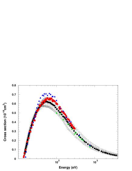
Figure 16: Cross section, Z=1: EEDL (empty circles), BEB model (empty squares), DM model (empty triangles) and experimental data from [73] (black circles), Boksenberg (reported in [72] (red squares), [74] (blue triangles) and [75] (green upside-down triangles).

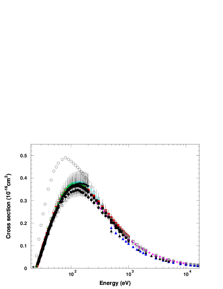
Figure 17: Cross section, Z=2: EEDL (empty circles), BEB model (empty squares), DM model (empty triangles) and experimental data from [76] (black circles), [77] (pink stars), [78] (red squares), [79] (blue triangles), [80] (green upside-down triangles), [81] (turquoise asterisks), [82] (black squares), [83] (black triangles) and [84] (black stars).

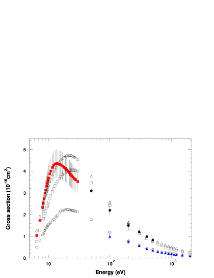
Figure 18: Cross section, Z=3: EEDL (empty circles), BEB model (empty squares), DM model (empty triangles) and experimental data from [85] (black circles), [86] (red squares) and [87] (blue triangles).

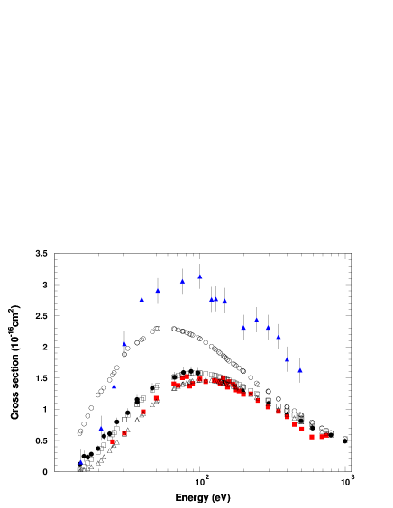
Figure 20: Cross section, Z=7: EEDL (empty circles), BEB model (empty squares), DM model (empty triangles) and experimental data from [88] (black circles), [89] (red squares) and [90] (blue triangles).

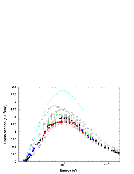
Figure 21: Cross section, Z=8: EEDL (empty circles), BEB model (empty squares), DM model (empty triangles) and experimental data from [91] (black circles), Boksenberg (reported in [72] (turquoise asterisks), [88] (blue triangles), [92] (green upside-down triangles), [75] (pink stars) and [93] (red squares).

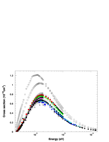
Figure 23: Cross section, Z=10: EEDL (empty circles), BEB model (empty squares), DM model (empty triangles), experimental data from [78] (black circles), [76] (black squares), [94] (black asterisks), [95] (blue triangles), [96] (red squares), [81] (green upside-down triangles), [83] (black upside-down triangles), [79] (black triangles), [97] (turquoise asterisks), [80] (pink stars) and [84] (black stars).

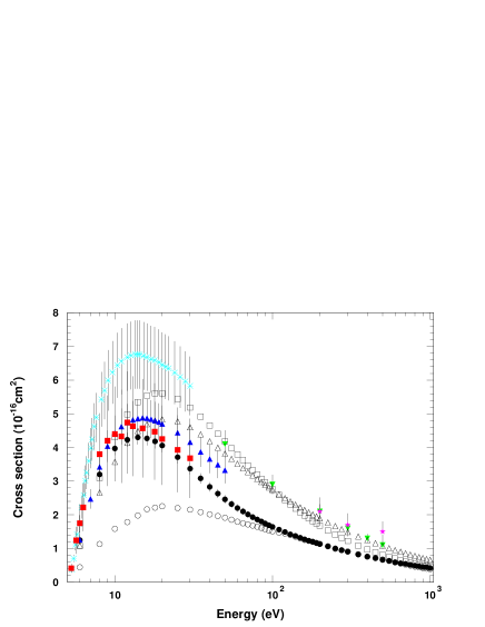
Figure 24: Cross section, Z=11: EEDL (empty circles), BEB model (empty squares), DM model (empty triangles) and experimental data from [85] (green upside-down triangles), [86] (turquoise asterisks), [98] (pink stars), [99] (black circles), [100] (blue triangles) and [101] (red squares).

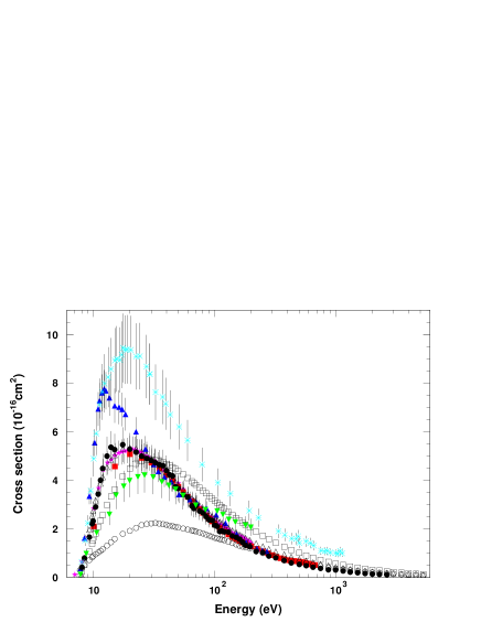
Figure 25: Cross section, Z=12: EEDL (empty circles), BEB model (empty squares), DM model (empty triangles) and experimental data from [102] (pink stars), [103] (red squares), [104] (blue triangles), [105] (black circles), [106] (green upside-down triangles) and [107] (turquoise asterisks).

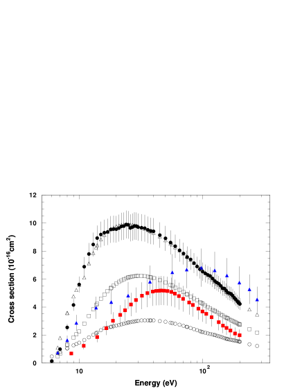
Figure 26: Cross section, Z=13: EEDL (empty circles), BEB model (empty squares), DM model (empty triangles) and experimental data from [102] (black circles), [108] (red squares) and [109] (blue triangles).

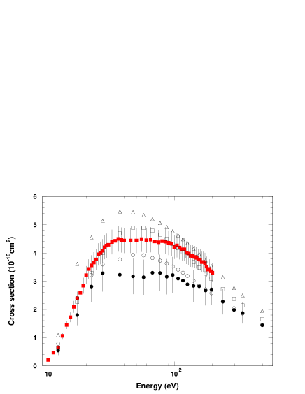
Figure 29: Cross section, Z=16: EEDL (empty circles), BEB model (empty squares), DM model (empty triangles) and experimental data from [102] (black circles) and [110] (red squares).

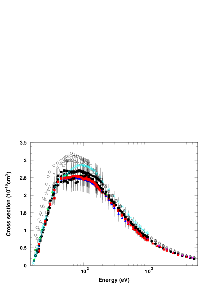
Figure 31: Cross section, Z=18: EEDL (empty circles), BEB model (empty squares), DM model (empty triangles) and experimental data from [76] (green upside-down triangles), [112] (black squares), [84] (black triangles), [81] (red squares), [113] (blue triangles), [114] (black circles), [83] (pink stars), [78] (turquoise asterisks), [115] (red triangles) and [80] (red circles).

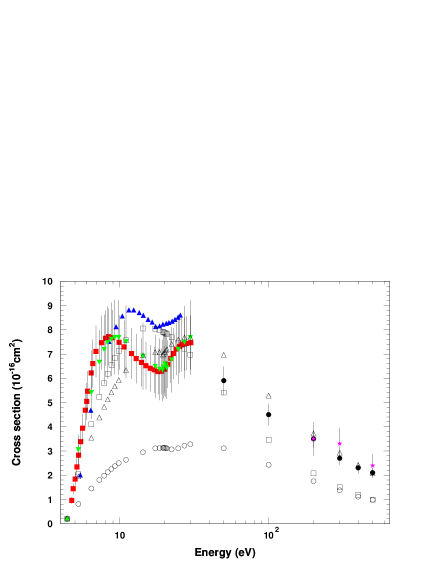
Figure 32: Cross section, Z=19: EEDL (empty circles), BEB model (empty squares), DM model (empty triangles) and experimental data from [85] (black circles), [86] (red squares), [98] (pink stars), [116] (blue triangles) and [117] (green upside-down triangles).

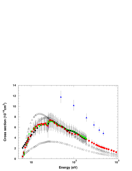
Figure 33: Cross section, Z=20: EEDL (empty circles), BEB model (empty squares), DM model (empty triangles) and experimental data from [106] (black circles), [118] (blue triangles), [119] (green upside-down triangles), [120] (red squares) and [121] (pink stars).

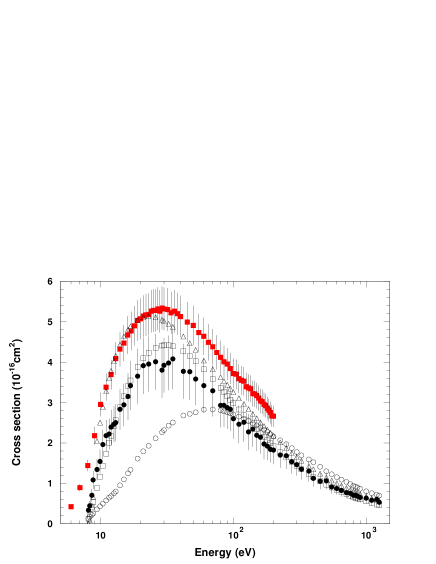
Figure 36: Cross section, Z=26: EEDL (empty circles), BEB model (empty squares), DM model (empty triangles) and experimental data from [102] (red squares) and [122] (black circles).

The cross sections calculated by the BEB, DM and EEDL models are plotted in Figs. 16-72 along with experimental data. The results of their quantitative comparisons are detailed in the next section, while possible sources of systematic effects, which might affect the validation of the simulation models, are discussed in the following sections.

VIII-A Compatibility with experimental data

The results of goodness-of-fit tests over all experimental data samples are summarized in Table I; they report the percentage of test cases in which the null hypothesis is not rejected, i.e. the theoretical models describe the data adequately. The table lists results for different experimental data types: the whole data sample, single ionization cross sections, absolute measurements, and absolute measurements of single ionization.

The results over the whole data sample are visualized in Fig. 6, where one can observe that the DM model exhibits the best overall compatibility with experimental data, while EEDL capability at reproducing measurements drops significantly below the limit of 250 eV recommended for its use in Geant4.

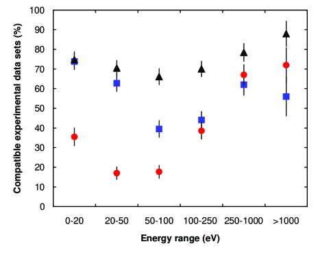
Figure 6: Fraction of test cases in which cross sections calculated by the implemented models are compatible with experimental data at 0.05 significance level: BEB model (blue squares), DM model (black triangles) and EEDL (red circles). The fraction is calculated over the whole collection of data sets.

Fig. 7 summarizes the results in relation to elements rather than individual experimental data sets; it shows the percentage of elements subject to test for which the null hypothesis is not rejected for at least one set of experimental measurements. The trend is quite similar to that observed in Fig. 6, with the DM model exhibiting in general the best capability at calculating cross sections compatible with experiment.

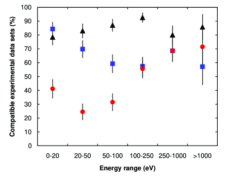
Figure 7: Fraction of elements subject to test for which cross sections calculated by the implemented models are compatible with at least one experimental data set at 0.05 significance level: BEB model (blue squares), DM model (black triangles) and EEDL (red circles).

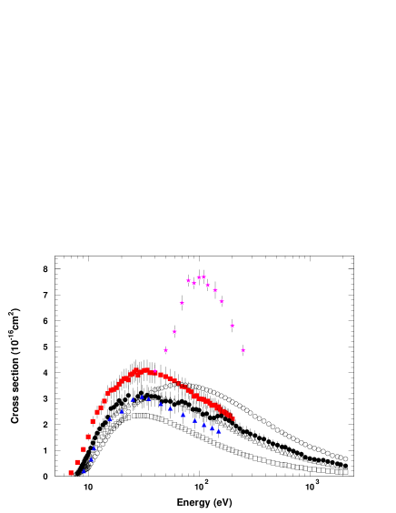
Figure 38: Cross section, Z=29: EEDL (empty circles), BEB model (empty squares), DM model (empty triangles) and experimental data from [102] (red squares), [123] (black circles), [124] (blue triangles) and [125] (pink stars).

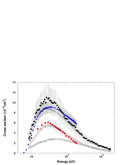
Figure 40: Cross section, Z=31: EEDL (empty circles), BEB model (empty squares), DM model (empty triangles) and experimental data from [127] (blue triangles), [128] (red squares) and [129] (black circles).

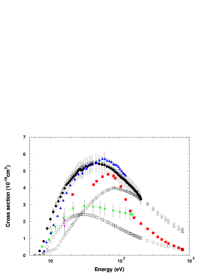
Figure 48: Cross section, Z=47: EEDL (empty circles), BEB model (empty squares), DM model (empty triangles) and experimental data from [102] (black circles), [132] (red squares), [133] (blue triangles), [134] (turquoise asterisks), [135] (pink stars) and [124] (green upside-down triangles).

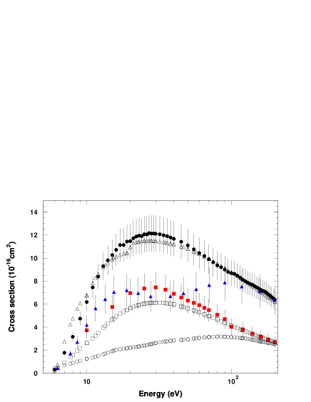
Figure 50: Cross section, Z=49: EEDL (empty circles), BEB model (empty squares), DM model (empty triangles) and experimental data from [127] (black circles), [128] (red squares) and [109] (blue triangles).

Due to the discrepancies of measurements discussed in section VII-A, the results reported in Table I and Figs. 6-7 should not be interpreted straightforwardly as estimates of the efficiency of the implemented models at calculating correct cross sections The presence of experimental data affected by systematic errors contributes to underestimate the accuracy of theoretical models, which may appear compatible with only a subset of experimental data samples: Fig. 38 and Fig. 48 are an example. On the other hand, the contradiction of patently discrepant theoretical models that appear compatible with discrepant experimental data sets contributes to overestimate the accuracy: examples are Fig. 40 and Fig. 50.

The categorical analysis estimates whether the differences of the models in compatibility with experiment are statistically significant. The results are summarized in Tables II and III, respectively comparing the compatibility of the BEB model and of EEDL over the whole collection of data samples, and in Table IV regarding the compatibility with at least one experimental sample per element.

The outcome of this statistical analysis supports the qualitative appraisal of Fig. 6 and 7. Over the whole collection of data samples, in the low energy range up to 50 eV the BEB model is equivalent to the DM one, while EEDL is statistically equivalent to the DM model above 250 eV. If one considers the compatibility with at least one experimental data set per element, the BEB model is statistically equivalent to the DM one also above 250 eV.

Some possible sources of systematic effects, which may bias the results of the validation process, are analyzed in the following sections.

TABLE II: Contingency tables related to DM and BEB cross section compatibility with experimental data

Energy	Goodness-of-fit test	All		Single		Absolute		Single
				ionization		measurement		Absolute
$<$ 20 eV		DM	BEB	DM	BEB	DM	BEB	DM	BEB
	Pass	80	79	56	53	59	59	37	35
	Fail	27	28	19	22	14	14	7	9
	p-value Fisher test	1		0.714		1		0.783
	p-value Pearson $\chi^{2}$	0.876		0.583		1		0.580
	p-value Yates $\chi^{2}$	1		0.714		1		0.782
20-50 eV		DM	BEB	DM	BEB	DM	BEB	DM	BEB
	Pass	91	81	68	60	53	44	34	26
	Fail	38	48	22	30	30	39	15	23
	p-value Fisher test	0.235		0.250		0.208		0.146
	p-value Pearson $\chi^{2}$	0.187		0.188		0.156		0.097
	p-value Yates $\chi^{2}$	0.235		0.250		0.208		0.147
50-100 eV		DM	BEB	DM	BEB	DM	BEB	DM	BEB
	Pass	82	49	64	38	52	30	35	19
	Fail	42	75	27	53	29	51	15	31
	p-value Fisher test	$<0.001$		$<0.001$		0.001		0.002
	p-value Pearson $\chi^{2}$	$<0.001$		$<0.001$		0.001		0.001
	p-value Yates $\chi^{2}$	$<0.001$		$<0.001$		0.001		0.003
100-250 eV		DM	BEB	DM	BEB	DM	BEB	DM	BEB
	Pass	89	56	69	47	54	31	37	23
	Fail	38	71	24	46	27	50	14	28
	p-value Fisher test	$<0.001$		0.001		$<0.001$		0.009
	p-value Pearson $\chi^{2}$	$<0.001$		0.001		$<0.001$		0.005
	p-value Yates $\chi^{2}$	$<0.001$		0.001		0.001		0.009
250 eV - 1 keV		DM	BEB	DM	BEB	DM	BEB	DM	BEB
	Pass	62	49	50	44	31	25	22	21
	Fail	17	30	8	14	12	18	4	5
	p-value Fisher test	0.036		0.236		0.258		1
	p-value Pearson $\chi^{2}$	0.024		0.155		0.175		not applicable
	p-value Yates $\chi^{2}$	0.037		0.236		0.258		1
$>$ 1 keV		DM	BEB	DM	BEB	DM	BEB	DM	BEB
	Pass	22	14	20	14	11	9	10	9
	Fail	3	11	2	8	1	3	1	2
	p-value Fisher test	0.025		0.069		0.590		1
	p-value Yates $\chi^{2}$	0.027		0.072		0.584		1

TABLE III: Contingency tables related to DM and EEDL cross section compatibility with experimental data

Energy	Goodness-of-fit test	All		Single		Absolute		Single
				ionization		measurement		Absolute
$<$ 20 eV		DM	EEDL	DM	EEDL	DM	EEDL	DM	EEDL
	Pass	80	38	56	29	59	28	37	19
	Fail	27	69	19	46	14	45	7	25
	p-value Fisher test	$<0.001$		$<0.001$		$<0.001$		$<0.001$
	p-value Pearson $\chi^{2}$	$<0.001$		$<0.001$		$<0.001$		$<0.001$
	p-value Yates $\chi^{2}$	$<0.001$		$<0.001$		$<0.001$		$<0.001$
20-50 eV		DM	EEDL	DM	EEDL	DM	EEDL	DM	EEDL
	Pass	91	22	68	19	53	11	34	8
	Fail	38	107	22	71	30	72	15	41
	p-value Fisher test	$<0.001$		$<0.001$		$<0.001$		$<0.001$
	p-value Pearson $\chi^{2}$	$<0.001$		$<0.001$		$<0.001$		$<0.001$
	p-value Yates $\chi^{2}$	$<0.001$		$<0.001$		$<0.001$		$<0.001$
50-100 eV		DM	EEDL	DM	EEDL	DM	EEDL	DM	EEDL
	Pass	82	22	64	22	52	7	35	7
	Fail	42	102	27	69	29	74	15	43
	p-value Fisher test	$<0.001$		$<0.001$		$<0.001$		$<0.001$
	p-value Pearson $\chi^{2}$	$<0.001$		$<0.001$		$<0.001$		$<0.001$
	p-value Yates $\chi^{2}$	$<0.001$		$<0.001$		$<0.001$		$<0.001$
100-250 eV		DM	EEDL	DM	EEDL	DM	EEDL	DM	EEDL
	Pass	89	49	69	46	54	23	37	21
	Fail	38	78	24	47	27	58	14	30
	p-value Fisher test	$<0.001$		0.001		$<0.001$		0.003
	p-value Pearson $\chi^{2}$	$<0.001$		0.001		$<0.001$		0.001
	p-value Yates $\chi^{2}$	$<0.001$		0.001		$<0.001$		0.003
250 eV - 1 keV		DM	EEDL	DM	EEDL	DM	EEDL	DM	EEDL
	Pass	62	53	50	46	31	28	22	23
	Fail	17	26	8	12	12	15	4	3
	p-value Fisher test	0.152		0.462		0.643		1
	p-value Pearson $\chi^{2}$	0.108		0.326		0.486		not applicable
	p-value Yates $\chi^{2}$	0.153		0.461		0.642		1
$>$ 1 keV		DM	EEDL	DM	EEDL	DM	EEDL	DM	EEDL
	Pass	22	18	20	16	11	12	10	11
	Fail	3	7	2	6	1	0	1	0
	p-value Fisher test	0.289		0.240		1		1
	p-value Yates $\chi^{2}$	0.289		0.241		1		1

TABLE IV: Contingency tables related to cross section compatibility with at least one experimental data set per element

Energy	Goodness-of-fit test	Models		Models
$<$ 20 eV		DM	BEB	DM	EEDL
	Pass	40	43	40	21
	Fail	11	8	11	30
	p-value Fisher test	0.612		$<0.001$
	p-value Pearson $\chi^{2}$	0.445		$<0.001$
	p-value Yates $\chi^{2}$	0.611		$<0.001$
20-50 eV		DM	BEB	DM	EEDL
	Pass	44	37	44	13
	Fail	9	16	9	40
	p-value Fisher test	0.162		$<0.001$
	p-value Pearson $\chi^{2}$	0.109		$<0.001$
	p-value Yates $\chi^{2}$	0.170		$<0.001$
50-100 eV		DM	BEB	DM	EEDL
	Pass	47	32	47	17
	Fail	7	22	7	37
	p-value Fisher test	0.001		$<0.001$
	p-value Pearson $\chi^{2}$	0.001		$<0.001$
	p-value Yates $\chi^{2}$	0.002		$<0.001$
100-250 eV		DM	BEB	DM	EEDL
	Pass	50	31	50	30
	Fail	4	23	4	24
	p-value Fisher test	$<0.001$		$<0.001$
	p-value Yates $\chi^{2}$	$<0.001$		$<0.001$
250 eV - 1 keV		DM	BEB	DM	EEDL
	Pass	28	24	28	24
	Fail	7	11	7	11
	p-value Fisher test	0.413		0.413
	p-value Pearson $\chi^{2}$	0.274		0.274
	p-value Yates $\chi^{2}$	0.412		0.412
$>$ 1 keV		DM	BEB	DM	EEDL
	Pass	12	8	12	10
	Fail	2	6	2	4
	p-value Fisher test	0.209		0.648
	p-value Yates $\chi^{2}$	0.209		0.645

VIII-B Data used in the determination of DM parameters

Some of the parameters in the formulation of the Deutsch-Märk model are determined from a fit to experimental data. The reuse of experimental data to which model parameters were fit should be taken into account in the calculation of the number of degrees of freedom in the goodness-of-fit tests concerning those experimental data sets. Nevertheless, the calculation of proper degrees of freedom is hindered by the difficulty of ascertaining which experimental data were used for the determination of the weighting factors used in the DM model implementation, and what was actually fit.

In the earliest version of the model the fit was based on a few experimental data sets for rare gases and uranium identified in [46], that were considered reliable by the original authors of the DM model. A later revision [164], which reports a subset of the weighting factors implemented in the software, mentions the inclusion of cross sections of small molecules in the determination of the new model parameters: this suggests a global fit for the determination of the weighting factors in (3) involving a set of molecules and atoms, which would have scarce relation with the issue of the degrees of freedom in goodness-of-fit tests concerning a single atom and a single experimental data sample.

According to goodness-of-fit tests, some of the cross sections calculated by the software are incompatible with 0.01 significance with experimental data exploited in the original fit of [46]: this finding hints that they retain weak memory of having been involved in a fit for the determination of model parameters. A categorical analysis comparing the compliance with experimental data used in the original authors’ fits and with data samples excluding them produces statistically equivalent results. These observations suggest that the goodness-of-fit analysis for the validation of the DM model applied in this paper is not significantly affected by the inclusion of a small subset of experimental data, which may have been somehow involved in the determination of the model parameters.

VIII-C Effect of BEB model parameters

As shown in section IV-C, the replacement of the atomic parameters used in the original formulation affects the value of the cross sections calculated by the BEB model. The effect of different values of the atomic parameters on the compatibility of the model with measurements is illustrated in Fig. 8, which compares the fraction of test cases in which BEB cross sections calculated with different atomic atomic parameters in (1) are consistent with experimental data at 0.05 significance level.

The influence of atomic parameters on the accuracy of the cross sections has been estimated through a sensitivity analysis considering the compatibility with experiment:. Cross sections were calculated with parameters as in the original model formulation, as in the software implementation, and with original average electron kinetic energies along with the other parameters as described in section IV-B. The comparisons with experimental data concerning calculations based on original parameters are necessarily limited to the elements for which original parameter values could be retrieved in the literature.

The differences in compatibility with experiment are small, and a categorical analysis based on contingency tables confirms the equivalence of the different calculations. Nevertheless, apart from the lowest energy range, the cross sections calculated with the original parameters exhibit systematically greater compatibility with experiment than those resulting from modified parameters. The difference in compatibility related to different values of the average electron kinetic energies appears small; this observation suggests that the main source of differences is related to atomic binding energies and occupation numbers. In particular, the value of the first ionization potential plays a significant role in determining the accuracy of BEB cross sections, as one can observe in Fig. 9, which compares cross sections calculated with NIST and EADL ionization potentials. An extensive evaluation of atomic binding energies and their effect in particle transport can be found in [55].

The apparent overall better performance of the model with the original parameters suggests that improved accuracy could be achieved by optimizing the source of the atomic binding energies to be used in the calculation. However, this is not a straightforward operation, since consistency should be ensured with other atomic parameters, namely occupation numbers and electron kinetic energies, involved in the formulation of the model.

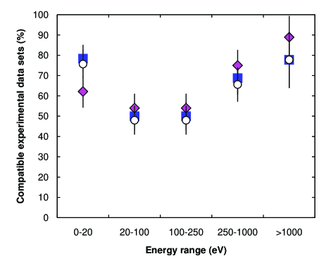
Figure 8: Fraction of test cases in which BEB cross sections calculated with different atomic atomic parameters in (1) are compatible with experimental data at 0.05 significance level: with parameters as in the software implementation described in section IV-B (blue squares), as in the original model formulation (pink diamonds) and as in section IV-B except for the average electron kinetic energies, which are as in the original model formulation (white circles). The analysis of compatibility reported in the plot is limited to the subset of elements for which the original parameters are documented in the literature.

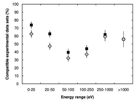
Figure 9: Fraction of test cases in which BEB cross sections calculated with NIST ionization potentials (black squares) or with EADL ones (grey diamonds) in (1) are compatible with experimental data at 0.05 significance level.

VIII-D Effect of DM model parameters

As discussed in section V-C, the cross sections calculated by the software exhibit some differences with respect to those reported in recent publications by the original authors of the model.

The observed discrepancy is not a source of concern for the accuracy of the software. In fact, when subject to the validation process described in section VII, the calculated DM cross sections are compatible with experimental data in most of the test cases exhibiting relatively large discrepancies with respect to recently published original values: apart from cerium, gadolinium and dysprosium, all the elements exhibiting greater than 10% average difference with respect to original references are compatible with experimental data with 0.05 significance over the energy range covered by measurements; the calculations for gadolinium and dysprosium are compatible with measurements above 20 eV. It is worthwhile to note that also the cross sections for cerium, gadolinium and dysprosium recently published by the original authors [58] exhibit visible differences with respect to experimental data. Regarding the discrepancy between calculated and original cross sections for argon, the controversial experimental situation depicted in Fig. 31 hinders the assessment of which calculation would produce more reliable cross sections.

The verification and validation analysis suggests that, given the quality of the available measurements, there is room for some flexibility in the determination of the DM model parameters deriving from a fit to experimental data: different parameters may modify the value of cross sections without affecting substantially the overall accuracy of the model with respect to experimental references.

It is worthwhile to note that, while a sensitivity analysis of the BEB model implementation to different values of atomic parameters appearing in its formulation, like electron binding energies, was feasible, a similar procedure would not be straightforward for the DM model, whose formulation is the result of a global fit performed by the original authors.

VIII-E Dependency on the type of cross section measurement

The theoretical models considered in this paper concern the calculation of cross sections for single ionization, while the experimental data to which they are compared include both measurements of single and “total counting” or “total gross” cross sections, that also account for multiple ionization. In principle the former should be more reliable references for the validation process, as the comparison would involve consistent physics quantities; nevertheless, this assumption could be invalidated by the heterogeneous quality of the experimental measurements discussed in section VII-A.

Some of the experimental data involved in the validation are relative cross sections with respect to reference values taken from other theoretical or experimental sources: for instance, several cross sections are reported relative to the measurements of [78], while examples of normalization with respect to theoretical calculations are the measurements of [99] (relative to Bray’s calculations [165] at 15 eV) and of [103] (relative to McGuire’s calculations [166] at 500 eV). The normalization procedure is prone to introduce further uncertainties and possible biases in the reference data.

The fraction of test cases which are compatible with experiment is shown in Figs. 10-12 for different types of experimental references: the whole sample, measurements of single ionization only, absolute cross section measurements only, and absolute measurements of single ionization. The consistency of the DM model with experiment appears independent from the type of reference data, while for BEB and EEDL cross sections one can observe some increased compatibility with measurements concerning single ionization.

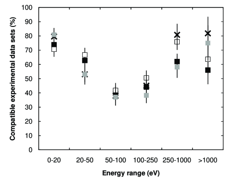
Figure 10: Fraction of test cases in which BEB cross sections are compatible with experiment at 0.05 significance level, for different types of measurements: all measurements (black squares), single ionization (white squares), absolute cross section measurements (grey squares) and absolute measurements of single ionization (crosses).

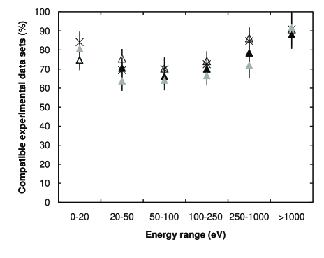
Figure 11: Fraction of test cases in which DM cross sections are compatible with experiment at 0.05 significance level, for different types of measurements: all measurements (black triangles), single ionization (white triangles), absolute cross section measurements (grey triangles) and absolute measurements of single ionization (crosses).

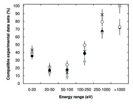
Figure 12: Fraction of test cases in which EEDL cross sections are compatible with experiment at 0.05 significance level, for different types of measurements: all measurements (black circles), single ionization (white circles), absolute cross section measurements (grey circles) and absolute measurements of single ionization (crosses).

The relative trend of compatibility with experiment of the three cross section models is scarcely affected by the nature of the reference experimental data, as one can observe in Figs. 13-15, to be compared with Fig. 6 reporting the fraction of compatible test cases for all types of measurement.

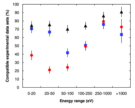
Figure 13: Fraction of test cases in which cross sections calculated by the three models are compatible with single ionization measurements at 0.05 significance level: BEB model (blue squares), DM model (black triangles) and EEDL (red circles).

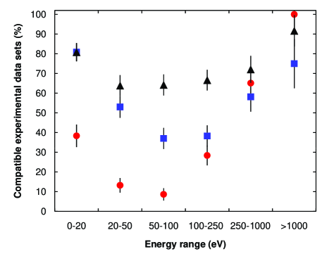
Figure 14: Fraction of test cases in which cross sections calculated by the three models are compatible with absolute ionization cross section measurements at 0.05 significance level: BEB model (blue squares), DM model (black triangles) and EEDL (red circles).

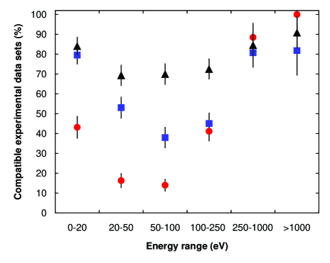
Figure 15: Fraction of test cases in which cross sections calculated by the three models are compatible with absolute measurements of single ionization cross sections at 0.05 significance level: BEB model (blue squares), DM model (black triangles) and EEDL (red circles).

The influence of the type of measurements in assessing the accuracy of a given model has been estimated through an analysis of compatibility with alternative categories of experimental references: single ionization and total counting or gross cross sections, absolute and relative measurements. The analysis, summarized in Tables V and VI, is based on contingency tables, which report the “pass” and “fail” outcome of goodness-of-fit tests associated with either category of measurements in the various energy ranges.

The DM model exhibits equivalent compatibility with single ionization measurements and total (counting or gross) experimental cross sections with 0.01 significance level over the whole energy range. The results are similar for the BEB model, with the exception of energy range between 250 eV and 1 keV, where the hypothesis of equivalent compatibility with experiment over the categories of single and total (counting or gross) cross section measurements is rejected with 0.01 significance. Regarding EEDL, equivalent behavior with respect to the two categories of experimental data is achieved at 0.01 significance level only in the low energy range below 50 eV and above 1 keV.

The BEB and DM model exhibit statistically equivalent behavior at 0.01 significance level with respect to absolute and relative measurements, with the exception of the energy range between 20 and 50 eV regarding the BEB model. No clear trend can be identified in EEDL compatibility with either type of measurements.

The compatibility of the individual models with respect to different types of experimental measurements is reflected in their comparative analysis reported in Table II: the results of comparison with respect to the DM model are consistent for all types of measurements up to 250 eV, but above 250 eV the BEB model is statistically equivalent with 0.05 significance to the DM one with respect to measurements of single ionization and absolute cross sections, while their compatibility is limited to 0.01 significance over the whole collection of data samples. The sensitivity to the type of measurements above 250 eV suggests that the equivalence of the BEB and DM models at reproducing experimental data is somewhat marginal in this energy range, therefore small variations in the experimental sample over which the two models are evaluated are prone to perturb the outcome of their comparison.

From this analysis one can conclude that the evaluation of the validity of the three models is scarcely affected by the type of experimental data taken as references: the DM model exhibits the best overall compatibility with experiment and its comparison with the other models produces consistent results at 0.01 significance level irrespective of the technique of measurement.

TABLE V: Contingency tables comparing the compatibility of theoretical models with single and total (counting or gross) cross section measurements

Energy	Goodness-of-fit test	BEB		DM		EEDL
$<$ 20 eV		Single	Total	Single	Total	Single	Total
	Pass	53	26	56	24	29	9
	Fail	22	6	19	8	46	23
	p-value Fisher test	0.339		1		0.379
	p-value Pearson $\chi^{2}$	0.254		0.971		0.297
	p-value Yates $\chi^{2}$	0.368		1		0.411
20-50 eV		Single	Total	Single	Total	Single	Total
	Pass	60	21	68	23	19	3
	Fail	30	18	22	16	71	36
	p-value Fisher test	0.173		0.091		0.076
	p-value Pearson $\chi^{2}$	0.167		0.058		not applicable
	p-value Yates $\chi^{2}$	0.236		0.092		0.108
50-100 eV		Single	Total	Single	Total	Single	Total
	Pass	38	11	64	18	22	0
	Fail	53	22	27	15	69	33
	p-value Fisher test	0.416		0.133		0.001
	p-value Pearson $\chi^{2}$	0.396		0.101		not applicable
	p-value Yates $\chi^{2}$	0.522		0.154		0.004
100-250 eV		Single	Total	Single	Total	Single	Total
	Pass	47	9	69	20	46	3
	Fail	46	25	24	14	47	31
	p-value Fisher test	0.017		0.125		$<0.001$
	p-value Pearson $\chi^{2}$	0.016		0.094		not applicable
	p-value Yates $\chi^{2}$	0.027		0.145		$<0.001$
250 eV - 1 keV		Single	Total	Single	Total	Single	Total
	Pass	44	5	50	12	46	7
	Fail	14	16	8	9	12	14
	p-value Fisher test	$<0.001$		0.011		$<0.001$
	p-value Pearson $\chi^{2}$	$<0.001$		0.005		$<0.001$
	p-value Yates $\chi^{2}$	$<0.001$		0.014		$<0.001$
$>$ 1 keV		Single	Total	Single	Total	Single	Total
	Pass	14	0	20	2	16	2
	Fail	8	3	2	1	6	1
	p-value Fisher test	0.072		0.330		1
	p-value Yates $\chi^{2}$	0.143		0.791		0.641

TABLE VI: Contingency tables comparing the compatibility of theoretical models with absolute and relative cross section measurements

Energy	Goodness-of-fit test	BEB		DM		EEDL
$<$ 20 eV		Absolute	Relative	Absolute	Relative	Absolute	Relative
	Pass	59	20	59	21	28	10
	Fail	14	14	14	13	45	24
	p-value Fisher test	0.020		0.054		0.395
	p-value Pearson $\chi^{2}$	0.016		0.035		0.368
	p-value Yates $\chi^{2}$	0.030		0.061		0.494
20-50 eV		Absolute	Relative	Absolute	Relative	Absolute	Relative
	Pass	44	37	53	38	11	11
	Fail	39	9	30	8	72	35
	p-value Fisher test	0.002		0.028		0.146
	p-value Pearson $\chi^{2}$	0.002		0.025		0.123
	p-value Yates $\chi^{2}$	0.004		0.042		0.194
50-100 eV		Absolute	Relative	Absolute	Relative	Absolute	Relative
	Pass	30	19	52	30	7	15
	Fail	51	24	29	13	74	28
	p-value Fisher test	0.448		0.557		$<0.001$
	p-value Pearson $\chi^{2}$	0.438		0.533		$<0.001$
	p-value Yates $\chi^{2}$	0.561		0.671		0.001
100-250 eV		Absolute	Relative	Absolute	Relative	Absolute	Relative
	Pass	31	25	54	35	23	26
	Fail	50	21	27	11	58	20
	p-value Fisher test	0.095		0.316		0.002
	p-value Pearson $\chi^{2}$	0.079		0.265		0.002
	p-value Yates $\chi^{2}$	0.117		0.361		0.003
250 eV - 1 keV		Absolute	Relative	Absolute	Relative	Absolute	Relative
	Pass	20	19	22	22	23	20
	Fail	12	12	10	9	9	11
	p-value Fisher test	1		1		0.595
	p-value Pearson $\chi^{2}$	0.921		0.848		0.530
	p-value Yates $\chi^{2}$	0.872		0.934		0.721
$>$ 1 keV		Absolute	Relative	Absolute	Relative	Absolute	Relative
	Pass	9	5	11	11	12	6
	Fail	3	8	1	2	0	7
	p-value Fisher test	0.111		1		0.005
	p-value Yates $\chi^{2}$	0.151		0.941		0.011

VIII-F Excitation-autoionization

Apart from direct ionization, which accounts for the ejection of a bound electron directly into the continuum, additional indirect channels of ionization may be important for open-shell atoms, such as the excitation of an inner-shell electron to an upper bound state that leads to autoionization [69]. Their contribution is generally included in the experimental measurements of total cross section for single ionization, which do not distinguish direct and indirect channels.

Contributions of indirect channels are not taken into account by the BEB model, which describes only cross sections for direct ionization, while their non explicit treatment could be partly mitigated by the semi-empirical nature of the Deutsch-Märk model. The results of the validation process in some way reflect this different approach of the BEB and DM model towards the physics phenomena that contribute to experimentally measured ionization cross sections.

The neglected contribution of excitation-autoionization could be also a reason for the rather poor compatibility of EEDL with experiment below 250 eV; nevertheless, no firm conclusion can be drawn in this respect due to the scarce documentation of how EEDL tabulations have been calculated.

Methods to calculate cross sections for excitation-autoionization are documented in the literature [69] and would be considered in future development cycles to include this process among the interactions treated by Geant4.

IX Electron cross section data library

The minimalist character of the software design and its minimal dependencies on other parts of Geant4 facilitate the exploitation of the developments described in this paper.

The developed cross section classes can be used in association with the Geant4 toolkit for the simulation of electron ionization as a discrete process, through the mechanism of a policy host class as described in [15, 33, 32]. The BEB and DM cross section code can also be exploited for the creation of data libraries to be used in the current Geant4 scheme, thus extending Geant4 simulation capabilities below the current 250 eV limit recommended for the use of the EEDL library.

A data library consisting of tabulations of ionization cross section calculated by the BEB and DM models has been produced exploiting the software developments described in this paper; the cross sections are tabulated at the same energies as in the EEDL data library. This data library can be used at the place of the current EEDL data in connection with existing implementations of Geant4 ionization process, thus giving access to the extended energy coverage and the improved accuracy of the new models in a transparent way. Its possible use is not limited to Geant4; given its wider interest, it is intended to be publicly distributed independently from Geant4 through the Radiation Safety Information Computational Center (RSICC) following the publication of this paper.

X Conclusion

Two models for the calculation of the cross sections for the ionization of atoms by electron impact, specialized in the low energy range, have been implemented: the Binary-Encounter-Bethe model and the Deutsch-Märk model. These models are intended to extend and improve the current capabilities of Geant4 for precision simulation of electron interactions.

The cross sections calculated by these models, as well as those included in the Evaluated Electron Data Library, have been subject to extensive validation in the energy range from a few eV to 10 keV.

Among the cross section models analyzed in this paper, the validation analysis has identified the Deutsch-Märk model as the most accurate for modeling electron ionization over the whole energy range considered in the test. The EEDL cross sections exhibit statistically equivalent accuracy in the energy range above 250 eV, in which they were originally recommended for use in Geant4; they are not adequately accurate to extend their usage below this threshold. In the lower energy end the Binary Encounter Bethe models exhibits statistically equivalent accuracy with respect to the Deutsch-Märk one; nevertheless, its performance appears to degrade at higher energies, presumably because it does not account for other channels than direct ionization.

Possible sources of systematic effects, which could affect the accuracy of the implementation of the theoretical models or the outcome of the validation process, have been analyzed. The values of atomic parameters, namely atomic binding energies, play a significant role in determining the accuracy of the calculated cross sections.

A cross section data library has been developed, containing tabulations of ionization cross sections calculated by the software described in this paper; it is meant for public release following the publication of this paper. The availability of cross section tabulations in a publicly distributed data library would extend the possibility of using them in other simulation systems than Geant4.

The models investigated in this paper provide more extended capabilities, that have not been exploited yet in the first development cycle described in this paper: they can describe the ionization of molecules, which could be of interest for the simulation of gaseous detectors and plasma interactions, and can calculate cross section for the ionization of inner shells, thus enabling the simulation of atomic relaxation determined by a vacancy in the shell occupation. Such extensions and improvements, as well as the development of complementary models for final state generation, are intended to be the object of further developments.

The described developments for the first time endow a general-purpose Monte Carlo simulation system of the capability of modeling electron ionization down to the energy scale relevant to nanodosimetry, for target elements spanning the whole periodic system. Nevertheless, it is worthwhile to recall that other phenomena, apart from direct ionization of atoms, should be taken into account for realistic simulation of particle interactions at very low energies: further effort should be invested for Geant4 to achieve full functionality for particle transport at nano-scale.

Due to the already significant length of this paper and its focus on cross section modeling and validation, applications of the models to real-life experimental topics are meant to be covered in dedicated papers.

Figure 19: Cross section, Z=6: EEDL (empty circles), BEB model (empty squares), DM model (empty triangles) and experimental data from [88] (black circles).

Figure 22: Cross section, Z=9: EEDL (empty circles), BEB model (empty squares), DM model (empty squares) and experimental data from [111] (black circles).

Figure 27: Cross section, Z=14: EEDL (empty circles), BEB model (empty squares), DM model (empty triangles) and experimental data from [102] (black circles).

Figure 28: Cross section, Z=15: EEDL (empty circles), BEB model (empty squares), DM model (empty triangles) and experimental data from [102] (black circles).

Figure 30: Cross section, Z=17: EEDL (empty circles), BEB model (empty squares), DM model (empty triangles) and experimental data from [111] (black circles).

Figure 34: Cross section, Z=22: EEDL (empty circles), BEB model (empty squares), DM model (empty triangles) and experimental data from Koparnski reported in [46] (black circles).

Figure 35: Cross section, Z=23: EEDL (empty circles), BEB model (empty squares), DM model (empty triangles) and experimental data from Koparnski reported in [46] (black circles).

Figure 37: Cross section, Z=28: EEDL (empty circles), BEB model (empty squares), DM model (empty triangles) and experimental data from Koparnski reported in [46] (black circles).

Figure 39: Cross section, Z=30: EEDL (empty circles), BEB model (empty squares), DM model (empty triangles) and experimental data from [126] (black circles).

Figure 41: Cross section, Z=32: EEDL (empty circles), BEB model (empty squares), DM model (empty triangles) and experimental data from [102] (black circles).

Figure 42: Cross section, Z=33: EEDL (empty circles), BEB model (empty squares), DM model (empty triangles) and experimental data from [102] (black circles).

Figure 43: Cross section, Z=34: EEDL (empty circles), BEB model (empty squares), DM model (empty triangles) and experimental data from [102] (black circles).

Figure 44: Cross section, Z=35: EEDL (empty circles), BEB model (empty squares), DM model (empty triangles) and experimental data from [111] (black circles).

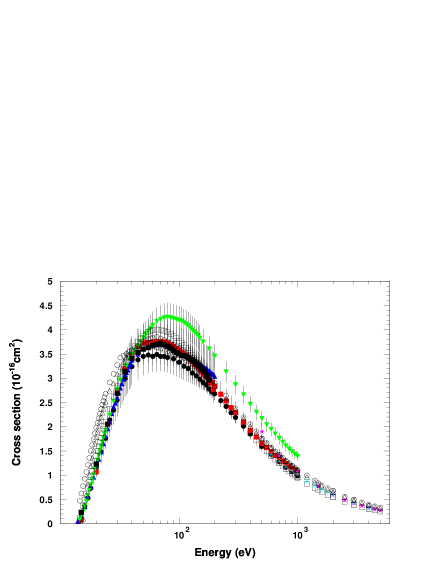
Figure 45: Cross section, Z=36: EEDL (empty circles), BEB model (empty squares), DM model (empty triangles) and experimental data from [76] (black circles), [84] (blue triangles), [81] (red squares), [83] (pink stars), [78] (green upside-down triangles), [115] (turquoise asterisks) and [80] (black squares).

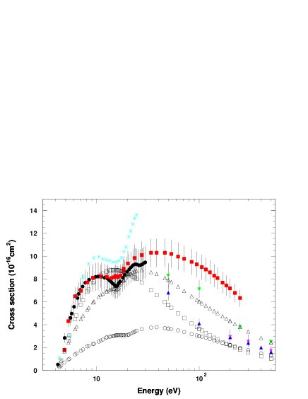
Figure 46: Cross section, Z=37: EEDL (empty circles), BEB model (empty squares), DM model (empty triangles) and experimental data from [85] (blue triangles), [86] (black circles), [98] (pink stars), [116] (turquoise asterisks), [130] (red squares) and [131] (green upside-down triangles).

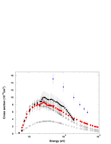
Figure 47: Cross section, Z=38: EEDL (empty circles), BEB model (empty squares), DM model (empty triangles) and experimental data from [118] (blue triangles), [106] (black circles) and [120] (red squares).

Figure 49: Cross section, Z=48: EEDL (empty circles), BEB model (empty squares), DM model (empty triangles) and experimental data from [126] (black circles).

Figure 51: Cross section, Z=50: EEDL (empty circles), BEB model (empty squares), DM model (empty triangles) and experimental data from [102] (black circles).

Figure 52: Cross section, Z=51: EEDL (empty circles), BEB model (empty squares), DM model (empty triangles) and experimental data from [102] (black circles).

Figure 53: Cross section, Z=52: EEDL (empty circles), BEB model (empty squares), DM model (empty triangles) and experimental data from [102] (black circles).

Figure 54: Cross section, Z=53: EEDL (empty circles), BEB model (empty squares), DM model (empty triangles) and experimental data from [111] (black circles).

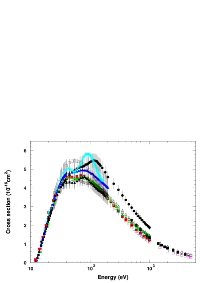
Figure 55: Cross section, Z=54: EEDL (empty circles), BEB model (empty squares), DM model (empty triangles) and experimental data from [78] (black circles), [76] (red squares), [84] (blue triangles), [81] (green upside-down triangles), [136] (turquoise asterisks), [83] (pink stars), [115] (black squares) and [137] (black triangles).

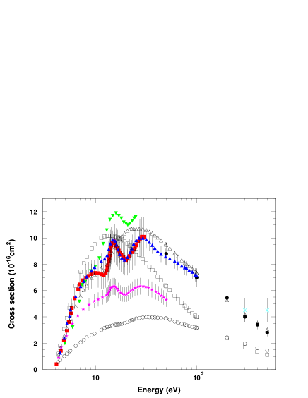
Figure 56: Cross section, Z=55: EEDL (empty circles), BEB model (empty squares), DM model (empty triangles) and experimental data from [85] (black circles), [86] (red squares), [98] (turquoise asterisks), [138] (pink stars), [116] (green upside-down triangles) and [139] (blue triangles).

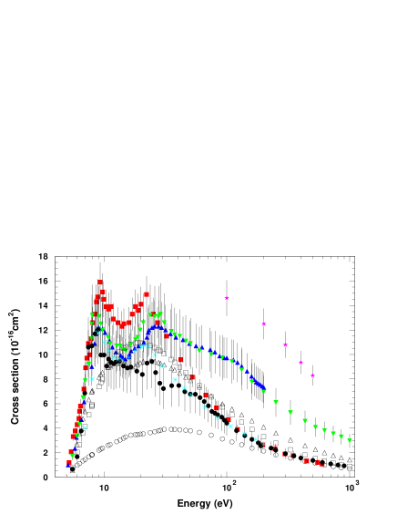
Figure 57: Cross section, Z=56: EEDL (empty circles), BEB model (empty squares), DM model (empty triangles) and experimental data from [118] (pink stars), [140] (red squares), [106] (blue triangles), [141] (black circles), [120] (green upside-down triangles), [142] (turquoise asterisks).

Figure 58: Cross section, Z=58: EEDL (empty circles), BEB model (empty squares), DM model (empty triangles) and experimental data from [143] (black circles).

Figure 59: Cross section, Z=60: EEDL (empty circles), BEB model (empty squares), DM model (empty triangles) and experimental data from [143] (black circles).

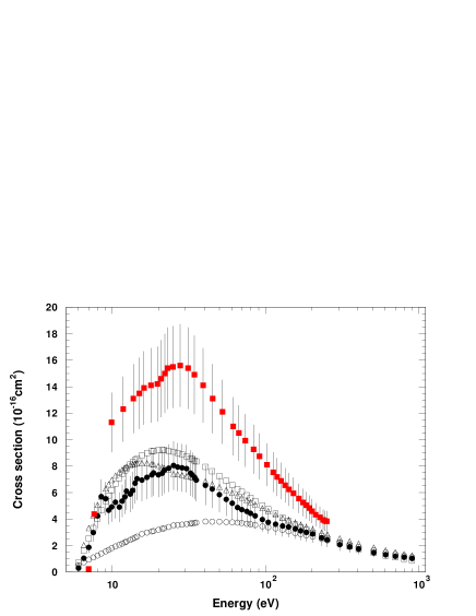
Figure 60: Cross section, Z=62: EEDL (empty circles), BEB model (empty squares), DM model (empty triangles) and experimental data from [143] (black circles) and [144] (red squares).

Figure 61: Cross section, Z=63: EEDL (empty circles), BEB model (empty squares), DM model (empty triangles) and experimental data from [141] (black circles) and [144] (red squares).

Figure 62: Cross section, Z=64: EEDL (empty circles), BEB model (empty squares), DM model (empty triangles) and experimental data from [143] (black circles).

Figure 63: Cross section, Z=66: EEDL (empty circles), BEB model (empty squares), DM model (empty triangles) and experimental data from [143] (black circles).

Figure 64: Cross section, Z=68: EEDL (empty circles), BEB model (empty squares), DM model (empty triangles) and experimental data from [143] (black circles).

Figure 65: Cross section, Z=69: EEDL (empty circles), BEB model (empty squares), DM model (empty triangles) and experimental data from [144] (black circles).

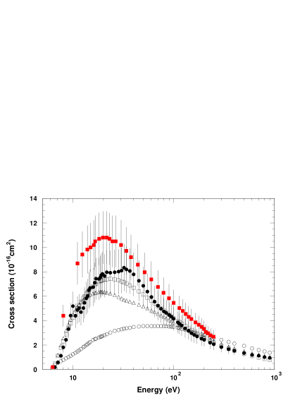
Figure 66: Cross section, Z=70: EEDL (empty circles), BEB model (empty squares), DM model (empty triangles) and experimental data from [143] (black circles) and [144] (red squares).

Figure 67: Cross section, Z=79: EEDL (empty circles), BEB model (empty squares), DM model (empty triangles) and experimental data from [125] (black circles).

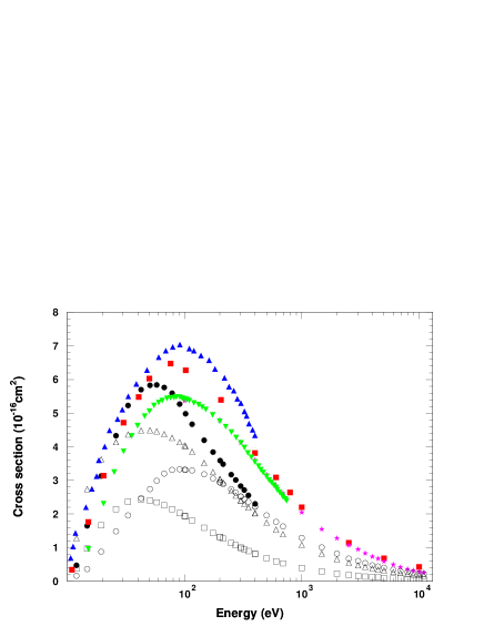
Figure 68: Cross section, Z=80: EEDL (empty circles), BEB model (empty squares), DM model (empty triangles) and experimental data from [145] (black circles), Harrison (red squares), Jones (blue triangles), Liska (pink stars) and Smith (green upside-down triangles) reported in [72].

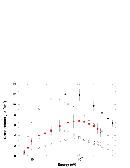
Figure 69: Cross section, Z=81: EEDL (empty circles), BEB model (empty squares), DM model (empty triangles) and experimental data from [118] (black circles) and [109] (red squares).

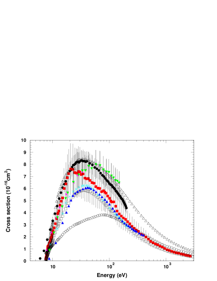
Figure 70: Cross section, Z=82: EEDL (empty circles), BEB model (empty squares), DM model (empty triangles) and experimental data from [102] (black circles), [146] (red squares), [147] (blue triangles), [148] (pink stars), [142] (turquoise asterisks) and [149] (green upside-down triangles).

Figure 71: Cross section, Z=83: EEDL (empty circles), BEB model (empty squares), DM model (empty triangles) and experimental data from [102] (black circles).

Figure 72: Cross section, Z=92: EEDL (empty circles), BEB model (empty squares), DM model (empty triangles) and experimental data from [150] (black circles).

References

- [1] M. J. Berger, “Monte Carlo calculation of the penetration and diffusion of fast charged particles”, in Methods in Computational Physics, vol. 1, Ed. B. Alder, S. Fernbach and M. Rotenberg, Academic Press, New York, pp. 135-215, 1963.
- [2] H. Hirayama, et al., “The EGS5 code system”, Report SLAC-R-730, Stanford Linear Accelerator Center, Stanford, CA, USA, 2006.
- [3] I. Kawrakow and D.W.O. Rogers, “The EGSnrc Code System: Monte Carlo Simulation of Electron and Photon Transport”, NRCC Report PIRS-701, Sep. 2006.
- [4] G. Battistoni et al., “The FLUKA code: description and benchmarking”, in AIP Conf. Proc., vol. 896, pp. 31-49, 2007.
- [5] A. Ferrari et al., “Fluka: a multi-particle transport code”, Report CERN-2005-010, INFN/TC-05/11, SLAC-R-773, Geneva, Oct. 2005.
- [6] S. Agostinelli et al., “Geant4 - a simulation toolkit” Nucl. Instrum. Meth. A, vol. 506, no. 3, pp. 250-303, 2003.
- [7] J. Allison et al., “Geant4 Developments and Applications” IEEE Trans. Nucl. Sci., vol. 53, no. 1, pp. 270-278, 2006.
- [8] J. S. Hendricks et al., “MCNPX, Version 26c”, Los Alamos National Laboratory Report LA-UR-06-7991, 2006.
- [9] J. Baro, J. Sempau, J. M. Fernández-Varea, and F. Salvat, “PENELOPE, an algorithm for Monte Carlo simulation of the penetration and energy loss of electrons and positrons in matter”, Nucl. Instrum. Meth. B, vol. 100, no. 1, pp. 31-46, 1995.
- [10] K. Niita, T. Sato, H. Iwase, H. Nose, H. Nakashima and L. Sihver, “PHITS - a particle and heavy ion transport code system”, Radiat. Meas., vol. 41, pp. 1080-1090, 2006.
- [11] R. N. Hamm, H. A. Wright, R. H. Ritchie, J. E. Turner and T. P. Turner, “Monte Carlo calculation of transport of electrons through liquid water”, in Proc. 5th Workshop on Microdosim., pp. 1037-1053, 1975.
- [12] S. Henss and H. G. Paretzke, “Biophysical modeling of radiation induced damage in chromosome”, in Proc. Biophysical modelling of radiation effects, Ed.: Adam Hilger, New York, pp. 69-76, 1992.
- [13] B. Grosswendt and S. Pszona, “The track structure of a-particles from the point of view of ionization-cluster formation in nanometric volumes of nitrogen”, Radiat. Environ. Biophys., vol. 41, no. 2, pp. 91-102, 2002.
- [14] T. Colladant, A. L’Hoir, J. E. Sauvestre and O. Flament, “Monte-Carlo simulations of ion track in silicon and influence of its spatial distribution on single event effects”, Nucl. Instrum. Meth. B, vol. 245, no. 2, pp. 464-474, 2006.
- [15] S. Chauvie et al., ”Geant4 physics processes for microdosimetry simulation: design foundation and implementation of the first set of models”, IEEE Trans. Nucl. Sci., vol. 54, no. 6, pp. 2619-2628, 2007.
- [16] S. T. Perkins et al., “Tables and Graphs of Electron-Interaction Cross Sections from 10 eV to 100 GeV Derived from the LLNL Evaluated Electron Data Library (EEDL)”, UCRL-50400 Vol. 31, 1997.
- [17] S. Chauvie, G. Depaola, V. Ivanchenko, F. Longo, P. Nieminen and M. G. Pia, “Geant4 Low Energy Electromagnetic Physics”, in Proc. Computing in High Energy and Nuclear Physics, Beijing, China, pp. 337-340, 2001.
- [18] S. Chauvie et al., “Geant4 Low Energy Electromagnetic Physics”, in 2004 IEEE Nucl. Sci. Symp. Conf. Rec., pp. 1881-1885, 2004.
- [19] J. Apostolakis, S. Giani, M. Maire, P. Nieminen, M.G. Pia, and L. Urban, “Geant4 low energy electromagnetic models for electrons and photons” INFN/AE-99/18, Frascati, 1999.
- [20] H. Burkhardt et al., “Geant4 Standard Electromagnetic Package”, in Proc. 2005 Conf. on Monte Carlo Method: Versatility Unbounded in a Dynamic Computing World, Am. Nucl. Soc., USA, 2005.
- [21] J. Apostolakis, S. Giani, L. Urban, M. Maire, A. V. Bagulya, and V. M. Grichine, “An implementation of ionisation energy loss in very thin absorbers for the GEANT4 simulation package”, Nucl. Instrum. Meth. A, vol. 453, no. 3, pp. 597-605, 2000.
- [22] D. Cullen et al., “EPDL97, the Evaluated Photon Data Library”, UCRL-50400, Vol. 6, Rev. 5, 1997.
- [23] F. Salvat, J. M. Fernandez-Varea, E. Costa, and J. Sempau, “PENELOPE - A Code System for Monte Carlo Simulation of Electron and Photon Transport”, NEA-06416, Barcelona, 2009.
- [24] A. Lechner, M.G. Pia, M. Sudhakar “Validation of Geant4 low energy electromagnetic processes against precision measurements of electron energy deposit”, IEEE Trans. Nucl. Sci., vol. 56, no. 2, pp. 398-416, 2009.
- [25] I. Jacobson, J. Booch, and J. Rumbaugh, “The Unified Software Development Process”, 1st ed., Ed: Addison-Wesley, 1999.
- [26] M. G. Pia et al., ”R&D for co-working condensed and discrete transport methods in Geant4 kernel”, in Proc. Int. Conf. on Mathematics, Computational Methods an Reactor Physics, Saratoga Springs, NY, 2009.
- [27] M. Augelli et al., ”Geant4-related R&D for new particle transport methods in 2009 IEEE Nucl. Sci. Symp. Conf. Rec., pp. 173-176, 2009.
- [28] W. W. Royce, “Managing the development of large software systems”, in Proc. IEEE WESCON, Los Angeles, pp. 328-338, 1970.
- [29] Y. K. Kim and M. E. Rudd, “Binary-encounter-dipole model for electron-impact ionization by electron impact,” Phys. Rev. A, vol. 50, pp. 3954-3967, 1994.
- [30] H. Deutsch and T. D. Märk, “Calculation of absolute electron impact ionization cross-section functions for single ionization of He, Ne, Ar, Kr, Xe, N and F,” Int. J. Mass Spectrom. Ion Processes, vol. 79, pp. R1-R8, 1987.
- [31] A. Alexandrescu, “Modern C++ Design”, Ed.: Addison-Wesley, 2001.
- [32] M. Augelli et al., ”Research in Geant4 electromagnetic physics design, and its effects on computational performance and quality assurance”, in 2009 IEEE Nucl. Sci. Symp. Conf. Rec., pp. 177-180, 2009.
- [33] M. G. Pia et al., ”Design and performance evaluations of generic programming techniques in a R&D prototype of Geant4 physics”, J. Phys.: Conf. Ser., vol. 219, pp. 042019, 2010.
- [34] IEEE Computer Society, “IEEE Standard for Software Verification and Validation”, IEEE Std 1012-2004, Jun. 2005.
- [35] M. Mitchell, Engauge Digitizer [Online]. Available: http://digitizer.sourceforge.net.
- [36] N. F. Mott, “The Collision between Two Electrons”, Proc. Royal Soc. A, vol. 126, no. 801, pp. 259-267, 1930.
- [37] H. Bethe, “Zur Theorie des Durchgangs schneller Korpuskularstrahlen durch Materie”, Ann. Phys., vol. 397, no. 3, pp. 325–400, 1930.
- [38] D. K. Jain and S. P. Khare, “Ionizing collisions of electrons with CO2, CO, H2O, CH4 and NH3”, J. Phys. B, vol. 9, no. 8, pp. 1429-1438, 1976.
- [39] S. P. Khare and W. J. Meath, “Cross sections for the direct and dissociative ionisation of NH3, H2O and H2S by electron impact ”, J. Phys. B, vol. 20, pp. 2101-2116, 1987.
- [40] S. P. Khare and A. Kumar, “Energy deposition by protons in molecular nitrogen”, Physica, vol. 100 C, no. 1, pp. 135-143, 1980.
- [41] Y. D. Kaushik, S. P. Khare and A. Kumar, “Inelastic collisions of protons with water vapour”, Physica, vol. 1006 B-C, no.1, pp. 128-134, 1981.
- [42] Y. K. Kim, J. Migdalek, W. Siegel, J. Bieron, “Electron-impact ionization cross section of rubidium,” Phys. Rev. A, vol. 57, pp. 246-254, 1998.
- [43] J. P. Desclaux, in “Methods and Techniques in Computational Chemistry: METECC”, vol. A, pp. 253-274, ed. E. Clementi, Cagliari, 1993.
- [44] S. T. Perkins et al., “Tables and Graphs of Atomic Subshell and Relaxation Data Derived from the LLNL Evaluated Atomic Data Library (EADL)”, Z=1-100, UCRL-50400 Vol. 30, 1997.
- [45] W. C. Martin, A. Musgrove, S. Kotochigova, and J. E. Sansonetti, “Ground Levels and Ionization Energies for the Neutral Atoms”, Online. Available: http://physics.nist.gov/PhysRefData/IonEnergy/ionEnergy.pdf.
- [46] D. Margreiter, H. Deutsch, and T. D. Märk, “A semiclassical approach to the calculation of electron impact ionization cross-sections of atoms: from hydrogen to uranium,” Int. J. Mass Spectrom. Ion Processes, vol. 139, pp. 127-139, 1994.
- [47] H. Deutsch, K. Becker, S. Matt, T. D. Märk, “Theoretical determination of absolute electron-impact ionization cross sections of molecules,” Int. J. Mass Spectrom., vol. 197, pp. 37-69, 2000.
- [48] H. Deutsch, P. Scheier, K. Becker, T. D. Märk, “Revised high energy behavior of the Deutsch-Märk (DM) formula for the calculation of electron impact ionization cross sections of atoms,” Int. J. Mass Spectrom., vol. 233, pp. 13-17, 2004.
- [49] H. Deutsch, P. Scheier, S. Matt-Leubner, K. Becker, T. D. Märk, “A detailed comparison of calculated and measured electron-impact ionization cross sections of atoms using the Deutsch-Märk (DM) formalism,” Int. J. Mass Spectrom., vol. 243, pp. 215-221, 2005.
- [50] H. Deutsch, P. Scheier, S. Matt-Leubner, K. Becker, T. D. Märk, “Erratum to A detailed comparison of calculated and measured electron-impact ionization cross sections of atoms using the Deutsch-Märk (DM) formalism,” Int. J. Mass Spectrom., vol. 246, p. 113, 2005.
- [51] J. J. Thomson, “Ionization by moving electrified particles”, Philos. Mag., vol. 23, no. 136, pp. 449-457, 1912.
- [52] M. Gryzinski, “Classical Theory of Atomic Collisions. I. Theory of Inelastic Collisions”, Phys. Rev., vol. 138, pp. 336-358, 1965.
- [53] J. P. Desclaux, “Relativistic Dirac-Fock expectation values for atoms with Z=1 to Z=120,” Atom. Data Nucl. Data Tables, vol. 12, pp. 311-406, 1973.
- [54] W. Lotz, “Electron binding energies in free atoms,” J. Opt. Sot. Am., vol. 60, pp. 206-210, 1970.
- [55] M. G. Pia et al., “Evaluation of atomic electron binding energies for Monte Carlo particle transport”, Submitted to IEEE Trans. Nucl. Sci., May 2011.
- [56] H. Deutsch, e-mail: h.deutsch@rz.uni-greifswald.de, Private communication, April 2010.
- [57] H. Deutsch, K. Becker, T. D. Märk, “Calculated absolute cross-sections for the electron-impact ionization of atoms with atomic numbers between 20 and 56 using the Deutsch-Märk (DM) formalism,” Int. J. Mass Spectrom., vol. 271, pp. 58-62, 2008.
- [58] H. Deutsch, K. Becker, H. Zhang, M. Probst, T. D. Märk, “Calculated absolute cross sections for the electron-impact ionization of the lanthanide atoms using the Deutsch-Märk (DM) formalism,” Int. J. Mass Spectrom., vol. 271, pp. 63-67, 2008.
- [59] S. M. Seltzer, “Cross sections for Bremsstrahlung Production and Electron-Impact Ionization”, in Monte Carlo Transport of Electrons and Photons, T. M. Jenkins and W. R. Nelson Ed., Plenum Press, New York, 1988.
- [60] C. Møller, “Zur theorie des durchgangs schneller elektronen durch materie”, Ann. Phys., vol. 406, no. 5, pp. 531–585, 1932.
- [61] C. F. von Weizsäcker, “Ausstrahlung bei St’́ossen sehr schneller Elektronen”, Z. Phys., vol. 88, no. 9-10, pp. 612-625, 1934.
- [62] E. J. Williams, “Correlation of Certain Collision Problems with Radiation Theory”, Mat. Fys. Medd., vol. 13, no. 4, pp. 1-50, 1935.
- [63] J. H. Scofield, “K and L shell ionization of atoms by relativistic electrons”, Phys. Rev. A, vol. 18, pp. 963-970, 1978.
- [64] J. A. Halbleib and T. A. Mehlhorn, “ITS : The Integrated TIGER Series of Coupled Electron/Photon Monte Carlo Transport Codes”, Sandia National Laboratories Report No. SAND84-0573, Albuquerque, November 1984.
- [65] M. A. Ali, Y. K. Kim, W. Hwang, N. M. Weinberger, M. E. Rudd, “Electron-impact total ionization cross sections of silicon and germanium hydrides,” J. Chem. Phys., vol. 106, no. 23, pp. 9602-9608, 1997.
- [66] Y. K. Kim, W. R. Johnson, M. E. Rudd, “Cross sections for singly differential and total ionization of helium by electron impact,” Phys. Rev. A, vol. 61, p. 034702, 2000.
- [67] Y. K. Kim, J. P. Santos, F. Parente, “Extension of the binary-encounter-dipole model to relativistic incident electrons,” Phys. Rev. A, vol. 62, p. 052710, 2000.
- [68] Y. K. Kim, P. M. Stone, “Ionization of boron, aluminum, gallium, and indium by electron impact,” Phys. Rev. A, vol. 64, p. 052707, 2001.
- [69] Y. K. Kim, J. P. Desclaux, “Ionization of carbon, nitrogen, and oxygen by electron impact,” Phys. Rev. A, vol. 66, p. 012708, 2002.
- [70] Y. K. Kim, P. M. Stone, “Ionization of silicon, germanium, tin and lead by electron impact,” J. Phys. B: At. Mol. Opt. Phys., vol. 40, pp. 1597-1661, 2007.
- [71] M. A. Ali, Y. K. Kim, “Ionization cross sections by electron impact on halogen atoms, diatomic halogen and hydrogen halide molecules,” J. Phys. B: At. Mol. Opt. Phys., vol. 41, p. 145202, 2008.
- [72] L. J. Kieffer, G. H. Dumm, “Electron impact ionization cross-section data for atoms, atomic ions, and diatomic molecules: I. Experimental data,” Rev. Mod. Phys., vol. 38, no. 1, pp. 1-35, 1966.
- [73] M. B. Shah, D. S. Elliott, and H. B. Gilbody, “Pulsed crossed-beam study of the ionisation of atomic hydrogen by electron impact,” J. Phys. B: At. Mol. Phys., vol. 20, pp. 3501-3514, 1987.
- [74] W. L. Fite, R. T. Brackmann, “Collisions of electrons with hydrogen atoms. I. Ionization,” Phys. Rev., vol. 112, no. 4, pp. 1141-1151, 1958.
- [75] E. W. Rothe, L. L. Marino, R. H. Neynaber, S. M. Trujillo, “Electron impact ionization of atomic hydrogen and atomic oxygen,” Phys. Rev., vol. 125, no. 2, pp. 582-583, 1962.
- [76] R. Rejoub, B. G. Lindsay, and R. F. Stebbings, “Determination of the absolute partial and total cross sections for electron-impact ionization of the rare gases,” Phys. Rev. A, vol. 65, p. 042713, 2002.
- [77] M. B. Shah, D. S. Elliott, P. McCallion, and H. B. Gilbody, “Single and double ionisation of helium by electron impact,” J. Phys. B: At. Mol. Opt. Phys., vol. 21, pp. 2751-2761, 1988.
- [78] D. Rapp, P. Englander-Golden, “Total cross sections for ionization and attachment in gases by electron impact,” Phys. Rev. A, vol. 43, no. 5, pp. 1464-1479, 1965.
- [79] B. L. Schram, A. J. H. Boerboom, J. Kistemaker, “Partial ionization cross sections of noble gases for electrons with energy 0.5-16 keV,” Physica, vol. 32, pp. 185-196, 1966.
- [80] K. Stephan, H. Helm, and T. D. Märk, “Mass spectrometric determination of partial electron impact ionization cross sections of He, Ne, Ar and Kr from threshold up to 180 eV,” J. Chem. Phys., vol. 73, no. 8, pp. 3763-3778, 1980.
- [81] E. Krishnakumar and S. K. Srivastava, “Ionisation cross sections of rare-gas atoms by electron impact,” J. Phys. B: At. Mol. Opt. Phys., vol. 21, pp. 1055-1082, 1988.
- [82] R. G. Montague, M. F. A. Harrison, and A. C. H. Smith, “A measurement of the cross section for ionisation of helium by electron impact using a fast crossed beam technique,” J. Phys. B: At. Mol. Phys., vol. 17, pp. 3295-3310, 1984.
- [83] P. Nagy, A. Skutlartz, and V. Schmidt, “Absolute ionisation cross sections for electron impact in rare gases,” J. Phys. B: At. Mol. Phys., vol. 13, pp. 1249-1267, 1980.
- [84] R. C. Wetzel, F. A. Baiocchi, T. R. Hayes, and R. S. Freund, “Absolute cross sections for electron-impact ionization of the rare-gas atoms by the fast neutral beam method,” Phys. Rev. A, vol. 35, no. 2, pp. 559-577, 1987.
- [85] R. H. McFarland, J. D. Kinney, “Absolute cross sections of Li and other alkali metal atoms for ionization by electrons,” Phys. Rev., vol. 137, no. 4A, pp. 1058-1061, 1965.
- [86] I. P. Zapesochnyi, I. S. Aleksakhin, “Ionization of alkali metal atoms by slow electrons,” Sov. Phys. JETP, vol. 28, no. 1, pp. 41-45, 1969.
- [87] R. Jalin, R. Hagemann, R. Botter, “Absolute electron impact ionization cross sections of Li in the energy range from 100 to 2000 eV,” J. Chem. Phys., vol. 59, no. 2, pp. 952-959, 1973.
- [88] E. Brook, M. F. A. Harrison, and A. C. H. Smith, “Measurements of the electron impact ionisation cross sections of He, C, O and N atoms,” J. Phys. B: Atom. Molec. Phys., vol. 11, no. 17, pp. 3115-3132, 1978.
- [89] A. C. H. Smith, E. Caplinger, R. H. Neynaber, E. W. Rothe, and S. M. Trujillo, “Electron impact ionization of atomic nitrogen,” Phys. Rev., vol. 127, no. 5, pp. 1647-1649, 1962.
- [90] J. R. Peterson, in Atomic Collision Processes, edited by M. R. C. McDowell, North-Holland Publishing Company, Amsterdam, 1964, pp. 465-473.
- [91] W. R. Thompson, M. B. Shah, and H. B. Gilbody, “Single and double ionization of atomic oxygen by electron impact,” J. Phys. B: At. Mol. Opt. Phys., vol. 28, pp. 1321-1330, 1995.
- [92] W. L. Fite, R. T. Brackmann, “Ionization of atomic oxygen on electron impact,” Phys. Rev., vol. 113, pp. 815-816, 1959.
- [93] E. C. Zipf, “The ionization of atomic oxygen by electron impact,” Planet. Space Sci., vol. 33, no. 11, pp. 1303-1307, 1985.
- [94] B. Adamczyk, A. J. H. Boerboom, B. L. Schram, and J. Kistemaker, “Partial ionization cross sections of He, Ne, H2, and CH4 for electrons from 20 to 500 eV,” J. Chem. Phys., vol. 44, pp. 4640-4642, 1966.
- [95] D. P. Almeida, A. C. Fontes, and C. F. L. Godinho, “Electron-impact ionization cross section of neon (n+, n = 1-5),” J. Phys. B: At. Mol. Opt. Phys., vol. 28, pp. 3335-3345, 1995.
- [96] J. Fletcher and I. R. Cowling, “Electron impact ionization of neon and argon,” J. Phys. B: At. Mol. Phys., vol. 6, pp. L258-L261, 1973.
- [97] A. A. Sorokin, L. A. Shmaenok, S. V. Bobashev, “Measurements of electron-impact ionization cross sections of neon by comparison with photoionization,” Phys. Rev. A, vol. 58, no. 4, pp. 2900-2910, 1998.
- [98] G. O. Brink, “Absolute ionization cross sections of the alkali metals,” Phys. Rev., vol. 134, no. 2A, pp. A345-A346, 1964.
- [99] K. Fujii, S. K. Srivastava, “A measurement of the electron-impact ionization cross section of sodium,” J. Phys. B, vol. 28, pp. L559-L563, 1995.
- [100] A. R. Johnston and P. D. Burrow, “Electron-impact ionization of Na,” Phys. Rev. A, vol. 51, no. 3, pp. R1735-R1737, 1995.
- [101] W. S. Tan, Z. Shi, C. H. Ying, and L. Vuskovic, “Electron-impact ionization of laser-excited sodium atom,” Phys. Rev. A, vol. 54, no. 5, pp. R3710-R3713, 1996.
- [102] R. S. Freund, R. C. Wetzel, R. J. Shul, and T. R. Hayes, “Cross-section measurements for electron-impact ionization of atoms,” Phys. Rev. A, vol. 41, no. 7, pp. 3575-3595, 1990.
- [103] R. F. Boivin and S. K. Srivastava, “Electron-impact ionization of Mg,” J. Phys. B: At. Mol. Opt. Phys., vol. 31, pp. 2381-2394, 1998.
- [104] F. Karstensen and M. Schneider, “Absolute cross sections for single and double ionisation of Mg atoms by electron impact,” J. Phys. B: At. Mol. Phys., vol. 11, no. 1, pp. 167-172, 1978.
- [105] P. McCallion, M. B. Shah, and H. B. Gilbody, “Multiple ionization of magnesium by electron impact,” J. Phys. B: At. Mol. Opt. Phys., vol. 25, no. 5, pp. 1051-1060, 1992.
- [106] L. A. Vainshtein, V. I. Ochkur, V. I. Rakhovskii, A. M. Stepanov, “Absolute values of electron impact ionization cross sections for magnesium, calcium, strontium and barium,” Sov. Phys. JETP, vol. 34, no. 2, pp. 271-275, 1972.
- [107] Y. Okuno, K. Okuno, Y. Kaneko, I. Kanomata, ”Absolute measurement of total ionization cross section of Mg by electron impact,” J. Phys. Soc. Japan, vol. 29, pp. 164-172, 1970.
- [108] D. G. Golovach, A. N. Drozdov, V. I. Rakhovskii, and V. M. Shustryakov, “Measurment of the ionization cross section of aluminum atoms by electronic impact,” Meas. Tech. (USSR), vol. 30, pp. 587-589, 1987.
- [109] L. L. Shimon, E. I. Nepiipov, I. P. Zapesochnyi, “Effective total electron-impact ionization cross sections for aluminum, gallium, indium and thallium,” Sov. Phys. Tech. Phys., vol. 20, no. 3, pp. 434-437, 1975.
- [110] D. L. Ziegler, J. H. Newman, L. N. Goeller, K. A. Smith, and R. F. Stebbings, “Single and multiple ionization of sulfur atoms by electron impact,” Planet. Space Sci., vol. 30, no. 12, pp. 1269-1274, 1982.
- [111] T. R. Hayes, R. C. Wetzel, and R. S. Freund, “Absolute electron-impact-ionization cross-section measurements of the halogen atoms,” Phys. Rev. A, vol. 35, no. 2 pp. 578-584, 1987.
- [112] H. C. Straub, P. Renault, B. G. Lindsay, K. A. Smith, and R. F. Stebbings, “Absolute partial and total cross sections for electron-impact ionization of argon from threshold to 1000 eV,” Phys. Rev. A, vol. 52, no. 2, pp. 1115-1124, 1995.
- [113] C. Ma, C. R. Sporleder, and R. A. Bonham, “A pulsed electron beam time of flight apparatus for measuring absolute electron impact ionization and dissociative ionization cross sections,” Rev. Sci. Inst., vol. 62, pp. 909-923, 1991.
- [114] P. McCallion, M. B. Shah, and H. B. Gilbody, “A crossed beam study of the multiple ionization of argon by electron impact,” J. Phys. B: At. Mol. Opt. Phys., vol. 25, no. 5, pp. 1061-1071, 1992.
- [115] B. L. Schram, “Partial ionization cross sections of noble gases for electrons with energy 0.5-18 keV,” Physica, vol. 32, pp. 197–208, 1966.
- [116] Yu. P. Korchevoi, A. M. Przonski, “Effective electron impact excitation and ionization cross sections for cesium, rubidium, and potassium atoms in the pre-threshold region,” Sov. Phys. JETP, vol. 24, no. 6, pp. 1089-1092, 1967.
- [117] K. J. Nygaard, “Electron impact autoionization in heavy alkali metals,” Phys. Rev. A, vol. 11, no. 4, pp. 1475-1478, 1975.
- [118] R. H. McFarland, “Electron-impact ionization measurements of surface-ionizable atoms,” Phys. Rev., vol. 159, no. 1, pp. 20–26, 1967.
- [119] V. J. Rakhovski, A. M. Stepanov, “Absolute values of the apparent cross section for calcium ionization by electron collision,” High Temp., vol. 7, pp. 1001-1003, 1969.
- [120] Y. Okuno, “Ionization cross sections of Ca, Sr and Ba by electron impact,” J. Phys. Soc. Japan, vol. 31, no. 4, pp. 1189-1195, 1971.
- [121] M. Schneider, “Measurement of absolute ionization cross sections for electron impact,” J. Phys. D: Appl. Phys., vol. 7, pp. L83–L86, 1974.
- [122] M. B. Shah, P. McCallion, K. Okuno, and H. B. Gilbody, “Multiple ionization of iron by electron impact,” J. Phys. B: At. Mol. Opt. Phys., vol. 26, pp. 2393-1401, 1993.
- [123] M. A. Bolorizadeh, C. J. Patton, M. B. Shah, and H. B. Gilbody, “Multiple ionization of copper by electron impact,” J. Phys. B: At. Mol. Opt. Phys., vol. 27, pp. 175-183, 1994.
- [124] S. I. Pavlov, V. I. Rakhovskii, G. M. Fedorova, “Measurement of cross sections for ionization by electron impact at low vapor pressures,” Sov. Phys. JETP, vol. 25, p. 12-16, 1967.
- [125] J. M. Schroeer, D. H. Gunduz, S. Livingston, “Electron impact ionization cross sections of Cu and Au between 40 and 250 eV, and the velocity of evaporated atoms,” J. Chem. Phys., vol. 58, no. 11, pp. 5135-5140, 1973.
- [126] R. F. Pottie, “Cross sections for ionization by electrons. I. Absolute ionization cross sections of Zn, Cd, and Te2. II. Comparison of theoretical with experimental values for atoms and molecules,” J. Chem. Phys., vol. 44, no. 3, pp. 916-922, 1966.
- [127] R. J. Shul, R. C. Wetzel, and R. S. Freund, “Electron-impact-ionization cross section of the Ga and In atoms,” Phys. Rev. A, vol. 39, no. 11, pp. 5588-5596, 1989.
- [128] L. A. Vainshtein, D. G. Golovach, V. I. Ochkur, V. I. Rakhovskii, N. M. Rumyantsev, V. M. Shustryakov, “Cross sections for ionization of gallium and indium by electrons,” Sov. Phys. JETP, vol. 66, no. 1, pp. 36-39, 1987.
- [129] C. J. Patton, K. O. Lozhkin, M. B. Shah, J. Geddes, and H. B. Gilbody, “Multiple ionization of gallium by electron impact,” J. Phys. B: At. Mol. Opt. Phys., vol. 29, pp. 1409-1417, 1996.
- [130] K. J. Nygaard and Y. B. Hahn, “Total electron impact ionization cross section in rubidium from threshold to 250 eV,” J. Chem. Phys., vol. 58, no. 8, pp. 3493–3499, 1973.
- [131] R. S. Schappe, T. Walker, L. W. Anderson, and C. C. Lin, “Absolute electron-impact ionization cross section measurements using a magneto-optical trap,” Phys. Rev. Lett., vol. 76, no. 23, pp. 4328-4331, 1996.
- [132] C. K. Crawford, K. I. Wang, “Electron-impact ionization cross sections for silver,” J. Chem. Phys., vol. 47, pp. 4667-4669, 1967.
- [133] K. Franzreb, A. Wucher, H. Oechsner, “Absolute cross sections for electron impact ionization of Ag2,” Z. Phys. D, vol. 19, pp. 77–79, 1991.
- [134] S. S. Lin, F. E. Stafford, “Electron-impact ionization cross sections. IV. group IVb atoms,” J. Chem. Phys., vol. 47, pp. 4664-4666, 1967.
- [135] A. P. Lyubimov, S. I. Pavlov, V. I. Rakhovskii, N. G. Zaitseva, “Procedure for measuring the ionization cross sections and ionization coefficients of metal atoms,” Bull. Acad. USSR. Phys. Ser., vol. 17, pp. 1033–1037, 1963.
- [136] D. Mathur and C. Badrinathan, “Ionization of xenon by electrons: Partial cross sections for single, double, and triple ionization,” Phys. Rev. A, vol. 35, no. 3, pp. 1033-1042, 1987.
- [137] K. Stephan, T. D. Märk, “Absolute partial electron impact ionization cross sections of Xe from threshold up to 180 eV,” J. Chem. Phys., vol. 81, no. 7, pp. 3116-3117, 1984.
- [138] H. Heil, B. Scott, “Cesium ionization cross section from threshold to 50 eV,” Phys. Rev., vol. 145, no. 1, pp. 279-284, 1966.
- [139] K. J. Nygaard, “Electron-impact ionization cross section in cesium,” J. Chem. Phys., vol. 49, no. 5, pp. 1995-2002, 1968.
- [140] J. M. Dettmann and F. Karstensen, “Absolute ionisation functions for electron impact with barium,” J. Phys. B: At. Mol. Phys., vol. 15, pp. 287-300, 1982.
- [141] S. Yagi, T. Nagata, “Absolute total and partial cross-sections for ionization of Ba and Eu atoms by electron impact,” J. Phys. Soc. Japan, vol. 69, no. 5, pp. 1374-1383, 2000.
- [142] D. G. Golovach, V. I. Rakhovskii, V. M. Shustryakov, “Apparatus for measurement of electronic-ionization cross sections of metal atoms,” Instr. Exp. Tech., vol. 29, pp. 1396-1399, 1987.
- [143] S. Yagi, T. Nagata, “Absolute total and partial cross sections for ionization of free lanthanide atoms by electron impact,” J. Phys. Soc. Japan, vol. 70, no. 9, pp. 2559-2567, 2001.
- [144] L. L. Shimon, P. N. Volovich, M. M. Chiriban, “Multiple ionization of samarium, europium, thulium, and ytterbium atoms by electrons,” Sov. Phys. Tech. Phys., vol. 34, no. 11, pp. 1264-1266, 1989.
- [145] W. Bleakney, “Probability and critical potentials for the formation of multiply charged ions in Hg vapor by electron impact,” Phys. Rev., vol. 35, no. 2, pp. 139-148, 1930.
- [146] P. C. E. McCartney, M. B. Shah, J. Geddes, and H. B. Gilbody, “Multiple ionization of lead by electron impact,” J. Phys. B: At. Mol. Opt. Phys., vol. 31, pp. 4821-4831, 1998.
- [147] S. I. Pavlov, G. I. Stotskii, “Single and multiple ionization of lead atoms by electrons,” Sov. Phys. JETP, vol. 31, no. 1, pp. 61-64, 1970.
- [148] G. M. Beilina, S. I. Pavlov, V. I. Rakhovskii, O. D. Sorokaletov, “Measurement of electron impact ionization functions for metal atoms,” J. Appl. Mechan. Tech. Phys., vol. 2, pp. 86–88, 1965.
- [149] J. B. Wareing, K. T. Dolder, “A measurement of the cross section for ionization of Li+ to Li2+ by electron impact,” Proc. Phys. Soc., vol. 91, pp. 887-893, 1967.
- [150] J. C. Halle, H. H. Lo, and W. L. Fite, “Ionization of uranium atoms by electron impact,” Phys. Rev. A, vol. 23, no. 4, pp. 1708-1716, 1981.
- [151] A. Wald and J. Wolfowitz, “An exact test for randomness in the non-parametric case, based on serial correlation,” Ann. Math. Stat., vol. 14, pp. 378-388, 1943.
- [152] G. A. P. Cirrone et al., “A Goodness-of-Fit Statistical Toolkit”, IEEE Trans. Nucl. Sci., vol. 51, no. 5, pp. 2056-2063, 2004.
- [153] B. Mascialino, A. Pfeiffer, M. G. Pia, A. Ribon, and P. Viarengo, “New developments of the Goodness-of-Fit Statistical Toolkit”, IEEE Trans. Nucl. Sci., vol. 53, no. 6, pp. 3834-3841, 2006.
- [154] R. K. Bock and W. Krischer, “The Data Analysis BriefBook ”, Ed. Springer, Berlin, 1998.
- [155] A. N. Kolmogorov, “Sulla determinazione empirica di una legge di distribuzione”, Gior. Ist. Ital. Attuari, vol. 4, pp. 83-91, 1933.
- [156] N. V. Smirnov, “On the estimation of the discrepancy between empirical curves of distributions for two independent samples”, Bull. Math. Univ. Moscou, 1939.
- [157] T. W. Anderson and D. A. Darling, “Asymptotic theory of certain goodness of fit criteria based on stochastic processes”, Anls. Ma. St., vol. 23, pp. 193-212, 1952.
- [158] T. W. Anderson and D. A. Darling, “A test of goodness of fit”, JASA, vol. 49, pp. 765-769, 1954.
- [159] H. Cramér, “On the composition of elementary errors. Second paper: statistical applications”, Skand. Aktuarietidskr., vol. 11, pp. 13-74, pp. 141-180, 1928.
- [160] R. von Mises, “Wahrscheinliehkeitsrechnung und ihre Anwendung in der Statistik und theoretischen Physik”, Leipzig: F. Duticke, 1931.
- [161] R. A. Fisher, “On the interpretation of from contingency tables, and the calculation of P”, J. Royal Stat. Soc., vol. 85, no. 1, pp. 87-94, 1922.
- [162] F. Yates, “Contingency table involving small numbers and the test”, J. Royal Stat. Soc. Suppl., vol. 1, pp. 217-235, 1934.
- [163] K. Pearson, “On the test of Goodness of Fit”, Biometrika, vol. 14, no. 1-2, pp. 186-191, 1922.
- [164] H. Deutsch, K. Becker, T. D. Märk, “Application of the DM formalism to the calculation of electron-impact ionization cross sections of alkali atoms”, Int. J. Mass Spectrom., vol. 185-187, pp. 319-326, 1999.
- [165] I. Bray, “Calculation of electron impact total, ionization, and nonbreakup cross sections from the 3S and 3P states of sodium,” Phys. Rev. Lett., vol. 73, no. 8, pp. 1088-1090, 1994.
- [166] E. J. Mc Guire, “Electron ionization cross sections in the Born approximation”, Phys. Rev. A, vol. 16, pp. 62–72, 1977.