More Exact Tunneling Solutions in Scalar Field Theory

Abstract

We present exact bounce solutions and amplitudes for tunneling in i) a piecewise linear-quartic potential and ii) a piecewise quartic-quartic potential, ignoring the effects of gravitation. We cross check their correctness by comparing with results obtained through the thin-wall approximation and with a piecewise linear-linear potential. We briefly comment on applications in cosmology.

I Introduction

In recent times, first order phase transitions have gained significant interest, for example as sources of gravitational waves Huber and Konstandin (2008) and in transversing the string theory landscape Bousso and Polchinski (2000), Susskind (2003). In the latter picture, the scalar field potential possesses a plethora of local minima. A field that is initially trapped in a higher energy vacuum jumps to a lower energy vacuum via a quantum tunneling process.

The underlying microphysics of tunneling can be described by instantons, i.e. classical solutions of the Euclidean equations of motion of the system Coleman (1977), Coleman and De Luccia (1980). Tunneling proceeds via the nucleation of bubbles of true (or rather lower energy) vacuum surrounded by the sea of false vacuum. If the curvature of the potential is large compared to the corresponding Hubble scale, this process can be described by Coleman de Luccia (CdL) instantons, i.e. bounce solutions to the Euclidean equations of motion Coleman (1977), Coleman and De Luccia (1980). For relatively flat potentials, tunneling proceeds via Hawking-Moss instantons Hawking and Moss (1982).

Ignoring the effects of gravity, Coleman presented a straightforward prescription for computing vacuum transitions Coleman (1977). The tunneling amplitude for a transition from the false (or higher energy) vacuum at $\phi_{+}$ to the true (or lower energy) vacuum at $\phi_{-}$ is given by $A\exp(-B)$. The coefficient $A$ is typically ignored but in principle calculable, see Callan and Coleman (1977). The exponent $B=S_{E}(\phi_{B})-S_{E}(\phi_{+})$ (sometimes also referred to as the bounce action) is the difference between the Euclidean action $S(\phi)=2\pi^{2}\int_{0}^{\infty}\!dr\,r^{2}\left(\frac{1}{2}\phi^{\prime 2}+V(\phi)\right)$ for the spherically symmetric bounce solution $\phi_{B}$ and for the false vacuum $\phi_{+}$. The bounce obeys the one-dimensional Euclidean equation of motion

$$\phi_{B}^{\prime\prime}+\frac{3}{r}\phi_{B}^{\prime}-\partial_{\phi}V(\phi_{B}) = 0\,,$$ (1)

where $\phi^{\prime}\equiv\partial_{r}\phi$ and $r=\sqrt{t^{2}-\vec{x}^{2}}$ is the radial coordinate of the spherical bubble. This configuration describes the bubble at the time of nucleation. In this paper, we ignore its subsequent evolution, and focus on the computation of $B$.

In general, the CdL bounce solutions can be computed exactly only for very few potentials. However, if the potential difference between the two vacua is small compared to the typical potential scale, the tunneling amplitude can be computed using the thin wall approximation. Otherwise, one needs to resort to either numerical computations (see Adams (1993) for an approach for a generic quartic potential) or approximate the potential by potentials for which the exact instanton solutions are known. To the best of our knowledge, only for very few potentials has the CdL tunneling process been solved analytically: a piecewise linear-linear potential Duncan and Jensen (1992) and piecewise linear-quadratic potentials Hamazaki et al. (1996), Pastras (2011), Dutta et al. (2011). While the paper was being finished, we became aware of Lee and Weinberg (1986) who presented a bounce solution for tunneling in a quartic-linear potential. A different approach was taken by Dong and Harlow (2011) who reconstruct fully analytically tractable potentials, including the effects of gravity, from analytically exact bubble geometries.

We present new exact solutions for tunneling within piecewise potentials where the true vacuum potential is a quartic, see Figures 1 and 2. The potential for $\phi>0$ (“on the right”) is given by

$$V_{R}(\phi) = V_{T}-\Delta V_{-}+\frac{\Delta V_{-}}{\phi_{-}^{4}}\left(\phi-\phi_{-}\right)^{4}\,,$$ (2)

where $\Delta V_{-}\equiv V_{T}-V_{-}$. For simplicity, we chose $\phi=0$ as the matching point and $V(\phi=0)=V_{T}$. We will choose the potential for $\phi<0$ (“on the left”) as either linear or quartic and discuss the solutions in Section II and Section III respectively.

For each piecewise potential, we proceed analogously to Duncan and Jensen (1992), Dutta et al. (2011): First we solve the equation of motion for the scalar field in $V_{R}(\phi)$, subject to the boundary condition at the center of the bubble $\phi_{R}(0)=\phi_{0},\phi_{R}^{\prime}(0)=0$. We assume that the bubble nucleation point is located at $\phi_{0}>0$, i.e. it is in the valley of the true vacuum. Then, we solve the equation of motion for the field in $V_{L}$, subject to $\phi_{L}(R_{+})=\phi_{+},\phi_{L}^{\prime}(R_{+})=0$. In other words, we assume that at some radius $R_{+}$ (which can be $\infty$) outside of the bubble of true vacuum, the field sits in the false vacuum. Then, we match the solutions at some radius $R_{T}$ by enforcing $\phi_{L}(R_{T})=\phi_{R}(R_{T})=0$ and $\phi_{L}^{\prime}(R_{T})=\phi_{R}^{\prime}(R_{T})$. This allows us to determine the constants $R_{T},R_{+}$, and $\phi_{0}$. Here, $R_{T}$ is roughly the radius of the bubble when it materializes at $\phi=\phi_{0}$, whereas the value comparing $R_{+}$ to $R_{T}$ gives us an idea about the width of the bubble wall.

It is then straightforward to integrate the action for $\phi_{L}$ and $\phi_{R}$, obtaining $B$. We compare the tunneling bounce action $B$ for the piecewise linear-quartic potential potential with the results of both the thin-wall approximation and the piecewise linear-linear potential solved in Duncan and Jensen (1992). Finally, we compute the tunneling amplitude for the piecewise quartic-quartic potential and compare it with the results obtained using the thin-wall approximation, as well as with the tunneling amplitude in a piecewise linear-quartic potential.

II Linear on the left, quartic on the right

In this section we compute the tunneling rate for a piecewise potential of the form

$$V(\phi) = \left\{\begin{array}[]{ll}V_{T}-\frac{\Delta V_{+}}{\phi_{+}}\phi\,,&\phi\leq 0\,,\\ V_{T}-\Delta V_{-}+\frac{\Delta V_{-}}{\phi_{-}^{4}}\left(\phi-\phi_{-}\right)^{4}&\phi>0\,,\end{array}\right.$$ (5)

where $\Delta V_{-}\equiv V_{T}-V_{-}=\frac{\lambda_{4}}{4}\phi_{-}^{4}$ and $\Delta V_{+}\equiv V_{T}-V_{+}=-\lambda_{1}\phi_{+}$ are the depths of the true and false minimum, see Figure 1.

a) b)

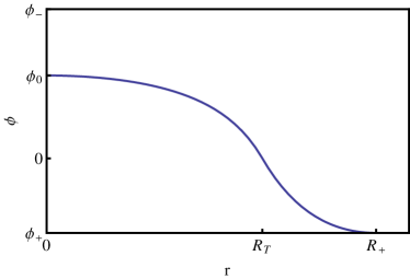
Figure 1: a) Schematic plot of the piecewise linear-quartic potential. The left part of the potential is a linear function of $\phi$, the right part a quartic function. The bounce describes tunneling from the field sitting in the false vacuum at $\phi_{+}$ towards the true vacuum located at $\phi_{-}$. b) Schematic view of the bounce solution for (a). Inside the bubble at $r=0$, the field is at $\phi_{0}>0$. The bubble wall is located around $R_{T}$, but not necessarily thin. Outside of the bubble at $r=R_{+}$, the field is still in the false vacuum.

Subject to the boundary conditions $\phi_{R}(0)=\phi_{0},\phi_{R}^{\prime}(0)=0$, solving the equation of motion of the bounce, i.e. Eq. (1) on the right side of the potential, we have Dutta et al. (2011)

$$\phi_{R}(r) = \phi_{-}+\frac{2(\phi_{0}-\phi_{-})}{2-\frac{\Delta V_{-}(\phi_{0}-\phi_{-})^{2}}{\phi_{-}^{4}}r^{2}}\,.$$ (6)

Similarly on the left side of the potential, subject to $\phi_{L}(R_{+})=\phi_{+},\phi_{L}^{\prime}(R_{+})=0$, we have the bounce solution

$$\phi_{L}(r) = \phi_{+}-\frac{\Delta V_{+}}{8\phi_{+}}\frac{(r^{2}-R_{+}^{2})^{2}}{r^{2}}\,.$$ (7)

A schematic view of the bounce is shown in Figure 1 b).

We now determine the constants $R_{+}$ and $\phi_{0}$ by solving the matching equations for the two solutions $\phi_{R}(R_{T})=0,\,\phi_{L}(R_{T})=0$. Using the first condition, we get $\phi_{0}$ in terms of $R_{T}$

$$\phi_{0} = \frac{\phi_{-}^{3}}{\Delta V_{-}R_{T}^{2}}\left[\frac{\Delta V_{-}R_{T}^{2}}{\phi_{-}^{2}}+\left(1-\sqrt{\frac{2\Delta V_{-}R_{T}^{2}}{\phi_{-}^{2}}+1}\right)\right]\,,$$ (8)

while the second condition gives

$$R_{+} = \sqrt{R_{T}\left(R_{T}+\frac{2\sqrt{2}\alpha\phi_{-}}{\sqrt{\Delta\Delta V_{-}}}\right)}\,.$$ (9)

Here, we have introduced $\Delta=\Delta V_{+}/\Delta V_{-}$ and $\alpha=-\phi_{+}/\phi_{-}$. Similarly, using the smoothness of the solution at $R_{T}$, i.e. $\phi_{R}^{\prime}(R_{T})=\phi_{L}^{\prime}(R_{T})$, we find

$$R_{T}=\frac{\phi_{-}\left(\sqrt{\Delta}(1+2\alpha)+\sqrt{4\alpha(1+\alpha)+\Delta}\right)}{(1-\Delta)\sqrt{2\Delta V_{-}}}\,.$$ (10)

Computing the exponent of the tunneling amplitude in terms of $R_{T}$ gives

$$B = \frac{\pi^{2}}{6\Delta V_{-}}\left\{3R_{T}^{4}\left(\Delta-1\right)\Delta V_{-}^{2}+8\sqrt{2}R_{T}^{3}\alpha\Delta V_{-}\sqrt{\Delta\Delta V_{-}}\phi_{-}+2\phi_{-}^{4}\left[-1+\sqrt{1+\frac{2R_{T}^{2}\Delta V_{-}}{\phi_{-}^{2}}}\right]\right.$$ (11)

$$\phantom{bla}\left.+2R_{T}^{2}\Delta V_{-}\phi_{-}^{2}\left[(6\alpha^{2}-3)+2\sqrt{1+\frac{2R_{T}^{2}\Delta V_{-}}{\phi_{-}^{2}}}\right]\right\}\,.$$

Plugging $R_{T}$ from Eq. (10), we obtain a rather monstrous expression

$$B = \frac{\pi^{2}\phi_{-}^{4}}{6\Delta V_{-}}\Bigg{\{}4\alpha\sqrt{\Delta}\left[\frac{(1+2\alpha)\sqrt{\Delta}+\sqrt{4\alpha(1+\alpha)+\Delta}}{1-\Delta}\right]^{3}-\frac{3}{4}\left[\frac{(1+2\alpha)\sqrt{\Delta}+\sqrt{4\alpha(1+\alpha)+\Delta}}{(1-\Delta)^{3/4}}\right]^{4}$$ (12)

$$\phantom{bla}+\left[\frac{(1+2\alpha)\sqrt{\Delta}+\sqrt{4\alpha(1+\alpha)+\Delta}}{1-\Delta}\right]^{2}\left[-3+6\alpha^{2}+2\sqrt{1+\left[\frac{(1+2\alpha)\sqrt{\Delta}+\sqrt{4\alpha(1+\alpha)+\Delta}}{1-\Delta}\right]^{2}}\right]$$

$$\phantom{bla}+2\left[-1+\sqrt{1+\left[\frac{(1+2\alpha)\sqrt{\Delta}+\sqrt{4\alpha(1+\alpha)+\Delta}}{1-\Delta}\right]^{2}}\right]\Bigg{\}}\,.$$

To cross check our result, we take the thin-wall limit of Eq. (12) by replacing $\Delta=1-\frac{\epsilon}{\Delta V_{-}}$, where $\epsilon$ is the energy difference between the true and false vacua. In the thin-wall limit $\epsilon\ll V_{T}$. Performing a series expansion around $\epsilon=0$, the lowest order term in $\epsilon$ is

$$\lim_{\epsilon\to 0}B=\frac{2\pi^{2}}{3}\frac{(1+2\alpha)^{4}\phi_{-}^{4}\Delta V_{-}^{2}}{\epsilon^{3}}\,.$$ (13)

We compare this with the results obtained using the thin wall approximation Coleman (1977)

$$B_{TW} \equiv \frac{27\pi^{2}}{2}\frac{S_{1}^{4}}{\epsilon^{3}}\,,$$ (14)

where

$$S_{1} \equiv \int_{\phi_{-}}^{\phi_{+}}\!d\phi\sqrt{2\left(V(\phi)-V(\phi_{+})\right)}=-\frac{\sqrt{2\Delta V_{-}}\phi_{-}}{3}\left[(1+2\alpha)\sqrt{\Delta}+2\sqrt{\Delta-1}\,_{2}F_{1}\left(\frac{1}{4},\frac{1}{2},\frac{5}{4},\frac{1}{1-\Delta}\right)\right]\,,$$ (15)

with hypergeometric function ${}_{2}F_{1}$. Again, replacing $\Delta=1-\frac{\epsilon}{\Delta V_{-}}$ gives to the lowest order in $\epsilon$

$$B_{TW} \approx \frac{2\pi^{2}}{3}\frac{(1+2\alpha)^{4}\phi_{-}^{4}\Delta V_{-}^{2}}{\epsilon^{3}}\,,$$ (16)

in agreement with Eq. (13).

As another cross-check, we observe that for fixed $\Delta$ and $\phi_{+}$, sending $|\phi_{-}|\ll|\phi_{+}|$, the potential on the right appears more and more like a linear potential. In other words, in the limit of $\alpha\gg 1$, the tunneling bounce action in Eq. (12) must agree with the tunneling bounce action in a piecewise linear-linear potential. The exact tunneling amplitude for a piecewise linear-linear potential has been calculated by Duncan and Jensen Duncan and Jensen (1992). In our notation, their result for $\alpha>1$ is given by

$$B_{DJ} = \frac{2\pi^{2}}{3}\left(\frac{1+\alpha}{\sqrt{\Delta}-1}\right)^{3}\frac{\phi_{-}^{4}}{\Delta V_{-}}\left[(\alpha-3)\sqrt{\Delta}+1-3\alpha\right]\,.$$ (17)

In the limit of large $\alpha\gg 1$, i.e. for $|\phi_{-}|\ll|\phi_{+}|$, this becomes

$$\lim_{\alpha\to\infty}B_{DJ} = \frac{2\pi^{2}}{3}\frac{\alpha^{4}(\sqrt{\Delta}-3)}{(\sqrt{\Delta}-1)^{3}}\frac{\phi_{-}^{4}}{\Delta V_{-}}\,,$$ (18)

which indeed agrees with the corresponding limit of Eq. (12). Note that this is independent of the thin-wall limit.

As an aside, we observe some curious systematic behavior: the radius of the bubble in the thin-wall limit for a piecewise linear-quartic potential is given by

$$R_{T}=\frac{3S_{1}}{\epsilon}=(1+2\alpha)\frac{\sqrt{2\Delta V_{-}}\phi_{-}}{\epsilon}\,.$$ (19)

For a cubic potential for $V_{R}(\phi)$ on the right, the thin-wall approximation gives

$$R_{T} = \left(\frac{6}{5}+2\alpha\right)\frac{\sqrt{2\Delta V_{-}}\phi_{-}}{\epsilon}\,.$$ (20)

Finally, for $V_{R}(\phi)$ a quadratic potential, the bubble radius is given by Dutta et al. (2011)

$$R_{T}=\left(\frac{3}{2}+2\alpha\right)\frac{\sqrt{2\Delta V_{-}}\phi_{-}}{\epsilon}.$$ (21)

Thus we find that in the thin wall approximation, the nucleated bubble size shrinks mildly as the power of the monomials for potential in the exiting part (near the true vacuum) becomes larger.

III Quartic on the left and quartic on the right

In this section, we compute the bounce solution for tunneling from the false vacuum in a quartic potential to the true minimum in another quartic potential, see Figure 2a).

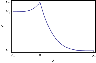
a) b)

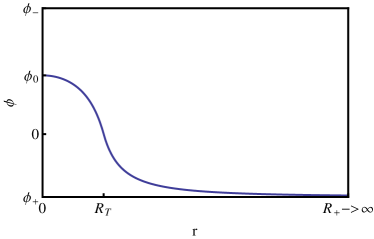
Figure 2: a) Schematic view of a piecewise quartic-quartic potential. b) Schematic view of the bounce solution for a). Note that the position where the field is still in the false vacuum goes to infinity, $R_{+}\rightarrow\infty$.

We can reuse parts of the previous calculation, in particular the solution inside the bubble from Eq. (6) and Eq. (8). Outside of the bubble, the field sits in the false vacuum

$$\phi_{L}(R_{+}) = \phi_{+}\quad\phi_{L}^{\prime}(R_{+})=0\,.$$ (22)

Note that, if we are not interested in knowing the width of the bubble, the boundary conditions above can also be set at $r\to\infty$. It turns out that this is what we need to do. The solution $\phi_{L}(r)$ has the form

$$\phi_{L}(r) = \phi_{+}+\frac{8A}{8-\frac{4\Delta\Delta V_{-}A^{2}r^{2}}{\phi_{+}^{4}}}\,,$$ (23)

with $A$ to be fixed by the condition that $\phi_{L}(R_{T})=0$. Thus we find

$$\phi_{L}(r) = \frac{\left(r^{2}-R_{T}^{2}\right)\alpha\phi_{-}\left(\frac{\Delta R_{T}^{2}\Delta V_{-}}{\alpha^{2}\phi_{-}^{2}}+\left(1+\sqrt{\frac{2\Delta R_{T}^{2}\Delta V_{-}}{\alpha^{2}\phi_{-}^{2}}+1}\right)\right)}{\Delta R_{T}^{2}\alpha^{2}\frac{\Delta R_{T}^{2}\Delta V_{-}}{\alpha^{2}\phi_{-}^{2}}-r^{2}\left(\frac{\Delta R_{T}^{2}\Delta V_{-}}{\alpha^{2}\phi_{-}^{2}}+\left(1+\sqrt{\frac{2\Delta R_{T}^{2}\Delta V_{-}}{\alpha^{2}\phi_{-}^{2}}+1}\right)\right)}\,.$$ (24)

From the smoothness of the solution $\phi_{L}^{\prime}(R_{T})=\phi_{R}^{\prime}(R_{T})\,$ we obtain

$$R_{T} = \frac{\sqrt{2(1+\alpha)(\alpha+\Delta)}}{1-\Delta}\frac{\phi_{-}}{\sqrt{V_{-}}}\,.$$ (25)

Integrating the Euclidean action gives

$$B = \frac{2\pi^{2}}{3}\frac{4\alpha^{3}+6\alpha^{2}\Delta+4\alpha\Delta^{2}+\Delta^{3}+\alpha^{4}(3+\Delta(\Delta-3))}{(1-\Delta)^{3}}\frac{\phi_{-}^{4}}{\Delta V_{-}}\,,$$ (26)

which in the thin-wall limit reduces to

$$B \approx \frac{2\pi^{2}}{3}\frac{(1+\alpha)^{4}\Delta V_{-}^{2}\phi_{-}^{4}}{\epsilon^{3}}\,.$$ (27)

Using the thin wall formula we find

$$S_{1} = -\frac{\sqrt{2\Delta V_{-}}}{3}\left[(1+\alpha)\sqrt{\Delta}+2\sqrt{(\Delta-1)}\,_{2}F_{1}\left(\frac{1}{4},\frac{1}{2},\frac{5}{4},\frac{1}{1-\Delta}\right)\right]\,,$$ (28)

and in the small $\epsilon$ limit $B$ agrees with Eq. (27).

We note that in the thin-wall limit, the tunneling bounce action $B$ for tunneling in a piecewise linear-quartic potential differs from the one in a piecewise quartic-quartic potential by the substitution $\alpha\to 2\alpha$. In particular, this means that for $\alpha\gg 1$, tunneling in a piecewise linear-quartic potential is much more suppressed than tunneling in a piecewise quartic-quartic potential: the respective values of $B$ differ by a factor of $16$, suppressing the relative amplitude by the $16^{\mathrm{th}}$ power.

a)  $B_{\text{ll}}$ $B_{\text{lq}}$ $B_{\text{qq}}$ $\alpha=0.01$ 0.0072 0.00024 0.00010 $\alpha=0.1$ 0.4 0.058 0.033 $\alpha=0.5$ 24 6.7 4.8   b)  $B_{\text{qq}}$ $B_{\text{qq, thin-wall}}$ $\Delta=0.99$ $3.3\times 10^{7}$ $3.3\times 10^{7}$ $\Delta=0.9$ $2.8\times 10^{4}$ $3.3\times 10^{4}$ $\Delta=0.7$ $7.2\times 10^{2}$ $1.2\times 10^{3}$

Table 1: a) Tunneling bounce actions for different values of $\alpha$ with $\Delta=0.01$ fixed. Tunneling in a linear-linear potential is consistently suppressed compared to tunneling in linear-quartic and quartic-quartic potentials – keeping in mind that a larger $B$ corresponds to smaller tunneling rates. b) Comparison with the thin-wall approximation for tunneling in a quartic-quartic potential for fixed $\alpha=0.5$. Decreasing $\Delta$ away from unity (i.e. exact equality between false and true vacuum energy), it is clear that the thin-wall approximation eventually fails.

To further explore the differences in tunneling rates for different potential shapes, we tabulate the values for $B$ for different values of $\alpha$, keeping $\Delta=0.01$ fixed for tunneling in a linear-linear (ll), linear-quartic (lq), and quartic-quartic (qq) potential, see Table 1. For all values of $\alpha$, the width of the wall of the nucleated bubble is non-negligible, $(R_{+}-R_{T})/R_{T}=O(1)$, so we are dealing with tunneling in the thick-wall regime. As can be seen, the action $B$ for tunneling in a linear-linear potential are always significantly larger than for tunneling in linear-quartic and quartic-quartic potentials. As the tunneling rate is proportional to $e^{-B}$, even ${\cal O}(1)$ factors lead to significant differences of the tunneling rates. In the thick-wall regime tunneling seems to depend crucially on the exact shape of the potential, making the search for more exact tunneling solutions even more pressing.

IV Conclusions

In this brief article, we discuss a quantum tunneling event in a piecewise potential where the false vacuum part is either linear or quartic and the true vacuum is described by a quartic potential. Often, the analysis of quantum tunneling in field theory is performed in the thin wall approximation Coleman (1977). This does not necessarily capture all realistic scenarios. In particular, cosmological phase transitions usually involve a large change of the energy scale. For example, the relative energy difference between neighboring vacua in the landscape of string theory is typically large. Although any specific realistic scenario can be solved by numerical methods, this makes it rather difficult to get a good qualitative understanding of the process under a change of potential parameters. As shown in the previous section, the exact shape of the potential plays a non-negligible role when considering tunneling in the thick-wall regime. Together with previous exact tunneling solutions Duncan and Jensen (1992), Hamazaki et al. (1996), Pastras (2011), Dutta et al. (2011), this work contributes to bridging the gap in qualitative understanding. As a consistency check, we have shown that the tunneling rates always reduce to the thin-wall result in the appropriate limit.

It may be appropriate at this point to outline, that our exact results here for tunneling in a piecewise linear-quartic or quartic-quartic potential can be used to describe analytically models of open inflation in a toy landscape constructed from piecewise linear and quartic potentials. The toy inflationary landscape is constructed from a piecewise linear-quartic or quartic-quartic potential, to which a slow-roll inflationary region is attached with matching $V^{\prime}$ at $\phi\simeq\phi_{-}$. The crucial point here is that the quartic potential which dominates field evolution after tunneling and before entering the slow-roll region, completely suppresses a would-be fast-roll overshoot problem in the slow-roll region. This happens because the negative spatial curvature inside the CdL bubble (once gravity is to be included Coleman and De Luccia (1980), which we – but for the negative curvature inside the bubble – do not discuss here) formed during tunneling provides a very strong friction term. This Hubble friction is sufficient for damping the downhill motion enough to start slow-roll subsequently Dutta et al. (2011) for any potential

$$V(\phi)=V_{0}+(\phi-\phi_{-})^{p}\quad,\quad p\geq 4\quad.$$ (29)

In such potentials the field will reach slow-roll already at some $\phi<\phi_{-}$ without overshoot, if the field starts its evolution inside a negatively curved CdL bubble following tunneling. Because of this fact, it does not matter whether the slow-roll inflationary region in the scalar potential at $\phi\gtrsim\phi_{-}$ will describe a small-field or large-field inflation model, as all models are treated equally in this toy landscape. We can now take a look at the situation where the barrier parameters $\alpha,\Delta$ take values in a dense discretuum specified in terms of a dense discretuum of microscopic parameters of a landscape of isolated vacua, such as the landscape of string theory vacua. For the moment, we will keep $\alpha$ fixed, as at $\alpha=0$ the scalar potential becomes discontinuous and the bounce ceases to exist. We may now assign $\Delta$, which controls the aspect of the barrier shape crossing over between the thin-wall and thick-wall limit, a prior probability distribution $p(\Delta)$. This distribution contains the unknown microscopic landscape data. As explained before, all values of $\Delta$ are treated equally when it comes to the slow-roll inflationary regime attached at $\phi\gtrsim\phi_{-}$ in our toy landscape. Therefore, the expectation value of $\Delta$ is given by

$$\langle\Delta\rangle=\frac{\int d\Delta\,p(\Delta)\,e^{-B(\Delta)}}{\int d\Delta\,p(\Delta)}\quad.$$ (30)

This does not depend on the post-tunneling inflationary dynamics due to the absence of overshoot. Therefore, in such a toy landscape the question whether the tunneling dynamics succeeds in pushing $\langle\Delta\rangle\to 0$, or whether it is overwhelmed by the prior $p(\Delta)$, is directly determined by the choice of the measure on eternal inflation entering $p(\Delta)$, and decouples from the phase space problem of post-tunneling inflation.

References

- Huber and Konstandin (2008) S. J. Huber and T. Konstandin, “Gravitational Wave Production by Collisions: More Bubbles”, JCAP 0809 (2008) 022, arXiv:0806.1828.
- Bousso and Polchinski (2000) R. Bousso and J. Polchinski, “Quantization of four form fluxes and dynamical neutralization of the cosmological constant”, JHEP 0006 (2000) 006, arXiv:hep-th/0004134.
- Susskind (2003) L. Susskind, “The Anthropic landscape of string theory”, arXiv:hep-th/0302219.
- Coleman (1977) S. R. Coleman, “The Fate of the False Vacuum. 1. Semiclassical Theory”, Phys. Rev. D15 (1977) 2929–2936.
- Coleman and De Luccia (1980) S. R. Coleman and F. De Luccia, “Gravitational Effects on and of Vacuum Decay”, Phys. Rev. D21 (1980) 3305.
- Hawking and Moss (1982) S. Hawking and I. Moss, “Supercooled Phase Transitions in the Very Early Universe”, Phys.Lett. B110 (1982) 35.
- Callan and Coleman (1977) J. Callan, Curtis G. and S. R. Coleman, “The Fate of the False Vacuum. 2. First Quantum Corrections”, Phys.Rev. D16 (1977) 1762–1768.
- Adams (1993) F. C. Adams, “General solutions for tunneling of scalar fields with quartic potentials”, Phys.Rev. D48 (1993) 2800–2805, arXiv:hep-ph/9302321.
- Duncan and Jensen (1992) M. J. Duncan and L. G. Jensen, “Exact tunneling solutions in scalar field theory”, Phys.Lett. B291 (1992) 109–114.
- Hamazaki et al. (1996) T. Hamazaki, M. Sasaki, T. Tanaka, and K. Yamamoto, “Selfexcitation of the tunneling scalar field in false vacuum decay”, Phys.Rev. D53 (1996) 2045–2061, arXiv:gr-qc/9507006.
- Pastras (2011) G. Pastras, “Exact Tunneling Solutions in Minkowski Spacetime and a Candidate for Dark Energy”, arXiv:1102.4567.
- Dutta et al. (2011) K. Dutta, P. M. Vaudrevange, and A. Westphal, “An Exact Tunneling Solution in a Simple Realistic Landscape”, arXiv:1102.4742, * Temporary entry *.
- Lee and Weinberg (1986) K.-M. Lee and E. J. Weinberg, “TUNNELING WITHOUT BARRIERS”, Nucl.Phys. B267 (1986) 181.
- Dong and Harlow (2011) X. Dong and D. Harlow, “Analytic Coleman-de Luccia Geometries”, arXiv:1109.0011.
- Dutta et al. (2011) K. Dutta, P. M. Vaudrevange, and A. Westphal, “The Overshoot Problem in Inflation after Tunneling”, arXiv:1109.5182, * Temporary entry *.