Three theorems in
discrete random geometry

Abstract

These notes are focused on three recent results in discrete random geometry, namely: the proof by Duminil-Copin and Smirnov that the connective constant of the hexagonal lattice is $\sqrt{2+\sqrt{2}}$; the proof by the author and Manolescu of the universality of inhomogeneous bond percolation on the square, triangular, and hexagonal lattices; the proof by Beffara and Duminil-Copin that the critical point of the random-cluster model on $\mathbb{Z}^{2}$ is $\sqrt{q}/(1+\sqrt{q})$. Background information on the relevant random processes is presented on route to these theorems. The emphasis is upon the communication of ideas and connections as well as upon the detailed proofs.

1 Introduction

These notes are devoted to three recent rigorous results of significance in the area of discrete random geometry in two dimensions. These results are concerned with self-avoiding walks, percolation, and the random-cluster model, and may be summarized as:

• the connective constant for self-avoiding walks on the hexagonal lattice is $\sqrt{2+\sqrt{2}}$, [15].

• the universality of inhomogeneous bond percolation on the square, triangular and hexagonal lattices, [24],

• the critical point of the random-cluster model on the square lattice with cluster-weighting factor $q\geq 1$ is $\sqrt{q}/(1+\sqrt{q})$, [7].

In each case, the background and context will be described and the theorem stated. A complete proof is included in the case of self-avoiding walks, whereas reasonably detailed outlines are presented in the other two cases.

If the current focus is on three specific theorems, the general theme is two-dimensional stochastic systems. In an exciting area of current research initiated by Schramm [55, 56], connections are being forged between discrete models and conformality; we mention percolation [60], the Ising model [14], uniform spanning trees and loop-erased random walk [47], the discrete Gaussian free field [57], and self-avoiding walks [16]. In each case, a scaling limit leads (or will lead) to a conformal structure characterized by a Schramm–Löwner evolution (SLE). In the settings of (a), (b), (c) above, the relevant scaling limits are yet to be proved, and in that sense this article is about three ‘pre-conformal’ families of stochastic processes.

There are numerous surveys and books covering the history and basic methodology of these processes, and we do not repeat this material here. Instead, we present clear definitions of the processes in question, and we outline those parts of the general theory to be used in the proofs of the above three theorems. Self-avoiding walks (SAWs) are the subject of Section 2, bond percolation of Section 3, and the random-cluster model of Section 4. More expository material about these three topics may be found, for example, in [22], as well as: SAWs [49]; percolation [10, 20, 66]; the random-cluster model [21, 67]. The relationship between SAWs, percolation, and SLE is sketched in the companion paper [46]. Full references to original material are not invariably included.

A balance is attempted in these notes between providing enough but not too much basic methodology. One recurring topic that might delay readers is the theory of stochastic inequalities. Since a sample space of the form $\Omega=\{0,1\}^{E}$ is a partially ordered set, one may speak of increasing random variables. This in turn gives rise to a partial order on probability measures on $\Omega$ by: $\mu\leq_{\text{\rm st}}\mu^{\prime}$ if $\mu(X)\leq\mu^{\prime}(X)$ for all increasing random variables $X$. Holley’s theorem [31] provides a useful sufficient criterion for such an inequality in the context of this article. The reader is referred to [21, Chap. 2] and [22, Chap. 4] for accounts of Holley’s theorem, as well as of ‘positive association’ and the FKG inequality.

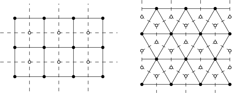
Figure 1.1: The square lattice $\mathbb{L}^{2}$ and its dual square lattice. The triangular lattice $\mathbb{T}$ and its dual hexagonal (or ‘honeycomb’) lattice $\mathbb{H}$.

A variety of lattices will be encountered in this article, but predominantly the square, triangular, and hexagonal lattices illustrated in Figure 1.1. More generally, a lattice in $d$ dimensions is a connected graph ${\mathcal{L}}$ with bounded vertex-degrees, together with an embedding in $\mathbb{R}^{d}$ such that: the embedded graph is locally-finite and invariant under shifts of $\mathbb{R}^{d}$ by any of $d$ independent vectors $\tau_{1},\tau_{2},\dots,\tau_{d}$. We shall sometimes speak of a lattice without having regard to its embedding. A lattice is vertex-transitive if, for any pair $v$, $w$ of vertices, there exists a graph-automorphism of ${\mathcal{L}}$ mapping $v$ to $w$. For simplicity, we shall consider only vertex-transitive lattices. We pick some vertex of a lattice ${\mathcal{L}}$ and designate it the origin, denoted $0$, and we generally assume that $0$ is embedded at the origin of $\mathbb{R}^{d}$. The degree of a vertex-transitive lattice is the number of edges incident to any given vertex. We write $\mathbb{L}^{d}$ for the $d$-dimensional (hyper)cubic lattice, and $\mathbb{T}$, $\mathbb{H}$ for the triangular and hexagonal lattices.

2 Self-avoiding walks

2.1 Background

Let ${\mathcal{L}}$ be a lattice with origin $0$, and assume for simplicity that ${\mathcal{L}}$ is vertex-transitive. A self-avoiding walk (SAW) is a lattice path that visits no vertex more than once.

How many self-avoiding walks of length $n$ exist, starting from the origin? What is the ‘shape’ of such a SAW chosen at random? In particular, what can be said about the distance between its endpoints? These and related questions have attracted a great deal of attention since the notable paper [26] of Hammersley and Morton, and never more so than in recent years. Mathematicians believe but have not proved that a typical SAW on a two-dimensional lattice ${\mathcal{L}}$, starting at the origin, converges in a suitable manner as $n\to\infty$ to a SLE_8/3 curve. See [16, 49, 56, 61] for discussion and results.

Paper [26] contained a number of stimulating ideas, of which we mention here the use of subadditivity in studying asymptotics. This method and its elaborations have proved extremely fruitful in many contexts since. Let ${\mathcal{S}}_{n}$ be the set of SAWs with length $n$ starting at the origin, with cardinality $\sigma_{n}=\sigma_{n}({\mathcal{L}}):=|{\mathcal{S}}_{n}|$.

Lemma 2.1 ([26]).

We have that $\sigma_{m+n}\leq\sigma_{m}\sigma_{n}$, for $m,n\geq 0$.

Proof.

Let $\pi$ and $\pi^{\prime}$ be finite SAWs starting at the origin, and denote by $\pi\ast\pi^{\prime}$ the walk obtained by following $\pi$ from 0 to its other endpoint $x$, and then following the translated walk $\pi^{\prime}+x$. Every $\nu\in{\mathcal{S}}_{m+n}$ may be written in a unique way as $\nu=\pi\ast\pi^{\prime}$ for some $\pi\in{\mathcal{S}}_{m}$ and $\pi^{\prime}\in{\mathcal{S}}_{n}$. The claim of the lemma follows. ∎

Theorem 2.2.

Let ${\mathcal{L}}$ be a vertex-transitive lattice in $d\geq 2$ dimensions with degree $\Delta$. The limit $\kappa=\kappa({\mathcal{L}})=\lim_{n\to\infty}(\sigma_{n})^{1/n}$ exists and satisfies $1<\kappa\leq\Delta-1$.

Proof.

By Lemma 2.1, $x_{m}=\log\sigma_{m}$ satisfies the ‘subadditive inequality’

$$x_{m+n}\leq x_{m}+x_{n}.$$

By the subadditive-inequality theorem (see [20, App. I]), the limit

$$\lambda=\lim_{n\to\infty}\frac{1}{n}x_{n}$$

exists, and we write $\kappa=e^{\lambda}$.

Since there are at most $\Delta-1$ choices for each step of a SAW (apart from the first), we have that $\sigma_{n}\leq\Delta(\Delta-1)^{n-1}$, giving that $\kappa\leq\Delta-1$. It is left as an exercise to show $\kappa>1$. ∎

The constant $\kappa=\kappa({\mathcal{L}})$ is called the connective constant of the lattice ${\mathcal{L}}$. The exact value of $\kappa=\kappa(\mathbb{L}^{d})$ is unknown for every $d\geq 2$, see [32, Sect. 7.2, pp. 481–483]. As explained in the next section, the hexagonal lattice has a special structure which permits an exact calculation, and our main purpose here is to present the proof of this. In addition, we include next a short discussion of critical exponents, for a fuller discussion of which the reader is referred to [2, 49, 59]

By Theorem 2.2, $\sigma_{n}$ grows exponentially in the manner of $\kappa^{n(1+\text{\rm o}(1))}$. It is believed by mathematicians and physicists that there is a power-order correction, in that

$$\sigma_{n}\sim A_{1}n^{\gamma-1}\kappa^{n},$$

where the exponent $\gamma$ depends only on the number of dimensions and not otherwise on the lattice (here and later, there should be an additional logarithmic correction in four dimensions). Furthermore, it is believed that $\gamma=\frac{43}{32}$ in two dimensions. We mention two further critical exponents. It is believed that the (random) end-to-end distance $D_{n}$ of a typical $n$-step SAW satisfies

$$E(D_{n}^{2})\sim A_{2}n^{2\nu},$$

and furthermore $\nu=\frac{3}{4}$ in two dimensions. Finally, let $Z_{v}(x)=\sum_{k}\sigma_{k}(v)x^{k}$ where $\sigma_{k}(v)$ is the number of $k$-step SAWs from the origin to the vertex $v$. The generating function $Z_{v}$ has radius of convergence $\kappa^{-1}$, and it is believed that

$$Z_{v}(\kappa^{-1})\sim A_{3}|v|^{-(d-2+\eta)}\qquad\text{as }|v|\to\infty,$$

in $d$ dimensions. Furthermore, $\eta$ should satisfy the so-called Fisher relation $\gamma=(2-\eta)\nu$, giving that $\eta=\frac{5}{24}$ in two dimensions. The numerical predictions for these exponents in two dimensions are explicable on the conjectural basis that a typical $n$-step SAW in two dimensions converges to SLE_8/3 as $n\to\infty$ (see [6, 48]).

2.2 Hexagonal-lattice connective constant

Theorem 2.3 ([15]).

The connective constant of the hexagonal lattice $\mathbb{H}$ satisfies $\kappa(\mathbb{H})=\sqrt{2+\sqrt{2}}$.

This result of Duminil-Copin and Smirnov provides a rigorous and provocative verification of a prediction of Nienhuis [50] based on conformal field theory. The proof falls short of a proof of conformal invariance for self-avoiding walks on $\mathbb{H}$. The remainder of this section contains an outline of the proof of Theorem 2.3, and is drawn from [15].

The reader may wonder about the special nature of the hexagonal lattice. It is something of a mystery why certain results for this lattice (for example, Theorem 2.3, and the conformal scaling limit of ‘face’ percolation) do not yet extend to other lattices.

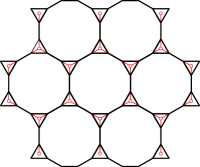
Figure 2.1: The Archimedean lattice $(3,12^{2})$ is obtained by replacing each vertex of the hexagonal lattice $\mathbb{H}$ by a triangle.

We note an application of Theorem 2.3 to the lattice illustrated in Figure 2.1, namely the Archimedean lattice denoted $\mathbb{A}=(3,12^{2})$ and known also as a ‘Fisher lattice’ after [17]. Edges of $\mathbb{A}$ lying in a triangle are called triangular. For simplicity, we shall consider only SAWs of $\mathbb{A}$ that start with a triangular edge and finish with a non-triangular edge. The non-triangular edges of such a SAW $a$ induce a SAW $h$ of $\mathbb{H}$. Furthermore, for given $h$, the corresponding $a$ are obtained by replacing each vertex $v$ of $h$ (other than its final vertex) by either a single edge in the triangle of $\mathbb{A}$ at $v$, or by two such edges. It follows that the generating function of such walks is

$$Z^{\mathbb{A}}(a)=\sum_{k}\sigma_{k}(\mathbb{H})(a^{2}+a^{3})^{k}=Z(a^{2}+a^{3}),$$

where $Z(x):=\sum_{n}\sigma_{n}(\mathbb{H})x^{k}$. The radius of convergence of $Z^{\mathbb{A}}$ is $1/\kappa(\mathbb{A})$, and we deduce the following formula of [33]:

$$\frac{1}{\kappa(\mathbb{A})^{2}}+\frac{1}{\kappa(\mathbb{A})^{3}}=\frac{1}{\kappa(\mathbb{H})}.$$ (2.1)

One may show similarly that the critical exponents $\gamma$, $\nu$, $\eta$ are equal for $\mathbb{A}$ and $\mathbb{H}$, assuming they satisfy suitable definitions. The details are omitted.

Proof of Theorem 2.3.

This exploits the relationship between $\mathbb{R}^{2}$ and the Argand diagram of the complex numbers $\mathbb{C}$. We embed $\mathbb{H}=(V,E)$ in $\mathbb{R}^{2}$ in a natural way: edges have length 1 and are inclined at angles $\pi/6$, $\pi/2$, $5\pi/6$ to the $x$-axis, the origins of ${\mathcal{L}}$ and $\mathbb{R}^{2}$ coincide, and the line-segment from $(0,0)$ to $(0,1)$ is an edge of $\mathbb{H}$. Any point in $\mathbb{H}$ may thus be represented by a complex number. Let ${\mathcal{M}}$ be the set of midpoints of edges of $\mathbb{H}$. Rather than counting paths between vertices of $\mathbb{H}$, we count paths between midpoints.

Fix $a\in{\mathcal{M}}$, and let

$$Z(x)=\sum_{\gamma}x^{|\gamma|},\qquad x\in(0,\infty),$$

where the sum is over all SAWs $\gamma$ starting at $a$, and $|\gamma|$ is the number of vertices visited by $\gamma$. Theorem 2.3 is equivalent to the assertion that the radius of convergence of $Z$ is $\chi:=1/\sqrt{2+\sqrt{2}}$. We shall therefore prove that

$$Z(\chi) =\infty,$$ (2.2)

$$Z(x) <\infty\quad\text{ for }x<\chi.$$ (2.3)

Towards this end we introduce a function that records the turning angle of a SAW. A SAW $\gamma$ departs from its starting-midpoint $a$ in one of two possible directions, and its direction changes by $\pm\pi/3$ at each vertex. On arriving at its other endpoint $b$, it has turned through some total turning angle $T(\gamma)$, measured anticlockwise in radians.

We work within some bounded region $M$ of $\mathbb{H}$. Let $S\subseteq V$ be a finite set of vertices that induces a connected subgraph, and let $M=M_{S}$ be the set of midpoints of edges touching points in $S$. Let $\Delta M$ be the set of midpoints for which the corresponding edge of $\mathbb{H}$ has exactly one endpoint in $S$. Later in the proof we shall restrict $M$ to a region of the type illustrated in Figure 2.2.

Figure 2.2: The region $M_{h,v}$ has $2h+1$ midpoints on the bottom side, and $v$ at the left/right sides. In this illustration, we have $h=2$ and $v=5$.

Let $a\in\Delta M$ and $\sigma,x\in(0,\infty)$, and define the so-called ‘parafermionic observable’ of [15] by

$$F_{a,M}^{\sigma,x}(z)=\sum_{\gamma:a\to z}e^{-i\sigma T(\gamma)}x^{|\gamma|},\qquad z\in M,$$ (2.4)

where the summation is over all SAWs from $a$ to $z$ lying entirely in $M$. We shall suppress some of the notation in $F_{a,M}^{\sigma,x}$ when no ambiguity ensues. The key ingredient of the proof is the following lemma, which is strongly suggestive of discrete analyticity.

Lemma 2.4.

Let $\sigma=\frac{5}{8}$ and $x=\chi$. For $v\in S$,

$$(p-v)F(p)+(q-v)F(q)+(r-v)F(r)=0,$$ (2.5)

where $p,q,r\in{\mathcal{M}}$ are the midpoints of the three edges incident to $v$.

The quantities in (2.5) are to be interpreted as complex numbers.

Proof of Lemma 2.4.

Let $v\in S$. We assume for definiteness that the star at $v$ is as drawn on the left of Figure 2.3.

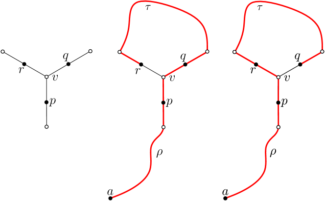
Figure 2.3: The star centred at the vertex $v$ is on the left. Two SAWs lying in ${\mathcal{P}}_{3}$, visiting the midpoints of edges in the respective orders $pqr$ and $prq$. They follow the same SAWs $\rho$ and $\tau$ (in one or the other directions), and differ only within the star.

Let ${\mathcal{P}}_{k}$ be the set of SAWs of $M$ starting at $a$ whose intersection with $\{p,q,r\}$ has cardinality $k$, for $k=1,2,3$. We shall show that the aggregate contribution to (2.5) of ${\mathcal{P}}_{1}\cup{\mathcal{P}}_{2}$ is zero, and similarly of ${\mathcal{P}}_{3}$.

Consider first ${\mathcal{P}}_{3}$. Let $\gamma\in{\mathcal{P}}_{3}$, and write $b_{1}$, $b_{2}$, $b_{3}$ for the ordering of $\{p,q,r\}$ encountered along $\gamma$ starting at $a$. Thus $\gamma$ comprises:

• a SAW $\rho$ from $a$ to $b_{1}$,

• a SAW of length 1 from $b_{1}$ to $b_{2}$,

• a SAW $\tau$ from $b_{2}$ to $b_{3}$ that is disjoint from $\rho$,

as illustrated in Figure 2.3. We partition ${\mathcal{P}}_{3}$ according to the pair $\rho$, $\tau$. For given $\rho$, $\tau$, the aggregate contribution of these two paths to the left side of (2.5) is

$$c\left(\overline{\theta}e^{-i\sigma 4\pi/3}+\theta e^{i\sigma 4\pi/3}\right)$$ (2.6)

where $c=(b_{1}-v)e^{-i\sigma T(\rho)}x^{|\rho|+|\tau|+1}$ and

$$\theta=\frac{q-v}{p-v}=e^{i2\pi/3}.$$

The parenthesis in (2.6) equals $2\cos\bigl{(}\frac{2}{3}\pi(2\sigma+1)\bigr{)}$ which is $0$ when $\sigma=\frac{5}{8}$.

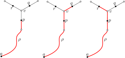
Figure 2.4: The left SAW, denoted $\gamma_{p}$, intersects the set $\{p,q,r\}$ once only. The other two paths, denoted $\gamma_{q}$ and $\gamma_{r}$, are extensions of the first.

Consider now ${\mathcal{P}}_{1}\cup{\mathcal{P}}_{2}$. This set may be partitioned according to the point $b$ in $\{p,q,r\}$ visited first, and by the route $\rho$ of the SAW from $a$ to $b$. For given $b$, $\rho$, there are exactly three such SAWs, as in Figure 2.4. Their aggregate contribution to the left side of (2.5) is

$$c\left(1+x\theta e^{i\sigma\pi/3}+x\overline{\theta}e^{-i\sigma\pi/3}\right)$$

where $c=(b-v)e^{-i\sigma T(\gamma_{b})}x^{|\gamma_{b}|}$. With $\sigma=\frac{5}{8}$, we set this to $0$ and solve for $x$, to find $x=1/[2\cos(\pi/8)]=\chi$. The lemma is proved. ∎

We return to the proof of Theorem 2.3, and we set $\sigma=\frac{5}{8}$ henceforth. Let $M=M_{h,v}$ be as in Figure 2.2, and let $L_{h}$, $T^{\pm}_{h,v}$, $U_{h,v}$ be the sets of midpoints indicated in the figure (note that $a$ is excluded from $L_{h}$). Let

$$\lambda^{x}_{h,v}=\sum_{\gamma:a\to L_{h}}x^{|\gamma|},$$

where the sum is over all SAWs in $M_{h,v}$ from $a$ to some point in $L_{h}$. All such $\gamma$ have $T(\gamma)=\pm\pi$. The sums $\tau^{\pm,x}_{h,v}$ and $\zeta_{h,v}^{x}$ are defined similarly in terms of SAWs ending in $T^{\pm}_{h,v}$ and $U_{h,v}$ respectively, and all such $\gamma$ have $T(\gamma)=\mp 2\pi/3$ and $T(\gamma)=0$ respectively.

In summing (2.5) over all vertices $v$ of $M_{h,v}$, with $x=\chi$, all contributions cancel except those from the boundary midpoints. Using the symmetry of $M_{h,v}$, we deduce that

$$-iF^{\chi}(a)-i\Re(e^{i\sigma\pi})\lambda^{\chi}_{h,v}+i\theta e^{-i\sigma 2\pi/3}\tau^{-,\chi}_{h,v}+i\zeta^{\chi}_{h,v}+i\overline{\theta}e^{i\sigma 2\pi/3}\tau^{+,\chi}_{h,v}=0.$$

Divide by $i$, and use the fact that $F^{\chi}(a)=1$, to obtain

$$c_{l}\lambda^{\chi}_{h,v}+c_{t}\tau^{\chi}_{h,v}+\zeta^{\chi}_{h,v}=1,$$ (2.7)

where $\tau_{h,v}=\tau^{+}_{h,v}+\tau^{-}_{h,v}$, $c_{l}=\cos(3\pi/8)$, and $c_{t}=\cos(\pi/4)$.

Let $x\in(0,\infty)$. Since $\lambda^{x}_{h,v}$ and $\zeta^{x}_{h,v}$ are increasing in $h$, the limits

$$\lambda^{x}_{v}=\lim_{h\to\infty}\lambda^{x}_{h,v},\quad\zeta^{x}_{v}=\lim_{h\to\infty}\zeta^{x}_{h,v},$$

exist. Hence, by (2.7), the decreasing limit

$$\tau^{\chi}_{h,v}\downarrow\tau^{\chi}_{v}\qquad\text{as }h\to\infty,$$ (2.8)

exists also. Furthermore, by (2.7),

$$c_{l}\lambda^{\chi}_{v}+c_{t}\tau^{\chi}_{v}+\zeta^{\chi}_{v}=1.$$ (2.9)

We shall use (2.8)–(2.9) to prove (2.2)–(2.3) as follows.

Proof of (2.2). There are two cases depending on whether or not

$$\tau_{v}^{\chi}>0\qquad\text{for some }v\geq 1.$$ (2.10)

Assume first that (2.10) holds, and pick $v\geq 1$ accordingly. By (2.8), $\tau^{\chi}_{h,v}\geq\tau_{v}^{\chi}$ for all $h$, so that

$$Z(\chi)\geq\sum_{h=1}^{\infty}\tau^{\chi}_{h,v}=\infty,$$

and (2.2) follows.

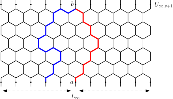
Figure 2.5: A SAW contributing to $\lambda^{\chi}_{v+1}$ but not $\lambda^{\chi}_{v}$ is broken at its first highest vertex into two SAWs coloured red and blue. By adding two half-edges, we obtain two SAWs from $b\in U_{\infty,v+1}$ to $L_{\infty}$.

Assume now that (2.10) is false so that, by (2.9),

$$c_{l}\lambda^{\chi}_{v}+\zeta^{\chi}_{v}=1,\qquad v\geq 1.$$ (2.11)

We propose to bound $Z(\chi)$ below in terms of the $\zeta^{\chi}_{v}$. The difference $\lambda^{\chi}_{v+1}-\lambda^{\chi}_{v}$ is the sum of $\chi^{|\gamma|}$ over all $\gamma$ from $a$ to $L_{\infty}$ whose highest vertex lies between $U_{\infty,v}$ and $U_{\infty,v+1}$. See Figure 2.5. We split such a $\gamma$ into two pieces at its first highest vertex, and add two half-edges to obtain two self-avoiding paths from a given midpoint, $b$ say, of $U_{\infty,v+1}$ to $L_{\infty}\cup\{a\}$. Therefore,

$$\lambda^{\chi}_{v+1}-\lambda^{\chi}_{v}\leq\chi(\zeta^{\chi}_{v+1})^{2},\qquad v\geq 1.$$

By (2.11),

$$c_{l}\chi(\zeta^{\chi}_{v+1})^{2}+\zeta^{\chi}_{v+1}\geq\zeta^{\chi}_{v},\qquad v\geq 1,$$

whence, by induction,

$$\zeta^{\chi}_{v}\geq\frac{1}{v}\min\left\{\zeta^{\chi}_{1},\frac{1}{c_{l}\chi}\right\},\qquad v\geq 1.$$

Therefore,

$$Z(\chi)\geq\sum_{v=1}^{\infty}\zeta^{\chi}_{v}=\infty.$$

Proof of (2.3). SAWs that start at a lowermost vertex and end at an uppermost vertex (or vice versa) are called bridges. Hammersley and Welsh [27] showed, as follows, that any SAW may be decomposed in a unique way into sub-walks that are bridges. They used this to obtain a bound on the rate of convergence in the limit defining the connective constant.

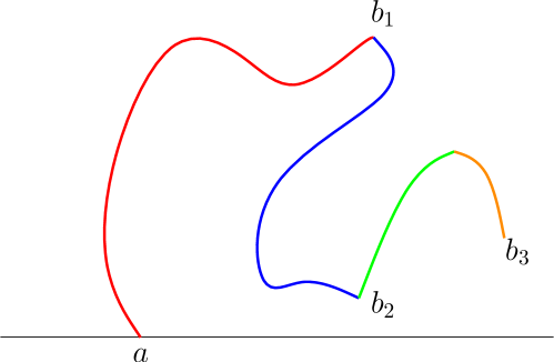
Figure 2.6: A half-plane walk $\gamma$ decomposed into four bridges.

Consider first a (finite) SAW $\gamma$ in $M_{\infty,\infty}$ starting at $a$. From amongst its highest vertices, choose the last, $b_{1}$ say. Consider the sub-walk from $b_{1}$ onwards, and find the final lowest vertex, $b_{2}$ say. Iterate the procedure until the endpoint of $\gamma$ is reached, as illustrated in Figure 2.6. The outcome is a decomposition of $\gamma$ into an ordered set of bridges with vertical displacements written $T_{0}>T_{1}>\cdots>T_{j}$.

Now let $\gamma$ be a SAW from $a$ (not necessarily a half-plane walk). Find the earliest vertex of $\gamma$ that is lowest, $c$ say. Then $\gamma$ may be decomposed into a walk $\gamma_{1}$ from $a$ to $c$, together with the remaining walk $\gamma_{2}=\gamma\setminus\gamma_{1}$. On applying the above procedure to $\gamma_{1}$ viewed backwards, we obtain a decomposition into bridges with vertical displacements written $T_{-i}<\cdots<T_{-1}$, Similarly, $\gamma_{2}$ has a decomposition with $T_{0}>\cdots>T_{j}$. The original walk $\gamma$ may be reconstructed from knowledge of the constituent bridges. A little further care is needed in our case since our walks connect midpoints rather than vertices.

One may deduce a bound for $Z(x)$ in terms of the $\zeta_{v}^{x}$. Any SAW from $a$ has two choices for initial direction, and thereafter has a bridge decomposition as above. Therefore,

$$Z(x)\leq 2\sum_{\begin{subarray}{c}T_{-i}<\cdots<T_{-1}\\ T_{0}>\cdots>T_{j}\end{subarray}}\,\prod_{k=-i}^{j}\zeta_{T_{k}}^{x}=2\prod_{T=1}^{\infty}(1+\zeta^{x}_{T})^{2}.$$ (2.12)

It remains to bound the right side.

Since all SAWs from $a$ to $U_{h,v}$ have length at least $h$,

$$\zeta^{x}_{h}\leq\left(\frac{x}{\chi}\right)^{h}\zeta^{\chi}_{h}\leq\left(\frac{x}{\chi}\right)^{h},\qquad x\leq\chi.$$

Therefore,

$$\prod_{T=1}^{\infty}(1+\zeta^{x}_{T})<\infty,\qquad x<\chi,$$

and (2.3) follows by (2.12). ∎

3 Bond percolation

3.1 Background

Percolation is the fundamental stochastic model for spatial disorder. We consider bond percolation on several lattices including the (two-dimensional) square, triangular and hexagonal lattices of Figure 1.1, and the (hyper)cubic lattices $\mathbb{L}^{d}=(\mathbb{Z}^{d},\mathbb{E}^{d})$ in $d\geq 3$ dimensions. Detailed accounts of the basic theory may be found in [20, 22].

Percolation comes in two forms, ‘bond’ and ‘site’, and we concentrate here on the bond model. Let ${\mathcal{L}}=(V,E)$ be a lattice with origin denoted 0, and let $p\in[0,1]$. Each edge $e\in E$ is designated either open with probability $p$, or closed otherwise, different edges receiving independent states. We think of an open edge as being open to the passage of some material such as disease, liquid, or infection. Suppose we remove all closed edges, and consider the remaining open subgraph of the lattice. Percolation theory is concerned with the geometry of this open graph. Of special interest is the size and shape of the open cluster $C_{0}$ containing the origin, and in particular the probability that $C_{0}$ is infinite.

The sample space is the set $\Omega=\{0,1\}^{E}$ of $0/1$-vectors $\omega$ indexed by the edge-set $E$; here, 1 represents ‘open’, and 0 ‘closed’. The probability measure is product measure $\mathbb{P}_{p}$ with density $p$.

For $x,y\in V$, we write $x\leftrightarrow y$ if there exists an open path joining $x$ and $y$. The open cluster at $x$ is the set $C_{x}=\{y:x\leftrightarrow y\}$ of all vertices reached along open paths from the vertex $x$, and we write $C=C_{0}$. The percolation probability is the function $\theta(p)$ given by

$$\theta(p)=\mathbb{P}_{p}(|C|=\infty),$$

and the critical probability is defined by

$$p_{\text{\rm c}}=p_{\text{\rm c}}({\mathcal{L}})=\sup\{p:\theta(p)=0\}.$$ (3.1)

It is elementary that $\theta$ is a non-decreasing function, and therefore,

$$\theta(p)\,\begin{cases}=0&\text{if }p<p_{\text{\rm c}},\\ >0&\text{if }p>p_{\text{\rm c}}.\end{cases}$$

It is a fundamental fact that $0<p_{\text{\rm c}}({\mathcal{L}})<1$ for any lattice ${\mathcal{L}}$ in two or more dimensions, but it is unproven in general that no infinite open cluster exists when $p=p_{\text{\rm c}}$.

Conjecture 3.1.

For any lattice ${\mathcal{L}}$ in $d\geq 2$ dimensions, we have that $\theta(p_{\text{\rm c}})=0$.

The claim of the conjecture is known to be valid for certain lattices when $d=2$ and for large $d$, currently $d\geq 19$.

Whereas the above process is defined in terms of a single parameter $p$, much of this section is directed at the multiparameter setting in which an edge $e$ is designated open with some probability $p_{e}$. In such a case, the critical probability $p_{\text{\rm c}}$ is replaced by a so-called ‘critical surface’. See Section 3.5 for a more precise discussion of this.

The theory of percolation is extensive and influential. Not only is percolation a benchmark model for studying random spatial processes in general, but also it has been, and continues to be, a source of beautiful open problems (of which Conjecture 3.1 is one). Percolation in two dimensions has been especially prominent in the last decade by virtue of its connections to conformal invariance and conformal field theory. Interested readers are referred to the papers [13, 56, 60, 61, 63, 66] and the books [10, 20, 22].

The concepts of critical exponent and scaling are discussed in Section 3.2. Section 3.3 is concerned with percolation in two dimensions, and especially the box-crossing property. The star–triangle transformation features in Section 3.4, followed by a discussion of universality in Section 3.5.

3.2 Power-law singularity

Macroscopic functions, such as the percolation probability and mean cluster-size,

$$\theta(p)=\mathbb{P}_{p}(|C|=\infty),\quad\chi(p)=\mathbb{P}_{p}(|C|),$$

have singularities at $p=p_{\text{\rm c}}$, and there is overwhelming theoretical and numerical evidence that these are of ‘power-law’ type. A great deal of effort has been directed towards understanding the nature of the percolation phase transition. The picture is now fairly clear for one specific model in $2$ dimensions (site percolation on the triangular lattice), owing to the very significant progress in recent years linking critical percolation to the Schramm–Löwner curve SLE₆. There remain however substantial difficulties to be overcome even when $d=2$, associated largely with the extension of such results to general two-dimensional systems. The case of large $d$ (currently, $d\geq 19$) is also well understood, through work based on the so-called ‘lace expansion’. Many problems remain open in the obvious case $d=3$.

The nature of the percolation singularity is expected to be canonical, in that it shares general features with phase transitions of other models of statistical mechanics. These features are sometimes referred to as ‘scaling theory’ and they relate to the ‘critical exponents’ occurring in the power-law singularities (see [20, Chap. 9]). There are two sets of critical exponents, arising firstly in the limit as $p\to p_{\text{\rm c}}$, and secondly in the limit over increasing spatial scales when $p=p_{\text{\rm c}}$. The definitions of the critical exponents are found in Table 3.1 (taken from [20]).

Table 3.1: Eight functions and their critical exponents. The first five exponents arise in the limit as $p\to p_{\text{\rm c}}$, and the remaining three as $n\to\infty$ with $p=p_{\text{\rm c}}$. See [20] for a definition of the correlation length $\xi(p)$

Function		Behaviour	Exp.
percolation	$\theta(p)=\mathbb{P}_{p}(|C|=\infty)$	$\theta(p)\approx(p-p_{\text{\rm c}})^{\beta}$	$\beta$
probability
truncated	$\chi^{\text{f}}(p)=\mathbb{P}_{p}(|C|1_{|C|<\infty})$	$\chi^{\text{f}}(p)\approx|p-p_{\text{\rm c}}|^{-\gamma}$	$\gamma$
mean cluster-size
number of	$\kappa(p)=\mathbb{P}_{p}(|C|^{-1})$	$\kappa^{\prime\prime\prime}(p)\approx|p-p_{\text{\rm c}}|^{-1-\alpha}$	$\alpha$
clusters per vertex
cluster moments	$\chi_{k}^{\text{f}}(p)=\mathbb{P}_{p}(|C|^{k}1_{|C|<\infty})$	$\displaystyle\frac{\chi_{k+1}^{\text{f}}(p)}{\chi_{k}^{\text{f}}(p)}\approx|p-p_{\text{\rm c}}|^{-\Delta}$	$\Delta$
correlation length	$\xi(p)$	$\xi(p)\approx|p-p_{\text{\rm c}}|^{-\nu}$	$\nu$
cluster volume		$\mathbb{P}_{p_{\text{\rm c}}}(|C|=n)\approx n^{-1-1/\delta}$	$\delta$
cluster radius		$\mathbb{P}_{p_{\text{\rm c}}}\bigl{(}\text{\rm rad}(C)=n\bigr{)}\approx n^{-1-1/\rho}$	$\rho$
connectivity function		$\mathbb{P}_{p_{\text{\rm c}}}(0\leftrightarrow x)\approx\|x\|^{2-d-\eta}$	$\eta$

The notation of Table 3.1 is as follows. We write $f(x)\approx g(x)$ as $x\to x_{0}\in[0,\infty]$ if $\log f(x)/\log g(x)\to 1$. The radius of the open cluster $C_{x}$ at the vertex $x$ is defined by

$$\text{\rm rad}(C_{x})=\sup\{\|y\|:x\leftrightarrow y\},$$

where

$$\|y\|=\sup_{i}|y_{i}|,\qquad y=(y_{1},y_{2},\dots,y_{d})\in\mathbb{R}^{d},$$

is the supremum ($L^{\infty}$) norm on $\mathbb{R}^{d}$. (The choice of norm is irrelevant since all norms are equivalent on $\mathbb{R}^{d}$.) The limit as $p\to p_{\text{\rm c}}$ should be interpreted in a manner appropriate for the function in question (for example, as $p\downarrow p_{\text{\rm c}}$ for $\theta(p)$, but as $p\to p_{\text{\rm c}}$ for $\kappa(p)$). The indicator function of an event $A$ is denoted $1_{A}$.

Eight critical exponents are listed in Table 3.1, denoted $\alpha$, $\beta$, $\gamma$, $\delta$, $\nu$, $\eta$, $\rho$, $\Delta$, but there is no general proof of the existence of any of these exponents for arbitrary $d\geq 2$. Such critical exponents may be defined for phase transitions in a large family of physical systems. However, it is not believed that they are independent variables, but rather that, for all such systems, they satisfy the so-called scaling relations

$$2-\alpha=\gamma+2\beta=\beta(\delta+1),$$

$$\Delta=\delta\beta,\quad\gamma=\nu(2-\eta),$$

and, when $d$ is not too large, the hyperscaling relations

$$d\rho=\delta+1,\quad 2-\alpha=d\nu.$$

More generally, a ‘scaling relation’ is any equation involving critical exponents believed to be ‘universally’ valid. The upper critical dimension is the largest value $d_{\text{\rm c}}$ such that the hyperscaling relations hold for $d\leq d_{\text{\rm c}}$. It is believed that $d_{\text{\rm c}}=6$ for percolation. There is no general proof of the validity of the scaling and hyperscaling relations for percolation, although quite a lot is known when either $d=2$ or $d$ is large. The case of large $d$ is studied via the lace expansion, and this is expected to be valid for $d>6$.

We note some further points in the context of percolation.

• Universality. The numerical values of critical exponents are believed to depend only on the value of $d$, and to be independent of the choice of lattice, and whether bond or site. Universality in two dimensions is discussed further in Section 3.5.

• Two dimensions. When $d=2$, it is believed that

  $$\alpha=-\tfrac{2}{3},\ \beta=\tfrac{5}{36},\ \gamma=\tfrac{43}{18},\ \delta=\tfrac{91}{5},\ldots$$

  These values (other than $\alpha$) have been proved (essentially only) in the special case of site percolation on the triangular lattice, see [62].

• Large dimensions. When $d$ is sufficiently large (in fact, $d\geq d_{\text{\rm c}}$) it is believed that the critical exponents are the same as those for percolation on a tree (the ‘mean-field model’), namely $\delta=2$, $\gamma=1$, $\nu=\frac{1}{2}$, $\rho=\frac{1}{2}$, and so on (the other exponents are found to satisfy the scaling relations). Using the first hyperscaling relation, this is consistent with the contention that $d_{\text{\rm c}}=6$. Several such statements are known to hold for $d\geq 19$, see [28, 29, 43].

Open challenges include the following:

• prove the existence of critical exponents for general lattices,

• prove some version of universality,

• prove the scaling and hyperscaling relations in general dimensions,

• calculate the critical exponents for general models in two dimensions,

• prove the mean-field values of critical exponents when $d\geq 6$.

Progress towards these goals has been substantial. As noted above, for sufficiently large $d$, the lace expansion has enabled proofs of exact values for many exponents. There has been remarkable progress in recent years when $d=2$, inspired largely by work of Schramm [55], enacted by Smirnov [60], and confirmed by the programme pursued by Lawler, Schramm, Werner, Camia, Newman and others to understand SLE curves and conformal ensembles.

Only two-dimensional lattices are considered in the remainder of Section 3.

3.3 Box-crossing property

Loosely speaking, the ‘box-crossing property’ is the property that the probability of an open crossing of a box with given aspect-ratio is bounded away from 0, uniformly in the position, orientation, and size of the box.

Let ${\mathcal{L}}=(V,E)$ be a planar lattice drawn in $\mathbb{R}^{2}$, and let $\mathbb{P}$ be a probability measure on $\Omega=\{0,1\}^{E}$. For definiteness, we may think of ${\mathcal{L}}$ as one of the square, triangular, and hexagonal lattices, but the following discussion is valid in much greater generality.

Let $R$ be a (non-square) rectangle of $\mathbb{R}^{2}$. A lattice-path $\pi$ is said to cross $R$ if $\pi$ contains an arc (termed a box-crossing) lying in the interior of $R$ except for its two endpoints, which are required to lie, respectively, on the two shorter sides of $R$. Note that a box-crossing of a rectangle lies in the longer direction.

Let $\omega\in\Omega$. The rectangle $R$ is said to possess an open crossing if there exists an open box-crossing of $R$, and we write $C(R)$ for this event. Let ${\mathcal{T}}$ be the set of translations of $\mathbb{R}^{2}$, and $\tau\in{\mathcal{T}}$. Fix the aspect-ratio $\rho>1$. Let $H_{n}=[0,\rho n]\times[0,n]$ and $V_{n}=[0,n]\times[0,\rho n]$, and let $n_{0}=n_{0}({\mathcal{L}})<\infty$ be minimal with the property that, for all $\tau\in{\mathcal{T}}$ and all $n\geq n_{0}$, $\tau H_{n}$ and $\tau V_{n}$ possess crossings in ${\mathcal{L}}$. Let

$$\beta_{\rho}({\mathcal{L}},\mathbb{P}) =\inf\Bigl{\{}\mathbb{P}(C(\tau H_{n})),\mathbb{P}(C(\tau V_{n})):n\geq n_{0},\ \tau\in{\mathcal{T}}\Bigr{\}}.$$ (3.2)

The pair $({\mathcal{L}},\mathbb{P})$ is said to have the $\rho$-box-crossing property if $\beta_{\rho}({\mathcal{L}},\mathbb{P})>0$.

The measure $\mathbb{P}$ is called positively associated if, for all increasing cylinder events $A$, $B$,

$$\mathbb{P}(A\cap B)\geq\mathbb{P}(A)\mathbb{P}(B).$$ (3.3)

(See [22, Sect. 4.2].) The value of $\rho$ in the box-crossing property is in fact immaterial, so long as $\rho>1$ and $\mathbb{P}$ is positively associated. We state this explicitly as a proposition since we shall need it in Section 4. The proof is left as an exercise (see [22, Sect. 5.5]).

Proposition 3.2.

Let $\mathbb{P}$ be a probability measure on $\Omega$ that is positively associated. If there exists $\rho>1$ such that $({\mathcal{L}},\mathbb{P})$ has the $\rho$-box-crossing property, then $({\mathcal{L}},\mathbb{P})$ has the $\rho$-box-crossing property  for all $\rho>1$.

It is standard that the percolation measure (and more generally the random-cluster measure of Section 4, see [21, Sect. 3.2]) are positively associated, and thus we may speak simply of the box-crossing property.

Here is a reminder about duality for planar graphs. Let $G=(V,E)$ be a planar graph, drawn in the plane. Loosely speaking, the planar dual $G_{\text{\rm d}}$ of $G$ is the graph constructed by placing a vertex inside every face of $G$ (including the infinite face if it exists) and joining two such vertices by an edge $e_{\text{\rm d}}$ if and only if the corresponding faces of $G$ share a boundary edge $e$. The edge-set $E_{\text{\rm d}}$ of $G_{\text{\rm d}}$ is in one–one correspondence ($e\leftrightarrow e_{\text{\rm d}}$) with $E$. The duals of the square, triangular, and hexagonal lattices are illustrated in Figure 1.1.

Let $\Omega=\{0,1\}^{E}$, and $\omega\in\Omega$. With $\omega$ we associate a configuration $\omega_{\text{\rm d}}$ in the dual space $\Omega_{\text{\rm d}}=\{0,1\}^{E_{\text{\rm d}}}$ by $\omega(e)+\omega_{\text{\rm d}}(e_{\text{\rm d}})=1$. Thus, an edge of the dual is open if and only if it crosses a closed edge of the primal graph. The measure $\mathbb{P}_{p}$ on $\Omega$ induces the measure $\mathbb{P}_{1-p}$ on $\Omega_{\text{\rm d}}$.

The box-crossing property is fundamental to rigorous study of percolation in two dimensions. When it holds, the process is either critical or supercritical. If both $({\mathcal{L}},\mathbb{P}_{p})$ and its dual $({\mathcal{L}}_{\text{\rm d}},\mathbb{P}_{1-p})$ have the box-crossing property, then each is critical (see, for example, [23, Props 4.1, 4.2]). The box-crossing property was developed by Russo [54], and Seymour and Welsh [58], and exploited heavily by Kesten [38]. Further details of the use of the box-crossing property may be found in [12, 60, 63, 66].

One way of estimating the chance of a box-crossing is via its derivative. Let $A$ be an increasing cylinder event, and let $g(p)=\mathbb{P}_{p}(A)$. An edge $e$ is called pivotal for $A$ (in a configuration $\omega$) if $\omega^{e}\in A$ and $\omega_{e}\notin A$, where $\omega^{e}$ (respectively, $\omega_{e}$) is the configuration $\omega$ with the state of $e$ set to $1$ (respectively, $0$). The so-called ‘Russo formula’ provides a geometric representation for the derivative $g^{\prime}(p)$:

$$g^{\prime}(p)=\sum_{e\in E}\mathbb{P}_{p}(e\text{ is pivotal for }A).$$

With $A$ the event that the rectangle $R$ possesses an open-crossing, the edge $e$ is pivotal for $A$ if the picture of Figure 3.1 holds. Note the four ‘arms’ centred at $e$, alternating primal/dual.

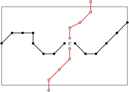
Figure 3.1: Primal and dual paths in the rectangle $R$. A black path is an open primal path joining an endpoint of $e$ to a left/right side of $R$, and a red path is an open dual path from an endpoint of $e_{\text{\rm d}}$ to the top/bottom side of $R$. An edge $e$ is pivotal for the box-crossing event if and only if there are four arms of alternating type from $e$ to the boundary of the box.

It turns out that the nature of the percolation singularity is partly determined by the asymptotic behaviour of the probability of such a ‘four-arm event’ at the critical point. This event has an associated critical exponent which we introduce next.

Let $\Lambda_{n}$ be the set of vertices within graph-theoretic distance $n$ of the origin $0$, with boundary $\partial\Lambda_{n}=\Lambda_{n}\setminus\Lambda_{n-1}$. Let $\mathcal{A}(N,n)=\Lambda_{n}\setminus\Lambda_{N-1}$ be the annulus centred at $0$. We call $\partial\Lambda_{n}$ (respectively, $\partial\Lambda_{N}$) its exterior (respectively, interior) boundary.

Let $k\in\mathbb{N}$, and let $\sigma=(\sigma_{1},\sigma_{2},\dots,\sigma_{k})\in\{0,1\}^{k}$; we call $\sigma$ a colour sequence. The sequence $\sigma$ is called monochromatic if either $\sigma=(0,0,\dots,0)$ or $\sigma=(1,1,\dots,1)$, and bichromatic otherwise. If $k$ is even, $\sigma$ is called alternating if either $\sigma=(0,1,0,1,\dots)$ or $\sigma=(1,0,1,0,\dots)$. An open path of the primal (respectively, dual) lattice is said to have colour 1 (respectively, 0). For $0<N<n$, the arm event $A_{\sigma}(N,n)$ is the event that the inner boundary of ${\mathcal{A}}(N,n)$ is connected to the outer boundary by $k$ vertex-disjoint paths with colours $\sigma_{1},\ldots,\sigma_{k}$, taken in anticlockwise order.

The choice of $N$ is largely immaterial to the asymptotics as $n\to\infty$, and it is enough to take $N=N(\sigma)$ sufficiently large that, for $n\geq N$, there exists a configuration with the required $j$ coloured paths. It is believed that there exist arm exponents $\rho(\sigma)$ satisfying

$$\mathbb{P}_{p_{\text{\rm c}}}[A_{\sigma}(N,n)]\approx n^{-\rho(\sigma)}\qquad\text{as }n\to\infty.$$

Of particular interest here are the alternating arm exponents. Let $j\in\mathbb{N}$, and write $\rho_{2j}=\rho(\sigma)$ with $\sigma$ the alternating colour sequence of length $2j$. Thus, $\rho_{4}$ is the exponent associated with the derivative of box-crossing probabilities. Note that the radial exponent $\rho$ satisfies $\rho=1/\rho(\{1\})$.

3.4 Star–triangle transformation

In its base form, the star–triangle transformation  is a simple graph-theoretic relation. Its principal use has been to explore models with characteristics that are invariant under such transformations. It was discovered in the context of electrical networks by Kennelly [36] in 1899, and it was adapted in 1944 by Onsager [52] to the Ising model in conjunction with Kramers–Wannier duality. It is a key element in the work of Baxter [3] on exactly solvable models in statistical mechanics, and it has become known as the Yang–Baxter equation (see [53] for a history of its importance in physics). Sykes and Essam [64] used the star–triangle transformation to predict the critical surfaces of inhomogeneous bond percolation on triangular and hexagonal lattices, and it is a tool in the study of the random-cluster model [21], and the dimer model [37].

Its importance for probability stems from the fact that a variety of probabilistic models are conserved under this transformation, including critical percolation, Potts, and random-cluster models. More specifically, the star–triangle transformation  provides couplings of critical probability measures under which certain geometrical properties of configurations (such as connectivity in percolation) are conserved.

Figure 3.2: The star–triangle transformation

We summarize the star–triangle transformation for percolation as in [20, Sect. 11.9]. Consider the triangle $G=(V,E)$ and the star $G^{\prime}=(V^{\prime},E^{\prime})$ drawn in Figure 3.2. Let $\mathbf{p}=(p_{0},p_{1},p_{2})\in[0,1)^{3}$. Write $\Omega=\{0,1\}^{E}$ with associated (inhomogeneous) product probability measure $\mathbb{P}_{\mathbf{p}}^{\triangle}$ with intensities $(p_{i})$ as illustrated, and $\Omega^{\prime}=\{0,1\}^{E^{\prime}}$ with associated measure $\mathbb{P}_{1-\mathbf{p}}^{\hexagon}$. Let $\omega\in\Omega$ and $\omega^{\prime}\in\Omega^{\prime}$. The configuration $\omega$ (respectively, $\omega^{\prime}$) induces a connectivity relation on the set $\{A,B,C\}$ within $G$ (respectively, $G^{\prime}$). It turns out that these two connectivity relations are equi-distributed so long as $\kappa_{\triangle}(\mathbf{p})=0$, where

$$\kappa_{\triangle}(\mathbf{p})=p_{0}+p_{1}+p_{2}-p_{1}p_{2}p_{3}-1.$$ (3.4)

This may be stated rigorously as follows. Let $1(x\xleftrightarrow{G,\omega}y)$ denote the indicator function of the event that $x$ and $y$ are connected in $G$ by an open path of $\omega$. Thus, connections in $G$ are described by the family $\{1(x\xleftrightarrow{G,\omega}y):x,y\in V\}$ of random variables, and similarly for $G^{\prime}$. It may be checked (or see [20, Sect. 11.9]) that the families

$$\left\{1(x\xleftrightarrow{G,\omega}y):x,y=A,B,C\right\},\quad\left\{1(x\xleftrightarrow{G^{\prime},\omega^{\prime}}y):x,y=A,B,C\right\},$$

have the same law whenever $\kappa_{\triangle}(\mathbf{p})=0$.

It is helpful to express this in terms of a coupling of $\mathbb{P}_{\mathbf{p}}^{\triangle}$ and $\mathbb{P}_{1-\mathbf{p}}^{\hexagon}$. Suppose $\mathbf{p}\in[0,1)^{3}$ satisfies $\kappa_{\triangle}(\mathbf{p})=0$, and let $\Omega$ (respectively, $\Omega^{\prime}$) have associated measure $\mathbb{P}_{\mathbf{p}}^{\triangle}$ (respectively, $\mathbb{P}_{1-\mathbf{p}}^{\hexagon}$) as above. There exist random mappings $T:\Omega\to\Omega^{\prime}$ and $S:\Omega^{\prime}\to\Omega$ such that:

• $T(\omega)$ has the same law as $\omega^{\prime}$, namely $\mathbb{P}_{1-\mathbf{p}}^{\hexagon}$,

• $S(\omega^{\prime})$ has the same law as $\omega$, namely $\mathbb{P}_{\mathbf{p}}^{\triangle}$,

• for $x,y\in\{A,B,C\}$, $1\bigl{(}x\xleftrightarrow{G,\omega}y\bigr{)}=1\bigl{(}x\xleftrightarrow{G^{\prime},T(\omega)}y\bigr{)}$,

• for $x,y\in\{A,B,C\}$, $1\bigl{(}x\xleftrightarrow{G^{\prime},\omega^{\prime}}y\bigr{)}=1\bigl{(}x\xleftrightarrow{G,S(\omega^{\prime})}y\bigr{)}$.

Such mappings are described informally in Figure 3.3 (taken from [23]).

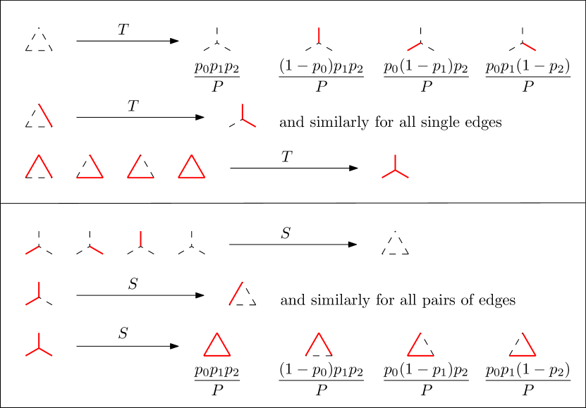
Figure 3.3: The random maps $T$ and $S$ and their transition probabilities, with $P:=(1-p_{0})\times$ $(1-p_{1})(1-p_{2})$. Note that $T(\omega)$ is deterministic for seven of the eight elements of $\Omega$; only in the eighth case does $T(\omega)$ involve further randomness. Similarly, $S(\omega^{\prime})$ is deterministic except for one special $\omega^{\prime}$.

The star–triangle transformation may evidently be used to couple bond percolation on the triangular and hexagonal lattices. This may be done, for example, by applying it to every upwards pointing triangle of $\mathbb{T}$. Its impact however extends much beyond this. Whenever two percolation models are related by sequences of disjoint star–triangle transformations, their open connections are also related (see [25]). That is, the star–triangle transformation transports not only measures but also open connections. We shall see how this may be used in the next section.

3.5 Universality for bond percolation

The hypothesis of universality states in the context of percolation that the nature of the singularity depends on the number of dimensions but not further on the details of the model (such as choice of lattice, and whether bond or site). In this section, we summarize results of [23, 24] showing a degree of universality for a class of bond percolation models in two dimensions. The basic idea is as follows. The star–triangle transformation is a relation between a large family of critical bond percolation models. Since it preserves open connections, these models have singularities of the same type.

We concentrate here on the square, triangular, and hexagonal (or honeycomb) lattices, denoted respectively as $\mathbb{L}^{2}$, $\mathbb{T}$, and $\mathbb{H}$. The following analysis applies to a large class of so-called isoradial graphs of which these lattices are examples (see [25]). The critical probabilities of homogeneous percolation on these lattices are known as follows (see [20]): $p_{\text{\rm c}}(\mathbb{L}^{2})=\frac{1}{2}$, and $p_{\text{\rm c}}(\mathbb{T})=1-p_{\text{\rm c}}(\mathbb{H})$ is the root in the interval $(0,1)$ of the cubic equation $3p-p^{3}-1=0$.

We define next inhomogeneous percolation on these lattices. The edges of the square lattice are partitioned into two classes (horizontal and vertical) of parallel edges, while those of the triangular and hexagonal lattices may be split into three such classes. The product measure on the edge-configurations is permitted to have different intensities on different edges, while requiring that any two parallel edges have the same intensity. Thus, inhomogeneous percolation on the square lattice has two parameters, $p_{0}$ for horizontal edges and $p_{1}$ for vertical edges, and we denote the corresponding measure $\mathbb{P}_{\mathbf{p}}^{\square}$ where $\mathbf{p}=(p_{0},p_{1})\in[0,1)^{2}$. On the triangular and hexagonal lattices, the measure is defined by a triplet of parameters $\mathbf{p}=(p_{0},p_{1},p_{2})\in[0,1)^{3}$, and we denote these measures $\mathbb{P}_{\mathbf{p}}^{\triangle}$ and $\mathbb{P}_{\mathbf{p}}^{\hexagon}$, respectively.

Criticality is identified in an inhomogeneous model via a ‘critical surface’. Consider bond percolation on a lattice ${\mathcal{L}}$ with edge-probabilities $\mathbf{p}=(p_{0},p_{1},\dots)$. The critical surface is an equation of the form $\kappa(\mathbf{p})=0$, where the percolation probability $\theta(\mathbf{p})$ satisfies

$$\theta(\mathbf{p})\begin{cases}=0&\text{if }\kappa(\mathbf{p})<0,\\ >0&\text{if }\kappa(\mathbf{p})>0.\end{cases}$$

The discussion of Section 3.2 may be adapted to the critical surface of an inhomogeneous model.

The critical surfaces of the above models are given explicitly in [20, 38]. Let

$$\kappa_{\square}(\mathbf{p}) =p_{0}+p_{1}-1, \quad\mathbf{p}=(p_{0},p_{1}),$$

$$\kappa_{\triangle}(\mathbf{p}) =p_{0}+p_{1}+p_{2}-p_{0}p_{1}p_{2}-1, \quad\mathbf{p}=(p_{0},p_{1},p_{2}),$$

$$\kappa_{\hexagon}(\mathbf{p}) =-\kappa_{\triangle}(1-p_{0},1-p_{1},1-p_{2}), \quad\mathbf{p}=(p_{0},p_{1},p_{2}).$$

The critical surface of the lattice $\mathbb{L}^{2}$ (respectively, $\mathbb{T}$, $\mathbb{H}$) is given by $\kappa_{\square}(\mathbf{p})=0$ (respectively, $\kappa_{\triangle}(\mathbf{p})=0$, $\kappa_{\hexagon}(\mathbf{p})=0$).

Let ${\mathcal{M}}$ denote the set of all inhomogeneous bond percolation models on the square, triangular, and hexagonal lattices, with edge-parameters belonging to the half-open interval $[0,1)$ and lying in the appropriate critical surface. A critical exponent $\pi$ is said to exist for a model $M\in{\mathcal{M}}$ if the appropriate asymptotic relation of Table 3.1 holds, and $\pi$ is called ${\mathcal{M}}$-invariant if it exists for all $M\in{\mathcal{M}}$ and its value is independent of the choice of such $M$.

Theorem 3.3 ([24]).

• For every $\pi\in\{\rho\}\cup\{\rho_{2j}:j\geq 1\}$, if $\pi$ exists for some model $M\in{\mathcal{M}}$, then it is ${\mathcal{M}}$-invariant.

• If either $\rho$ or $\eta$ exist for some $M\in{\mathcal{M}}$, then $\rho$, $\delta$, $\eta$ are ${\mathcal{M}}$-invariant and satisfy the scaling relations $2\rho=\delta+1$, $\eta\rho=2$.

Kesten [40] showed that the ‘near-critical’ exponents $\beta$, $\gamma$, $\nu$, $\Delta$ may be given explicitly in terms of $\rho$ and $\rho_{4}$, for two-dimensional models satisfying certain symmetries. Homogeneous percolation on our three lattices have these symmetries, but it is not known whether the strictly inhomogeneous models have sufficient regularity for the conclusions to apply. The next theorem is a corollary of Theorem 3.3 in the light of the results of [40, 51].

Theorem 3.4 ([24]).

Assume that $\rho$ and $\rho_{4}$ exist for some $M\in{\mathcal{M}}$. Then $\beta$, $\gamma$, $\nu$, and $\Delta$ exist for homogeneous percolation on the square, triangular and hexagonal lattices, and they are invariant across these three models. Furthermore, they satisfy the scaling relations $\gamma+2\beta=\beta(\delta+1)=2\nu$, $\Delta=\beta\delta$.

A key intermediate step in the proof of Theorem 3.3 is the box-crossing property for inhomogeneous percolation on these lattices.

Theorem 3.5 ([23]).

• If $\mathbf{p}\in(0,1)^{2}$ satisfies $\kappa_{\square}(\mathbf{p})=0$, then $\mathbb{P}_{\mathbf{p}}^{\square}$ has the box-crossing property.

• If $\mathbf{p}\in[0,1)^{3}$ satisfies $\kappa_{\triangle}(\mathbf{p})=0$, then both $\mathbb{P}_{\mathbf{p}}^{\triangle}$ and $\mathbb{P}_{1-\mathbf{p}}^{\hexagon}$ have the box-crossing property.

In the remainder of this section, we outline the proof of Theorem 3.5 and indicate the further steps necessary for Theorem 3.3. The starting point is the observation of Baxter and Enting [4] that the star–triangle transformation may be used to transform the square into the triangular lattice. Consider the ‘mixed lattice’ on the left of Figure 3.4 (taken from [23]), in which there is an interface $I$ separating the square from the triangular parts. Triangular edges have length $\sqrt{3}$ and vertical edges length $1$. We apply the star–triangle transformation to every upwards pointing triangle, and then to every downwards pointing star. The result is a translate of the mixed lattice with the interface lowered by one step. When performed in reverse, the interface is raised one step.

\psfrag{tu}{$T^{\vartriangle}$}\psfrag{td}{$T^{\triangledown}$}\psfrag{su}{$S^{\Yup}$}\psfrag{sd}{$S^{\Ydown}$}\includegraphics[width=433.62pt]{trans.eps}

Figure 3.4: Transformations $S^{\Yup}$, $S^{\Ydown}$, $T^{\vartriangle}$, and $T^{\triangledown}$ of mixed lattices. The transformations map the dashed stars/triangles to the bold stars/triangles. The interface-height decreases by $1$ from the leftmost to the rightmost graph.

This star–triangle map is augmented with probabilities as follows. Let $\mathbf{p}=(p_{0},p_{1},p_{2})\in[0,1)^{3}$ satisfy $\kappa_{\triangle}(\mathbf{p})=0$. An edge $e$ of the mixed lattice is declared open with probability:

• $p_{0}$ if $e$ is horizontal,

• $1-p_{0}$ if $e$ is vertical,

• $p_{1}$ if $e$ is the right edge of an upwards pointing triangle,

• $p_{2}$ if $e$ is the left edge of an upwards pointing triangle,

and the ensuing product measure is written $\mathbb{P}_{\mathbf{p}}$. Write $S^{\Ydown}\circ T^{\vartriangle}$ for the left-to-right map of Figure 3.4, and $S^{\Yup}\circ T^{\triangledown}$ for the right-to-left map. As described in Section 3.4, each $\tau\in\{S^{\Ydown}\circ T^{\vartriangle},S^{\Yup}\circ T^{\triangledown}\}$ may be extended to maps between configuration spaces, and they give rise to couplings of the relevant probability measures under which local open connections are preserved. It follows that, for a open path $\pi$ in the domain of $\tau$, the image $\tau(\pi)$ contains an open path $\pi^{\prime}$ with endpoints within distance 1 of those of $\pi$, and furthermore every point of $\pi^{\prime}$ is within distance $1$ of some point in $\pi$. We shall speak of $\pi$ being transformed to $\pi^{\prime}$ under $\tau$.

Let $\alpha>2$ and let $R_{N}$ be a $2\alpha N\times N$ rectangle in the square part of a mixed lattice. Since $\mathbb{P}_{\mathbf{p}}$ is a product measure, we may take as interface the set $\mathbb{Z}\times\{N\}$. Suppose there is an open path $\pi$ crossing $R_{N}$ horizontally. By making $N$ applications of $S^{\Ydown}\circ T^{\vartriangle}$, $\pi$ is transformed into an open path $\pi^{\prime}$ in the triangular part of the lattice. As above, $\pi^{\prime}$ is within distance $N$ of $\pi$, and its endpoints are within distance $N$ of those of $\pi$. As illustrated in Figure 3.5, $\pi^{\prime}$ contains a horizontal crossing of a $2(\alpha-1)\times 2N$ rectangle $R^{\prime}_{N}$ in the triangular lattice. It follows that

$$\mathbb{P}^{\triangle}_{\mathbf{p}}(C(R^{\prime}_{N}))\geq\mathbb{P}_{(p_{0},1-p_{0})}^{\square}(C(R_{N})),\qquad N\geq 1.$$

This is one of two inequalities that jointly imply that, if $\mathbb{P}_{(p_{0},1-p_{0})}^{\square}$ has the box-crossing property  then so does $\mathbb{P}_{\mathbf{p}}^{\triangle}$. The other such inequality is concerned with vertical crossings of rectangles. It is not so straightforward to derive, and makes use of a probabilistic estimate based on the randomization within the map $S^{\Ydown}\circ T^{\vartriangle}$ given in Figure 3.3.

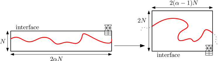
Figure 3.5: After $N$ applications of $S^{\Ydown}\circ T^{\vartriangle}$, a horizontal crossing of a rectangle of $\mathbb{Z}^{2}$ has been transformed into a crossing of a rectangle in $\mathbb{T}$ with altered aspect-ratio.

One may similarly show that $\mathbb{P}_{(p_{0},1-p_{0})}^{\square}$ has the box-crossing property whenever $\mathbb{P}_{\mathbf{p}}^{\triangle}$ has it. As above, two inequalities are needed, one of which is simple and the other less so. In summary, $\mathbb{P}_{(p_{0},1-p_{0})}^{\square}$ has the box-crossing property if and only if $\mathbb{P}_{\mathbf{p}}^{\triangle}$ has it. The reader is referred to [23] for the details.

Theorem 3.5 follows thus. It was shown by Russo [54] and by Seymour and Welsh [58] that $\mathbb{P}_{(\frac{1}{2},\frac{1}{2})}^{\square}$ has the box-crossing property (see also [22, Sect. 5.5]). By the above, so does $\mathbb{P}^{\triangle}_{\mathbf{p}}$ for $\mathbf{p}=(\frac{1}{2},p_{1},p_{2})$ whenever $\kappa_{\triangle}(\frac{1}{2},p_{1},p_{2})=0$. Similarly, so does $\mathbb{P}_{(p_{1},1-p_{1})}^{\square}$, and therefore also $\mathbb{P}_{\mathbf{p}}^{\triangle}$ for any triple $\mathbf{p}=(p_{0},p_{1},p_{2})$ satisfying $\kappa_{\triangle}(\mathbf{p})=0$.

\psfrag{tu}{$T^{-}$}\psfrag{td}{$T^{+}$}\psfrag{su}{$S^{+}$}\psfrag{sd}{$S^{-}$}\includegraphics[width=433.62pt]{strip.eps}

Figure 3.6: The transformation $S^{+}\circ T^{+}$ (respectively, $S^{-}\circ T^{-}$) transforms $\mathbb{L}^{1}$ into $\mathbb{L}^{2}$ (respectively, $\mathbb{L}^{2}$ into $\mathbb{L}^{1}$). They map the dashed graphs to the bold graphs.

We close this section with some notes on the further steps required for Theorem 3.3. We restrict ourselves to a consideration of the radial exponent $\rho$, and the reader is referred to [24] for the alternating-arm exponents. Rather than the mixed lattices of Figure 3.4, we consider the hybrid lattices $\mathbb{L}^{m}$ of Figure 3.6 having a band of square lattice of width $2m$, with triangular sections above and below. The edges of triangles have length $\sqrt{3}$ and the vertical edges length $1$. The edge-probabilities of $\mathbb{L}^{m}$ are as above, and the resulting measure is denoted $\mathbb{P}_{\mathbf{p}}^{m}$.

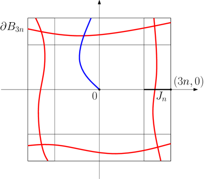
Figure 3.7: If $0$ is connected to $\partial B_{3n}$ and the four box-crossings occur, then $0$ is connected to the line-segment $J_{n}$.

Let $n\geq 3$, and $B_{n}=[-n,n]^{2}\subseteq\mathbb{R}^{2}$, and write $A_{n}=\{0\leftrightarrow\partial B_{n}\}$ where $\partial B$ denotes the boundary of the box $B$. Let $J_{n}$ be the line-segment $[2n,3n]\times\{0\}$, and note that $J_{n}$ is invariant under the lattice transformations of Figure 3.6. If $A_{3n}$ occurs, and in addition the four rectangles illustrated in Figure 3.7 have crossings, then $0\leftrightarrow J_{n}$. Let $\mathbf{p}\in[0,1)^{3}$. By Theorem 3.5 and positive association, there exists $\alpha>0$ such that, for $n\geq 3$,

$$\alpha\mathbb{P}^{\square}_{\mathbf{p}}(A_{3n}) \leq\mathbb{P}^{\square}_{\mathbf{p}}(0\leftrightarrow J_{n})\leq\mathbb{P}_{\mathbf{p}}^{\square}(A_{2n}),$$ (3.5)

$$\alpha\mathbb{P}^{\triangle}_{\mathbf{p}}(A_{3n}) \leq\mathbb{P}^{\triangle}_{\mathbf{p}}(0\leftrightarrow J_{n})\leq\mathbb{P}_{\mathbf{p}}^{\triangle}(A_{2n}).$$ (3.6)

By making $3n$ applications of the mapping $S^{+}\circ T^{+}$ (respectively, $S^{-}\circ T^{-}$) of Figure 3.6, we find that

$$\mathbb{P}_{(p_{0},1-p_{0})}^{\square}(0\leftrightarrow J_{n})=\mathbb{P}_{\mathbf{p}}^{3n}(0\leftrightarrow J_{n})=\mathbb{P}_{\mathbf{p}}^{0}(0\leftrightarrow J_{n})=\mathbb{P}_{\mathbf{p}}^{\triangle}(0\leftrightarrow J_{n}).$$

The equality of the exponents $\rho$ (if they exist) for these two models follows by (3.5)–(3.6), and the proof of Theorem 3.3(a) is completed in similar manner to that of the box-crossing property, Theorem 3.5.

Part (b) is a consequence of Theorem 3.5 on applying Kesten’s results of [39] about scaling relations at criticality.

4 Random-cluster model

4.1 Background

Let $G=(V,E)$ be a finite graph, and $\Omega=\{0,1\}^{E}$. For $\omega\in\Omega$, we write $\eta(\omega)=\{e\in E:\omega(e)=1\}$ for the set of open edges, and $k(\omega)$ for the number of connected components, or ‘open clusters’, of the subgraph $(V,\eta(\omega))$. The random-cluster measure on $\Omega$, with parameters $p\in[0,1]$, $q\in(0,\infty)$ is the probability measure

$$\phi_{p,q}(\omega)=\frac{1}{Z}\,\biggl{\{}\prod_{e\in E}p^{\omega(e)}(1-p)^{1-\omega(e)}\biggr{\}}q^{k(\omega)},\qquad\omega\in\Omega,$$ (4.1)

where $Z=Z_{G,p,q}$ is the normalizing constant. We assume throughout this section that $q\geq 1$, and for definiteness shall work only with the hypercubic lattice $\mathbb{L}^{d}=(\mathbb{Z}^{d},\mathbb{E}^{d})$ in $d\geq 2$ dimensions.

This measure was introduced by Fortuin and Kasteleyn in a series of papers around 1970, in a unification of electrical networks, percolation, Ising, and Potts models. Percolation is retrieved by setting $q=1$, and electrical networks arise via the limit $p,q\to 0$ in such a way that $q/p\to 0$. The relationship to Ising/Potts models is more complex in that it involves a transformation of measures. In brief, two-point connection probabilities for the random-cluster measure with $q\in\{2,3,\dots\}$ correspond to correlations for ferromagnetic Ising/Potts models, and this allows a geometrical interpretation of their correlation structure. A fuller account of the random-cluster model and its history and associations may be found in [21].

We omit an account of the properties of random-cluster measures, instead referring the reader to [21, 22]. Note however that random-cluster measures are positively associated whenever $q\geq 1$, in that (3.3) holds for all pairs $A$, $B$ of increasing events.

The random-cluster measure may not be defined directly on the hypercubic lattice $\mathbb{L}^{d}=(\mathbb{Z}^{d},\mathbb{E}^{d})$, since this is infinite. There are two possible ways to proceed, of which we choose here to use weak limits. Towards this end we introduce boundary conditions. Let $\Lambda$ be a finite box in $\mathbb{Z}^{d}$. For $b\in\{0,1\}$, define

$$\Omega_{\Lambda}^{b}=\{\omega\in\Omega:\omega(e)=b\text{ for }e\notin\mathbb{E}_{\Lambda}\},$$

where $\mathbb{E}_{\Lambda}$ is the set of edges of $\mathbb{L}^{d}$ joining pairs of vertices belonging to $\Lambda$. Each of the two values of $b$ corresponds to a certain ‘boundary condition’ on $\Lambda$, and we shall be interested in the effect of these boundary conditions in the infinite-volume limit.

On $\Omega_{\Lambda}^{b}$, we define a random-cluster measure $\phi_{\Lambda,p,q}^{b}$ as follows. Let

$$\phi_{\Lambda,p,q}^{b}(\omega)=\frac{1}{Z_{\Lambda,p,q}^{b}}\,\Biggl{\{}\prod_{e\in\mathbb{E}_{\Lambda}}p^{\omega(e)}(1-p)^{1-\omega(e)}\Biggr{\}}q^{k(\omega,\Lambda)},\qquad\omega\in\Omega_{\Lambda}^{b},$$ (4.2)

where $k(\omega,\Lambda)$ is the number of clusters of $(\mathbb{Z}^{d},\eta(\omega))$ that intersect $\Lambda$. The boundary condition $b=0$ (respectively, $b=1$) is sometimes termed ‘free’ (respectively, ‘wired’). The choice of boundary condition affects the measure through the total number $k(\omega,\Lambda)$ of open clusters: when using the wired boundary condition, the set of clusters intersecting the boundary of $\Lambda$ contributes only $1$ to this total.

The free/wired boundary conditions are extremal within a broader class. A boundary condition on $\Lambda$ amounts to a rule for how to count the clusters intersecting the boundary $\partial\Lambda$ of $\Lambda$. Let $\xi$ be an equivalence relation on $\partial\Lambda$; two vertices $v,w\in\partial\Lambda$ are identified as a single point if and only if $v\xi w$. Thus $\xi$ gives rise to a cluster-counting function $K(\cdot,\xi)$, and thence a probability measure $\phi_{\Lambda,p,q}^{\xi}$ as in (4.2). It is an exercise in Holley’s inequality [31] to show that

$$\phi_{\Lambda,p,q}^{\xi}\leq_{\text{\rm st}}\phi_{\Lambda,p,q}^{\xi^{\prime}}\qquad\text{if }\xi\leq\xi^{\prime},$$ (4.3)

where we write $\xi\leq\xi^{\prime}$ if, for all pairs $v$, $w$, $v\xi w\ \Rightarrow\ v\xi^{\prime}w$. In particular,

$$\phi_{\Lambda,p,q}^{0}\leq_{\text{\rm st}}\phi_{\Lambda,p,q}^{\xi}\leq_{\text{\rm st}}\phi_{\Lambda,p,q}^{1}\qquad\text{for all }\xi.$$ (4.4)

We may now take the infinite-volume limit. It may be shown that the weak limits

$$\phi_{p,q}^{b}=\lim_{\Lambda\to\mathbb{Z}^{d}}\phi_{\Lambda,p,q}^{b},\qquad b=0,1,$$

exist, and are translation-invariant and ergodic (see [19]). The limit measures, $\phi_{p,q}^{0}$ and $\phi_{p,q}^{1}$, are called ‘random-cluster measures’ on $\mathbb{L}^{d}$, and they are extremal in the following sense. There is a larger family of measures that can be constructed on $\Omega$, either by a process of weak limits, or by the procedure that gives rise to so-called DLR measures (see [21, Chap. 4]). It turns out that $\phi_{p,q}^{0}\leq_{\text{\rm st}}\phi_{p,q}\leq_{\text{\rm st}}\phi_{p,q}^{1}$ for any such measure $\phi_{p,q}$, as in (4.4). Therefore, there exists a unique random-cluster measure if and only if $\phi_{p,q}^{0}=\phi_{p,q}^{1}$.

The percolation probabilities are defined by

$$\theta^{b}(p,q)=\phi_{p,q}^{b}(0\leftrightarrow\infty),\qquad b=0,1,$$ (4.5)

and the critical values by

$$p_{\text{\rm c}}^{b}(q)=\sup\{p:\theta^{b}(p,q)=0\},\qquad b=0,1.$$ (4.6)

We are now ready to present a theorem that gives sufficient conditions under which $\phi_{p,q}^{0}=\phi_{p,q}^{1}$. The proof may be found in [21].

Theorem 4.1.

Let $d\geq 2$ and $q\geq 1$. We have that:

• [1] $\phi_{p,q}^{0}=\phi_{p,q}^{1}$ if $\theta^{1}(p,q)=0$,

• [19] there exists a countable subset ${\mathcal{D}}_{d,q}$ of $[0,1]$, possibly empty, such that $\phi_{p,q}^{0}=\phi_{p,q}^{1}$ if and only if $p\notin{\mathcal{D}}_{d,q}$.

By Theorem 4.1(b), $\theta^{0}(p,q)=\theta^{1}(p,q)$ for $p\notin{\mathcal{D}}_{d,q}$, whence $p_{\text{\rm c}}^{0}(q)=p_{\text{\rm c}}^{1}(q)$ by the monotonicity of the $\theta^{b}(\cdot,q)$. Henceforth we refer to the critical value as $p_{\text{\rm c}}(q)$. It is a basic fact that $p_{\text{\rm c}}(q)$ is non-trivial, which is to say that $0<p_{\text{\rm c}}(q)<1$ whenever $d\geq 2$ and $q\geq 1$.

It is an open problem to find a satisfactory definition of $p_{\text{\rm c}}(q)$ for $q<1$. Despite the failure of positive association in this case, it may be shown by the so-called ‘comparison inequalities’ (see [21, Sect. 3.4]) that there exists no infinite cluster for $q\in(0,1)$ and small $p$, whereas there is an infinite cluster for $q\in(0,1)$ and large $p$.

The following is an important conjecture ccncerning the discontinuity set ${\mathcal{D}}_{q}$.

Conjecture 4.2.

There exists $Q(d)$ such that:

• if $q<Q(d)$, then $\theta^{1}(p_{\text{\rm c}},q)=0$ and ${\mathcal{D}}_{d,q}=\varnothing$,

• if $q>Q(d)$, then $\theta^{1}(p_{\text{\rm c}},q)>0$ and ${\mathcal{D}}_{d,q}=\{p_{\text{\rm c}}\}$.

In the physical vernacular, there is conjectured to exist a critical value of $q$ beneath which the phase transition is continuous (‘second order’) and above which it is discontinuous (‘first order’). It was proved in [42, 44] that there is a first-order transition for large $q$, and it is expected that

$$Q(d)=\begin{cases}4&\text{if }d=2,\\ 2&\text{if }d\geq 6.\end{cases}$$

This may be contrasted with the best current rigorous estimate in two dimensions, namely $Q(2)\leq 25.72$, see [21, Sect. 6.4]. Recent progress towards a proof that $Q(2)=4$ is found in [8].

The third result of this article concerns the behaviour of the random-cluster model on the square lattice $\mathbb{L}^{2}$, and particularly its critical value.

4.2 Critical point on the square lattice

Theorem 4.3 ([7]).

The random-cluster model on $\mathbb{L}^{2}$ with cluster-weighting factor $q\geq 1$ has critical value

$$p_{\text{\rm c}}(q)=\frac{\sqrt{q}}{1+\sqrt{q}}.$$

This exact value has been ‘known’ for a long time, but the full proof has been completed only recently. When $q=1$, the statement $p_{\text{\rm c}}(1)=\frac{1}{2}$ is the Harris–Kesten theorem for bond percolation. When $q=2$, it amounts to the well known calculation of the critical temperature of the Ising model. For large $q$, the result was proved in [44, 45]. There is a ‘proof’ in the physics paper [30] when $q\geq 4$. It has been known since [19, 65] that $p_{\text{\rm sd}}(q)\geq\sqrt{q}/(1+\sqrt{q})$.

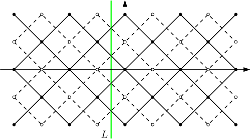
Figure 4.1: The lattice $\mathbb{L}^{2}$ and its dual, rotated through $\pi/4$. Under reflection in the green line $L$, the primal is mapped to the dual.

The main complication of Theorem 4.3 beyond the $q=1$ case stems from the interference of boundary conditions in the proof and applications of the box-crossing property, and this is where the major contributions of [7] are to be found. We summarize first the statement of the box-crossing property; the proof is outlined in Section 4.3. It is convenient to work on the square lattice $\mathbb{L}^{2}$ rotated through $\pi/4$, as illustrated in Figure 4.1. For $a=(a_{1},a_{2})\in\mathbb{N}^{2}$ and $b=(b_{1},b_{2})\in\mathbb{N}^{2}$, the rectangle $R_{a,b}$ of this graph is the subgraph induced by the vertices lying inside the rectangle $[a_{1},a_{2}]\times[b_{1},b_{2}]$ of $\mathbb{R}^{2}$. We shall consider two types of boundary condition on $R_{a,b}$. These affect the counts of clusters, and therefore the measures.

• all vertices in the boundary of a rectangle are identified as a single vertex.

• each vertex $(a_{1},y)$ (respectively, $(x,b_{1})$) of the boundary of $R_{a,b}$ is wired to $(a_{2},y)$ (respectively, $(x,b_{2})$).

Let $q\geq 1$, and write $p_{\text{\rm sd}}=\sqrt{q}/(1+\sqrt{q})$ and $B_{m}=R_{(-m,-m),(m,m)}$. The suffix in $p_{\text{\rm sd}}$ stands for ‘self-dual’, and its use is explained in the next section. The random-cluster measure on $B_{m}$ with parameters $p$, $q$ and boundary condition $b$ is denoted $\phi_{p,m}^{b}$. For a rectangle $R$, we write $C_{\text{\rm h}}(R)$ (respectively, $C_{\text{\rm v}}(R)$) for the event that $R$ is crossed horizontally (respectively, vertically) by an open path.

Proposition 4.4 ([7]).

There exists $c=c(q)>0$ such that, for $m>\frac{3}{2}n>0$,

$$\phi_{p_{\text{\rm sd}},m}^{\text{\rm per}}\left[C_{\text{\rm h}}\bigl{(}[0,\tfrac{3}{2}n)\times[0,n)\bigr{)}\right]\geq c.$$

The choice of periodic boundary condition is significant in that the ensuing measure is translation-invariant. Since the measure is invariant also under rotations through $\pi/2$, this inequality holds also for crossings of vertical boxes. Since random-cluster measures are positively associated, by Proposition 3.2, the measure $\phi_{p_{\text{\rm sd}},m}^{\text{\rm per}}$ satisfies a ‘finite-volume’ $\rho$-box-crossing property for all $\rho>1$.

An infinite-volume version of Proposition 4.4 will be useful later. Let $m>\frac{3}{2}n\geq 1$. By stochastic ordering (4.4),

$$\phi_{p_{\text{\rm sd}},m}^{1}\left[C_{\text{\rm h}}\bigl{(}[0,\tfrac{3}{2}n)\times[0,n)\bigr{)}\right] \geq\phi_{p_{\text{\rm sd}},m}^{\text{\rm per}}\left[C_{\text{\rm h}}\bigl{(}[0,\tfrac{3}{2}n)\times[0,n)\bigr{)}\right]$$

$$\geq c.$$ (4.7)

Let $m\to\infty$ to obtain

$$\phi_{p_{\text{\rm sd}},q}^{1}\left[C_{\text{\rm h}}\bigl{(}[0,\tfrac{3}{2}n)\times[0,n)\bigr{)}\right]\geq c,\qquad n\geq 1.$$ (4.8)

By Proposition 3.2, $\phi^{1}_{p_{\text{\rm sd}},q}$ has the box-crossing property. Equation (4.8) with $\phi_{p_{\text{\rm sd}},q}^{0}$ in place of $\phi_{p_{\text{\rm sd}},q}^{1}$ is false for large $q$, see [21, Thm 6.35].

Proposition 4.4 may be used to show also the exponential-decay of connection probabilities when $p<p_{\text{\rm sd}}$. See [7] for the details.

This section closes with a note about other two-dimensional models. The proof of Theorem 4.3 may be adapted (see [7]) to the triangular and hexagonal lattices, thus complementing known inequalities of [21, Thm 6.72] for the critical points. It is an open problem to prove the conjectured critical surfaces of inhomogeneous models on $\mathbb{L}^{2}$, $\mathbb{T}$, and $\mathbb{H}$. See [21, Sect. 6.6].

4.3 Proof of the box-crossing property

We outline the proof of Proposition 4.4, for which full details may be found in [7]. There are two steps: first, one uses duality to prove inequalities about crossings of certain regions; secondly, these are used to estimate the probabilities of crossings of rectangles.

Step 1, duality. Let $G=(V,E)$ be a finite, connected planar graph embedded in $\mathbb{R}^{2}$, and let $G_{\text{\rm d}}=(V_{\text{\rm d}},E_{\text{\rm d}})$ be its planar dual graph. A configuration $\omega\in\{0,1\}^{E}$ induces a configuration $\omega_{\text{\rm d}}\in\{0,1\}^{E_{\text{\rm d}}}$ as in Section 3.3 by $\omega(e)+\omega_{\text{\rm d}}(e_{\text{\rm d}})=1$.

We recall the use of duality for bond percolation on $\mathbb{L}^{2}$: there is a horizontal open primal crossing of the rectangle $[0,n+1]\times[0,n]$ (with the usual lattice orientation) if and only if there is no vertical open dual crossing of the dual rectangle. When $p=\frac{1}{2}$, both rectangle and probability measure are self-dual, and thus the chance of a primal crossing is $\frac{1}{2}$, whatever the value of $n$. See [20, Lemma 11.21].

Returning to the random-cluster measure on $G$, if $\omega$ has law $\phi_{G,p,q}$, it may be shown using Euler’s formula (see [21, Sect. 6.1] or [22, Sect. 8.5]) that $\omega_{\text{\rm d}}$ has law $\phi^{1}_{G_{\text{\rm d}},p_{\text{\rm d}},q}$ where

$$\frac{p}{1-p}\cdot\frac{p_{\text{\rm d}}}{1-p_{\text{\rm d}}}=q.$$

Note that $p=p_{\text{\rm d}}$ if and only if $p=p_{\text{\rm sd}}$. One must be careful with boundary conditions. If the primal measure has the free boundary condition, then the dual measure has the wired boundary condition (in effect, since $G_{\text{\rm d}}$ possesses a vertex in the infinite face of $G$).

Overlooking temporarily the issue of boundary condition, the dual graph of a rectangle $[0,n)^{2}$ in the square lattice is a rectangle in a shifted square lattice, and this leads to the aspiration to find a self-dual measure and a crossing event with probability bounded away from $0$ uniformly in $n$. The natural measure is $\phi_{p_{\text{\rm sd}},m}^{\text{\rm per}}$, and the natural event is $C_{\text{\rm h}}\bigl{(}[0,n)^{2}\bigr{)}$. Since this measure is defined on a torus, and tori are not planar, Euler’s formula cannot be applied directly. By a consideration of the homotopy of the torus, one obtains via an amended Euler formula that there exists $c_{1}=c_{1}(q)>0$ such that

$$\phi_{p_{\text{\rm sd}},m}^{\text{\rm per}}\left[C_{\text{\rm h}}\bigl{(}[0,n)^{2}\bigr{)}\right]\geq c_{1},\qquad 0<n<m.$$ (4.9)

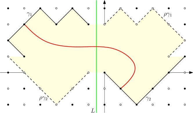
Figure 4.2: Under reflection $\rho$ in the green line $L$, the primal lattice is mapped to the dual. The primal path $\gamma_{1}$ is on the left side with an endpoint abutting $L$, and similarly $\gamma_{2}$ is on the right. Also, $\gamma_{1}$ and $\rho\gamma_{2}$ are non-intersecting with adjacent endpoints as marked.

We show next an inequality similar to (4.9) but for more general domains. Let $\gamma_{1}$, $\gamma_{2}$ be paths as described in the caption of Figure 4.2, and consider the random-cluster measure, denoted $\phi_{\gamma_{1},\gamma_{2}}$, on the primal graph within the coloured region $G(\gamma_{1},\gamma_{2})$ of the figure, with mixed wired/free boundary conditions obtained by identifying all points on $\gamma_{1}$, and similarly on $\gamma_{2}$ (these two sets are not wired together as one). For readers who prefer words to pictures: $\gamma_{1}$ (respectively, $\gamma_{2}$) is a path on the left (respectively, right) of the line $L$ of the figure, with exactly one endpoint adjacent to $L$; reflection in $L$ is denoted $\rho$; $\gamma_{1}$ and $\rho\gamma_{2}$ (and hence $\gamma_{2}$ and $\rho\gamma_{1}$ also) do not intersect, and their other endpoints are adjacent in the sense of the figure.

Writing $\{\gamma_{1}\leftrightarrow\gamma_{2}\}$ for the event that there is an open path in $G(\gamma_{1},\gamma_{2})$ from $\gamma_{1}$ to $\gamma_{2}$, we have by duality that

$$\phi_{\gamma_{1},\gamma_{2}}(\gamma_{1}\leftrightarrow\gamma_{2})+\phi^{*}_{\gamma_{1},\gamma_{2}}(\rho\gamma_{1}\leftrightarrow^{*}\rho\gamma_{2})=1,$$ (4.10)

where $\phi^{*}_{\gamma_{1},\gamma_{2}}$ is the random-cluster measure on the dual of the graph within $G(\gamma_{1},\gamma_{2})$ and $\leftrightarrow^{*}$ denotes the existence of an open dual connection. Now, $\phi^{*}_{\gamma_{1},\gamma_{2}}$ has a mixed boundary condition in which all vertices of $\rho\gamma_{1}\cup\rho\gamma_{2}$ are identified. Since the number of clusters with this wired boundary condition differs by at most 1 from that in which $\rho\gamma_{1}$ and $\rho\gamma_{2}$ are separately wired, the Radon–Nikodým derivative of $\phi^{*}_{\gamma_{1},\gamma_{2}}$ with respect to $\rho\phi_{\gamma_{1},\gamma_{2}}$ takes values in the interval $[q^{-1},q]$. Therefore,

$$\phi^{*}_{\gamma_{1},\gamma_{2}}(\rho\gamma_{1}\leftrightarrow^{*}\rho\gamma_{2})\leq{q^{2}}\phi_{\gamma_{1},\gamma_{2}}(\gamma_{1}\leftrightarrow\gamma_{2}).$$

By (4.10),

$$\phi_{\gamma_{1},\gamma_{2}}(\gamma_{1}\leftrightarrow\gamma_{2})\geq\frac{1}{1+q^{2}}.$$ (4.11)

Step 2, crossing rectangles. We show next how (4.11) may be used to prove Proposition 4.4. Let $S=S_{1}\cup S_{2}$, with $S_{1}=[0,n)\times[0,n)$ and $S_{2}=[\frac{1}{2}n,\frac{3}{2}n)\times[0,n)$, as illustrated in Figure 4.3. Let $A$ be the (increasing) event that: $S_{1}\cup S_{2}$ contains some open cluster $C$ that contains both a horizontal crossing of $S_{1}$ and a vertical crossing of $S_{2}$. We claim that

$$\phi^{\text{\rm per}}_{p_{\text{\rm sd}},m}(A)\geq\frac{c_{1}^{2}}{2(1+q^{2})},\qquad m\geq\tfrac{3}{2}n,$$ (4.12)

with $c_{1}$ as in (4.9). The proposition follows from (4.12) since, by positive association and (4.9),

$$\phi_{p_{\text{\rm sd}},m}^{\text{\rm per}}\left[C_{\text{\rm h}}\bigl{(}[0,\tfrac{3}{2}n)\times[0,n)\bigr{)}\right] \geq\phi^{\text{\rm per}}_{p_{\text{\rm sd}},m}\left[A\cap C_{\text{\rm h}}(S_{2})\right]$$

$$\geq\phi^{\text{\rm per}}_{p_{\text{\rm sd}},m}(A)\phi^{\text{\rm per}}_{p_{\text{\rm sd}},m}\left[C_{\text{\rm h}}(S_{2})\right]$$

$$\geq\frac{c_{1}^{3}}{2(1+q^{2})}.$$

We prove (4.12) next.

Let $\ell$ be the line-segment $[\frac{1}{2}n,n)\times\{0\}$, and let $C_{\text{\rm v}}^{\ell}(S_{2})$ be the event of a vertical crossing of $S_{2}$ whose only endpoint on the $x$-axis lies in $\ell$. By a symmetry of the random-cluster model, and (4.9),

$$\phi_{p_{\text{\rm sd}},m}^{\text{\rm per}}[C_{\text{\rm v}}^{\ell}(S_{2})]\geq\tfrac{1}{2}\phi^{\text{\rm per}}_{p_{\text{\rm sd}},q}[C_{\text{\rm v}}(S_{2})]\geq\tfrac{1}{2}c_{1}.$$ (4.13)

On the event $C_{\text{\rm h}}(S_{1})$ (respectively, $C_{\text{\rm v}}^{\ell}(S_{2})$) let $\Gamma_{1}$ (respectively, $\Gamma_{2}$) be the highest (respectively, rightmost) crossing of the required type. The paths $\Gamma_{i}$ may be used to construct the coloured region of Figure 4.3: $L$ is a line in whose reflection the primal and dual lattices are interchanged; the reflections $\rho\Gamma_{i}$ of the $\Gamma_{i}$ frame a region bounded by subsets $\gamma_{i}$ of $\Gamma_{i}$ and their reflections $\rho\gamma_{i}$. The situation is generally more complicated than the illustration in the figure since the $\Gamma_{i}$ can wander around $S$ (see [7]), but the essential ingredients of the proof are clearest thus.

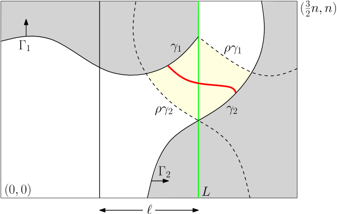
Figure 4.3: The path $\Gamma_{1}$ is the highest crossing of $S_{1}$, and $\Gamma_{2}$ is the rightmost crossing of $S_{2}$ starting in $\ell$. The coloured region is framed by the $\Gamma_{i}$ and their reflections in $L$. This is the simplest situation and there are more complex, depending on the $\Gamma_{i}$.

Let $I=\{\Gamma_{1}\cap\Gamma_{2}\neq\varnothing\}$, so that

$$\phi^{\text{\rm per}}_{p_{\text{\rm sd}},m}(A) \geq\phi^{\text{\rm per}}_{p_{\text{\rm sd}},m}\bigl{[}C_{\text{\rm h}}(S_{1})\cap C_{\text{\rm v}}^{\ell}(S_{2})\cap I\bigr{]}$$

$$\hskip 56.9055pt+\phi^{\text{\rm per}}_{p_{\text{\rm sd}},m}\bigl{[}A\cap C_{\text{\rm h}}(S_{1})\cap C_{\text{\rm v}}^{\ell}(S_{2})\cap I^{{\text{\rm c}}}\bigr{]}.$$ (4.14)

On the event $C_{\text{\rm h}}(S_{1})\cap C_{\text{\rm v}}^{\ell}(S_{2})\cap I^{{\text{\rm c}}}$,

$$\phi^{\text{\rm per}}_{p_{\text{\rm sd}},m}(A\mid\Gamma_{1},\Gamma_{2})\geq\phi^{\text{\rm per}}_{p_{\text{\rm sd}},m}\bigl{(}\gamma_{1}\leftrightarrow\gamma_{2}\text{ in }G(\gamma_{1},\gamma_{2})\,\big{|}\,\Gamma_{1},\Gamma_{2}\bigr{)}.$$

Since $\{\gamma\leftrightarrow\gamma_{2}\text{ in }G(\gamma_{1},\gamma_{2})\}$ is an increasing event, the right side is no larger if we augment the conditioning with the event that all edges of $S_{1}$ strictly above $\Gamma_{1}$ (and $S_{2}$ to the right of $\Gamma_{2}$) are closed. It may then be seen that

$$\phi^{\text{\rm per}}_{p_{\text{\rm sd}},m}\bigl{(}\gamma_{1}\leftrightarrow\gamma_{2}\text{ in }G(\gamma_{1},\gamma_{2})\,\big{|}\,\Gamma_{1},\Gamma_{2}\bigr{)}\geq\phi_{\gamma_{1},\gamma_{2}}(\gamma_{1}\leftrightarrow\gamma_{2}).$$ (4.15)

This follows from (4.3) by conditioning on the configuration off $G(\gamma_{1},\gamma_{2})$. By (4.13)–(4.14), (4.11), and positive association,

$$\phi^{\text{\rm per}}_{p_{\text{\rm sd}},m}(A) \geq\frac{1}{1+q^{2}}\phi^{\text{\rm per}}_{p_{\text{\rm sd}},m}\bigl{(}C_{\text{\rm h}}(S_{1})\cap C_{\text{\rm v}}^{\ell}(S_{2})\bigr{)}$$

$$\geq\frac{c_{1}^{2}}{2(1+q^{2})},$$

and (4.12) follows.

We repeat the need for care in deducing (4.15) in general, since the picture can be more complicated than indicated in Figure 4.3.

4.4 Proof of the critical value

The inequality $p_{\text{\rm c}}\geq p_{\text{\rm sd}}$ follows from the stronger statement $\theta^{0}(p_{\text{\rm sd}})=0$, and has been known since [19, 65]. Here is a brief explanation. We have that $\phi^{0}_{p,q}$ is ergodic and has the so-called finite-energy property. By the Burton–Keane uniqueness theorem [11], the number of infinite open clusters is either a.s. 0 or a.s. 1. If $\theta^{0}(p_{\text{\rm sd}})>0$, then a contradiction follows by duality, as in the case of percolation. Hence, $\theta^{0}(p_{\text{\rm sd}})=0$, and therefore $p_{\text{\rm c}}\geq p_{\text{\rm sd}}$. The details may be found in [21, Sect. 6.2].

It suffices then to show that $\theta^{1}(p)>0$ for $p>p_{\text{\rm sd}}$, since this implies $p_{\text{\rm c}}\leq p_{\text{\rm sd}}$. The argument of [7] follows the classic route for percolation, but with two significant twists. The first of these is the use of a sharp-threshold theorem for the random-cluster measure, combined with the uniform estimate of Proposition 4.4, to show that, when $p>p_{\text{\rm sd}}$, the chances of box-crossings are near to 1.

Proposition 4.5.

Let $p>p_{\text{\rm sd}}$. For integral $\beta>\alpha\geq 2$, there exist $a,b>0$ such that

$$\phi^{\text{\rm per}}_{p,\beta n}\left[C_{\text{\rm h}}\bigl{(}[0,\alpha n]\times[0,n)\bigr{)}\right]\geq 1-an^{-b},\qquad n\geq 1.$$

Outline proof.

Recall first the remark after Proposition 4.4 that $\phi^{\text{\rm per}}_{p_{\text{\rm sd}},m}$ has the $\alpha$-box-crossing property. Now some history. In proving that $p_{\text{\rm c}}=\frac{1}{2}$ for bond percolation on $\mathbb{L}^{2}$, Kesten used a geometrical argument to derive a sharp-threshold statement for box-crossings along the following lines: since crossings of rectangles with given aspect-ratio have probabilities bounded away from 0 when $p=\frac{1}{2}$, they have probability close to 1 when $p>\frac{1}{2}$. Kahn, Kalai, and Linial (KKL) [34] derived a general approach to sharp-thresholds of probabilities $\mathbb{P}_{\frac{1}{2}}(A)$ of increasing events $A$ under the product measure $\mathbb{P}_{\frac{1}{2}}$, and this was extended later to more general product measures (see [22, Chap. 4] and [35] for general accounts). Bollobás and Riordan [9] observed that the KKL method could be used instead of Kesten’s geometrical method. The KKL method works best for events and measures with a certain symmetry, and it is explained in [9] how this may be adapted for percolation box-crossings.

The KKL theorem was extended in [18] to measures satisfying the FKG lattice condition (such as, for example, random-cluster measures). The symmetrization argument of [9] may be adapted to the random-cluster model with periodic boundary condition (since the measure is translation-invariant), and the current proposition is a consequence.

See [7] for the details, and [22, Sect. 4.5] for an account of the KKL method, with proofs and references. ∎

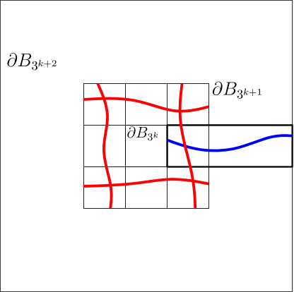
Figure 4.4: If the four red box-crossings exist, as well as the blue box-crossing, then the event $A_{k}$ occurs.

Let $p>p_{\text{\rm sd}}$, and consider the annulus ${\mathcal{A}}_{k}=B_{3^{k+1}}\setminus B_{3^{k}}$. Let $A_{k}$ be the event that ${\mathcal{A}}_{k}$ contains an open cycle $C$ with $0$ in its inside, and in addition there is an open path from $C$ to the boundary $\partial B_{3^{k+2}}$. We claim that there exist $c,d>0$, independent of $k$, such that

$$\phi^{1}_{p,3^{k+2}}(A_{k})\geq 1-ce^{-dk},\qquad k\geq 1.$$ (4.16)

This is proved as follows. The event $A_{k}$ occurs whenever the two rectangles

$$[-3^{k+1},-3^{k})\times[-3^{k+1},3^{k+1}],\quad(3^{k},3^{k+1}]\times[-3^{k+1},3^{k+1}]$$

are crossed vertically, and in addition the three rectangles

$$[-3^{k+1},3^{k+1}]\times[-3^{k+1},-3^{k}),\quad[-3^{k+1},3^{k+1}]\times(3^{k},3^{k+1}],$$

$$[3^{k},3^{k+2}]\times[-3^{k},3^{k}]$$

are crossed horizontally. See Figure 4.4. Each of these five rectangles has shorter dimension at least $3^{k}$ and longer dimension not exceeding $3^{k+2}$. By Proposition 4.5 and the invariance of $\phi^{\text{\rm per}}_{p,3^{k+2}}$ under rotations and translations, each of these five events has $\phi^{\text{\rm per}}_{p,3^{k+2}}$-probability at least $1-a3^{-bk}$ for suitable $a,b>0$. By stochastic ordering (4.3) and positive association,

$$\phi^{1}_{p,3^{k+2}}(A_{k})\geq\phi^{\text{\rm per}}_{p,3^{k+2}}(A_{k})\geq(1-a3^{-bk})^{5},$$

and (4.16) is proved.

Recall the weak limit $\phi_{p,q}^{1}=\lim_{k\to\infty}\phi^{1}_{p,3^{k}}$. The events $A_{k}$ have been defined in such a way that, on the event $I_{K}=\bigcap_{k=K}^{\infty}A_{k}$, there exists an infinite open cluster. It suffices then to show that $\phi_{p,q}^{1}(I_{K})>0$ for large $K$. Now,

$$\phi_{p,q}^{1}\left(\bigcap_{k=K}^{m}A_{k}\right)=\phi_{p,q}^{1}(A_{m})\prod_{k=K}^{m-1}\phi_{p,q}^{1}\left(A_{k}\,\left|\,\bigcap_{l=k+1}^{m}A_{l}\right.\right).$$ (4.17)

Let $\Gamma_{k}$ be the outermost open cycle in ${\mathcal{A}}_{k}$, whenever this exists. The conditioning on the right side of (4.17) amounts to the existence of $\Gamma_{k+1}$ together with the event $\{\Gamma_{k+1}\leftrightarrow\partial B_{3^{k+2}}\}$, in addition to some further information, $I$ say, about the configuration outside $\Gamma_{k+1}$. For any appropriate cycle $\gamma$, the event $\{\Gamma_{k+1}=\gamma\}\cap\{\gamma\leftrightarrow\partial B_{3^{k+2}}\}$ is defined in terms of the states of edges of $\gamma$ and outside $\gamma$. On this event, $A_{k}$ occurs if and only if $A_{k}(\gamma):=\{\Gamma_{k}\text{ exists}\}\cap\{\Gamma_{k}\leftrightarrow\gamma\}$ occurs. The latter event is measurable on the states of edges inside $\gamma$, and the appropriate conditional random-cluster measure is that with wired boundary condition inherited from $\gamma$, denoted $\phi^{1}_{\gamma}$. (We have used the fact that the cluster-count inside $\gamma$ is not changed by $I$.) Therefore, the term in the product on the right side of (4.17) equals the average over $\gamma$ of

$$\phi_{p,q}^{1}\left(A_{k}(\gamma)\,\Big{|}\,\{\Gamma_{k+1}=\gamma\}\cap\{\gamma\leftrightarrow\partial B_{3^{k+2}}\}\cap I\right)=\phi^{1}_{\gamma}(A_{k}(\gamma)).$$

Let $\Delta=\partial B_{3^{k+2}}$. Since $\phi_{\Delta}^{1}\leq_{\text{\rm st}}\phi^{1}_{\gamma}$ and $A_{k}(\Delta)\subseteq A_{k}(\gamma)$,

$$\phi^{1}_{\gamma}(A_{k}(\gamma))\geq\phi^{1}_{\Delta}(A_{k}(\Delta))=\phi^{1}_{p,3^{k+2}}(A_{k}).$$

In conclusion,

$$\phi_{p,q}^{1}\left(A_{k}\,\left|\,\bigcap_{l=k+1}^{m}A_{l}\right.\right)\geq\phi^{1}_{p,3^{k+2}}(A_{k}).$$ (4.18)

By (4.16)–(4.18),

$$\phi_{p,q}^{1}\left(\bigcap_{k=K}^{m}A_{k}\right)\geq\phi_{p,q}^{1}(A_{m})\prod_{k=K}^{m-1}(1-ce^{-dk}).$$

By (4.8), the box-crossing property, and positive association (as in the red paths of Figure 4.4), there exists $c_{2}>0$ such that $\phi_{p,q}^{1}(A_{m})\geq c_{2}$ for all $m\geq 1$. Hence,

$$\phi_{p,q}^{1}(I_{K})=\lim_{m\to\infty}\phi_{p,q}^{1}\left(\bigcap_{k=K}^{m}A_{k}\right)\geq c_{2}\prod_{k=K}^{\infty}(1-ce^{-dk}),$$

which is strictly positive for large $K$. Therefore $\theta^{1}(p,q)>0$, and the theorem is proved.

References

- [1] M. Aizenman, J. T. Chayes, L. Chayes, and C. M. Newman, Discontinuity of the magnetization in one-dimensional Ising and Potts models, J. Statist. Phys. 50 (1988), 1–40. MR 0939480
- [2] R. Bauerschmidt, H. Duminil-Copin, J. Goodman, and G. Slade, Lectures on self-avoiding-walks, Probability and Statistical Mechanics in Two and More Dimensions (D. Ellwood, C. M. Newman, V. Sidoravicius, and W. Werner, eds.), CMI/AMS publication, 2011.
- [3] R. J. Baxter, Exactly Solved Models in Statistical Mechanics, Academic Press, London, 1982. MR 0690578
- [4] R. J. Baxter and I. G. Enting, 399th solution of the Ising model, J. Phys. A: Math. Gen. 11 (1978), 2463–2473.
- [5] N. R. Beaton, J. de Gier, and A. G. Guttmann, The critical fugacity for surface adsorption of SAW on the honeycomb lattice is , Commun. Math. Phys., http://arxiv.org/abs/1109.0358.
- [6] V. Beffara, SLE and other conformally invariant objects, Probability and Statistical Mechanics in Two and More Dimensions (D. Ellwood, C. M. Newman, V. Sidoravicius, and W. Werner, eds.), CMI/AMS publication, 2011.
- [7] V. Beffara and H. Duminil-Copin, The self-dual point of the two-dimensional random-cluster model is critical for , Probab. Th. Rel. Fields, http://arxiv.org/abs/1006.5073.
- [8] V. Beffara, H. Duminil-Copin, and S. Smirnov, Parafermions in the random-cluster model, (2011).
- [9] B. Bollobás and O. Riordan, A short proof of the Harris–Kesten theorem, J. Lond. Math. Soc. 38 (2006), 470–484. MR 2239042
- [10] B. Bollobás and O. Riordan, Percolation, Cambridge University Press, Cambridge, 2006. MR 2283880
- [11] R. M. Burton and M. Keane, Density and uniqueness in percolation, Commun. Math. Phys. 121 (1989), 501–505. MR 0990777
- [12] F. Camia and C. M. Newman, Two-dimensional critical percolation, Commun. Math. Phys. 268 (2006), 1–38. MR 2249794
- [13] J. Cardy, Critical percolation in finite geometries, J. Phys. A: Math. Gen. 25 (1992), L201–L206. MR 1151081
- [14] D. Chelkak and S. Smirnov, Universality in the 2D Ising model and conformal invariance of fermionic observables, Invent. Math., http://arxiv.org/abs/0910.2045. MR 2275653
- [15] H. Duminil-Copin and S. Smirnov, The connective constant of the honeycomb lattice equals , Ann. Math., http://arxiv.org/abs/1007.0575.
- [16] B. Dyhr, M. Gilbert, T. Kennedy, G. F. Lawler, and S. Passon, The self-avoiding walk spanning a strip, J. Statist. Phys. 144 (2011), 1–22.
- [17] M. E. Fisher, On the dimer solution of planar Ising models, J. Math. Phys. 7 (1966), 1776–1781.
- [18] B. T. Graham and G. R. Grimmett, Influence and sharp-threshold theorems for monotonic measures, Ann. Probab. 34 (2006), 1726–1745. MR 2271479
- [19] G. R. Grimmett, The stochastic random-cluster process and the uniqueness of random-cluster measures, Ann. Probab. 23 (1995), 1461–1510. MR 1379156
- [20] G. R. Grimmett, Percolation, 2nd ed., Springer, Berlin, 1999. MR 1707339
- [21] G. R. Grimmett, The Random-Cluster Model, Springer, Berlin, 2006. MR 2243761
- [22] G. R. Grimmett, Probability on Graphs, Cambridge University Press, Cambridge, 2010, http://www.statslab.cam.ac.uk/~grg/books/pgs.html. MR 2723356
- [23] G. R. Grimmett and I. Manolescu, Inhomogeneous bond percolation on the square, triangular, and hexagonal lattices, Ann. Probab., http://arxiv.org/abs/1105.5535.
- [24] G. R. Grimmett and I. Manolescu, Universality for bond percolation in two dimensions, Ann. Probab., http://arxiv.org/abs/1108.2784.
- [25] G. R. Grimmett and I. Manolescu, Bond percolation on isoradial graphs, (2011), in preparation.
- [26] J. M. Hammersley and W. Morton, Poor man’s Monte Carlo, J. Roy. Statist. Soc. B 16 (1954), 23–38. MR 0064475
- [27] J. M. Hammersley and D. J. A. Welsh, Further results on the rate of convergence to the connective constant of the hypercubical lattice, Quart. J. Math. Oxford 13 (1962), 108–110. MR 0139535
- [28] T. Hara and G. Slade, Mean-field critical behaviour for percolation in high dimensions, Commun. Math. Phys. 128 (1990), 333–391. MR 1043524
- [29] T. Hara and G. Slade, Mean-field behaviour and the lace expansion, Probability and Phase Transition (G. R. Grimmett, ed.), Kluwer, 1994, pp. 87–122. MR 1283177
- [30] D. Hintermann, H. Kunz, and F. Y. Wu, Exact results for the Potts model in two dimensions, J. Statist. Phys. 19 (1978), 623–632. MR 0521142
- [31] R. Holley, Remarks on the FKG inequalities, Commun. Math. Phys. 36 (1974), 227–231. MR 0341552
- [32] B. D. Hughes, Random Walks and Random Environments; Volume I, Random Walks, Oxford University Press, Oxford, 1996.
- [33] I. Jensen and A. J. Guttman, Self-avoiding walks, neighbour-avoiding walks and trails on semiregular lattices, J. Phys. A: Math. Gen. 31 (1998), 8137–8145. MR 1651493
- [34] J. Kahn, G. Kalai, and N. Linial, The influence of variables on Boolean functions, Proceedings of 29th Symposium on the Foundations of Computer Science, 1988, pp. 68–80.
- [35] G. Kalai and S. Safra, Threshold phenomena and influence, Computational Complexity and Statistical Physics (A. G. Percus, G. Istrate, and C. Moore, eds.), Oxford University Press, New York, 2006, pp. 25–60. MR 2208732
- [36] A. E. Kennelly, The equivalence of triangles and three-pointed stars in conducting networks, Electrical World and Engineer 34 (1899), 413–414.
- [37] R. Kenyon, An introduction to the dimer model, School and Conference on Probability Theory, Lecture Notes Series, vol. 17, ICTP, Trieste, 2004, http://publications.ictp.it/lns/vol17/vol17toc.html, pp. 268–304. MR 2198850
- [38] H. Kesten, Percolation Theory for Mathematicians, Birkhäuser, Boston, 1982. MR 0692943
- [39] H. Kesten, A scaling relation at criticality for -percolation, Percolation Theory and Ergodic Theory of Infinite Particle Systems (H. Kesten, ed.), The IMA Volumes in Mathematics and its Applications, vol. 8, Springer, New York, 1987, pp. 203–212.
- [40] H. Kesten, Scaling relations for 2D-percolation, Commun. Math. Phys. 109 (1987), 109–156.
- [41] M. Klazar, On the theorem of Duminil-Copin and Smirnov about the number of self-avoiding walks in the hexagonal lattice, (2011), http://arxiv.org/abs/1102.5733.
- [42] R. Kotecký and S. Shlosman, First order phase transitions in large entropy lattice systems, Commun. Math. Phys. 83 (1982), 493–515. MR 0649814
- [43] G. Kozma and A. Nachmias, Arm exponents in high dimensional percolation, J. Amer. Math. Soc. 24 (2011), 375–409. MR 2748397
- [44] L. Laanait, A. Messager, S. Miracle-Solé, J. Ruiz, and S. Shlosman, Interfaces in the Potts model I: Pirogov–Sinai theory of the Fortuin–Kasteleyn representation, Commun. Math. Phys. 140 (1991), 81–91. MR 1124260
- [45] L. Laanait, A. Messager, and J. Ruiz, Phase coexistence and surface tensions for the Potts model, Commun. Math. Phys. 105 (1986), 527–545. MR 0852089
- [46] G. F. Lawler, Scaling limits and the Schramm–Loewner evolution, Probability Surveys 8 (2011).
- [47] G. F. Lawler, O. Schramm, and W. Werner, Conformal invariance of planar loop-erased random walks and uniform spanning trees, Ann. Probab. 32 (2004), 939–995. MR 2044671
- [48] G. F. Lawler, O. Schramm, and W. Werner, On the scaling limit of planar self-avoiding walk, Proc. Symposia Pure Math. 72 (2004), 339–365. MR 2112127
- [49] N. Madras and G. Slade, The Self-Avoiding Walk, Birkhäuser, Boston, 1993. MR 1197356
- [50] B. Nienhuis, Exact critical point and exponents of O models in two dimensions, Phys. Rev. Lett. 49 (1982), 1062–1065. MR 0675241
- [51] P. Nolin, Near-critical percolation in two dimensions, Electron. J. Probab. 13 (2008), 1562–1623. MR 2438816
- [52] L. Onsager, Crystal statistics. I. A two-dimensional model with an order–disorder transition, Phys. Rev. 65 (1944), 117–149. MR 0010315
- [53] J. H. H. Perk and H. Au-Yang, Yang–Baxter equation, Encyclopedia of Mathematical Physics (J.-P. Françoise, G. L. Naber, and S. T. Tsou, eds.), vol. 5, Elsevier, 2006, pp. 465–473.
- [54] L. Russo, A note on percolation, Z. Wahrsch’theorie verw. Geb. 43 (1978), 39–48. MR 0488383
- [55] O. Schramm, Scaling limits of loop-erased walks and uniform spanning trees, Israel J. Math. 118 (2000), 221–288. MR 1776084
- [56] O. Schramm, Conformally invariant scaling limits: an overview and collection of open problems, Proceedings of the International Congress of Mathematicians, Madrid (M. Sanz-Solé et al., ed.), vol. I, European Mathematical Society, Zurich, 2007, pp. 513–544.
- [57] O. Schramm and S. Sheffield, Contour lines of the two-dimensional discrete Gaussian free field, Acta Math. 202 (2009), 21–137. MR 2486487
- [58] P. D. Seymour and D. J. A. Welsh, Percolation probabilities on the square lattice, Ann. Discrete Math. 3 (1978), 227–245. MR 0494572
- [59] G. Slade, The self-avoiding walk: a brief survey, Surveys in Stochastic Processes (J. Blath, P. Imkeller, and S. Roelly, eds.), European Mathematical Society, 2010, Proceedings of the 33rd SPA Conference, Berlin, 2009.
- [60] S. Smirnov, Critical percolation in the plane: conformal invariance, Cardy’s formula, scaling limits, C. R. Acad. Sci. Paris Ser. I Math. 333 (2001), 239–244. MR 1851632
- [61] S. Smirnov, Towards conformal invariance of 2D lattice models, Proceedings of the International Congress of Mathematicians, Madrid, 2006 (M. Sanz-Solé et al., ed.), vol. II, European Mathematical Society, Zurich, 2007, pp. 1421–1452. MR 2275653
- [62] S. Smirnov and W. Werner, Critical exponents for two-dimensional percolation, Math. Res. Lett. 8 (2001), 729–744. MR 1879816
- [63] N. Sun, Conformally invariant scaling limits in planar critical percolation, Probability Surveys 8 (2011), 155–209.
- [64] M. F. Sykes and J. W. Essam, Some exact critical percolation probabilities for site and bond problems in two dimensions, J. Math. Phys. 5 (1964), 1117–1127. MR 0164680
- [65] D. J. A. Welsh, Percolation in the random-cluster process, J. Phys. A: Math. Gen. 26 (1993), 2471–2483. MR 1234408
- [66] W. Werner, Lectures on two-dimensional critical percolation, Statistical Mechanics (S. Sheffield and T. Spencer, eds.), vol. 16, IAS–Park City, 2007, pp. 297–360. MR 2523462
- [67] W. Werner, Percolation et Modèle d’Ising, Cours Specialisés, vol. 16, Société Mathématique de France, Paris, 2009.