Observing a column-dependent $\zeta$ in dense interstellar sources: the case of the Horsehead Nebula

Abstract

Context. Observations of small carbon-bearing molecules such as CCH, $\rm{C_{4}H}$, c–$\rm{C_{3}H_{2}}$, and HCO in the Horsehead Nebula have shown these species to have higher abundances towards the edge of the source than towards the center.

Aims. Given the determination of a wide range of values for $\zeta$ (s^-1), the total ionization rate of hydrogen atoms, and the proposal of a column-dependent $\zeta(N_{H})$, where $N_{H}$ is the total column of hydrogen nuclei, we desire to determine if the effects of $\zeta(N_{H})$ in a single object with spatial variation can be observable. We chose the Horsehead Nebula because of its geometry and high density.

Methods. We model the Horsehead Nebula as a near edge-on photon dominated region (PDR), using several choices for $\zeta$, both constant and as a function of column. The column-dependent $\zeta$ functions are determined by a Monte Carlo model of cosmic ray penetration, using a steep power-law spectrum and accounting for ionization and magnetic field effects. We consider a case with low-metal elemental abundances as well as a sulfur-rich case.

Results. We show that use of a column-dependent $\zeta(N_{H})$ of $5\times 10^{-15}$ s^-1 at the surface and $7.5\times 10^{-16}$ s^-1 at $A_{\rm V}=10$ on balance improves agreement between measured and theoretical molecular abundances, compared with constant values of $\zeta$.

Conclusions.

1 Introduction

Ion-neutral reactions are the most important driving processes for gas-phase chemistry. Therefore it is important to understand the mechanisms by which chemical species in the interstellar medium become ionized, in order to have a more accurate picture of the chemistry in various interstellar sources. Near the edge of dense clouds and throughout diffuse clouds, UV photons can provide a powerful ionizing force upon the medium, especially if there is a sufficiently strong source of radiation nearby. These photons do not penetrate very far into dense clouds, decreasing exponentially with the column density. Other ionizing agents, like X-rays, will penetrate farther into dense clouds, but deep within the object, high-energy ($\gtrsim 100$ MeV) cosmic rays are the dominant ionizing force.

The recent detection of unexpectedly large abundances of H${}_{3}^{+}$, however, in an assortment of diffuse clouds has raised the old question as to whether the high ionization rate needed is caused by a high flux of cosmic rays of $<1$ GeV (McCall et al., 2003; Indriolo et al., 2007). Such low energy cosmic rays would not be expected to penetrate deeply into dense clouds, so that a column-dependent ionization rate due to cosmic rays might exist in denser sources. This question is best explored by examining the influence of cosmic ray ionization at different depths into a single object, and the Horsehead Nebula is an ideal candidate for such an investigation.

The Horsehead Nebula, also called Barnard 33, is a dark nebula of size about $5^{\prime}$ in the bright nebula IC434. It is illuminated by $\rm{\sigma\leavevmode\nobreak\ Ori}$ from a distance of about $30^{\prime}$ (Anthony-Twarog, 1982). The radiation field incident on the cloud is most commonly taken to be $\chi=60$ in Draine units (Draine, 1978; Habart et al., 2005), and the geometry of the cloud is described as nearly “edge-on”, meaning that the line between $\rm{\sigma\leavevmode\nobreak\ Ori}$ and the Horsehead Nebula is nearly perpendicular to the line of sight. This makes the Horsehead Nebula ideal for observing column-dependent variables in a single source. It has an ambient magnetic field of $<6$ $\mu$G (Zaritsky et al., 1986) and a steep density gradient ranging from $10^{2}$ to $10^{5}$ cm^-3, and contains a pre-stellar core as well as at least one other dense region near the “throat” that will be able to be studied in greater detail by the Atacama Large Millimeter Array (ALMA) (Ward-Thompson et al., 2006).

High abundances of small carbon-bearing molecules were observed by Teyssier et al. (2004) and by Pety et al. (2005), with higher abundances of certain molecules ($\rm{CCH}$, c–$\rm{C_{3}H_{2}}$, $\rm{C_{4}H}$) observed near the edge than at the center. This led Pety et al. to posit that polycyclic aromatic hydrocarbons (PAH’s) near the edge of the cloud are being destroyed by incident radiation, and that the products of their destruction are these small hydrocarbons. A number of other molecules have been detected, including the ions HCO⁺ and HOC⁺ (Goicoechea et al., 2009b), the carbon-bearing neutrals $\rm{HCO}$ (Gerin et al., 2009), l–$\rm{C_{3}H}$, and c–$\rm{C_{3}H}$ (Teyssier et al., 2004), and the sulfur-bearing species $\rm{CS}$ and $\rm{HCS^{+}}$ (Goicoechea et al., 2006), although, except for HCO⁺, little information of their column dependence is available.

Chemical modeling of the Horsehead Nebula was discussed by Winnewisser & Herbst (1993). Teyssier et al. (2004) provided the first detailed chemical PDR model of the Horsehead Nebula, using the Meudon PDR code (Le Bourlot et al., 1993; Le Petit et al., 2002). A year later, Pety et al. (2005) modeled the Horsehead Nebula with the same code, comparing the results with observations at three different lines of sight, and incorporating PAH’s into the model. Habart et al. (2005) determined a column-dependent temperature via thermal balance. None of these models is able to account for the high abundances of small hydrocarbons at the edge, or the $\rm{HC_{3}N}$ abundance.

Deuterium fractionation of HCO⁺ ($[\rm{DCO^{+}}]/[\rm{HCO^{+}}]\sim 0.02$) has been observed in the Cloud region at $A_{\rm{V}}\approx 10$, and used to constrain its temperature to about $20$ K (Pety et al., 2007). Neutral atomic oxygen has also been detected (Goicoechea et al., 2009a), with hopes for Herschel’s heightened resolution to provide abundances of atomic oxygen for different regions in the cloud.

The effect of a higher sulfur abundance was considered by Goicoechea et al. (2006), using the Meudon code (Le Petit et al., 2006). Pety et al. (2007) also used this code to better understand deuterium fractionation at the Horsehead edge. The abundance of the negative ion $\rm{C_{6}H^{-}}$ was calculated by Millar et al. (2007), although negative ions have not yet been observed in this region. Morata & Herbst (2008) developed a time-dependent PDR code, and first applied it to the Horsehead Nebula, with mixed success. This is the code we make use of in this paper, in tandem with the Meudon PDR code, which we use to determine some of the physical conditions.

Compiègne et al. (2007) and Goicoechea et al. (2009b) have performed some recent modeling of the Horsehead region; Compiègne et al. (2007) explored the dust emission. Goicoechea et al. (2009b) self-consistently modeled the observed spatial distribution and line intensities with detailed depth-dependent predictions coupled with a nonlocal radiative transfer calculation for ${\rm H^{13}CO^{+}}$, ${\rm DCO^{+}}$ and ${\rm HOC^{+}}$. They compared their model results with the Gerin et al. (2009) observations of $\rm{HCO^{+}}$ in order to constrain the electron fraction. Goicoechea et al. determined a very steep relative electron abundance of $n_{e}/n_{H}\sim 10^{-4}-10^{-8}$ (where $n_{H}=n(\text{H})+2n(\rm{H_{2}})$) at $A_{\rm{V}}\approx 0.6-2.0$ from the cloud edge, based on a faint emission line attributed to $\rm{HCO^{+}}$ near the edge.

In this paper, we report our investigation on the effect of a column-dependent cosmic ray ionization rate $\zeta(N_{H})$ on model results for molecular abundances and their spatial variation in the Horsehead Nebula. This is offered as a partial explanation of the high abundances of small hydrocarbons at the edge of the Horsehead nebula. In Section 2, we discuss the determination of three different $\zeta(N_{H})$ functions, including a discussion of the role played by the magnetic field. In Section 3, we provide a detailed description of the PDR model used, and compare our calculated abundances with observational values using two different sets of elemental abundances. We also provide predicted abundances for observable species. In Section 4, we discuss the implications of these results, and a better determination of $\zeta(N_{H})$ from single sources after the advent of ALMA.

2 The Determination of $\zeta(N_{H})$

The cosmic ray ionization of the interstellar medium is caused primarily by relativistic protons, alpha particles, and electrons. This ionization rate, labeled $\zeta$, is typically represented as a per-second rate at which cosmic rays ionize atomic hydrogen. Given the process

$$\mathrm{H+CR\rightarrow H^{+}}+e^{-}+\mathrm{CR},$$

where CR represents ionizing cosmic rays, $\zeta$ is defined by the kinetic equation

$$\dfrac{d[\mathrm{H^{+}}]}{dt}=\zeta[\mathrm{H}],$$

where the brackets signify concentration. The ionization rate of other species, such as $\rm{H_{2}}$ and He, is usually determined in chemical networks by multiplying $\zeta$ by a constant. Even near the edge of dense clouds, the majority of hydrogen is molecular in nature, so it is important to note that, to a good approximation, $\zeta_{H2}\approx 2\zeta$ (Glassgold & Langer, 1974).

In the last decade, results from diffuse sources (McCall et al., 2003; Le Petit et al., 2004; Indriolo et al., 2007), including recent observations with Herschel (Gerin et al., 2010; Neufeld et al., 2010), have most often indicated that in these environments $\zeta$ is more than an order of magnitude higher than the generally accepted value of $10^{-17}$ s^-1. Earlier values for $\zeta$ ranging from $10^{-17}-10^{-15}$ s^-1 had been proposed (Spitzer & Tomasko, 1968; Hartquist et al., 1979; Dalgarno, 2006). Table 1 contains a limited historical overview of some of the values of $\zeta$ utilized in previous models. These actually refer to molecular rather than atomic hydrogen.

Table 1: Some values of $\zeta_{H2}$ used in previous models

$\zeta_{H2}$ ($\times 10^{-17}$ s-1)	Source
100	Solomon & Werner (1971)
1	Herbst & Klemperer (1973)
$3-2000$	Hartquist et al. (1978)
$10-100$	McCall et al. (2003)
25	Le Petit et al. (2004)
100	Goto et al. (2008)
$6-24$	Neufeld et al. (2010)
5000	Gupta et al. (2010)

The observations indicating a high $\zeta$, along with this wide range of values, led us to initiate a calculation of column-dependent functions of $\zeta$. At the same time, Padovani et al. (2009) undertook similar calculations. They used the ionization and energy loss cross sections for collisions between cosmic rays and atomic and molecular hydrogen (Cravens & Dalgarno, 1978) as well as Helium to follow the flux-spectra of cosmic rays through a cloud and, from the flux spectra as a function of position, obtained the column-dependent cosmic-ray ionization rate for a number of initial flux-spectra. Here we report similar calculations but with a Monte Carlo approach in which we also include magnetic field effects.

2.1 Initial Spectrum

We begin by considering the form of the initial cosmic ray flux-spectrum $j(E)$ (cm^-2 s^-1 sr^-1 GeV^-1 per nucleon), as a function of energy. The spectrum has only been directly observed within our solar system, where the solar wind would have depleted the low energy cosmic rays (Parker, 1958).

Different cosmic ray spectra have been proposed based on assumptions about the origin of the cosmic rays. Supernova shocks are currently the favored explanation for the origin of cosmic rays (Biermann et al., 2010; Axford, 1981). The spectrum due to the supernova blast alone imposes a low-energy cutoff at about $100\;\rm{MeV}$ because of energy loss due to debris and strong magnetic field effects (Hayakawa et al., 1961; Ip & Axford, 1985). It is suspected that shocks in the debris may re-accelerate some of the thermalized cosmic rays (Ip & Axford, 1985; Indriolo et al., 2009).

Shock models favor a steep power law for low-energy cosmic rays, with a new cutoff at 1 MeV, below which most cosmic rays would again lose a significant fraction of their energy into the debris, and would either be reabsorbed into the remnant, or would travel too slowly to propagate throughout the galaxy. Alternate theories for cosmic ray acceleration exist, but these also predict similar spectra for low-energy cosmic rays (Butt, 2009).

Comparison between measurements of the cosmic ray flux and theoretical cosmic ray spectra have been very useful. Basic statistics, “leaky-box” models, convection methods, and Monte Carlo methods have been applied to better constrain cosmic ray spectra, often by examining the elemental composition of the cosmic rays themselves. Strong et al. (2007) contains an excellent review of these methods. Webber (1998) incorporated the newest results from Voyager into their Monte Carlo model, in order to determine the low energy spectrum better.

Nevertheless, Voyager is still in a region where solar winds have a substantial effect. In fact, the farther the Voyager satellite travels, the steeper the low energy spectrum becomes (Webber, 1998). Indeed, as recently as Putze et al. (2011), statistical, Monte Carlo, and “leaky box” models have been unable to constrain the low energy cosmic ray spectrum, due to a lack of direct measurement of low energy cosmic ray protons outside the solar influence.

Indriolo et al. (2009) list many of the proposed cosmic ray spectra. We consider three representative spectra (Hayakawa et al., 1961; Spitzer & Tomasko, 1968; Nath & Biermann, 1994), which are shown in Figure 1. These three spectra span the range of low energy cosmic rays. The spectrum from Spitzer & Tomasko (1968) is based on solar system measurements of the low energy cosmic ray flux, and contains the minimum low-energy cosmic ray spectrum. Nath & Biermann (1994) assume that the power-law for the cosmic ray spectrum at $1$ GeV continues down until a hard cut-off at $1$ MeV. Theirs is the highest published estimate of the low energy cosmic ray flux. We chose to use these three spectra in order to provide the full range of impact that different low energy cosmic ray flux spectra have on the ionization rate. The spectrum of Nath & Biermann (1994) increases the most steeply towards lower energies, that of Spitzer & Tomasko (1968) actually decreases towards lower energies, and that of Hayakawa et al. (1961) lies in the middle.

2.2 Cross Sections

We calculate the loss of energy by considering $10^{4}$ cosmic ray protons with energies, $E$ (in eV unless otherwise noted), distributed according to the three spectra selected above. The particles stream into a cloud of a number density $n$ (cm^-3). At each distance increment, the particles are each assigned a random number, which is compared with the probability of an ionizing or other inelastic collision over an incremental distance, determined by cross-sections, $\sigma$ (cm²). For ionizing collisions by protons we use the form of $\sigma_{i}$ from Spitzer & Tomasko (1968). The cross section (cm²) for ionization of a hydrogen atom as a function of $E$ and the rest-energy of the proton ($E_{P}$) is given by

$$\sigma_{i,\text{H}}= 7.63\times 10^{-20}\left(1-\left(\frac{E_{P}}{E+E_{P}}\right)\right)^{-1}$$

$$+1.23\times 10^{-20}\log\left(\left(\frac{E+E_{P}}{E_{P}}\right)^{2}-1\right)$$

$$-5.29\times 10^{-21}.$$ (1)

The first term is dominant for “low” energies ($500$ keV $<E<50$ MeV), so for $E<50$ MeV, $\sigma_{i,\text{H}}\propto 1/E$, down to $E\approx 500$ keV, when Equation (1) ceases to be accurate. This cross-section is also used below for determining the cosmic ray ionization rate of atomic hydrogen. For molecular hydrogen, we simply multiply the cross section by a factor of 2.

Inelastic collisions are considered for atomic and molecular hydrogen only, and we use the cross-sections from Cravens et al. (1975), accounting for rotational, vibrational and electronic excitation as well as dissociation reactions. For the ionization of helium, the differential cross-section from Dalgarno et al. (1999) is integrated to yield a total cross section:

$$\sigma_{i,\text{He}}=1.5\epsilon_{0}A(E),$$ (2)

where $A(E)$ ($\propto 1/E$ for $E\lesssim 100$ MeV; $\propto\log(E)$ for $E\gtrsim 1$ GeV) and $\epsilon_{0}$ are parameters fit to the measurements of Shah et al. (1987).

2.3 Energy Loss

The energy loss calculation assumes a column great enough that the cosmic rays will collide with gaseous atoms and molecules many times. Since our model is one-dimensional, we do not consider the effects of elastic collisions on the exclusion of low energy cosmic rays from molecular clouds.

Because there are many collisions, we are justified in utilizing the average energy lost by cosmic ray in an ionizing collision, $\overline{W}$. This is equal to the ionization energy plus the average energy of the ejected electron. For molecular hydrogen, this is determined from the differential cross-section by Cravens & Dalgarno (1978); Dalgarno et al. (1999) to be

$$\overline{W}\;(\text{eV})=7.92E^{0.082}+4.76,$$ (3)

where $E$ (eV) is the energy of the cosmic ray before the ionizing event. The energy losses from other types of inelastic collisions with molecular hydrogen, as well as ionizing and other inelastic collisions with $\rm{H}$ and $\rm{He}$ are taken from the detailed forms in Cravens et al. (1975).

This energy loss is subtracted from the initial energy of the cosmic ray, and becomes the new energy. At each increment, a new flux-spectrum, $j(E,N_{H})$, is calculated, and new random numbers are assigned to the cosmic rays. Because of the energy-dependence of the $\sigma$ functions, lower energy cosmic rays have more ionizing collisions. In the case of the spectrum of Nath & Biermann (1994), cosmic rays with $E<50$ MeV contribute $99\%$ to the value of $\zeta$ (see Section 2.5). To complicate matters, however, there is energy loss from magnetic effects in addition to the loss from collisions. Magnetic energy loss is assigned based on interactions with Alfvén waves, as discussed below, using a static magnetic field of 3 $\mu$Gauss.

2.4 Magnetic Field Effects

Magnetic fields play an important role in the transport of cosmic rays. The Lorentz force is the largest magnetic force acting on cosmic rays, and affects energy loss by increasing the path length cosmic rays travel, as they spiral along the magnetic field lines. This resulting increase in path length is not, however, the primary source of energy loss. Rather, the dominant magnetic field effect on cosmic rays is due to irregularities in the magnetic field.

Because of the neutralization of low-energy cosmic rays, there will be far fewer cosmic rays at the center of the cloud than at the edge. Since cosmic rays are overwhelmingly positively charged, these losses introduce a charge imbalance in the cloud. Electrons are attracted to the edge, and their motion generates magnetic field irregularities moving from the center to the edge of the cloud with velocity $\upsilon_{A}=B(4\pi\rho)^{-1/2}$. These irregularities, called Alfvén waves, are the dominant source of energy loss, as discussed in Skilling & Strong (1976). Hartquist et al. (1978, 1979) first applied the work of Skilling & Strong (1976) to calculate cosmic ray ionization rates, and proposed different values of $\zeta$, depending on the object.

Following Skilling & Strong (1976), we determine the charge imbalance using the Monte Carlo simulation with $B=0$, and consider it in terms of a characteristic column density, $\lambda(E)$ (cm^-2), determined by the simulation, at which the number of cosmic rays will be depleted by a factor of $e$. This means that $N_{H}$ must be $\gtrsim\lambda(E)$ for cosmic rays of energy $E$ to be significantly affected by magnetic field irregularities. This function will appear later in the analysis.

Alfvén waves are driven by the charge imbalance, and are damped by the friction between ions and the surrounding gas, as discussed by McIvor (1975) in terms of the collision rate $\Gamma$ (s^-1) between ions and neutrals (Dalgarno & Dickinson, 1968). The larger $\Gamma$ is, the less effect the waves have. The static magnetic field enhances the damping by absorbing smaller irregularities. However, the larger static magnetic field also increases $\upsilon_{A}$, and thus the frequency of collisions between the cosmic rays and the Alfvén waves.

This mechanism for cosmic ray energy loss by Alfvén wave effects is important for $N_{H}<10^{24}$ cm^-2 when $B\lesssim 6$ mG and $n_{H}\lesssim 10^{9}$ cm^-3. At a given column density, cosmic ray energy is substantially affected by Alfvén waves for energies less than the energy $E_{0}$. The static magnetic field outside denser regions is assumed to be much smaller than the field inside these regions. Because the difference between the magnetic field inside and outside the cloud significantly dampens the Alfvén waves for mid to high energy cosmic rays, $E_{0}$ cannot be greater than $50$ MeV (Cesarsky & Volk, 1978). $E_{0}$ is dependent on various physical parameters of the source in question. For typical cold and dense interstellar conditions, $n(\rm{HI})=1$ cm^-3, $n_{H}=10^{4}$ cm^-3, $T=20$ K, and $B=3\;\mu$G. Under these conditions, the use of $j_{0}(E)$ from Nath & Biermann (1994) leads to $E_{0}=1$ MeV at $N_{H}=10^{19}$ cm^-2 , while for $N_{H}>10^{21}$ cm^-2, $E_{0}=50$ MeV.

Integrating over energies up to this cutoff value, we can obtain the magnetohydrodynamic solution for $j_{\rm{IC}}(E,N_{H})$, the “In-Cloud” cosmic ray flux-spectrum at a given $N_{H}$, to be (Skilling & Strong, 1976)

$$j_{\rm{IC}}(E<E_{0},N_{H})= \dfrac{\lambda(E)}{E}\Bigg{[}\dfrac{E_{0}j(E_{0},N_{H})}{\lambda(E_{0})}$$

$$+\dfrac{2\upsilon_{A}}{N_{H}}\int_{E^{\prime}=E}^{E_{0}}\dfrac{\alpha j(E^{\prime},N_{H})}{\upsilon(E^{\prime})}dE^{\prime}$$

$$+\dfrac{U_{M}\Gamma}{\pi^{2}m\upsilon_{A}\Omega_{0}N_{H}}\ln\Bigg{(}\dfrac{\gamma_{0}^{2}-1}{\gamma^{2}-1}\Bigg{)}\Bigg{]};$$ (4)

$$j_{\rm{IC}}(E>E_{0},N_{H})= j(E,N_{H})$$ (5)

In this expression, $j(E,N_{H})$ is the spectrum determined using the Monte Carlo simulation in the absence of magnetic field effects, the magnetic energy density $U_{M}=B^{2}/2\mu_{0}$ (erg/cm^-3), $\Omega_{0}$ is the gyromagnetic frequency (s^-1), the Compton-Getting factor $\alpha$ (Gleeson & Axford, 1968) is

$$\alpha=-\dfrac{10}{9}\dfrac{E}{j_{0}(E)}\dfrac{\partial j_{0}}{\partial E},$$

where $j_{0}$ is the initial cosmic ray flux-spectrum, $\gamma=(1-\upsilon^{2}/c^{2})^{-1/2}$ and $\gamma_{0}=(1-\upsilon_{0}^{2}/c^{2})^{-1/2}$ where $\upsilon_{0}$ is the velocity of a cosmic ray of energy $E_{0}$.

Given a steep initial $j_{0}(E)$, the approximate effect of the Alfvén waves and Lorentz Force is to shift the cosmic ray spectrum, and thus the ionization rate (see next section), from $\zeta(N_{H})$ to $\zeta(5N_{H})$, so that the ionization rate decreases more strongly with column.

For cosmic ray flux-spectra that are not very steep ($m<2$ for $j\propto E^{-m}$), the shift is less extreme. Of course, for the full description of the relationship of $\zeta$ to the column density, Equation (5) must be calculated for $E<E_{0}$.

2.5 The Column-Dependent Ionization Rate

The value of $\zeta(N_{H})$ is calculated by integrating the product of the flux-spectrum from eq. (5), $j_{\rm{IC}}(E,N_{H})$, and $\sigma_{i,\text{H}}(E)$ from eq. (1), as a function of “depth” $N_{H}$ into a cloud, with various correction factors:

$$\zeta(N_{H})=1.8\times\frac{5}{3}\times\int_{0}^{\infty}4\pi\sigma_{i,\text{H}}(E)j_{\rm IC}(E,N_{H})dE.$$ (6)

The factor of $5/3$ (Spitzer & Tomasko, 1968; Dalgarno et al., 1999) takes into account the additional ionization caused by secondary electrons, while the factor of 1.8 accounts for ionization due to $\alpha$ particles ($\rm{He^{+2}}$). These particles are the second most important source of ionizing cosmic rays ($\zeta_{\alpha}\approx 0.8\zeta_{p}$). By comparison, relativistic electrons, the third most important ionizing source, have little effect: $\zeta_{e}\sim\zeta_{p}/100$.

Three different functions for $\zeta(N_{H})$ have been calculated, based on the cosmic ray flux-spectra in Figure 1, which are chosen to be widely divergent below $E\approx 500$ MeV to account for the uncertainty in the low-energy region (Hayakawa et al., 1961; Spitzer & Tomasko, 1968; Nath & Biermann, 1994). Analytical expressions for $\zeta(N_{H})$, used in the models below, are:

$$\zeta_{H,\text{Hayakawa}} =\dfrac{5\times 10^{4}}{N_{H}}+10^{-17}\;\text{s${}^{-1}$},$$ (7)

$$\zeta_{H,\text{Nath}} =0.002(N_{H})^{-0.6}+10^{-17}\;\text{s${}^{-1}$},$$ (8)

and are valid for $10^{24}$ cm^-2 $\gtrsim N_{H}\gtrapprox 5\times 10^{19}$ cm^-2. These analytical expressions do not seem to change significantly for $100$ cm^-3 $<n<10^{6}$ cm^-3 and $5$ K $<T<1000$ K, beyond which the effects of the density and temperature on magnetic field effects becomes significant.

The results are depicted in Figure 2, in terms of the visual extinction between the cloud and the UV source ($A_{\rm V}$). We determine $A_{\rm V}\approx 4.3\times 10^{-22}N_{H}$, using $Q$ efficiencies from Laor & Draine (1993) with a grain distribution (in terms of the “radius” of the grain, $a$) of $n\propto a^{-3.5}$ with $r_{\rm min}=5$ nm and $r_{\rm max}=1$ $\mu$m. With these assumptions, the analytical expressions for $\zeta(A_{\rm V})$ are:

$$\zeta_{H,\text{Hayakawa}} =\dfrac{2.2\times 10^{-17}}{A_{\rm V}}+10^{-17}\;\text{s${}^{-1}$},$$ (9)

$$\zeta_{H,\text{Nath}} =3.05\times 10^{-16}(A_{\rm V})^{-0.6}+10^{-17}\;\text{s${}^{-1}$}.$$ (10)

These expressions are later referred to as “mid-range” and ’“high-range” values, respectively.

The wide range of the ionization rate demonstrates the importance of low-energy cosmic rays, especially at low $N_{H}$ or $A_{\rm V}$. Other calculations of $\zeta(N_{H})$ have been performed, either for high column densities ($>10^{24}$ cm^-2) where low energy cosmic rays do not penetrate (Umebayashi & Nakano, 1981; Finocchi & Gail, 1997), without consideration of the magnetic field (Padovani et al., 2009), or in regions where there are no ionization losses (Padoan & Scalo, 2005). Recently, Padovani & Galli (2011) have incorporated the effect of magnetic mirroring, whereas we have treated the effects of Alfvén waves on cosmic ray streaming. The results in this paper suggest that Alfvén waves may have a more substantial effect on $\zeta$, with factor of $\sim$10 impact on $\zeta$ at certain $N_{H}$ for Alfvén waves versus a factor of $\sim$2-4 impact on $\zeta$ from magnetic mirroring. Ultimately, a robust magnetohydrodynamics simulation of cosmic ray transport would be necessary to determine what magnetic field effects have the most significant impact on cosmic ray penetration.

In our study below, we determine the effect of four different functions for $\zeta$ on the chemistry in the Horsehead Nebula. We consider the $\zeta(N_{H})$ functions based on flux spectra from Nath & Biermann (1994) and Hayakawa et al. (1961), as well as constant values for $\zeta$ of $10^{-15}$ s^-1, and $10^{-17}$ s^-1, the latter of which is effectively the $\zeta(N_{H})$ derived from the spectrum of Spitzer & Tomasko (1968).

Figure 1: Three different cosmic ray flux spectra, taken from Hayakawa et al. (1961) (dashed line), Spitzer & Tomasko (1968) (dotted line), and Nath & Biermann (1994) (solid line).

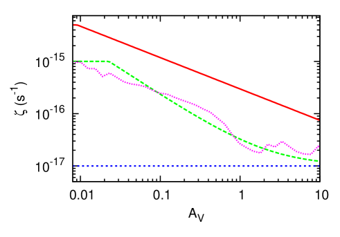
Figure 2: The results of the one-dimensional Monte Carlo model for $\zeta$ described in Section 2 in terms of $A_{\rm{V}}$. The solid red, dashed green, and dotted blue lines derive from the flux-spectra of Nath & Biermann (1994), Hayakawa et al. (1961), and Spitzer & Tomasko (1968), respectively. These lines fit the averaged result of dozens of iterations of the Monte Carlo model. The results from a single Monte Carlo run using the flux-spectrum of Hayakawa et al. (1961) are included (pink dotted) in order to show error.

3 Modeling the Horsehead Nebula

We have used the PDR model of Morata & Herbst (2008) with the OSU 03/2008 gas-phase network. This network is a purely gas-phase one that treats the PDR as a semi-infinite series of slabs with the radiation source impinging on one edge. It does not account for freeze-out or any surface chemistry, aside from a simple approximation for H₂ formation on grains and selected ion recombination processes. Radiative transfer and self-shielding of $\rm{H_{2}}$ and $\rm{CO}$ (Draine & Bertoldi, 1996; Lee et al., 1996b) are calculated in progression, starting with the slab at the edge. The chemistry is solved with a time-dependent gas-phase kinetics model for each slab. This model, like our model for cosmic rays, is one-dimensional (1D). Because cosmic rays are thought to stream in from all sides, the effects of the geometry are mostly lost in this model. However, even with cosmic rays streaming in from all angles, low energy cosmic rays will dominate at the edge, and will be absent from the center. The average value of $\zeta$ at a slab near the edge will be close to the value determined from the 1D Monte Carlo model. Because the majority of slabs near the center will not have low-energy cosmic rays, the average $\zeta$ near the center also be close to the 1D value. Thus the average value of $\zeta$ at different slabs of the cloud will be close to the 1D values we use for $\zeta$ found in Figure 2.

Following Pety et al. (2005), we compare, when possible, observations with model results for three regions at different optical extinctions ($A_{\rm{V}}$) from the edge of the Horsehead PDR. These are the IR-edge ($A_{\rm{V}}=1.56\pm 0.73$), IR-Peak ($A_{\rm{V}}=4.55\pm 1.7$), and the Cloud ($A_{\rm{V}}=11.7\pm 4.1$). The error bars in $A_{\rm V}$ are based both on the beam size of the observations and uncertainty in the density profile of the cloud, as discussed in the next section. We determine the error in fractional abundance by taking the ratio between the observed column density of the species and the error in that column density, both from Pety et al. (2005).

3.1 Physical Conditions and Initial Chemical Abundances

The density profiles used are taken from Habart et al. (2005). The temperature profile is calculated from thermal balance (Le Petit et al., 2006). Cosmic rays heat the interstellar medium through the thermalization of secondary electrons and photons, (Field et al., 1969; Glassgold & Langer, 1973). Thermal heating by cosmic rays begins to dominate at $A_{\rm{V}}>3$, but the thermal impact of different cosmic ray ionization rates is not very significant until $\zeta>10^{-16}$ s^-1. Since even the highest $\zeta(N_{H})$ drops to $\approx 10^{-16}$ s^-1 at the Cloud region, the temperature difference here between the high $\zeta(N_{H})$ and $\zeta=10^{-17}$ s^-1 is only about 4 K. The density and temperature profiles are shown in Fig. 3.

The gas density increases with spatial distance into the nebula as a power law with an exponent $\beta$ (Habart et al., 2005), which in terms of column density can be written as:

$$n_{H}(N_{H})=\begin{cases}n_{H,0}\Bigg{[}\dfrac{(\beta+1)N_{H}}{x_{0}n_{H,0}}\Bigg{]}^{\beta/(\beta+1)}&N_{H}\leq N_{H,0}\\ n_{H,0}&N_{H}>N_{H,0},\end{cases}$$ (11)

where $\beta\geq 1$ is a dimensionless constant used to parameterize the steepness of the number density, $n_{H,0}=2\times 10^{5}$ cm^-3, $x_{0}=0.02$ pc is a length scale, and $N_{H,0}=(1+\beta)^{-1}1.23\times 10^{22}$ cm^-2 is the column density at a depth of $x_{0}$. For our analysis, we show the results for $\beta=1$, and discuss results for both $\beta=1$ and $\beta=4$. The steeper density gradient impacts the UV photon flux and the resulting thermal balance. There are different total densities for the IR-edge and IR-peak regions. The difference in UV penetration, temperature and density at different values of $A_{\rm V}$ noticeably impacts the chemistry. The cosmic ray ionization, however, is not significantly altered by the density gradient, because for the ranges of density of $100$ to $10^{5}$ cm^-3, $\zeta$ is column-dependent, but not density dependent.

Other densities and density profiles have been proposed. Pety et al. (2005) used several uniform number densities and profiles, while Goicoechea et al. (2009b) proposed a slowly changing piecewise function for the density, with three sections instead of two, reaching $2\times 10^{5}$ cm^-3 at $A_{\rm{V}}\approx 5$ instead of $A_{\rm{V}}\approx 1.0$, as used here. Until the number density is better determined, significant uncertainties in the extinction at a given angular depth will persist.

Figure 3: The temperature (dashed line) and density (solid line) profiles as functions of visual extinction with $\zeta_{H,\text{\rm Nath}}$. The density profile is in the form of Habart et al. (2005), our equation (11), with $\beta=1$. The temperature is from thermal balance (Le Petit et al., 2006). At $A_{\rm V}=10$, $\zeta\approx 10^{-16}$ s^-1, which raises the temperature by $\approx 4$ K at the center compared to a $\zeta$ of $10^{-17}$ s^-1.

The UV radiation field impinging on the Horsehead surface has been a topic of much discussion and uncertainty (Anthony-Twarog, 1982; Zhou et al., 1993; Abergel et al., 2003). Values of $\chi=30$ to $\chi=100$ in Draine units (Draine, 1978) have been proposed. We use $\chi=60$, because this is the most commonly used value for the Horsehead PDR. The external UV field is important to the chemistry only for the IR-edge. For the IR-peak and the Cloud regions, cosmic rays are the primary ionizing and photochemical agent.

The initial chemical abundances used for the Horsehead PDR (Lee et al., 1996a; Morata & Herbst, 2008) are listed in Table 2 and represent abundances for a dark cloud prior to the onset of a nearby star. These abundances comprise observed values for small (less-than-six-atom) species in TMC-1, as well as calculated early-time values from Smith et al. (2004) for atoms and small molecules that have not been observed, based on so-called “low-metal” elemental abundances.

In addition to these initial abundances, we also investigated cases with much higher elemental abundances of sulfur, based primarily on the analysis of CS and HCS⁺ by Goicoechea et al. (2006), who place the total elemental sulfur abundance with respect to $n_{\rm H}$ at $3.5\times 10^{-6}$. On the other hand, Teyssier et al. (2004) used a value of $[\rm{S}]\sim 10^{-7}$, similar to the low-metal value used in this part of the paper. To determine the effect of raising the sulfur abundance, we utilized elemental abundances for sulfur, relative to hydrogen, of $10^{-6}$ and $10^{-5}$, starting primarily from the neutral atomic form.

The abundances are calculated from time $t=0$ to steady state ($t=5\times 10^{6}$ yr). Since the age of the Horsehead Nebula is not well-determined, values from $10^{4}-10^{6}$ yr have been considered (Morata & Herbst, 2008). We focus only on the time of $10^{5}$ yr, because in general the calculated results are closest to observational values at this time. We also use this time because it is a reasonable age for a molecular cloud, given its size and velocity gradient (see Pound et al., 2003). Time-dependence was investigated by Morata & Herbst (2008) albeit with a different density profile from what is used here. They found that at times between 10⁵ yr and steady-state, the abundances of carbon chain species in the Cloud region become sharply lower, as is found in standard cold dark clouds. They also investigated times as early as 10⁴ yr, at which time the abundance profiles are flatter. Our calculations for carbon chain species have reached steady state by $10^{4}$ years for $A_{\rm V}<5$. For $A_{\rm V}>5$, our calculations confirm their findings.

In Figures 4 to 6, we show the calculated abundances of various molecules as continuous functions of visual extinction with observed values in boxes to delineate the uncertainties in both abundance and $A_{\rm V}$. The calculated abundances are plotted with two fixed values of $\zeta$: $10^{-17}$ s^-1 and $10^{-15}$ s^-1, as well as with two column-dependent ionization rates depicted in Figure 2: the mid-range $\zeta(N_{H})$ (dashed green line), and the high-range $\zeta(N_{H})$ (solid red line). The fixed value of $\zeta=10^{-17}$ s^-1 is equivalent to the lowest-range $\zeta(N_{H})$ in Figure 2, which utilizes only high-energy protons. Neither of the two fixed values for $\zeta$ is likely to be physically reasonable; the low value can pertain to the inner Cloud region but is less likely to pertain to a region near the edge, where at least some low-energy cosmic rays exist, while the high value is more likely to pertain only to the edge of the PDR. Unless specified, the low elemental abundance of sulfur is utilized.

Table 2: Initial fractional abundances with respect to $n_{H}$

Species	$f(X)$	Species	$f(X)$
$\rm{H_{2}}$	0.5	$\rm{C_{2}H}$	$1.0\times 10^{-8}$
$\rm{H}$	$7.5\times 10^{-5}$	$\rm{CO_{2}}$	$1.3\times 10^{-8}$
$\rm{He}$	0.14	$\rm{H_{2}O}$	$3.5\times 10^{-8}$
$\rm{C}$	$2.8\times 10^{-8}$	$\rm{HCN}$	$1.0\times 10^{-8}$
$\rm{O}$	$1.0\times 10^{-4}$	$\rm{HNC}$	$1.0\times 10^{-8}$
$\rm{N}$	$1.3\times 10^{-5}$	$\rm{NH_{3}}$	$1.0\times 10^{-8}$
$\rm{S}$	$7.2\times 10^{-8}$	$\rm{SO_{2}}$	$5.0\times 10^{-10}$
$\rm{Si}$	$7.8\times 10^{-9}$	$\rm{C_{3}H}$	$5.0\times 10^{-9}$
$\rm{Cl}$	$4.0\times 10^{-9}$	$\rm{C_{4}H}$	$4.5\times 10^{-8}$
$\rm{Fe}$	$3.9\times 10^{-10}$	$\rm{c-C_{3}H_{2}}$	$5.0\times 10^{-9}$
$\rm{Mg}$	$1.9\times 10^{-9}$	$\rm{HC_{3}N}$	$1.0\times 10^{-8}$
$\rm{Na}$	$4.7\times 10^{-10}$	$\rm{C^{+}}$	$4.7\times 10^{-9}$
$\rm{P}$	$3.0\times 10^{-9}$	$\rm{H^{+}}$	$4.2\times 10^{-10}$
$\rm{CH}$	$1.0\times 10^{-8}$	$\rm{He^{+}}$	$3.5\times 10^{-10}$
$\rm{CN}$	$2.5\times 10^{-9}$	$\rm{Fe^{+}}$	$2.6\times 10^{-9}$
$\rm{CO}$	$7.3\times 10^{-5}$	$\rm{Mg^{+}}$	$5.1\times 10^{-9}$
$\rm{CS}$	$2.0\times 10^{-9}$	$\rm{Na^{+}}$	$1.5\times 10^{-9}$
$\rm{N_{2}}$	$4.2\times 10^{-6}$	$\rm{S^{+}}$	$1.2\times 10^{-9}$
$\rm{NO}$	$1.5\times 10^{-8}$	$\rm{Si^{+}}$	$2.5\times 10^{-10}$
$\rm{O_{2}}$	$8.1\times 10^{-8}$	$\rm{H_{3}^{+}}$	$1.4\times 10^{-9}$
$\rm{OH}$	$1.0\times 10^{-7}$	$\rm{HCO^{+}}$	$4.0\times 10^{-9}$
$\rm{S_{2}}$	$1.8\times 10^{-9}$	$\rm{HCS^{+}}$	$2.0\times 10^{-10}$
$\rm{SO}$	$1.0\times 10^{-9}$	$\rm{N_{2}H^{+}}$	$2.0\times 10^{-10}$

3.2 Results: $\rm{C_{2}H}$, $\rm{c-C_{3}H_{2}}$ and $\rm{C_{4}H}$

Hydrocarbons are not direct tracers of $\zeta$; nevertheless, an enhanced $\zeta$ at the surface of the Horsehead nebula may help to explain the high abundances of these small hydrocarbons at the edge. $\rm{C_{2}H}$, $\rm{c-C_{3}H_{2}}$ and $\rm{C_{4}H}$ are formed by a complex network of reactions, linked at least partially to the cosmic ray ionization rate via several sequence of reactions based on C and C⁺. The sequence involving neutral atomic C starts with the reactions:

$$\mathrm{H_{2}}+\mathrm{CRP} \rightarrow\mathrm{H_{2}^{+}}+e^{-}+\mathrm{CRP}$$ (12)

$$\mathrm{H_{2}^{+}}+\mathrm{H_{2}} \rightarrow\mathrm{H_{3}^{+}}+\mathrm{H}$$ (13)

$$\mathrm{C}+\mathrm{H_{3}^{+}} \rightarrow\mathrm{CH^{+}}+\mathrm{H_{2}},$$ (14)

and $\rm{CH^{+}}$ initiates a series of chemical reactions that eventually results in $\rm{C_{2}H}$, $\rm{c-C_{3}H_{2}}$ and $\rm{C_{4}H}$ via recombination with electrons. The C⁺ ion is produced in three ways depending on physical conditions: at low extinction ($A_{\rm V}<2.5$), it is formed principally by photoionization, and can reach a fractional abundance as high as 10^-4, whereas at high extinction ($A_{\rm V}>4.5$) it is formed less efficiently by the reaction between He⁺ and CO. In the middle region ($2<A_{\rm V}<5$), secondary photons from cosmic rays form a large amount of the C⁺. Once produced, it can radiatively associate with H₂ to form the CH${}_{2}^{+}$ ion, which initiates a series of reactions similar to those initiated by CH⁺ (Herbst & Millar, 2008). Because of these alternate pathways, small hydrocarbons may not be as sensitive to $\zeta$ very close to the edge or deep within the Horsehead PDR. Regardless, our robust chemical network allows us to explore in detail the effect of a column-dependent $\zeta$ on the Horsehead Nebula.

The model abundances for $\rm{C_{2}H}$, $\rm{c-C_{3}H_{2}}$, and $\rm{C_{4}H}$ vs $A_{\rm V}$ can be found in Figure 4, where observed abundances with estimated uncertainties are plotted as boxes for the three regions studied: the IR-edge, the IR-peak, and the Cloud. For $\rm{C_{2}H}$, our use of temperature and density profiles seems to account for the observed abundance at the IR-edge, regardless of the value of $\zeta$, probably because $\rm{C_{2}H}$ formation is so dependent on photon effects at the edge. The results diverge for the IR-peak and Cloud, where the high-range $\zeta(N_{H})$ and $\zeta=10^{-15}$ s^-1 seem to do better than the other two choices of $\zeta$. In the IR-peak, the abundances obtained with the high-range $\zeta(N_{H})$ and $\zeta=10^{-15}$ s^-1 come within a factor of $\approx 5$ of the observed value, and are closer still for the Cloud region.

For $\rm{c-C_{3}H_{2}}$, and for $\rm{C_{4}H}$, none of the four plots comes particularly close to the observed values at the center of the IR-edge, although the curves obtained with the high-range $\zeta(N_{H})$ and $\zeta=10^{-15}$ s^-1 graze the lower portion of the observation box for C₄H. This discrepancy suggests that, though a high surface $\zeta$ is important, there are likely other factors that must be taken into account, such as PAH fragmentation (Pety et al., 2005). For the IR-peak region, the high-range $\zeta(N_{H})$ and $\zeta=10^{-15}$ s^-1 models lead to results that graze portions of the observational boxes for both species , with the others models exhibiting much too low an abundance. Finally, for the Cloud region, the high-range $\zeta(N_{H})$ and $\zeta=10^{-15}$ s^-1 models do quite well for C₄H, and c-C₃H₂. while the lower ionization models show reasonable agreement only for the latter.

It would appear that, on balance, the results obtained with the high constant $\zeta$ and the high-range column-dependent $\zeta$ are closer to observation in most instances for these three hydrocarbons. To further distinguish between these two sets of results, we focus on the abundance ratios between IR-peak and Cloud regions for the three carbon-chain species. The ratios are taken at the visual extinctions where the models agree best with the observations, and are listed in Table 3. The reason for taking these ratios is that we can better compare results between a fixed and a column-dependent ionization rate in this manner. These ratios are examined only as a way to distinguish between a constant and a column-dependent $\zeta$, and their use beyond this function is severely limited. For example, the ${\rm C_{2}H}$ emission attributed to the Cloud region may be from the FUV illuminated surface (for an analogous example involving HCO, see Gerin et al., 2009). It is likely that the observed ratios will change and will be far better constrained when the Horsehead Nebula is explored at higher angular resolution.

For $\rm{C_{2}H}$ and $\rm{c-C_{3}H_{2}}$, the ratios are much closer to observation for the column-dependent $\zeta(N_{H})$ than for $\zeta=10^{-15}$ s^-1. In both of these cases, the ratios from the $\zeta(N_{H})$ model are within a factor of $2$ of the observed ratios. For $\zeta=10^{-15}$ s^-1, model ratios disagree by a factor of 5-7. In the case of $\rm{C_{4}H}$, the ratio from the constant $\zeta$ agrees slightly better with observations than for $\zeta(N_{H})$, although the ratios of both models are close to observation. Also, examining the $\rm{C_{4}H}$ abundances from Figure 4, it is evident that, within the Cloud region, the results from $\zeta(N_{H})$ are much closer to observation than the results from $\zeta=10^{-15}$ s^-1. In summary, as well as being unphysical, the results from a model with a constant $\zeta=10^{-15}$ s^-1 do not agree as closely as the results from a model with a column-dependent $\zeta(N_{H})$.

For $\beta=4$ at $t=10^{5}$ yr, the results are not significantly changed for the IR-edge, and the model underestimates the small hydrocarbon abundances for the IR-peak region by about an order of magnitude. The reasons for this seem to be as involved as the hydrocarbon chemistry. The most significant factor is that the production of these hydrocarbons at a higher density requires a higher $\zeta$, and for $\beta=4$, the density is much higher at the IR peak than for $\beta=1$. Also, with the steeper density gradient, photons are more effective at ionizing and dissociating at the IR-Edge, but fall off more abruptly at higher $A_{\rm V}$. The difference in C⁺ formation by photons between $\beta=1$ and $\beta=4$ density profiles is a factor of three, and only present at $A_{\rm V}<2.5$.

It should finally be mentioned that thermal balance from photons depends somewhat on the density, and so the temperature profiles with $\beta=1$ and $\beta=4$ are different. At $A_{\rm V}=0.001$, the gas-phase temperature for $\beta=1$ is about $300$ K, where for $\beta=4$, $T\approx 600$ K. The gas-phase temperatures for the two density profiles converge at $A_{\rm V}=1$, and this undoubtedly has some impact on the chemistry. It should be emphasized that $\zeta(N_{H})$ is similar for the steep and gradual density gradients.

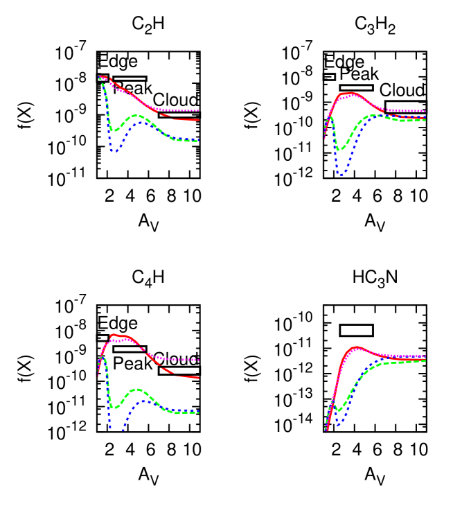
Figure 4: Fractional abundances of $\rm{C_{2}H}$, $\rm{c-C_{3}H_{2}}$, $\rm{C_{4}H}$, and $\rm{HC_{3}N}$ as functions of $A_{\rm{V}}$. The boxes represent observations with error bars, and the lines are the model results for $\zeta=10^{-17}$ s^-1 (blue dashed), $\zeta=10^{-15}$ s^-1 (pink dotted), and, from Figure 2, the mid-range $\zeta(N_{H})$ (green dashed) and high-range $\zeta(N_{H})$ (red solid).

Table 3: Abundance Ratios for Carbon-chain Species Between IR-peak and Cloud Regions

	IR-peak/Cloud
Species	Obs.	$\zeta(N_{H})$	$10^{-15}$ s-1
$\rm{C_{2}H}$	14	8.6	2.7
$c$–$\rm{C_{3}H_{2}}$	25	13	3.3
$\rm{C_{4}H}$	5	8	4

3.3 Results: $\rm{HC_{3}N}$, $\rm{HCO^{+}}$, $\rm{HCO}$ and the electron fraction

Only one line of the carbon-chain species HC₃N has been detected, and this with a very large beam-size (Teyssier et al., 2004). We follow Teyssier’s tabulated value for $A_{\rm V}$, and treat the emission as originating in the IR-peak, though there is some uncertainty about the origin of this emission. The four models all under-produce the observed abundance of $\rm{HC_{3}N}$ by a little less than an order of magnitude or more, as can be seen in Figure 4, with the models with the high-range $\zeta(N_{H})$ and the fixed $\zeta=10^{-15}$ s^-1 coming closest.

Cyanoacetylene ($\rm{HC_{3}N}$) is not as dependent as the other species on cosmic ray ionization for much of the range of visual extinction. Two reactions primarily lead to its formation:

$$\mathrm{CN}+\mathrm{C_{2}H_{2}}\rightarrow\mathrm{HC_{3}N}+\mathrm{H},$$

$$\mathrm{C_{3}H_{2}N^{+}}+e^{-}\rightarrow\mathrm{HC_{3}N}+\mathrm{H}.$$

At the edge, the first reaction is directly related to $\zeta$ through $\rm{C_{2}H_{2}}$, but the second reaction involves $\mathrm{C_{3}H_{2}N^{+}}$, the formation of which is not strongly dependent on $\zeta$. In the Cloud region, the situation is reversed: $\rm{C_{2}H_{2}}$ is less dependent on $\zeta$, and $\mathrm{C_{3}H_{2}N^{+}}$ is then closely linked with cosmic ray ionization. Because of the two channels for $\rm{HC_{3}N}$ we expect less dependence on $A_{\rm V}$ except in the middle range: $1<A_{\rm V}<5$. The results, shown in Figure 4, roughly bear this out. Interestingly, both the observed and calculated abundances for HC₃N are much lower than the initial value, which is taken from the TMC-1 abundance. The discrepancy with the Cloud value, over three orders of magnitude, is especially large and very different from the analogous cases for the hydrocarbons in Figure 4.

Figure 5 contains the observations and model results for $\rm{HCO^{+}}$ and HCO. Since HCO⁺ is optically thick, the carbon-13 isotopologue was used for observations. $\rm{H^{13}CO^{+}}$ was observed in emission at $\approx 40^{\prime\prime}$ from the PDR edge (Gerin et al., 2009), corresponding to an $A_{\rm{V}}\approx 10$, which is essentially the Cloud region. Following the analyses of Gerin et al. (2009) and Goicoechea et al. (2009b), we determined the abundance of $\rm{HCO^{+}}$ from $\rm{H^{13}CO^{+}}$ by assuming $\rm{{}^{12}C}/\rm{{}^{13}C}=60$. A faint emission feature attributed to $\rm{H^{13}CO^{+}}$ was also seen at $\approx 10^{\prime\prime}$ from the PDR edge, corresponding to an $A_{\rm{V}}\approx 2$ with our density profile, and so lies essentially at the IR-edge.

In the immediate neighborhood of $A_{\rm V}$ = 2, however, none of the models produces enough HCO⁺, but the increase in abundance with increasing extinction is steep and by $A_{\rm V}=3$, all but possibly the $\zeta=10^{-17}$ s^-1 model produce a comparable result to what is observed at the IR-edge. Goicoechea et al. (2009b) did much better fitting the $\rm{HCO^{+}}$ abundances at the edge by including PAH’s. They also modeled profiles for $\rm{H^{13}CO^{+}}$ and ${\rm DCO^{+}}$.

For the Cloud value, all models are in reasonable agreement with observation for HCO⁺, coming within factors of 2-5 of the observed abundance. The formation of $\rm{HCO^{+}}$ by cosmic rays is very direct at high extinction; in regions where UV photons cannot penetrate, it is almost solely the product of the destruction channel for protonated molecular hydrogen with carbon monoxide. At the IR-edge, however, the UV driven formation by the reactions $\rm{H_{2}+CO^{+}}$ and $\rm{H_{2}O+C^{+}}$ dominates. In all regions, $\rm{HCO^{+}}$ is destroyed mainly by recombination.

For neutral HCO, all model results are too low by an order of magnitude or more at both the IR-edge and Cloud regions, even with the relatively fast reaction between CH₂ and O (from Gerin et al., 2009). Our results disagree with the model results from Gerin et al. (2009) and Goicoechea et al. (2009b) partly because the Meudon reaction network includes a formation mechanism absent in the OSU network, the photodissociation reaction

$${\rm H_{2}CO}+h\nu\rightarrow{\rm HCO+H},$$ (15)

where $h\nu$ represents an external UV photon. This reaction is also discussed in Gerin et al. (2009). Including this reaction enhances the HCO abundance by a factor of $5$ in the PDR, bringing the HCO abundance within an order of magnitude of the observed value.

The ionization fraction, $f(e^{-})$, is a measure of elemental abundances, ionization rate, density, and chemistry, as well as a constraint on the coupling of the magnetic field to the matter in the cloud. The ionization fraction from our models, as shown in Figure 5, ranges from $\sim 10^{-4}$ in the PDR to $\sim 10^{-8}$ in the Cloud region. This range of fractions agrees generally with the profile in Goicoechea et al. (2009b, their Figure 4). Their inferred profile for the ionization fraction would favor the mid-range $\zeta(N_{H})$ from the cosmic ray flux-spectrum of Hayakawa et al. (1961).

For the steeper density profile with $\beta=4$ and the high $\zeta(N_{H})$, our results are somewhat different. The $\rm{HCO^{+}}$ abundances are not significantly changed, and the modeled $\rm{HCO}$ abundances increase by a factor of two in the IR-Edge and IR-Peak regions (at 10⁵ yr). Significantly, our calculated abundance of $\rm{HC_{3}N}$ comes into good agreement with the Cloud region observation; it is a factor of $3$ higher than the observed abundance at $t=10^{5}$ yr.

3.4 Tabulated Abundances

Calculated fractional abundances (with respect to $n_{\rm H}$) obtained with the standard elemental abundances are listed for more than twenty species in Table 4, including both observed and undetected molecules. The calculated results are for a time of 10⁵ yr and pertain to the center points of the IR-edge, IR-peak, and Cloud regions (Pety et al., 2005), for which observational results are also shown, when available. Some of the tabulated abundances, $\rm{HOC^{+}}$ especially, seem to be possible tracers for the cosmic ray ionization, because their fractional abundance becomes more dependent on the extinction when $\zeta$ depends on column density, than when $\zeta$ is a constant value.

In this table, we consider only the model with the high-range $\zeta(N_{H})$, because it is evident that, at least for carbon-chain species, use of this column-dependent $\zeta$ leads generally to better agreement with observations than models with lower ionization, and it is more physical than the constant high-ionization model. Also, we do not include the case of the steeper density profile in this table. Predictions are discussed below in Section 3.6.

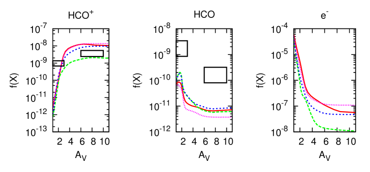
Figure 5: Relative abundances of $\rm{HCO^{+}}$, $\rm{HCO}$ and the ionization fraction as functions of $A_{\rm{V}}$. The boxes represent observations with error bars, and the lines are the model results for $\zeta=10^{-17}$ s^-1 (green dashed), $\zeta=10^{-15}$ s^-1 (pink dotted), and, from Figure 2, the mid-range $\zeta(N_{H})$ ( blue dotted) and high-range $\zeta(N_{H})$ (red solid).

Table 4: Observations and model results for fractional abundances at $10^{5}$ yr.

Species	IR-edge		IR-peak		Cloud
	Obs.	Mod.	Obs.	Mod.	Obs.	Mod.
O $\;(10^{-5})$		11		7.3		5.9
N $\;(10^{-6})$		16		1.1		1.3
CN $\;(10^{-8})$		2.3		1.0		0.2
NO $\;(10^{-9})$		0.07		77		103
O${}_{2}\;(10^{-7})$		$<$0.01		7.2		62
OH $\;(10^{-7})$		0.01		1.8		1.3
$\rm{CO}\;(10^{-5})$		6.0		9.6		9.9
$\rm{H_{2}O}\;(10^{-9})$		0.4		170		193
$\rm{C_{2}H}\;(10^{-8})$	3.3	1.6	3.0	0.3	0.2	0.07
$c$–$\rm{C_{3}H}\;(10^{-10})$		1.9	5.4	0.6		1.4
$l$–$\rm{C_{3}H}\;(10^{-10})$		1.0	2.9	8.0		0.9
$c$–$\rm{C_{3}H_{2}}\;(10^{-10})$	13	2.3	11	10	0.4	2.3
$\rm{C_{4}H}\;(10^{-9})$	9.5	1.3	3.6	2.0	0.8	0.1
$\rm{CH_{4}}\;(10^{-9})$		0.03		33		50
$\rm{C_{6}H}\;(10^{-11})$		1.4		4.1		0.2
$\rm{HCO}\;(10^{-10})$		0.03	17	0.1		0.2
$\rm{NH_{3}}\;(10^{-8})$		$<0.01$		1.2		2.5
$\rm{HCN}\;(10^{-10})$		0.8		40		26
$\rm{HNC}\;(10^{-10})$		0.9		67		17
$\rm{HC_{3}N}\;(10^{-11})$		$<0.01$	5.7	0.7		0.3
$\rm{HC_{5}N}\;(10^{-12})$		$<0.01$		4		0.13
$\rm{CH^{+}}\;(10^{-12})$		5		0.02		$<0.01$
$\rm{CO^{+}}\;(10^{-13})$	$\leq 5$	20		3.2		1.3
$\rm{HCO^{+}}\;(10^{-9})$	0.9	0.02		10	3.9	11
$\rm{HOC^{+}}\;(10^{-12})$	4	6		73		27
$\rm{OH^{+}}\;(10^{-13})$		4		15		5
$\rm{H_{2}O^{+}}\;(10^{-13})$		8		33		12
$\rm{H_{3}O^{+}}\;(10^{-10})$		0.1		45		37
$\rm{CH_{3}^{+}}\;(10^{-11})$		23		10		0.2
$\rm{C_{2}H_{4}^{+}}\;(10^{-13})$		1.5		19		12
$\rm{CS}\;(10^{-8})$	1.6	0.04	4.0	0.04		0.01
$\rm{HCS^{+}}\;(10^{-11})$		0.07	4.0	0.08		0.1

3.5 The Sulfur-Rich Case

We considered sulfur-bearing species, both with the standard initial abundances, and also for a sulfur-rich environment. We found that the higher the elemental sulfur (up to a relative abundance of $10^{-5}$), the closer the model matches observations for sulfur-bearing molecules. Our results and those of Goicoechea et al. (2006) for the chemistry and radiative transfer agree very well.

The results for the observed sulfur-bearing species CS and HCS⁺ vs $A_{\rm V}$ at 10⁵ yr can be found in Figure 6 as a function of the sulfur elemental abundance. There are two sets of curves, depending upon the rate coefficient for the charge-exchange reaction

$$\rm{S}+\rm{H^{+}}\rightarrow\rm{S^{+}}+\rm{H},$$

which can affect the abundances of CS and HCS⁺ at low sulfur abundances. This reaction has a listed rate coefficient of $1.3\times 10^{-9}$ cm³ s^-1 (Prasad & Huntress, 1980) but a more likely value of $1\times 10^{-14}$ cm³ s^-1 has been calculated.

The agreement attained by increasing the elemental abundance, $[\rm{S}]$, to $10^{-5}$ comes at a cost: at $10^{5}$ yr, all the carbon-bearing species in this scenario are reduced by up to a factor of 10 except at the IR-edge. This effect is most severe in the Cloud region. This depletion occurs in part because the high sulfur abundance destroys hydrocarbons by reactions with $\rm{S^{+}}$ and also with $\rm{S}$ at higher extinctions and because of the increased fractional ionization. The depletion of carbon-bearing species worsens agreement for all observed species except $\rm{HCO^{+}}$, which is brought to within a factor of $2$ of observation in the Cloud region.

This problem may suggest that a more realistic gas-phase sulfur elemental abundance for the Horsehead Nebula should lie somewhere around $10^{-6}$, in agreement with Goicoechea et al. (2006). The abundances of observed and predicted molecules with $[\rm{S}]=10^{-6}$ are in Table 5 for the same species as listed in Table 4. Even with this intermediate sulfur abundance, the calculated abundances of carbon chain species in particular are lowered considerably compared with the corresponding values in Table 4, leading to worse agreement with observation.

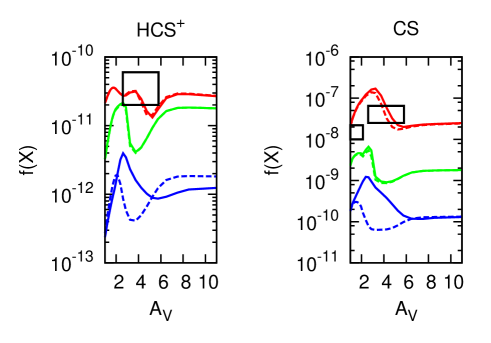
Figure 6: Relative abundances of $\rm{HCS^{+}}$ and $\rm{CS}$ as a function of $A_{\rm V}$. The boxes are the observations with error bars, and the lines are the model results with $[\rm{S}]=10^{-5}$ (red), $[\rm{S}]=10^{-6}$ (green) and $[\rm{S}]=7.2\times 10^{-8}$ (blue), all using the high column-dependent $\zeta$ from Figure 2. The solid lines use a rate for $\rm{S}+\rm{H^{+}}\rightarrow\rm{S^{+}}+\rm{H}$ of $1.3\times 10^{-9}$ cm³ s^-1 (Prasad & Huntress, 1980) and the dashed lines use a rate of $1\times 10^{-14}$ cm³ s^-1

3.6 Some Predictions

A high column-dependent $\zeta$ brings with it implications for chemistry in the Horsehead PDR. This column-dependent $\zeta$ varies from $\approx 2\times 10^{-16}$ s^-1 at the IR-edge to $\approx 7\times 10^{-17}$ s^-1 in the Cloud region and so leads to profiles distinctive from models with fixed ionization rates, as can be seen for carbon-chain species in Figures 4 to 6.

Also, other molecules are predicted to be in amounts in principle observable, and these are listed among the species in Tables 4 and 5. Because our $\zeta(N_{H})$ produces reasonable abundances of $\rm{C_{4}H}$ and $\rm{HC_{3}N}$ in selected regions with a low elemental abundance of sulfur, we would also expect to observe, albeit with some difficulty, the more complex carbon-chains $\rm{C_{6}H}$ and $\rm{HC_{5}N}$, based on our predictions for these regions. In addition, the molecule $\rm{HCN}$ should definitely be present in observable quantities, especially in inner regions, and its isomer, $\rm{HNC}$, should also be observed with a ratio $\rm{HCN}/\rm{HNC}\approx 1$. We predict ammonia in observable quantities at $A_{\rm V}>4$, for the low-sulfur case.

Given the observations of high amounts of the reactive molecular ions $\rm{OH^{+}}$ and $\rm{H_{2}O^{+}}$ in many molecular objects (Gerin et al., 2010; Gupta et al., 2010), it would be useful to consider predicted abundances of these species. Our model predictions for $\rm{OH^{+}}$, $\rm{H_{2}O^{+}}$ and ${\rm H_{3}O^{+}}$ in the Horsehead Nebula are contained in Tables 4 and 5. These predictions show low abundances for the first two ions that are rather independent of which of the three regions we consider. The basic problem is the low abundance of atomic hydrogen except at the border of the PDR (Neufeld et al., 2010). Even at the IR-Edge, ${\rm H_{3}O^{+}}$ is more than an order of magnitude higher than either OH⁺ or ${\rm H_{2}O^{+}}$, though none of these species should be sufficiently abundant to be detected. In the Cloud Region, where the electron density is at the low level of a cold dark cloud, ${\rm H_{3}O^{+}}$ is depleted rather slowly by reactions with electrons, and should achieve a high enough column to be detectable.

Table 5: Observations and model results for fractional abundances with $[\rm{S}]=10^{-6}$ at $10^{5}$ yr.

Species	IR-edge		IR-peak		Cloud
	Obs.	Mod.	Obs.	Mod.	Obs.	Mod.
O $\;(10^{-5})$		12		9.9		4.9
N $\;(10^{-6})$		16		1.3		0.3
CN $\;(10^{-8})$		1.1		0.08		0.02
NO $\;(10^{-9})$		0.1		69		123
O${}_{2}\;(10^{-7})$		$<$0.01		18		260
OH $\;(10^{-7})$		0.01		1.0		1.0
$\rm{CO}\;(10^{-5})$		5.5		7.3		7.3
$\rm{H_{2}O}\;(10^{-9})$		0.4		420		390
$\rm{C_{2}H}\;(10^{-8})$	3.3	1.1	3.0	0.3	0.2	$<0.01$
$c$–$\rm{C_{3}H}\;(10^{-10})$		1.8	5.7	0.2		0.01
$l$–$\rm{C_{3}H}\;(10^{-10})$		1.0	2.9	0.1		$<$0.01
$c$–$\rm{C_{3}H_{2}}\;(10^{-10})$	13	2	11	0.4	0.4	0.03
$\rm{C_{4}H}\;(10^{-9})$	9.5	0.7	3.6	0.1	0.8	$<0.01$
$\rm{CH_{4}}\;(10^{-9})$		0.05		30		22
$\rm{C_{6}H}\;(10^{-11})$		1.2		$<0.01$		$<0.01$
$\rm{HCO}\;(10^{-10})$		0.9	17	0.5		0.06
$\rm{NH_{3}}\;(10^{-8})$		$<$0.01		$<$0.01		$<$0.01
$\rm{HCN}\;(10^{-10})$		0.6		18		10
$\rm{HNC}\;(10^{-10})$		0.9		39		27
$\rm{HC_{3}N}\;(10^{-11})$		$<$0.01	5.7	0.03		0.01
$\rm{HC_{5}N}\;(10^{-12})$		$<$0.01		$<$0.01		$0.01$
$\rm{CH^{+}}\;(10^{-12})$		2.9		$<0.01$		$<0.01$
$\rm{CO^{+}}\;(10^{-13})$	$\leq 5$	1.5		0.7		0.5
$\rm{HCO^{+}}\;(10^{-9})$	0.9	0.02		0.7	3.9	6.2
$\rm{HOC^{+}}\;(10^{-12})$	4	4		20		10
$\rm{OH^{+}}\;(10^{-13})$		3.1		9.3		3.6
$\rm{H_{2}O^{+}}\;(10^{-13})$		5.3		15		7.4
$\rm{H_{3}O^{+}}\;(10^{-10})$		0.1		50		40
$\rm{CH_{3}^{+}}\;(10^{-11})$		20		3.2		0.3
$\rm{C_{2}H_{4}^{+}}\;(10^{-13})$		2.1		3.2		0.8
$\rm{CS}\;(10^{-8})$	1.6	0.5	4.0	0.9		0.2
$\rm{HCS^{+}}\;(10^{-11})$		1.1	4.0	1.8		1.7

4 Discussion

We have modeled the Horsehead Nebula as a PDR with time-dependent gas-phase chemistry using a column-dependent cosmic ray ionization rate $\zeta(N_{H})$, as well as the temperature and density profiles of Habart et al. (2005). At a cloud age of 10⁵ yr, the incorporation of a high $\zeta(N_{H})$ improves agreement between model and observation for the small carbon-bearing molecules $\rm{HCO^{+}}$, $\rm{HC_{3}N}$, $\rm{C_{2}H}$, $\rm{c-C_{3}H_{2}}$, and $\rm{C_{4}H}$ compared with a more standard constant ionization rate. With a higher abundance of elemental sulfur than our standard value, the results for small sulfur-bearing species are improved, but at the expense of our calculated values for carbon-chain species. There are also predictions of abundances and profiles for other species, some not yet observed in the Horsehead Nebula, which should be in principle observable, including HCN, HNC, NH₃, $\rm{C_{6}H}$, $\rm{HC_{5}N}$, and $\rm{H_{3}O^{+}}$. Some of these predictions are strongly affected, however, by an increase in the assumed sulfur elemental abundance.

Our results for c-C₃H₂ and C₄H (but not for C₂H) also indicate that the fracturing of PAH’s may play an important role in the production of these molecules towards the edge of the PDR, but our model does not incorporate the effects of PAH’s. Strong aromatic emission, observed by Compiègne et al. (2007), poses some problems, however, for the hypothesis that PAH fracturing is the source of small hydrocarbons. These authors claim a high concentration of neutral PAH’s in the HII region, which suggests that PAH’s may endure the radiation at the IR-edge, instead of breaking apart into the observed hydrocarbons.

The detailed form of the calculated abundance profiles in Figures 4 through 6 cannot be observed because observations up to the present lack sufficient resolution, and because the density profile is not well-determined. With the advent of the Atacama Large Millimeter Array (ALMA), the estimated increase in angular resolution, to $\sim 0.1^{\prime\prime}$ (Wootten, 2003), should allow us to observe the form of these abundance profiles, so as to better determine the initial flux-spectrum for cosmic rays for the Horsehead Nebula.

It appears, from Indriolo et al. (2010), that there is some environmental influence on the low energy flux of cosmic rays. It would be of great interest to not only examine the Horsehead Nebula at greater angular resolution, but to also observe and model other PDR’s such as the Orion Bar, IC-63, L1688-W, and portions of Sgr B2 to determine how the low energy cosmic ray flux varies in our Galaxy. Sgr B2 is of special interest given the high values of $\zeta$ inferred from H${}_{3}^{+}$ observations in this region (Oka et al., 2005). Given the strong dependence of $\zeta$ on the path cosmic rays travel, it is very likely that the low-energy cosmic ray flux will be object-dependent.