Finite size emptiness formation probability of the XXZ spin chain at $\Delta=-\frac{1}{2}$

In this paper we compute the Emptiness Formation Probability of a (twisted-) periodic XXZ spin chain of finite length at $\Delta=-\frac{1}{2}$, thus proving the formulas conjectured by Razumov and Stroganov [3, 4]. The result is obtained by exploiting the fact that the ground state of the inhomogeneous XXZ spin chain at $\Delta=-\frac{1}{2}$ satisfies a set of qKZ equations associated to $\displaystyle{U_{q}(\hat{sl_{2}})}$.

1 Introduction

The computation of correlation functions in quantum integrable systems, is in general a quite hard task. One paradigmatic example is the spin-$\frac{1}{2}$ XXZ spin chain [1]. Even in the study of the free fermion case quite interesting mathematical structures have appeared [2]. Starting from the seminal papers of Razumov and Stroganov [3, 4], we know that the anti-ferromagnetic ground state of the XXZ spin chain at the value $\Delta=-\frac{1}{2}$ of the anisotropy parameter (or equivalently $q=e^{2\pi i/3}$) presents a remarkable combinatorial structure. The spin chain hamiltonians with an odd number of spins $N=2n+1$ and periodic boundary conditions or even number of spins $N=2n$ and twisted-periodic boundary conditions are related through a change of basis to the Markov matrix of a stochastic loop model [5]. In the loop basis, the “ground state” is actually the steady state probability of the stochastic loop model. The most astonishing discovery was made by Razumov and Stroganov [6], who observed that, once properly normalized, the components of the steady state are integer numbers enumerating Fully Packed Loop configurations on a square grid. This conjecture has been eventually proven in [7].

Despite being the XXZ spin chain at $\Delta=-\frac{1}{2}$ a fully interacting system, several of its correlation functions have simple exact formulate even at finite size. This is the case of the Emptiness Formation Probability (in short EFP), which is the probability that $k$ consecutive spins are in the up direction in a chain of length $N$. In their original papers [3, 4], Razumov and Stroganov have conjectured exact factorized formulas for the EFP in terms of products of factorials. The aim of the present paper is to prove these conjectures.

The XXZ spin chain with odd size has two ground states $\Psi^{+}_{2n+1}$ and $\Psi^{-}_{2n+1}$, related by a spin flip on each site. Razumov and Stroganov have conjectured [3] that $E^{-}_{2n+1}(k)$, the EFP of a k-string of spins up in the state $\Psi^{-}_{2n+1}$, satisfies

$$\frac{E_{2n+1}^{-}(k-1)}{E^{-}_{2n+1}(k)}=\frac{(2k-2)!(2k-1)!(2n+k)!(n-k)!}{(k-1)!(3k-2)!(2n-k+1)!(n+k-1)!}.$$ (1)

Strangely enough, Razumov and Stroganov didn’t provide the analogous formula for the state $\Psi^{+}_{2n+1}$, which reads

$$\frac{E^{+}_{2n+1}(k-1)}{E^{+}_{2n+1}(k)}=\frac{(2k-2)!(2k-1)!(2n+k)!(n-k+1)!}{(k-1)!(3k-2)!(2n-k+1)!(n+k)!}$$ (2)

In particular, the probability of having a string of spins-up of length $n$ (or $n+1$) in a chain of length $2n+1$ is equal to the inverse of $A_{HT}(2n+1)$, the number of of Half Turn Symmetric Alternating Sign Matrices of size $2n+1$,

$$E_{2n+1}^{-}(n)=E_{2n+1}^{+}(n+1)=A_{HT}(2n+1)^{-1}=\prod_{j=1}^{n}\frac{(2j-1)!^{2}(2j)!^{2}}{(j-1)!j!(3j-1)!(3j)!}$$ (3)

In the case of a spin chain with even length and twisted boundary conditions, the ground state is unique. Razumov and Stroganov have conjectured [4] that $E^{e}_{2n}(k)$, the EFP of a k-string of spins up satisfies

$$\frac{E^{e}_{2n}(k-1)}{E^{e}_{2n}(k)}=\frac{(2k-2)!(2k-1)!(2n+k-1)!(n-k)!}{(k-1)!(3k-2)!(2n-k)!(n+k-1)!}$$ (4)

The previous equation implies that in the case $k=n$

$$E^{e}_{2n}(k)=A_{HT}(2n)^{-1}.$$ (5)

Unlike the ground states of the odd size chains, whose components can be chosen to be real, the even size ground state has complex valued components, therefore we can consider also $E^{\tilde{e}}_{2n}(k)$, a sort of “pseudo” EFP obtained by sandwiching the ground state with itself (and not with its complex conjugate). The ratio of “pseudo” EFPs corresponding to the same size of the spin chain has a factorized form given by

$$\frac{E^{\tilde{e}}_{2n}(k-1)}{E^{\tilde{e}}_{2n}(k)}=-q\frac{(2k-2)!(2k-1)!(2n+k-1)!(n-k)!}{(k-1)!(3k-3)!(3k-1)(2n-k)!(n+k-1)!}.$$ (6)

It turns out that, apart for the factor $-q$, the ratio in eq.(6) can be written as a ratio of enumerations of $k$-Punctured Cyclically Symmetric Self-Complementary Plane Partitions (PCSSCPP) of size $2n$, i.e. rhombus tilings of a regular hexagon of side length $2n$, which are symmetric under a $\pi/3$ rotation around the center of the hexagon and with a star shaped frozen region of size $k$, as exemplified in Figure 1.

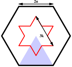
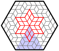
Figure 1: Domain tiled by $k$-Punctured Cyclically Symmetric Self-Complementary Plane Partitions, with an example of tiling for $n=3$ and $k=2$. The shadowed region indicates a fundamental domain.

Calling these enumerations $CSSCPP(2n,k)$ we have

$$\frac{E^{\tilde{e}}_{2n}(k-1)}{E^{\tilde{e}}_{2n}(k)}=-q\frac{CSSCPP(2n,k-1)}{CSSCPP(2n,k)}.$$ (7)

For $k=n$ one obtains

$$E^{\tilde{e}}_{2n}(n)=(-q)^{n}A_{n}^{-2}=(-q)^{n}CSSCPP(2n)^{-1}$$ (8)

where $A_{n}$ is the number of Alternating Sign Matrices of size $n$

$$A_{n}=\prod_{j=0}^{n-1}\frac{(3j+1)!}{(n+j)!},$$ (9)

and $CSSCPP(2n)$ is the number of Cyclically Symmetric Self-Complementary Plane Partitions in an hexagon of size $2n$. The enumerations $CSSCPP(2n,k)$ are easily computed by applying a result of Ciucu [10] concerning enumerations of dimer coverings of planar graphs with reflection symmetry. This will be explained briefly in Appendix B.

Some partial results concerning the (pseudo)-norm, and the EFP have been obtained in the literature. In [11], by cleverly exploiting the relation between a natural degenerate scalar product in the loop basis and the usual scalar product in the spin basis, Di Francesco and collaborators have proven eq.(3) and eq.(8).

In the large $N$ limit $N\rightarrow\infty$, the EFP have been studied Maillet and collaborators [12]. Of course the conjectures (1, 2, 4) must coincide and must give for the thermodynamic limit of the EFP

$$\lim_{N\rightarrow\infty}E_{N}(k)=\left(\frac{\sqrt{3}}{2}\right)^{3k^{2}}\prod_{j=1}^{k}\frac{\Gamma(j-1/3)\Gamma(j+1/3)}{\Gamma(j-1/2)\Gamma(j+1/2)}.$$ (10)

This formula has been proven in [12] by specializing to $\Delta=-\frac{1}{2}$ a multiple integral representation for the correlation functions, which is valid for generic values of the anisotropy parameter $\Delta$.

The most effective technique which has allowed to compute (partial) sum of components in the loop or in the spin basis has been pushed forward by Di Francesco and Zinn-Justin [8] in the context of the periodic loop model with an even number of sites. They introduced spectral parameters in the model in such a way to preserve its integrability, the original model being recovered once the spectral parameters are set to $1$. In this way the components of the ground state become homogeneous polynomials in the spectral parameters, which satisfy certain relation under exchange or specialization of the spectral parameters. As noticed first by Pasquier [14] and largely developed by Di Francesco and Zinn-Justin [15] the exchange relations satisfied by the ground state are a special case ($q=e^{2\pi i/3}$) of the very much studied quantum Knizhnik–Zamolodchikov equations (qKZ) [16]. In [17] the authors have applied this idea to the XXZ spin chain with spectral parameters and have shown that the properly normalized ground state of the spin chain with periodic or twisted periodic boundary conditions satisfies a special case of the $U_{q}(sl_{2})$ qKZ equations at level $1$. Here we employ this property in order to compute the Emptiness Formation Probability. Our main idea is to consider a generalization of the EFP with spectral parameters EFP, which is constructed from the solution of the $U_{q}(sl_{2})$ qKZ equations for generic $q$ (see eqs.(48,49). This “inhomogeneous” EFP has certain symmetry and recursion properties that completely fix it in the same spirit as the recursion relations of the 6-vertex model with Domain Wall Boundary Conditions completely determine its partition function. This will allow us to present an explicit determinantal formula for the inhomogeneous EFP valid at $q=e^{2\pi i/3}$, and upon specialization of the spectral parameters will allow to obtain the formulas (1, 2, 4, 6).

The idea to use the solution of the qKZ equation to compute the inhomogenous version of a correlation function can be in principle adapted to several other models like: XXZ spin chain with different boundary conditions, fused XXZ spin chain, $U_{q}(sl_{n})$ spin chain or even XYZ spin chain etc. [20, 21, 22, 23]. Indeed, in all these cases, by properly tuning the parameters (generalizing the relation $q=e^{2\pi i/3}$), one has a so called “combinatorial point” at which the ground state energy per site doesn’t get finite size corrections. By reasonings similar to the one in [17], one can argue that the ground state with spectral parameters satisfies a qKZ equation (or, in the case of the XYZ spin chain, an elliptic version of it).

Whether this idea could lead to other exact finite size formulae for some correlation function is an open question that in our opinion deserves further investigation.

The paper is organized as follows. In Section 2, after having recalled some basic facts about the XXZ spin chain, following [17] we present the exchange equations satisfied by the ground state at $\Delta=-\frac{1}{2}$, then in Section 2.2 we derive the recursion relations satisfied by the solutions of the $U_{q}(sl_{2})$ qKZ equations at level $1$. In Section 3 we define the inhomogeneous version of the (pseudo) EFP, constructed using the solutions of the qKZ equations. We derive first its symmetries and then in Section 3.1 we derive the recursion relations which completely determine it. In section 4 we will restrict to $q=e^{2\pi i/3}$ and, by showing that certain determinantal expressions satisfy the same recursion relations as the inhomogeneous EFP, we produce a representation of this inhomogeneous EFP whose homogeneous specialization is considered in Section 4.1, where we prove the main conjectures. In Appendix A we compute the determinants of a family of matrices which are relevant for the computation of the homogeneous specialization considered in Section 4.1. In Appendix B we compute the lozenge tilings enumerations $CSSCPP(2n,k)$.

2 XXZ spin chain at $\Delta=-\frac{1}{2}$ and qKZ equations

The hamiltonian of the XXZ spin chain acts on a vector space $\mathcal{H}_{N}=(\mathbb{C}^{2})^{\otimes N}$ that consists of $N$ copies of $\mathbb{C}^{2}$ each one labeled by an index $i$. The hamiltonian is written in terms of operators $\sigma^{\alpha}_{i}$ which are Pauli matrices acting locally on the $i$-th component $\mathbb{C}_{i}^{2}$

$$H_{N}(\Delta)=-\frac{1}{2}\sum_{i=1}^{N}\sigma^{x}_{i}\sigma^{x}_{i+1}+\sigma^{y}_{i}\sigma^{y}_{i+1}+\Delta\sigma^{z}_{i}\sigma^{z}_{i+1}.$$ (11)

It is convenient to parametrize the anisotropy parameter as $\Delta=\frac{q+q^{-1}}{2}$. The model is completely specified once the boundary conditions are provided. Here we will consider:

• periodic boundary conditions for odd values of the length of the spin chain, $N=2n+1$, i.e. $\sigma_{N+1}^{\alpha}=\sigma_{1}^{\alpha}$

• twisted periodic boundary conditions for even values of the length of the spin chain, $N=2n$, i.e. $\sigma_{N+1}^{z}=\sigma_{1}^{z}$, while $\sigma^{\pm}_{N+1}=e^{\pm i\frac{2\pi}{3}}\sigma^{\pm}_{N+1}$, where $\sigma^{\pm}=\sigma^{x}+\pm i\sigma^{y}$.

It is well know [1] that the Hamiltonian (11), for generic values of the parameter $\Delta$ and of the twisting, is the logarithmic derivative of an integrable transfer matrix. In order to define the transfer matrix we need the $R$-matrix and the twist matrix. In the present context the $R$-matrix is an operator depending on a spectral parameter $z$, which acts on a tensor product $\mathbb{C}^{2}_{i}\otimes\mathbb{C}^{2}_{j}$. Introducing the basis of $\mathbb{C}_{i}^{2}$

$$e^{\uparrow}_{i}=\left(\begin{array}[]{c}1\\ 0\end{array}\right),\leavevmode\nobreak\ \leavevmode\nobreak\ \leavevmode\nobreak\ e^{\downarrow}_{i}=\left(\begin{array}[]{c}0\\ 1\end{array}\right).$$

we write $R_{i,j}(z)$ in the basis $\{e^{\uparrow}_{i}\otimes e^{\uparrow}_{j},e^{\uparrow}_{i}\otimes e^{\downarrow}_{j},e^{\downarrow}_{i}\otimes e^{\uparrow}_{j},e^{\downarrow}_{i}\otimes e^{\downarrow}_{j}\}$ of $\mathbb{C}_{i}^{2}\otimes\mathbb{C}^{2}_{j}$ as

$$R_{i,j}(z)=\left(\begin{array}[]{cccc}a(z)&0&0&0\\ 0&b(z)&c_{1}(z)&0\\ 0&c_{2}(z)&b(z)&0\\ 0&0&0&a(z)\end{array}\right)$$ (12)

with

$$a(z)=\frac{qz-q^{-1}}{q-q^{-1}z},\leavevmode\nobreak\ \leavevmode\nobreak\ \leavevmode\nobreak\ \leavevmode\nobreak\ b(x)=\frac{z-1}{q-q^{-1}z},\leavevmode\nobreak\ \leavevmode\nobreak\ \leavevmode\nobreak\ \leavevmode\nobreak\ c_{1}(z)=\frac{(q-q^{-1})z}{q-q^{-1}z},\leavevmode\nobreak\ \leavevmode\nobreak\ \leavevmode\nobreak\ \leavevmode\nobreak\ c_{2}(z)=\frac{(q-q^{-1})}{q-q^{-1}z}.$$ (13)

The twist matrix $\Omega(\phi)$ acts on a single $\mathbb{C}_{i}^{2}$ and in the basis $(e^{\uparrow}_{i},e^{\downarrow}_{i}$) it reads

$$\Omega(\phi)=\left(\begin{array}[]{cc}e^{i\phi}&0\\ 0&e^{-i\phi}\end{array}\right).$$ (14)

Using both the twist and the $R$-matrix we construct the family of transfer matrices

$$T_{N}(y|{\bf z}_{\{1,\dots,N\}},\phi)={\rm tr}_{0}\left[R_{0,1}(y/z_{1})R_{0,2}(y/z_{2})\dots R_{0,N}(y/z_{N})\Omega_{0}(\phi)\right]$$ (15)

depending on $N$ “vertical” spectral parameters ${\bf z}_{\{1,\dots,N\}}$ and a single “horizontal” spectral parameter $y$. Thanks to the commutation relation

$$[R_{i,j}(x),\Omega_{i}(\phi)\otimes\Omega_{j}(\phi)]=0$$ (16)

and the Yang-Baxter equation

$$R_{i,j}(z_{i}/z_{j})R_{i,k}(z_{i}/z_{k})R_{j,k}(z_{j}/z_{k})=R_{j,k}(z_{j}/z_{k})R_{i,k}(z_{i}/z_{k})R_{i,j}(z_{i}/z_{j})$$ (17)

the transfer matrices for different values of $y$ commute

$$[T_{N}(y^{\prime}|{\bf z}_{\{1,\dots,N\}},\phi),T_{N}(y^{\prime\prime}|{\bf z}_{\{1,\dots,N\}},\phi)]=0.$$ (18)

The hamiltonian of the XXZ spin chain is given by

$$\frac{1}{T_{N}(1|{\bf 1},\phi)}\frac{dT_{N}(y|{\bf 1},\phi)}{dy}{\Bigg{|}}_{y=1}=-\frac{1}{q-q^{-1}}\left(H_{N}(\Delta)-\frac{3N}{2}\Delta\right).$$ (19)

At $\Delta=-\frac{1}{2}$ and for generic values of the vertical spectral parameters, both in the odd size case with periodic boundary conditions and in the even size case with twisted boundary conditions, the transfer matrix has an eigenvalue equal to $1$.

• When $N=2n+1$, the eigenspace with eigenvalue $1$ is two-fold degenerate, $\Psi^{\pm}_{2n+1}({\bf z})$, corresponding to two the values $\pm\frac{1}{2}$ of the total spin $S^{z}=\frac{1}{2}\sum_{i=1}^{N}\sigma^{z}_{i}$

  $$S^{z}\Psi^{\pm}_{2n+1}({\bf z})=\pm\Psi^{\pm}_{2n+1}({\bf z})$$ (20)

  The two eigenstates are related by a flipping of all the spins

  $$\Psi^{+}_{2n+1}({\bf z})=\prod_{i=1}^{N}\sigma^{x}_{i}\cdot\Psi^{-}_{2n+1}({\bf z}).$$ (21)

• When $N=2n$ there is a single vector $\Psi^{e}_{2n}({\bf z})$ with eigenvalue $1$. It is in the zero sector of the total spin,

  $$S^{z}\Psi^{e}_{2n}({\bf z})=0,$$ (22)

  These eigenstates reduce to the anti-ferromagnetic ground state(s) of the XXZ spin chain when the spectral parameters are specialized at $z_{i}=1$.

2.1 Exchange relations at $\Delta=-\frac{1}{2}$

A crucial observation made in [17] was that, for an appropriate choice of the normalization of $\Psi^{\mu}_{N}({\bf z})$, the eigenvector equation

$$T_{N}(y|{\bf 1},\phi)\Psi^{\mu}_{N}({\bf z})=\Psi^{\mu}_{N}({\bf z})$$ (23)

is equivalent to a set of exchange relations. Define the exchange operator $P_{i,j}(e^{\mu}_{i}\otimes e^{\nu}_{j})=e^{\nu}_{i}\otimes e^{\mu}_{j}$, the left rotation operator $\sigma(v_{1}\otimes v_{2}\otimes\cdots\otimes v_{N-1}\otimes v_{N})=v_{2}\otimes\cdots\otimes v_{N-1}\otimes v_{N}\otimes v_{1}$ and let $\check{R}_{i,i+1}(z)=P_{i,i+1}R_{i,i+1}(z)$, then $\Psi^{\mu}_{N}({\bf z})$, as a polynomial of minimal degree in the spectral parameters $z_{i}$, is determined up to a constant factor, by the following set of equations [17]

$$\check{R}_{i,i+1}(z_{i+1}/z_{i})\Psi^{\mu}_{N}(z_{1},\dots,z_{i},z_{i+1},\dots,z_{N}) =\Psi^{\mu}_{N}(z_{1},\dots,z_{i+1},z_{i},\dots,z_{N})$$ (24)

$$\sigma\Psi^{\mu}_{N}(z_{1},z_{2},\dots,z_{N-1},z_{N}) =D\Psi^{\mu}_{N}(z_{2},\dots,z_{N-1},z_{N},sz_{1}).$$ (25)

with $D=s=1$. These equations can be seen as the special case $q=e^{2\pi i/3}$ of the level $1$ qKZ equations [16], which corresponds to generic $q$, $s=q^{6}$ and $D=q^{3N}q^{3(s^{z}_{N}+1)/2}$. The solution of the level $1$ qKZ equations can be normalized in such a way that they become polynomials in the variables $z_{i}$ [17] of degree $n-1$ in the case of even size $N=2n$, and degree $n$ in the odd case $N=2n+1$.

Using the projectors $p_{i}^{\pm}=\frac{1\pm\sigma_{i}^{z}}{2}$ of the $i$-th spin in the up/down direction, let us write the exchange eqs.(24) in components. If we have a spin up at site $i$ and a spin down at site $i+1$ or viceversa, we have

$$\begin{split}p_{i}^{-}p_{i+1}^{+}\Psi^{\mu}(z_{i},z_{i+1})&=\sigma_{i}^{-}\sigma_{i+1}^{+}\frac{(qz_{i}-q^{-1}z_{i+1})\Psi^{\mu}(z_{i+1},z_{i})-(q-q^{-1})z_{i}\Psi^{\mu}(z_{i},z_{i+1})}{z_{i+1}-z_{i}}\\ p_{i}^{+}p_{i+1}^{-}\Psi^{\mu}(z_{i},z_{i+1})&=\sigma_{i}^{+}\sigma_{i+1}^{-}\frac{(qz_{i}-q^{-1}z_{i+1})\Psi^{\mu}(z_{i+1},z_{i})-(q-q^{-1})z_{i+1}\Psi^{\mu}(z_{i},z_{i+1})}{z_{i+1}-z_{i}}\end{split}$$ (26)

These equations form a triangular system. Starting from a given component we can reconstruct all the others repeatedly using eqs.(26). Therefore if we want to show that two a priori distinct solutions of the qKZ equations actually coincide, it is enough to check the equality of one of their components.

When there are two consecutive spins pointing in the same direction at positions $i$ and $i+1$, then the first of the qKZ equations reads

$$\begin{split}p_{i}^{\pm}p_{i+1}^{\pm}\Psi^{\mu}(\dots,z_{i+1},z_{i},\dots)=\frac{qz_{i+1}-q^{-1}z_{i}}{qz_{i}-q^{-1}z_{i+1}}p_{i}^{\pm}p_{i+1}^{\pm}\Psi^{\mu}(\dots,z_{i},z_{i+1},\dots)\end{split}$$ (27)

which means that the components having two consecutive spins up or down at positions $i$ and $i+1$, $p_{i}^{\pm}p_{i+1}^{\pm}\Psi^{\mu}(\dots,z_{i+1},z_{i},\dots)$ have a factor $qz_{i}-q^{-1}z_{i+1}$

$$p_{i}^{\pm}p_{i+1}^{\pm}\Psi^{\mu}(\dots,z_{i},z_{i+1},\dots)=(qz_{i}-q^{-1}z_{i+1})\tilde{\Psi}^{\mu,\pm}_{i,i+1}(\dots,z_{i},z_{i+1},\dots)$$ (28)

and the vectors $\tilde{\Psi}^{\mu,\pm}_{i,i+1}(\dots,z_{i},z_{i+1},\dots)$ are symmetric under exchange $z_{i}\leftrightarrow z_{i+1}$. Another useful relation is obtained by considering the matrix $e_{i}$, which is proportional to a projector and is a generator of the Temperley-Lieb algebra

$$e_{i}=\left(\begin{array}[]{cccc}0&0&0&0\\ 0&-q&1&0\\ 0&1&-q^{-1}&0\\ 0&0&0&0\end{array}\right),\leavevmode\nobreak\ \leavevmode\nobreak\ \leavevmode\nobreak\ \leavevmode\nobreak\ \leavevmode\nobreak\ \leavevmode\nobreak\ \leavevmode\nobreak\ \leavevmode\nobreak\ \leavevmode\nobreak\ \leavevmode\nobreak\ \leavevmode\nobreak\ \leavevmode\nobreak\ \begin{array}[]{l}e_{i}^{2}=\tau e_{i},\leavevmode\nobreak\ \leavevmode\nobreak\ \leavevmode\nobreak\ \leavevmode\nobreak\ \tau=-q-q^{-1}\\[5.0pt] e_{i}e_{i\pm 1}e_{i}=e_{i}\\[5.0pt] e_{i}e_{j}=e_{j}e_{i}\leavevmode\nobreak\ \leavevmode\nobreak\ \leavevmode\nobreak\ \textrm{for}\leavevmode\nobreak\ \leavevmode\nobreak\ \leavevmode\nobreak\ \leavevmode\nobreak\ |i-j|>1\end{array}$$ (29)

The matrix $e_{i}$ is preserved under multiplication by a $\check{R}$-matrix for any value of the spectral parameter

$$e_{i}\check{R}_{i,i+1}(z)=\check{R}_{i,i+1}(z)e_{i}=e_{i}.$$ (30)

By applying $e_{i}$ to the left of the first of the qKZ eqs.(24) we find

$$e_{i}\Psi^{\mu}(\dots,z_{i},z_{i+1},\dots)=e_{i}\Psi^{\mu}(\dots,z_{i+1},z_{i},\dots).$$ (31)

The components with most consecutive aligned spins have a completely factorized form

$$\begin{split}\Psi^{e}_{\underbrace{\uparrow,\dots,\uparrow}_{n},\underbrace{\downarrow,\dots,\downarrow}_{n}}({\bf z})&=\prod_{1\leq i<j\leq n}\frac{qz_{i}-q^{-1}z_{j}}{q-q^{-1}}\prod_{n+1\leq i<j\leq 2n}\frac{qz_{i}-q^{-1}z_{j}}{q-q^{-1}}\\ \Psi^{+}_{\underbrace{\uparrow,\dots,\uparrow}_{n+1},\underbrace{\downarrow,\dots,\downarrow}_{n}}({\bf z})&=\prod_{1\leq i<j\leq n+1}\frac{qz_{i}-q^{-1}z_{j}}{q-q^{-1}}\prod_{n+2\leq i<j\leq 2n+1}\frac{qz_{i}-q^{-1}z_{j}}{q-q^{-1}}\prod_{i=n+2}^{2n+1}z_{i}\\ \Psi^{-}_{\underbrace{\uparrow,\dots,\uparrow}_{n},\underbrace{\downarrow,\dots,\downarrow}_{n+1}}({\bf z})&=\prod_{1\leq i<j\leq n}\frac{qz_{i}-q^{-1}z_{j}}{q-q^{-1}}\prod_{n+1\leq i<j\leq 2n+1}\frac{qz_{i}-q^{-1}z_{j}}{q-q^{-1}}\end{split}$$ (32)

where the residual normalization ambiguity has been fixed by requiring these components to be equal to $1$ for $z_{i}=1$. From eqs.(32) we see that the maximally factorized components satisfy (among others) the following relations

$$\begin{split}\Psi^{+}_{\underbrace{\uparrow,\dots,\uparrow}_{n+1},\underbrace{\downarrow,\dots,\downarrow}_{n}}({\bf z})&=(1-q^{-2})^{n}\Psi^{e}_{\underbrace{\uparrow,\dots,\uparrow}_{n+1},\underbrace{\downarrow,\dots,\downarrow}_{n+1}}({\bf z})|_{z_{2n+2}=0}\\[5.0pt] \Psi^{e}_{\underbrace{\uparrow,\dots,\uparrow}_{n},\underbrace{\downarrow,\dots,\downarrow}_{n}}({\bf z})&=(1-q^{2})^{n}\lim_{z_{2n+1}\rightarrow\infty}z_{2n+1}^{-n}\Psi^{-}_{\underbrace{\uparrow,\dots,\uparrow}_{n},\underbrace{\downarrow,\dots,\downarrow}_{n+1}}({\bf z})\end{split}.$$ (33)

Using the triangularity of the eqs.(26) we can conclude that the eqs.(33) induce equalities between components of $\Psi^{+}_{2n+1}({\bf z})$ or $\Psi^{e}_{2n}({\bf z})$ and components of $\Psi^{e}_{2n+2}({\bf z})$ or $\Psi^{-}_{2n+1}({\bf z})$ with the last spin down, i.e.

$$\begin{split}\Psi^{+}_{2n+1}({\bf z})\otimes e_{2n+2}^{\downarrow}&=(1-q^{-2})^{n}p^{-}_{2n+2}\Psi^{e}_{2n+2}({\bf z})|_{z_{2n+2}=0}\\ \Psi^{e}_{2n}({\bf z})\otimes e_{2n+1}^{\downarrow}&=(1-q^{2})^{n}\lim_{z_{2n+1}\rightarrow\infty}z_{2n+1}^{-n}p^{-}_{2n+1}\Psi^{-}_{2n+1}({\bf z})\end{split}$$ (34)

We will use these equations in order to find a relation among the inhomogeneous versions of the EFP that we shall introduce in Section 3.

2.2 Recursion relation

We claim that, upon specialization $z_{i+1}=q^{2}z_{i}$ the solution of the qKZ equation for $N$ spins reduces to the solution of the same system of equations for $N-2$ spins. In order to make the previous statement more precise we need to introduce some notation. Let $v_{i}$ be the vectors which are in the image of the projectors proportional to the generator of the Temperley-Lieb algebra $e_{i}$

$$v_{i}=e_{i}^{\uparrow}\otimes e_{i+1}^{\downarrow}-q^{-1}e_{i}^{\downarrow}\otimes e_{i+1}^{\uparrow},\leavevmode\nobreak\ \leavevmode\nobreak\ \leavevmode\nobreak\ \leavevmode\nobreak\ \leavevmode\nobreak\ \leavevmode\nobreak\ e_{i}v_{i}=-(q+q^{-1})v_{i}$$ (35)

Introduce the injective map

$$\Phi_{N}^{(i)}:(\mathbb{C}^{2})^{\otimes N}\rightarrow(\mathbb{C}^{2})^{\otimes N+2},$$ (36)

which inserts the vector $v_{i}$ at position $(i,i+1)$ and shift by two steps the indices of the sites with $j\geq i$, i.e. on a basis

$$\Phi_{N}^{(i)}(e_{1}^{a_{1}}\otimes\cdots\otimes e_{i-1}^{a_{i-1}}\otimes e_{i}^{a_{i}}\otimes\cdots\otimes e_{N}^{a_{N}})=e_{1}^{a_{1}}\otimes\cdots\otimes e_{i-1}^{a_{i-1}}\otimes v_{i}\otimes e_{i+2}^{a_{i}}\otimes\cdots\otimes e_{N+2}^{a_{N}}.$$ (37)

Then we claim that

Proposition 1.

The solutions of the exchange equations (24), with the “boundary conditions” given by eqs.(32) satisfy the following recursion relations

$$\Psi^{\mu}_{N}({\bf z})|_{z_{i+1}=q^{2}z_{i}}=(-q)^{f_{N}(i)}(q^{2}z_{i})^{\delta(\mu)}\prod_{j=1}^{i-1}\frac{qz_{j}-q^{-1}z_{i}}{q-q^{-1}}\prod_{j=i+1}^{N}\frac{q^{3}z_{i}-q^{-1}z_{j}}{q-q^{-1}}\Phi_{N-2}^{(i)}(\Psi^{\mu}_{N-2})({\bf z}_{\{\widehat{i,i+1}\}})$$ (38)

with $\delta(e)=\delta(-)=0$, $\delta(+)=1$, $f_{N}(i)=i-\lfloor\frac{N}{2}\rfloor$ and ${\bf z}_{\{\widehat{i,i+1}\}}=\{z_{1},\dots,\widehat{z_{i}},\widehat{z_{i+1}},\dots,z_{N}\}$, i.e. the ordered set ${\bf z}$ from which the variables $z_{i}$ and $z_{i+1}$ are removed.

Proof.

If $z_{i+1}=q^{2}z_{i}$ then $\check{R}_{i,i+1}(z_{i}/z_{i+1})$ becomes a projector proportional to a generator of the Temperley-Lieb algebra

$$\check{R}_{i,i+1}(q^{-2})=\tau^{-1}e_{i}$$ (39)

Therefore, by specializing the qKZ equations to $z_{i+1}=q^{2}z_{i}$, we deduce

$$\Psi^{\mu}_{N}(z_{i},z_{i+1}=q^{2}z_{i})=\check{R}_{i,i+1}(q^{-2})\Psi^{\mu}_{N}(q^{2}z_{i},z_{i})=\tau^{-1}e_{i}\Psi^{\mu}_{N}(q^{2}z_{i},z_{i}).$$

In particular $\Psi^{\mu}_{N}(z_{i},z_{i+1}=q^{2}z_{i})$ lies in the image of $\Phi_{N-2}^{(i)}$ and, by the injectivity of this map, there is a unique $\tilde{\Psi}^{\mu}_{N}(z_{i},{\bf z}_{\{\widehat{i,i+1}\}})$ such that

$$\Psi^{\mu}_{N}(z_{i},z_{i+1}=q^{2}z_{i})=\Phi_{N-2}^{(i)}\tilde{\Psi}^{\mu}_{N}(z_{i},{\bf z}_{\{\widehat{i,i+1}\}}).$$ (40)

In order to determine the equations satisfied by $\tilde{\Psi}^{\mu}_{N}(z_{i},{\bf z}_{\{\widehat{i,i+1}\}})$ we make use of the following relations among $R$-matrices

$$\begin{split}e_{i}\hat{R}_{i-1}(z_{i+2}/z_{i})\hat{R}_{i}(z_{i+2}/(q^{2}z_{i}))\hat{R}_{i+1}(z_{i+2}/z_{i-1})&\hat{R}_{i}(q^{2}z_{i}/z_{i-1})\hat{R}_{i-1}(z_{i}/z_{i})e_{i}=\\[5.0pt] \frac{(qz_{i+2}-q^{-1}z_{i})(qz_{i}-q^{-1}z_{i-1})}{(qz_{i-1}-q^{-1}z_{i})(qz_{i}-q^{-1}z_{i+2})}e_{i}&\hat{R}_{i-1,i+2}(z_{i+2},z_{i})e_{i}.\end{split}$$ (41)

Applying both sides to $\Psi^{\mu}_{N}(z_{i},z_{i+1}=q^{2}z_{i})$ and using that

$$\hat{R}_{i-1,i+2}(z_{i+2},z_{i})\Phi_{i}=\Phi_{i}\hat{R}_{i-1,i}(z_{i+2},z_{i})$$ (42)

we get that $\tilde{\Psi}^{\mu}_{N}(z_{i},{\bf z}_{\{\widehat{i,i+1}\}})$ satisfies

$$\begin{array}[]{c}$$\displaystyle{\tilde{\Psi}^{\mu}_{N}(z_{i},{\bf z}_{\{\widehat{i,i+1}\}})=}$$\\[5.0pt] $$\displaystyle{\frac{(qz_{i+2}-q^{-1}z_{i})(qz_{i}-q^{-1}z_{i-1})}{(qz_{i-1}-q^{-1}z_{i})(qz_{i}-q^{-1}z_{i+2})}\hat{R}_{i-1,i}(z_{i+2},z_{i})\tilde{\Psi}^{\mu}_{N}(z_{i},{\bf z}_{\{\widehat{i,i+1}\}}).}$$\end{array}$$ (43)

and the vector

$$(-q)^{-f_{N}(i)}(q^{2}z_{i})^{\delta(\mu)}\prod_{j=1}^{i-1}\frac{q-q^{-1}}{qz_{j}-q^{-1}z_{i}}\prod_{j=i+1}^{N}\frac{q-q^{-1}}{q^{3}z_{i}-q^{-1}z_{j}}\tilde{\Psi}^{\mu}_{N}(z_{i},{\bf z}_{\{\widehat{i,i+1}\}})$$ (44)

satisfies all the qKZ equations at size $N-2$. In order to check that it coincides with $\Psi^{\mu}_{N-2}({\bf z}_{\{\widehat{i,i+1}\}})$ it is enough to check that the components with most aligned consecutive spins starting from position $i+1$ coincide, which is indeed the case. ∎

3 (Pseudo)-EFP with spectral parameters

The formal definition of the Emptiness Formation Probability makes use of the natural scalar product $(\cdot,\cdot)_{N}$ on $\mathcal{H}_{N}$, induced by the scalar product on $\mathbb{C}_{i}^{2}$ where $\{e_{i}^{\uparrow},e_{i}^{\downarrow}\}$ form an orthonormal basis. The (pseudo)-EFPs read

$$\begin{split}E^{\pm}_{2n+1}(k)&=\frac{\left(\Psi^{\pm}_{2n+1}({\bf 1}),\prod_{i=1}^{k}p^{+}_{i}\cdot\Psi^{\pm}_{2n+1}({\bf 1})\right)}{\left(\Psi^{\pm}_{2n+1}({\bf 1}),\Psi^{\pm}_{2n+1}({\bf 1})\right)}\\ E^{e}_{2n}(k)&=\frac{\left((\Psi^{e}_{2n}({\bf 1}))^{*},\prod_{i=1}^{k}p^{+}_{i}\cdot\Psi^{e}_{2n}({\bf 1})\right)}{\left((\Psi^{e}_{2n}({\bf 1}))^{*},\Psi^{e}_{2n}({\bf 1})\right)}\\ E^{\tilde{e}}_{2n}(k)&=\frac{\left(\Psi^{e}_{2n}({\bf 1}),\prod_{i=1}^{k}p^{+}_{i}\cdot\Psi^{e}_{2n}({\bf 1})\right)}{\left(\Psi^{e}_{2n}({\bf 1}),\Psi^{e}_{2n}({\bf 1})\right)}.\end{split}$$ (45)

Our strategy to compute the EFPs is to consider an inhomogeneous version of these quantities which is obtained, roughly speaking, by substituting in eqs.(45) $\Psi^{\mu}_{N}({\bf 1})$ with $\Psi^{\mu}_{N}({\bf z})$, solution of the qKZ equations. We shall see that if the substitution is done in the proper way, then the inhomogeneous EFPs turn out to be symmetric polynomials in the spectral parameters and satisfy certain recursion relations which completely characterize these functions among the polynomials of the same degree in the variable $z_{i}$.

When defining the inhomogeneous EFP for $k$ aligned spins up, it is convenient to extract the factor $\prod_{1\leq i<j\leq k}(qy_{i}-q^{-1}y_{j})$ from $\prod_{i=1}^{k}p^{+}_{i}\Psi_{N}({\bf y}_{\{1,\dots,k\}};{\bf z}_{\{1,\dots,N-k\}})$, and to introduce the vectors $\Psi_{N}(k;{\bf y}_{\{1,\dots,k\}};{\bf z}_{\{1,\dots,N-k\}})\in\mathcal{H}_{N-k}$

$$\left(\bigotimes_{i=1}^{k}e_{i}^{\uparrow}\right)\otimes\Psi_{N}(k;{\bf y}_{\{1,\dots,k\}};{\bf z}_{\{1,\dots,N-k\}})=\frac{\prod_{i=1}^{k}p^{+}_{i}\Psi_{N}(y_{1},\dots,y_{k},z_{1},\dots,z_{N-k})}{\prod_{1\leq i<j\leq k}(qy_{i}-q^{-1}y_{j})}$$ (46)

Let us moreover introduce the operator

$$\mathcal{P}_{N}({\bf z})=\prod_{i=1}^{N}(z_{i}p_{i}^{+}+p_{i}^{-}).$$ (47)

that multiplies each component of the vector by $z_{i}$ for a spin-up at position $i$. The last ingredient we need is the $*$ operation which consists in substituting $q$ with $q^{-1}$. Our definition of the inhomogeneous (and unnormalized) EFP is the following

$$\begin{array}[]{c}\mathcal{E}^{\mu}_{N}(k;{\bf y}_{\{1,\dots,2k\}};{\bf z}_{\{1,\dots,N-k\}})=\\[10.0pt] \prod_{i=1}^{N-k}z_{i}^{-\delta(\mu)}(\mathcal{P}_{N-k}({\bf z})(\Psi^{\mu}_{N}(k;q^{-6}{\bf y}_{\{k+1,\dots,2k\}};{\bf z}))^{*},\Psi^{\mu}_{N}(k;{\bf y}_{\{1,\dots,k\}};{\bf z}))_{N-k}\end{array}$$ (48)

where $\delta(e)=\delta(-)=0$, while $\delta(+)=1$ and $N$ has the parity corresponding to $\mu$. For the moment it is evident that for $\mu=e$ or $\mu=-$, $\mathcal{E}^{\mu}_{N}(k;{\bf y};{\bf z})$ are polynomials in their variables. Actually the polynomiality is true also for the case $\mu=+$ as will be shown below. We define also the inhomogeneous version of the pseudo-EFP

$$\begin{array}[]{c}\mathcal{E}^{\tilde{\mu}}_{N}(k;{\bf y};{\bf z})=\\[10.0pt] \prod_{i=k+1}^{2k}y_{i}^{\lfloor\frac{N+1}{2}\rfloor-k}\prod_{i=1}^{N-k}z_{i}^{\lfloor\frac{N+1}{2}\rfloor-1}(\Psi^{\mu}_{N}(k;q^{-6}{\bf y}^{-1}_{\{k+1,\dots,2k\}};{\bf z}^{-1}),\Psi^{\mu}_{N}(k;{\bf y}_{\{1,\dots,k\}};{\bf z}))_{N-k}.\end{array}$$ (49)

The choice to multiply the variables $y_{k+1},\dots,y_{2k}$ by $q^{-6}$ is motivated by the fact that in this way $\mathcal{E}^{\mu}_{N}(k;{\bf y};{\bf z})$ turns out to be symmetric under exchange $y_{i}\leftrightarrow y_{j}$ for all $1\leq i,j\leq 2k$, as will be shown at the end of Section 3.1. The polynomials (48, 49) have other remarkable properties, but for the moment let us simply notice that for $q=e^{2\pi i/3}$ and $z_{i}=y_{i}=1$ these functions reduce to the unnormalized version of the EFPs as defined in eqs.(45).

Apparently, looking at eqs.(48,49), it seems that we have six different families of polynomials under consideration. Actually in the odd size case we have

$$\mathcal{E}^{\mu}_{2n+1}(k;{\bf y};{\bf z})=\mathcal{E}^{\tilde{\mu}}_{2n+1}(k;{\bf y};{\bf z}).$$ (50)

This follows from the fact that

$$\begin{split}\prod_{i=1}^{2n+1}z_{i}^{n+1}\Psi^{+}_{2n+1}({\bf z}^{-1})=\mathcal{P}_{2n+1}({\bf z})(\Psi^{+}_{2n+1}({\bf z}))^{*}\\ \prod_{i=1}^{2n+1}z_{i}^{n}\Psi^{-}_{2n+1}({\bf z}^{-1})=\mathcal{P}_{2n+1}({\bf z})(\Psi^{-}_{2n+1}({\bf z}))^{*}.\end{split}$$ (51)

To prove eqs.(51) we observe that the vector $\Psi^{\mu}_{N}({\bf z}^{-1})$ satisfies the exchange equation

$$\Psi^{\mu}_{N}(z_{i+1}^{-1},z_{i}^{-1})=\check{R}_{i,i+1}(z_{i}/z_{i+1})\Psi^{\mu}_{N}(z_{i}^{-1},z_{i+1}^{-1}).$$ (52)

The same equation equation holds also for the vector $\mathcal{P}_{N}({\bf z})(\Psi^{\mu}_{N}({\bf z}))^{*}$, i.e.

$$\mathcal{P}_{N}(z_{i+1},z_{i})(\Psi^{\mu}_{N}(z_{i+1},z_{i}))^{*}=\check{R}_{i,i+1}(z_{i}/z_{i+1})\mathcal{P}_{N}(z_{i},z_{i+1})(\Psi^{\mu}_{N}(z_{i},z_{i+1}))^{*}.$$ (53)

This is a consequence of the following commutation relation among the $\check{R}$-matrix and the operator $(p_{i}^{+}+z_{i}p_{i}^{-})(p_{i+1}^{+}+z_{i+1}p_{i+1}^{-})$

$$\check{R}_{i,i+1}(z_{i}/z_{i+1})(z_{i}p_{i}^{+}+p_{i}^{-})(z_{i+1}p_{i+1}^{+}+p_{i+1}^{-})=(z_{i+1}p_{i}^{+}+p_{i}^{-})(z_{i}p_{i+1}^{+}+p_{i+1}^{-})\check{R}^{*}_{i,i+1}(z_{i+1}/z_{i}).$$

which implies

$$\check{R}_{i,i+1}(z_{i}/z_{i+1})\mathcal{P}(z_{i},z_{i+1})=\mathcal{P}(z_{i+1},z_{i})\check{R}^{*}_{i,i+1}(z_{i+1}/z_{i})$$ (54)

and eq.(53). Therefore to conclude eqs.(51) it is sufficient to check that they hold for the components with most aligned spins.

We are left with only four different inhomogeneous EFP and as a bonus we have also shown that $\mathcal{E}^{+}_{2n+1}(k;{\bf y};{\bf z})$ is a polynomial of its variables.

Symmetry under $z_{i}\leftrightarrow z_{j}$

The inhomogeneous (pseudo)-EFP $\mathcal{E}^{\mu}_{N}(k;{\bf y};{\bf z})$ is obviously symmetric under exchange $y_{i}\leftrightarrow y_{j}$ for $1\leq i,j\leq k$ and $k+1\leq i,j\leq 2k$. Using eqs.(52,53) it is easy to show that it is symmetric also under exchange $z_{i}\leftrightarrow z_{j}$. Indeed

$$\begin{array}[]{c}\mathcal{E}^{\mu}_{N}(k;{\bf y};\dots,z_{i},z_{i+1},\dots)=\\[5.0pt] ((\mathcal{P}(z_{i},z_{i+1})\Psi^{\mu}_{N}(k;z_{i},z_{i+1}))^{*},\check{R}_{i,i+1}(z_{i}/z_{i+1})\Psi^{\mu}_{N}(k;z_{i+1},z_{i})_{N}=\\[5.0pt] (\check{R}_{i,i+1}(z_{i}/z_{i+1})(\mathcal{P}(z_{i},z_{i+1})\Psi^{\mu}_{N}(k;z_{i},z_{i+1}))^{*},\Psi^{\mu}_{N}(k;z_{i+1},z_{i})_{N}=\\[5.0pt] \mathcal{P}(z_{i+1},z_{i})\Psi^{\mu}_{N}(k;z_{i+1},z_{i}))^{*},\Psi^{\mu}_{N}(k;z_{i+1},z_{i})_{N}=\\[5.0pt] \mathcal{E}^{\mu}_{N}(k;{\bf y};\dots,z_{i+1},z_{i},\dots)\end{array}$$ (55)

where in the third equality we have used the fact that the $\check{R}$-matrix is symmetric while the fourth equality follows from eq.(53). The proof of the symmetry of the pseudo-EFP under $z_{i}\leftrightarrow z_{j}$ is completely analogous.

Factorized cases

Using eqs.(32) we can provide the value of $\mathcal{E}^{\mu/\tilde{\mu}}_{N}(k;{\bf y};{\bf z})$ corresponding to the maximal number of consecutive aligned spins. They coincide for the true and for the pseudo EFP and read

$$\begin{split}\mathcal{E}^{e/\tilde{e}}_{2k}(k;{\bf y};{\bf z})&=\prod_{1\leq i<j\leq k}\frac{(qz_{i}-q^{-1}z_{j})(qz_{j}-q^{-1}z_{i})}{(q-q^{-1})^{2}}\\ \mathcal{E}^{+/\tilde{+}}_{2k+1}(k+1;{\bf y};{\bf z})&=\prod_{1\leq i<j\leq k}\frac{(qz_{i}-q^{-1}z_{j})(qz_{j}-q^{-1}z_{i})}{(q-q^{-1})^{2}}\prod_{i=1}^{k}z_{i}^{2}\\ \mathcal{E}^{-/\tilde{-}}_{2k+1}(k;{\bf y};{\bf z})&=\prod_{1\leq i<j\leq k+1}\frac{(qz_{i}-q^{-1}z_{j})(qz_{j}-q^{-1}z_{i})}{(q-q^{-1})^{2}}.\end{split}$$ (56)

We will see in the following that the first and the third of these equations will provide the starting point of a recursion which will be worked out in the next section and which completely characterize the inhomogeneous EFP.

3.1 Recursion relation for the inhomogeneous EFP

We begin this section by presenting some relations among the EFP at different parities which are obtained by setting one of the spectral parameters to zero or sending it to infinity

$$\mathcal{E}^{+}_{2n+1}(k;{\bf y};{\bf z}\setminus z_{2n+2}) =(-1)^{n}(q-q^{-1})^{-2n}\left(\prod_{i=1}^{2n+1-k}z_{i}^{-1}\right)\mathcal{E}^{e}_{2n+2}(k;{\bf y};{\bf z})|_{z_{2n+2}=0}$$ (57)

$$\mathcal{E}^{e}_{2n}(k;{\bf y};{\bf z}\setminus z_{2n+1}) =(-1)^{n}(q-q^{-1})^{2n}\lim_{z_{2n+1}\rightarrow\infty}z_{2n+1}^{-2n}\mathcal{E}^{-}_{2n+1}(k;{\bf y};{\bf z}).$$ (58)

The first of these equation follows from eqs.(34) and by noticing that

$$\mathcal{P}({\bf z})|_{z_{2n+2}=0}=\mathcal{P}({\bf z}\setminus z_{2n+2})p_{2n+2}^{-}.$$ (59)

For the second one we notice that, writing

$$\begin{array}[]{c}\mathcal{E}^{-}_{2n+1}(k;{\bf y};{\bf z})=\\[5.0pt] \left((\Psi^{-}_{2n+1}(k;{\bf z}))^{*},\mathcal{P}_{2n}({\bf z}\setminus z_{2n+1})z_{2n+1}p^{+}_{2n+1}\Psi^{-}_{2n+1}(k;{\bf z})\right)_{2n+1}\leavevmode\nobreak\ +\\[5.0pt] \left((\Psi^{-}_{2n+1}(k;{\bf z}))^{*},\mathcal{P}_{2n}({\bf z}\setminus z_{2n+1})p^{-}_{2n+1}\Psi^{-}_{2n+1}(k;{\bf z})\right)_{2n+1}\end{array}$$ (60)

the first term in the r.h.s. is a polynomial in $z_{2n+1}$ of degree $2n-1$ while the second is of degree $2n$, therefore in the limit only the second one survives and we can use again eqs.(34).

Specialization $z_{i}=q^{\pm 2}z_{j}$

The inhomogeneous EFP satisfies a recursion relation inherited from the the recursion relation among solutions of the qKZ equations, eq.(38)

$$\begin{array}[]{c}$$\displaystyle{\mathcal{E}^{\mu}_{N}(k;{\bf y};{\bf z})|_{z_{i+1}=q^{2}z_{i}}=}$$\\[5.0pt] $$\displaystyle{\tau^{-1}((\Psi^{\mu}_{N}(k;z_{i},z_{i+1}=q^{-2}z_{i}))^{*},\mathcal{P}(z_{i+1}=q^{2}z_{i})e_{i}\Psi^{\mu}_{N}(k;z_{i},z_{i+1}=q^{2}z_{i})=}$$\\[5.0pt] $$\displaystyle{\tau^{-1}(e_{i}\mathcal{P}(z_{i+1}=q^{2}z_{i})(\Psi^{\mu}_{N}(k;z_{i},z_{i+1}=q^{-2}z_{i}))^{*},\Psi^{\mu}_{N}(k;z_{i},z_{i+1}=q^{2}z_{i}).}$$\end{array}$$ (61)

A simple computation shows that $e_{i}(p_{i}^{+}+z_{i}p_{i}^{-})(p_{i}^{+}+q^{2}z_{i}p_{i}^{-})=\frac{1}{\tau}e_{i}(p_{i}^{+}+z_{i}p_{i}^{-})(p_{i}^{+}+q^{2}z_{i}p_{i}^{-})e_{i}^{*}$ which means

$$e_{i}\mathcal{P}(z_{i+1}=q^{2}z_{i})=\frac{1}{\tau}e_{i}\mathcal{P}(z_{i+1}=q^{2}z_{i})e_{i}^{*}$$ (62)

and we can substitute it into the last line of eq.(61) obtaining

$$\tau^{-2}(e_{i}\mathcal{P}(z_{i+1}=q^{2}z_{i})(e_{i}\Psi^{\mu}_{N}(k;z_{i},z_{i+1}=q^{-2}z_{i}))^{*},\Psi^{\mu}_{N}(k;z_{i},z_{i+1}=q^{2}z_{i})_{N}$$ (63)

Now use eq.(31) in order to exchange the variables $z_{i}$ and $z_{i+1}$ in the l.h.s. of the scalar product

$$\tau^{-2}(e_{i}\mathcal{P}(z_{i+1}=q^{2}z_{i})(e_{i}\Psi^{\mu}_{N}(k;z_{i+1}=q^{-2}z_{i},z_{i}))^{*},\Psi^{\mu}_{N}(k;z_{i},z_{i+1}=q^{2}z_{i})_{N}.$$ (64)

Therefore we can apply to both sides of the scalar product the recursion relation (38) and find

$$\begin{array}[]{c}$$\displaystyle{\frac{\mathcal{E}^{\mu}_{N}(k;{\bf y};{\bf z})|_{z_{i+1}=q^{2}z_{i}}}{\mathcal{E}^{\mu}_{N-2}(k;{\bf y};{\bf z}\setminus\{z_{i},z_{i+1}\})}=}$$\\[15.0pt] $$\displaystyle{(-1)^{k}(1+q^{2})z_{i}\prod_{j=1}^{2k}\frac{qy_{j}-q^{-1}z_{i}}{q-q^{-1}}\prod_{\begin{subarray}{c}1\leq j\leq N-k\\ j\neq i,i+1\end{subarray}}\frac{(qz_{j}-q^{-1}z_{i})(q^{3}z_{i}-q^{-1}z_{j})}{-(q-q^{-1})^{2}}.}$$\end{array}$$ (65)

The case of the pseudo EFP at even size is analogous

$$\begin{array}[]{c}$$\displaystyle{\mathcal{E}^{\tilde{e}}_{2n}(k;{\bf y};{\bf z})|_{z_{i+1}=q^{2}z_{i}}=}$$\\[5.0pt] $$\displaystyle{(\Psi^{e}_{2n}(k;z_{i}^{-1},z_{i+1}^{-1}=q^{-2}z_{i}^{-1}),e_{i}\Psi^{e}_{2n}(k;z_{i},z_{i+1}=q^{2}z_{i})_{2n}=}$$\\[5.0pt] $$\displaystyle{(e_{i}\Psi^{e}_{2n}(k;z_{i+1}^{-1}=q^{-2}z_{i}^{-1},z_{i}^{-1}),\Psi^{e}_{2n}(k;z_{i},z_{i+1}=q^{2}z_{i})_{2n}}$$\end{array}$$ (66)

and again we can apply the recursion at the level of vectors to both sides of the scalar product finding

$$\begin{array}[]{c}$$\displaystyle{\frac{\mathcal{E}^{\tilde{e}}_{2n}(k;{\bf y};{\bf z})|_{z_{i+1}=q^{2}z_{i}}}{\mathcal{E}^{\tilde{e}}_{2n-2}(k;{\bf y};{\bf z}\setminus\{z_{i},z_{i+1}\})}=}$$\\[15.0pt] $$\displaystyle{(-1)^{k}(1+q^{2})\prod_{j=1}^{2k}\frac{qy_{j}-q^{-1}z_{i}}{q-q^{-1}}\prod_{\begin{subarray}{c}1\leq j\leq N-k\\ j\neq i,i+1\end{subarray}}\frac{(qz_{j}-q^{-1}z_{i})(q^{3}z_{i}-q^{-1}z_{j})}{-(q-q^{-1})^{2}}.}$$\end{array}$$ (67)

Let us look at $\mathcal{E}^{e/\tilde{e}}_{2n}(k;{\bf y};{\bf z})$ as polynomials in $z_{1}$. Their degrees are in both cases less than $2n-1$. The recursion relations eqs.(65,67) provide the value of $\mathcal{E}^{e/\tilde{e}}_{2n}(k;{\bf y};{\bf z})$ for $2(2n-k-1)$ distinct values of $z_{1}$ (i.e. for $z_{1}=q^{\pm}z_{i}$). Therefore, for $n>k$, by Lagrange interpolation these specializations determine uniquely $\mathcal{E}^{e/\tilde{e}}_{2n}(k;{\bf y};{\bf z})$ once $\mathcal{E}^{e/\tilde{e}}_{2n-2}(k;{\bf y};{\bf z})$ is known.

As a first consequence we can argue that $\mathcal{E}^{e/\tilde{e}}_{2n}(k;{\bf y};{\bf z})$ is symmetric under exchange $y_{i}\leftrightarrow y_{j}$ for all $1\leq i,j\leq 2k$. Indeed for the case when $n=k$ we have explicit expressions for $\mathcal{E}^{e/\tilde{e}}_{2n=2k}(k;{\bf y};{\bf z})$, given by eqs.(56), from which we can read that they are even independent from ${\bf y}$. The recursion relations (65,67) are symmetric under exchange $y_{i}\leftrightarrow y_{j}$ and therefore by induction, if $\mathcal{E}^{e/\tilde{e}}_{2n-2}(k;{\bf y};{\bf z})$ is symmetric, then also $\mathcal{E}^{e/\tilde{e}}_{2n}(k;{\bf y};{\bf z})$ is symmetric.

A second important consequence is that any family of polynomials labeled by $n$ and $k$, which satisfy the following conditions:

• they are symmetric in the spectral parameters,

• the degree in each spectral parameter is less than $2n-1$,

• they coincide with $\mathcal{E}^{e/\tilde{e}}_{2k}(k;{\bf y};{\bf z})$ for $n=k$,

• they satisfy the recursion relations eqs.(65,67),

must coincide with $\mathcal{E}^{e/\tilde{e}}_{2n}(k;{\bf y};{\bf z})$. This line of reasoning will be adopted in Section 4 where we will provide a determinantal representation of $\mathcal{E}^{e/\tilde{e}}_{2n}(k;{\bf y};{\bf z})$ at $q=e^{2\pi i/3}$.

The same arguments holds also for $\mathcal{E}^{-}_{2n+1}(k;{\bf y};{\bf z})$, because the degree is less than $2n+1$ and we have always enough specialization in order to apply the Lagrange interpolation and reconstruct all the $\mathcal{E}^{-}_{2n+1}(k;{\bf y};{\bf z})$ starting from the initial conditions $\mathcal{E}^{-}_{2k+1}(k;{\bf y};{\bf z})$. The case of $\mathcal{E}^{+}_{2n+1}(k;{\bf y};{\bf z})$ is slightly different. Again the degree is bounded by $2n+1$ and this allows to fix $\mathcal{E}^{+}_{2n+1}(k;{\bf y};{\bf z})$ starting from $\mathcal{E}^{+}_{2k+1}(k;{\bf y};{\bf z})$, but the problem is that we do not have an explicit formula $\mathcal{E}^{+}_{2k+1}(k;{\bf y};{\bf z})$, being available only for $n=k-1$. This apparent problem is bypassed using relations (57).

4 Inhomogeneous EFP at $q^{2\pi i/3}$

In order to introduce the expression of $\mathcal{E}^{\mu}_{N}(k;{\bf y};{\bf z})$ and of $\mathcal{E}^{\tilde{\mu}}_{N}(k;{\bf y};{\bf z})$ which is best suited for taking the specialization $z_{i}=y_{\alpha}=1$ we analyze first the case $k=0$, in which there are no variables $y$. Let us introduce the Young tableaux

$$\lambda(m,r)=\{\lfloor\frac{r}{2}\rfloor,\lfloor\frac{r+1}{2}\rfloor,\dots,\lfloor\frac{r+i-1}{2}\rfloor,\dots,\lfloor\frac{r+m-1}{2}\rfloor\}$$ (68)

Then we find that the inhomogeneous version of the squared norm or of the sum of the square of the components is given in terms of the product of two Schur polynomials

$$\begin{array}[]{c}\mathcal{E}^{\mu}_{N}(0;{\bf z})=3^{-\lfloor\frac{N}{2}\rfloor\left(\lceil\frac{N}{2}\rceil-1\right)}S_{\lambda(N,0)}(z_{1},\dots,z_{N})S_{\lambda(N,1)}(z_{1},\dots,z_{N})\\[5.0pt] \mathcal{E}^{\tilde{e}}_{2n}(0;{\bf z})=3^{-n(n-1)}S_{\lambda(2n,0)}(z_{1},\dots,z_{2n})^{2}\end{array}$$ (69)

The proof of eqs.(69) is quite simple and follows the pattern discussed at the end of the previous section. Eqs.(69) are trivially true for $N=1,2$ (or $n=1$), moreover their r.h.s. are polynomials in $z_{1}$ of degree at most $2\lceil\frac{N}{2}\rceil-1$. The Schur polynomials $S_{\lambda(m,r)}(z_{1},\dots,z_{m})$ satisfy a recursion relation when one specializes $z_{i}=q^{\pm}z_{j}$ (see for example Appendix B of [19])

$$S_{\lambda(m,r)}({\bf z})|_{z_{i}=q^{\pm}z_{j}}=(-q^{\mp}z_{j})^{r}\prod_{\begin{subarray}{c}\ell=1\\ \ell\neq i,j\end{subarray}}^{m}(z_{\ell}-q^{\mp}z_{j})\leavevmode\nobreak\ S_{\lambda(m-2,r))}({\bf z}\setminus\{z_{i},z_{j}\}).$$ (70)

This implies that the r.h.s. of eqs.(69) satisfy the recursion relations eqs.(65,67) and therefore eqs.(69) hold.

Generic value of $k$

The recursion relations eq.(70) for the Schur functions $S_{\lambda(m,r)}$ suggests a possible representation also in the case $k\neq 0$. For the sake of clarity let us focus for a moment on $\mathcal{E}^{e}_{2n}(k;{\bf y};{\bf z})$. It is easy to see that any product of the kind $S_{\lambda(2n,0)}({\bf y}_{I},{\bf z})S_{\lambda(2n,1)}({\bf y}_{I^{c}},{\bf z})$, with $I\subset\{1,\dots,2k\}$ and $I^{c}=\{1,\dots,2k\}\setminus I$, satisfies the recursion relations (65), but with a “wrong” initial condition. It is reasonable to hope that an appropriate linear combination of terms with different choices of $I$ could provide the right initial condition and hence $\mathcal{E}^{e}_{2n}(k;{\bf y};{\bf z})$.

In order to present how this idea actually works it is convenient to introduce a bit of notation. Let $\tilde{\rho},\tilde{\sigma}$ be strictly increasing infinite sequences of non negative integers, then consider the following family of matrices

$$\mathcal{M}^{(\tilde{\rho},\tilde{\sigma})}(r,s;{\bf y};{\bf z})=\left(\begin{array}[]{cccccccc}z_{1}^{\tilde{\rho}_{1}}&z_{1}^{\tilde{\rho}_{2}}&\dots&z_{1}^{\tilde{\rho}_{r+s}}&0&0&\dots&0\\ z_{2}^{\tilde{\rho}_{1}}&z_{2}^{\tilde{\rho}_{2}}&\dots&z_{2}^{\tilde{\rho}_{r+s}}&0&0&\dots&0\\ \vdots&\vdots&\ddots&\vdots&\vdots&\vdots&\ddots&\vdots\\ z_{r}^{\tilde{\rho}_{1}}&z_{r}^{\tilde{\rho}_{2}}&\dots&z_{r}^{\tilde{\rho}_{r+s}}&0&0&\dots&0\\ 0&0&\dots&0&z_{1}^{\tilde{\sigma}_{1}}&z_{1}^{\tilde{\sigma}_{2}}&\dots&z_{1}^{\tilde{\sigma}_{r+s}}\\ 0&0&\dots&0&z_{2}^{\tilde{\sigma}_{1}}&z_{2}^{\tilde{\sigma}_{2}}&\dots&z_{2}^{\tilde{\sigma}_{r+s}}\\ \vdots&\vdots&\ddots&\vdots&\vdots&\vdots&\ddots&\vdots\\ 0&0&\dots&0&z_{r}^{\tilde{\sigma}_{1}}&z_{r}^{\tilde{\sigma}_{2}}&\dots&z_{r}^{\sigma_{r+s}}\\ y_{1}^{\tilde{\rho}_{1}}&y_{1}^{\tilde{\rho}_{2}}&\dots&y_{1}^{\tilde{\rho}_{r+s}}&y_{1}^{\tilde{\sigma}_{1}}&y_{1}^{\tilde{\sigma}_{2}}&\dots&y_{1}^{\tilde{\sigma}_{r+s}}\\ y_{2}^{\tilde{\rho}_{1}}&y_{2}^{\tilde{\rho}_{2}}&\dots&y_{2}^{\tilde{\rho}_{r+s}}&y_{2}^{\tilde{\sigma}_{1}}&y_{2}^{\tilde{\sigma}_{2}}&\dots&y_{2}^{\tilde{\sigma}_{r+s}}\\ \vdots&\vdots&\ddots&\vdots&\vdots&\vdots&\ddots&\vdots\\ y_{2s}^{\tilde{\rho}_{1}}&y_{2s}^{\tilde{\rho}_{2}}&\dots&y_{2s}^{\tilde{\rho}_{r+s}}&y_{2s}^{\tilde{\sigma}_{1}}&y_{2s}^{\tilde{\sigma}_{2}}&\dots&y_{2s}^{\tilde{\sigma}_{r+s}}\end{array}\right)$$ (71)

and let us define the following polynomials

$$\mathcal{S}^{(\tilde{\rho},\tilde{\sigma})}(r,s;{\bf y};{\bf z})=\frac{\det\mathcal{M}^{(\tilde{\rho},\tilde{\sigma})}(r,s;{\bf y};{\bf z})}{\prod_{1\leq i<j\leq r}(z_{i}-z_{j})^{2}\prod_{1\leq i<j\leq 2s}(y_{i}-y_{j})\prod_{\begin{subarray}{c}1\leq i\leq r\\ 1\leq j\leq 2s\end{subarray}}(z_{i}-y_{j})}.$$ (72)

The divisibility of $\det\mathcal{M}^{(\tilde{\rho},\tilde{\sigma})}(r,s;{\bf y};{\bf z})$ by $\prod_{1\leq i<j\leq r}(z_{i}-z_{j})^{2}$ and by $\prod_{1\leq i<j\leq 2s}(y_{i}-y_{j})$ is immediate. If we set $z_{i}=y_{j}$ for some $i,j$ then we subtract from the row corresponding to $y_{j}$ the two rows corresponding to $z_{i}$ getting a null row. This means that $\det\mathcal{M}^{(\tilde{\rho},\tilde{\sigma})}(r,s;{\bf y};{\bf z})$ is also divisible by $(z_{i}-y_{j})$.

Using the Laplace expansion along the first $r+s$ columns we can write $\mathcal{S}^{(\tilde{\rho},\tilde{\sigma})}(r,s;{\bf y};{\bf z})$ as a bilinear in Schur polynomials

$$\mathcal{S}^{(\tilde{\rho},\tilde{\sigma})}(r,s;{\bf y};{\bf z})=\sum_{\begin{subarray}{c}I\subset\{1,\dots 2s\}\\ |I|=s\end{subarray}}(-1)^{\epsilon(I)}\frac{\displaystyle{\prod_{i,j\in I\&i<j}(y_{i}-y_{j})\prod_{i,j\in I^{c}\&i<j}(y_{i}-y_{j})}}{\displaystyle{\prod_{1\leq i<j\leq 2s}(y_{i}-y_{j})}}S_{\rho(r+s)}({\bf z},{\bf y}_{I})S_{\sigma(r+s)}({\bf z},{\bf y}_{I^{c}}),$$ (73)

where $\rho(m)$ and $\sigma(m)$ are Young tableaux of length $m$, whose entries are $\rho(m)_{i}=\tilde{\rho}_{i}-i+1$, $\sigma(m)_{i}=\tilde{\sigma}_{i}-i+1$. In particular notice that when $s=0$ then $\mathcal{S}^{(\tilde{\rho},\tilde{\sigma})}(r,0;{\bf z})$ factorizes as product of two Schur polynomials.

Now let us introduce the following family of integer sequences

$$\tilde{\lambda}_{i}(r)=\lfloor\frac{3i-3+r}{2}\rfloor,\leavevmode\nobreak\ \leavevmode\nobreak\ \leavevmode\nobreak\ \leavevmode\nobreak\ \leavevmode\nobreak\ \leavevmode\nobreak\ \begin{array}[]{c}\tilde{\lambda}(0)=\{0,1,3,4,6,7,\dots\}\\ \tilde{\lambda}(1)=\{0,2,3,5,6,8,\dots\}\\ \tilde{\lambda}(2)=\{1,2,4,5,7,8,\dots\}\\ \cdots\end{array}$$ (74)

Then we claim that

$$\mathcal{E}^{-}_{2n+1}(k;{\bf y};{\bf z}) =3^{-n^{2}+k(k-1)/2}\mathcal{S}^{(\tilde{\lambda}(0),\tilde{\lambda}(1))}(2n+1-k,k;{\bf y};{\bf z})$$ (75)

$$\mathcal{E}^{+}_{2n+1}(k;{\bf y};{\bf z}) =3^{-n^{2}+k(k-1)/2}\left(\prod_{j=1}^{2n-k+1}z_{j}^{-1}\right)\mathcal{S}^{(\tilde{\lambda}(1),\tilde{\lambda}(2))}(2n+1-k,k;{\bf y};{\bf z})$$ (76)

$$\mathcal{E}^{e}_{2n}(k;{\bf y};{\bf z}) =3^{-n(n-1)+k(k-1)/2}\mathcal{S}^{(\tilde{\lambda}(0),\tilde{\lambda}(1))}(2n-k,k;{\bf y};{\bf z})$$ (77)

$$\mathcal{E}^{\tilde{e}}_{2n}(k;{\bf y};{\bf z}) =3^{-n(n-1)+k(k-1)/2}\left(\prod_{j=1}^{2n-k}z_{j}^{-1}\right)\mathcal{S}^{(\tilde{\lambda}(0),\tilde{\lambda}(2))}(2n-k,k;{\bf y};{\bf z})$$ (78)

These formulas reduce to eqs.(69) for $k=0$. Using the relations among inhomogeneous EFP with different parities eqs.(57,58) and the explicit form of the matrices $\mathcal{M}^{(\tilde{\lambda}(i),\tilde{\lambda}(j))}$ we see easily that eq.(76) follows from eq.(77), which in turn follows from eq.(75). Therefore it remains to prove only eq.(75) and eq.(78).

The r.h.s. of eq.(75) and eq.(78) are polynomials in $z_{i}$ respectively of degree $2n+1$ and $2n-2$. Moreover using eq.(70) and the form of $\mathcal{S}^{(\tilde{\lambda}(r_{1}),\tilde{\lambda}(r_{2}))}(m,k;{\bf y};{\bf z})$ expressed by eq.(73) we can easily obtain the recursion relation

$$\begin{array}[]{c}$$\displaystyle{\mathcal{S}^{(\tilde{\lambda}(r_{1}),\tilde{\lambda}(r_{2}))}(m,k;{\bf y};{\bf z})|_{z_{i}=q^{\pm}z_{j}}=}$$\\[5.0pt] $$\displaystyle{(-q^{\mp}z_{j})^{r_{1}+r_{2}}\prod_{\begin{subarray}{c}\ell=1\\ \ell\neq i,j\end{subarray}}^{m}(z_{\ell}-q^{\mp}z_{j})^{2}\prod_{\alpha=1}^{2k}(y_{\alpha}-q^{\mp}z_{j})\mathcal{S}^{(\tilde{\lambda}(r_{1}),\tilde{\lambda}(r_{2}))}(m-2,k;{\bf y};{\bf z}\setminus\{z_{i},z_{j}\}).}$$\end{array}$$ (79)

In order to conclude, as explained at the end of Section 3.1, it remains to show that eqs.(75,78) hold for $n=k$, i.e. we need to prove that

$$\begin{array}[]{c}\mathcal{S}^{(\tilde{\lambda}(1),\tilde{\lambda}(2))}(k+1,k;{\bf y};{\bf z})=\prod_{1\leq i<j\leq k+1}(z_{i}^{2}+z_{i}z_{j}+z_{j}^{2})\\ \mathcal{S}^{(\tilde{\lambda}(0),\tilde{\lambda}(2))}(k,k;{\bf y};{\bf z})=\prod_{1\leq i<j\leq k}(z_{i}^{2}+z_{i}z_{j}+z_{j}^{2}).\end{array}$$ (80)

We proceed by factor exhaustion. A preliminary remark is that both $\mathcal{S}^{(\tilde{\lambda}(1),\tilde{\lambda}(2))}(2n-k+1,k;{\bf y};{\bf z})$ and $\mathcal{S}^{(\tilde{\lambda}(0),\tilde{\lambda}(2))}(2n-k,k;{\bf y};{\bf z})$, as polynomials in $y_{i}$ are of degree $n-k$ and in particular they vanish as soon as $k>n$. Therefore using the recursion relation (79) we conclude that

$$\mathcal{S}^{(\tilde{\lambda}(1),\tilde{\lambda}(2))}(k+1,k;{\bf y};{\bf z})|_{z_{i}=q^{\pm}z_{j}}=\mathcal{S}^{(\tilde{\lambda}(0),\tilde{\lambda}(2))}(2n-k,k;{\bf y};{\bf z})|_{z_{i}=q^{\pm}z_{j}}=0.$$ (81)

Since their degree as polynomials in $z_{i}$ is respectively $k$ and $k-1$, this means that we have proven eqs.(81) up to a numerical constant. Such a constant will be fixed to be equal to $1$ in the following section, where we shall compute explicitly the specialization of the inhomogeneous EFP for $z_{i}=t^{i-1}$ and $y_{j}=t^{N-k+j-1}$.

4.1 Homogeneous limit

In this section we arrive at last to the computation of the homogeneous (pseudo) EFP using eqs.(75-78). We need only to consider a last intermediate step by setting ${\bf z}={\bf z}(t)$ and ${\bf y}=t^{N-k}{\bf y}(t)$ with

$$z(t)_{i}=t^{i-1}\leavevmode\nobreak\ \leavevmode\nobreak\ \leavevmode\nobreak\ \leavevmode\nobreak\ \leavevmode\nobreak\ \textrm{and}\leavevmode\nobreak\ \leavevmode\nobreak\ \leavevmode\nobreak\ \leavevmode\nobreak\ \leavevmode\nobreak\ y(t)_{j}=t^{j-1}$$

The matrices $\mathcal{M}^{(\tilde{\lambda}(r),\tilde{\lambda}(s))}(m,k;{\bf z}(t);t^{m}{\bf y}(t))$ with $r,s$ and $m$ as in eqs.(75-78) have noticeable structure as columns matrices. Let us look at a concrete example

$$\mathcal{M}^{(\tilde{\lambda}(0),\tilde{\lambda}(1))}(3,2;{\bf z}(t);t^{3}{\bf y}(t))=\left(\begin{array}[]{cccccccccc}t^{0\cdot 0}&t^{1\cdot 0}&t^{3\cdot 0}&t^{4\cdot 0}&t^{6\cdot 0}&0&0&0&0&0\\ t^{0\cdot 1}&t^{1\cdot 1}&t^{3\cdot 1}&t^{4\cdot 1}&t^{6\cdot 1}&0&0&0&0&0\\ t^{0\cdot 2}&t^{1\cdot 2}&t^{3\cdot 2}&t^{4\cdot 2}&t^{6\cdot 2}&0&0&0&0&0\\ 0&0&0&0&0&t^{0\cdot 0}&t^{2\cdot 0}&t^{3\cdot 0}&t^{5\cdot 0}&t^{6\cdot 0}\\ 0&0&0&0&0&t^{0\cdot 1}&t^{2\cdot 1}&t^{3\cdot 1}&t^{5\cdot 1}&t^{6\cdot 1}\\ 0&0&0&0&0&t^{0\cdot 2}&t^{2\cdot 2}&t^{3\cdot 2}&t^{5\cdot 2}&t^{6\cdot 2}\\ t^{0\cdot 3}&t^{1\cdot 3}&t^{3\cdot 3}&t^{4\cdot 3}&t^{6\cdot 3}&t^{0\cdot 3}&t^{2\cdot 3}&t^{3\cdot 3}&t^{5\cdot 3}&t^{6\cdot 3}\\ t^{0\cdot 4}&t^{1\cdot 4}&t^{3\cdot 4}&t^{4\cdot 4}&t^{6\cdot 4}&t^{0\cdot 4}&t^{2\cdot 4}&t^{3\cdot 4}&t^{5\cdot 4}&t^{6\cdot 4}\\ t^{0\cdot 5}&t^{1\cdot 5}&t^{3\cdot 5}&t^{4\cdot 5}&t^{6\cdot 5}&t^{0\cdot 5}&t^{2\cdot 5}&t^{3\cdot 5}&t^{5\cdot 5}&t^{6\cdot 5}\\ t^{0\cdot 6}&t^{1\cdot 6}&t^{3\cdot 6}&t^{4\cdot 6}&t^{6\cdot 6}&t^{0\cdot 6}&t^{2\cdot 6}&t^{3\cdot 6}&t^{5\cdot 6}&t^{6\cdot 6}\end{array}\right)$$ (82)

The entries of the $j$-th column (apart for the zeros) are consecutive powers of some $v_{j}$, where $v_{j}$ is itself a power of $t$ which depends on the column index $j$. In the precedent example ${\bf v}=\{1,t,t^{3},t^{4},t^{6},1,t^{2},t^{3},t^{5},t^{6}\}$. Moreover some $v_{j}$ appear twice, once in the first half of the columns and once in the second half (in the example $1,t^{3},t^{6}$), while the remaining $v_{j}$ are of the form $a_{1}\lambda^{i}$ in the first half of the columns and $a_{2}\lambda^{i}$ in the second half (in the example $\lambda=t^{3},a_{1}=t,a_{2}=t^{2}$).

By these considerations we are led to introduce the following families of $2(\ell+r+s)\times 2(\ell+r+s)$ matrices $\mathcal{G}^{(\ell,r,s)}({\bf v};\lambda,a_{1},a_{2})$, that are made of $6$ blocks of rectangular matrices as follows

$$\mathcal{G}^{(\ell,r,s)}({\bf v};\lambda,a_{1},a_{2})=\left(\begin{array}[]{cccc}D_{\ell+r;\ell}^{(0)}({\bf v})&D_{\ell+r;r+s}^{(0)}(a_{1}\vec{\lambda})&{\bf 0}&{\bf 0}\\[7.0pt] {\bf 0}&{\bf 0}&D_{\ell+r;\ell}^{(0)}({\bf v})&D_{\ell+r;r+s}^{(0)}(a_{2}\vec{\lambda})\\[7.0pt] D_{2s;\ell}^{(\ell+r)}({\bf v})&D_{2s;r+s}^{(\ell+r)}(a_{1}\vec{\lambda})&D_{2s;\ell}^{(\ell+r)}({\bf v})&D_{2s;r+s}^{(\ell+r)}(a_{2}\vec{\lambda})\end{array}\right),$$ (83)

where ${\bf v}=\{v_{1},\dots,v_{\ell}\}$, $a_{i}\vec{\lambda}=\{a_{i},a_{i}\lambda,\dots,a_{i}\lambda^{r+s-1}\}$ and the blocks consist of the following rectangular matrices

$$D_{m;\ell}^{(j)}({\bf v})=\left(\begin{array}[]{cccc}v_{1}^{j}&v_{2}^{j}&\dots&v^{j}_{\ell}\\ v_{1}^{j+1}&v_{2}^{j+1}&\dots&v^{j+1}_{\ell}\\ \vdots&\vdots&\ddots&\vdots\\ v_{1}^{j+m-1}&v_{2}^{j+m-1}&\dots&v^{j+m-1}_{\ell}\end{array}\right).$$ (84)

Apart for a trivial reordering of the columns we have

$$\begin{array}[]{c}\mathcal{M}^{(\tilde{\lambda}(0),\tilde{\lambda}(1))}(2n-k,k;{\bf z}(t);{\bf y}(t))=\mathcal{G}^{(n,n-k,k)}(\{t^{3i-3}\};t^{3},t,t^{2})\\[5.0pt] \mathcal{M}^{(\tilde{\lambda}(0),\tilde{\lambda}(2))}(2n-k,k;{\bf z}(t);{\bf y}(t))=\mathcal{G}^{(n,n-k,k)}(\{t^{3i-2}\};t^{3},1,t^{2})\\[5.0pt] \mathcal{M}^{(\tilde{\lambda}(0),\tilde{\lambda}(1))}(2n+1-k,k;{\bf z}(t);{\bf y}(t))=\mathcal{G}^{(n+1,n-k,k)}(\{t^{3i-3}\};t^{3},t,t^{2})\\[5.0pt] \mathcal{M}^{(\tilde{\lambda}(1),\tilde{\lambda}(2))}(2n+1-k,k;{\bf z}(t);{\bf y}(t))=\mathcal{G}^{(n,n-k+1,k)}(\{t^{3i-2}\};t^{3},1,t)\end{array}.$$ (85)

Therefore, by calling

$$\mathcal{E}^{\mu}_{N}(k;t):=\mathcal{E}^{\mu}_{N}(k;{\bf y}(t);{\bf z}(t))$$ (86)

we have

$$\begin{array}[]{c}\mathcal{E}^{e}_{2n}(k;t)=3^{-n(n-1)+k(k-1)/2}\frac{\det\left(\mathcal{G}^{(n,n-k,k)}(\{t^{3i-3}\};t^{3},t,t^{2})\right)}{\prod_{1\leq i<j\leq 2n-k}(t^{j-1}-t^{i-1})\prod_{1\leq i<j\leq 2n+k}(t^{j-1}-t^{i-1})}\\[8.0pt] \mathcal{E}^{\tilde{e}}_{2n}(k;t)=3^{-n(n-1)+k(k-1)/2}\frac{\det\left(\mathcal{G}^{(n,n-k,k)}(\{t^{3i-2}\};t^{3},1,t^{2})\right)}{\prod_{1\leq i<j\leq 2n-k}(t^{j-1}-t^{i-1})\prod_{1\leq i<j\leq 2n+k}(t^{j-1}-t^{i-1})}\\[8.0pt] \mathcal{E}^{-}_{2n+1}(k;t)=3^{-n^{2}+k(k-1)/2}\frac{\det\left(\mathcal{G}^{(n+1,n-k,k)}(\{t^{3i-3}\};t^{3},t,t^{2})\right)}{\prod_{1\leq i<j\leq 2n-k+1}(t^{j-1}-t^{i-1})\prod_{1\leq i<j\leq 2n+k+1}(t^{j-1}-t^{i-1})}\\[8.0pt] \mathcal{E}^{+}_{2n+1}(k;t)=3^{-n^{2}+k(k-1)/2}\frac{\det\left(\mathcal{G}^{(n,n-k+1,k)}(\{t^{3i-2)}\};t^{3},1,t)\right)}{\prod_{1\leq i<j\leq 2n-k+1}(t^{j-1}-t^{i-1})\prod_{1\leq i<j\leq 2n+k+1}(t^{j-1}-t^{i-1})}\end{array}$$ (87)

The remarkable fact about the matrices $\mathcal{G}^{(\ell,r,s)}({\bf v};\lambda,a_{1},a_{2})$ is that their determinants factorize nicely. For $r\geq 0$ we have

$$\det\mathcal{G}^{(\ell,r,s)}({\bf v};\lambda,a_{1},a_{2})=\prod_{1\leq i,j\leq\ell}(v_{i}-v_{j})^{2}\prod_{\alpha=1,2}\prod_{\begin{subarray}{c}1\leq i\leq\ell\\ 1\leq j\leq r+s\end{subarray}}(v_{i}-\lambda^{j-1}a_{\alpha})\det\mathcal{G}^{(0,r,s)}(\lambda,a_{1},a_{2}),$$ (88)

with

$$\det\mathcal{G}^{(0,r,s)}(\lambda;a_{1};a_{2})=(a_{1}a_{2})^{\binom{r+s}{2}}\prod_{1\leq i,j\leq s}(\lambda^{j-1}a_{1}-\lambda^{i-1}a_{2})\leavevmode\nobreak\ \mathcal{D}^{(r,s)}(\lambda),$$ (89)

and

$$\mathcal{D}^{(r,s)}(\lambda)=\frac{(-1)^{s(r+s)}\lambda^{s\left(\binom{r}{2}-\binom{r+s}{2}\right)}\prod_{1\leq i<j\leq r}(\lambda^{j-1}-\lambda^{i-1})\prod_{1\leq i<j\leq r+2s}(\lambda^{j-1}-\lambda^{i-1})}{\prod_{1\leq i,j\leq s}(\lambda^{j+s-1}-\lambda^{i-1})}.$$ (90)

These facts are proved in all detail in Appendix A.

Before proceeding to the computation of the r.h.s. of eqs.(87), we come back for a moment to the argument we interrupted at the end of Section 4. Eqs.(87) have been proven up to a constant independent of the difference $n-k$. To show that the constant is $1$, it is enough to check the equations for $\mathcal{E}^{\tilde{e}}_{2n}(k;t)$ and for $\mathcal{E}^{-}_{2n+1}(k;t)$ hold true in the case $n=k$. For the l.h.s. we use eqs.(56) with $q=e^{2\pi i/3}$ and $z_{i}=t^{i-1}$, while for the r.h.s. we use eqs.(88-90). Rather than directly comparing the two sides of the equations, it is more convenient to compute the double ratio. A tedious but straightforward computation using Proposition 104 shows that for both sides we have

$$\begin{array}[]{c}\left(\frac{\mathcal{E}^{-}_{2k+3}(k+1;t)}{\mathcal{E}^{-}_{2k+1}(k;t)}\right)/\left(\frac{\mathcal{E}^{-}_{2k+1}(k;t)}{\mathcal{E}^{-}_{2k-1}(k-1;t)}\right)=3^{-1}t^{2k}\frac{t^{3(k+1)}-1}{t^{k+1}-1}\\ \left(\frac{\mathcal{E}^{\tilde{e}}_{2k+2}(k+1;t)}{\mathcal{E}^{\tilde{e}}_{2k}(k;t)}\right)/\left(\frac{\mathcal{E}^{\tilde{e}}_{2k}(k;t)}{\mathcal{E}^{\tilde{e}}_{2k-2}(k-1;t)}\right)=3^{-1}t^{2(k-1)}\frac{t^{3k}-1}{t^{k}-1}\end{array}$$ (91)

which, combined with the direct verification for $n=k=1,2$, gives the desired result.

Proofs of the conjectures

Taking the limit $t\rightarrow 1$ directly in eqs.(87) is not easy. Instead we consider the ratios $\frac{\mathcal{E}^{\mu}_{N}(k-1,t)}{\mathcal{E}^{\mu}_{N}(k,t)}$ which are easier to compute, and from them recover eqs.(1,2,4,6). Let us explain the computation for the case $\frac{\mathcal{E}^{e}_{2n}(k-1,t)}{\mathcal{E}^{e}_{2n}(k,t)}$, the other case being dealt with in the same manner. Using the first of eqs.(87) we get

$$\frac{\mathcal{E}^{e}_{2n}(k-1,t)}{\mathcal{E}^{e}_{2n}(k,t)}=3^{1-k}\frac{\prod_{i=1}^{2n+k-1}t^{2n+k-1}-t^{i-1}}{\prod_{i=1}^{2n-k}t^{2n-k}-t^{i-1}}\times\frac{\det\left(\mathcal{G}^{(n,n-k+1,k-1)}(\{t^{3i-3}\};t^{3},t,t^{2})\right)}{\det\left(\mathcal{G}^{(n,n-k,k)}(\{t^{3i-3}\};t^{3},t,t^{2})\right)}$$ (92)

Then from eqs.(88-90) we find that for generic values of ${\bf v}$, $\lambda$ and $a_{i}$ the ratio $\frac{\det\mathcal{G}^{(\ell,r,s)}({\bf v};\lambda,a_{1},a_{2})}{\det\mathcal{G}^{(\ell,r+1,s-1)}({\bf v};\lambda,a_{1},a_{2})}$ does not depend on ${\bf v}$ and is given by a very simple formula

$$\frac{\det\mathcal{G}^{(\ell,r,s)}({\bf v};\lambda,a_{1},a_{2})}{\det\mathcal{G}^{(\ell,r+1,s-1)}({\bf v};\lambda,a_{1},a_{2})}=\lambda^{(s-1)(3s-2)/2}\prod_{j=-(s-1)}^{s-1}(\lambda^{j}a_{1}-a_{2})\frac{\mathcal{D}^{(r,s)}(\lambda)}{\mathcal{D}^{(r-1,s+1)}(\lambda)}$$ (93)

$$\frac{\mathcal{D}^{(r,s)}(\lambda)}{\mathcal{D}^{(r-1,s+1)}(\lambda)}=(-1)^{r+s}\frac{\prod_{i=1}^{r+2s-1}(\lambda^{i}-1)\prod_{i=1}^{s-1}(\lambda^{i}-1)^{2}}{\prod_{i=1}^{r}(\lambda^{i}-1)\prod_{i=1}^{2s-1}(\lambda^{i}-1)\prod_{i=1}^{2s-2}(\lambda^{i}-1)}$$ (94)

At this point we make use of these equations in eq.(92) and substitute $\lambda=t^{3}$, $a_{1}=t$ and $a_{2}=t^{2}$. Repeating the same steps with the proper modifications for the other EFPs we finally obtain

$$\begin{split}\frac{\mathcal{E}^{e}_{2n}(k-1;t)}{\mathcal{E}^{e}_{2n}(k;t)}&=t^{\alpha_{e}(n,k)}\left(\frac{[3]_{t}}{3}\right)^{k-1}\frac{[2n+k-1]_{t}![n-k]_{t^{3}}![2k-1]_{t^{3}}![2k-2]_{t^{3}}!}{[2n-k]_{t}![n+k-1]_{t^{3}}![k-1]_{t^{3}}![3k-2]_{t}!}\\[5.0pt] \frac{\mathcal{E}^{\tilde{e}}_{2n}(k-1;t)}{\mathcal{E}^{\tilde{e}}_{2n}(k;t)}&=t^{\alpha_{\tilde{e}}(n,k)}(-q)\left(\frac{[3]_{t}}{3}\right)^{k-1}\frac{[2n+k-1]_{t}![n-k]_{t^{3}}![2k-1]_{t^{3}}![2k-2]_{t^{3}}!}{[2n-k]_{t}![n+k-1]_{t^{3}}![k-1]_{t^{3}}![3k-3]_{t}![3k-1]_{t}}\\[5.0pt] \frac{\mathcal{E}^{-}_{2n+1}(k-1;t)}{\mathcal{E}^{-}_{2n+1}(k;t)}&=t^{\alpha_{-}(n,k)}\left(\frac{[3]_{t}}{3}\right)^{k-1}\frac{[2n+k]_{t}![n-k]_{t^{3}}![2k-1]_{t^{3}}![2k-2]_{t^{3}}!}{[2n-k+1]_{t}![n+k-1]_{t^{3}}![k-1]_{t^{3}}![3k-2]_{t}!}\\[5.0pt] \frac{\mathcal{E}^{+}_{2n+1}(k-1;t)}{\mathcal{E}^{+}_{2n+1}(k;t)}&=t^{\alpha_{+}(n,k)}\left(\frac{[3]_{t}}{3}\right)^{k-1}\frac{[2n+k]_{t}![n-k+1]_{t^{3}}![2k-1]_{t^{3}}![2k-2]_{t^{3}}!}{[2n-k+1]_{t}![n+k]_{t^{3}}![k-1]_{t^{3}}![3k-2]_{t}!}\end{split}$$ (95)

where we have introduced the usual $t$-numbers and $t$-factorials

$$[n]_{t}!=\prod_{i=1}^{n}[i]_{t}\leavevmode\nobreak\ \leavevmode\nobreak\ \leavevmode\nobreak\ \leavevmode\nobreak\ \leavevmode\nobreak\ \textrm{and}\leavevmode\nobreak\ \leavevmode\nobreak\ \leavevmode\nobreak\ \leavevmode\nobreak\ \leavevmode\nobreak\ [i]_{t}=\frac{t^{i}-1}{t-1}.$$

The powers of $t$ in the r.h.s. of eqs.(95) do not concern us because we are actually interested in the specialization $t=1$, which at this point is immediate and reproduces the conjectured formulas (1,2,4,6).

Appendix A A determinant evaluation

In this appendix we evaluate the determinants of a family of matrices that appeared in the final step of the computation of the EFP in section 4. The matrices we are interested are labeled by three indices $\ell,r,s$ and are made of blocks of rectangular matrices

$$\mathcal{G}^{(\ell,r,s)}({\bf v};\lambda,a_{1},a_{2})=\left(\begin{array}[]{cccc}D_{\ell+r;\ell}^{(0)}({\bf v})&D_{\ell+r;r+s}^{(0)}(a_{1}\vec{\lambda})&{\bf 0}&{\bf 0}\\[7.0pt] {\bf 0}&{\bf 0}&D_{\ell+r;\ell}^{(0)}({\bf v})&D_{\ell+r;r+s}^{(0)}(a_{2}\vec{\lambda})\\[7.0pt] D_{2s;\ell}^{(\ell+r)}({\bf v})&D_{2s;r+s}^{(\ell+r)}(a_{1}\vec{\lambda})&D_{2s;\ell}^{(\ell+r)}({\bf v})&D_{2s;r+s}^{(\ell+r)}(a_{2}\vec{\lambda})\end{array}\right),$$ (96)

where ${\bf v}=\{v_{1},\dots,v_{\ell}\}$, $a_{i}\vec{\lambda}=\{a_{i},a_{i}\lambda,\dots,a_{i}\lambda^{r+s-1}\}$ and each block consists of the following rectangular matrices

$$D_{m;\ell}^{(j)}({\bf v})=\left(\begin{array}[]{cccc}v_{1}^{j}&v_{2}^{j}&\dots&v^{j}_{\ell}\\ v_{1}^{j+1}&v_{2}^{j+1}&\dots&v^{j+1}_{\ell}\\ \vdots&\vdots&\ddots&\vdots\\ v_{1}^{j+m-1}&v_{2}^{j+m-1}&\dots&v^{j+m-1}_{\ell}\end{array}\right)$$ (97)

The matrix $\mathcal{G}^{(\ell,r,s)}({\bf v};\lambda,a_{1},a_{2})$ has the total size $2(\ell+r+s)\times 2(\ell+r+s)$. Here is an example

$$\mathcal{G}^{(2,1,1)}({\bf v};\lambda,a_{1},a_{2})=\left(\begin{array}[]{cccccccc}1&1&1&1&0&0&0&0\\ v_{1}&v_{2}&a_{1}&\lambda a_{1}&0&0&0&0\\ v^{2}_{1}&v^{2}_{2}&a_{1}^{2}&(\lambda a_{1})^{2}&0&0&0&0\\ 0&0&0&0&1&1&1&1\\ 0&0&0&0&v_{1}&v_{2}&a_{2}&\lambda a_{2}\\ 0&0&0&0&v^{2}_{1}&v^{2}_{2}&a_{2}^{2}&(\lambda a_{2})^{2}\\ v^{3}_{1}&v^{3}_{2}&a_{1}^{3}&(\lambda a_{1})^{3}&v^{3}_{1}&v^{3}_{2}&a_{2}^{3}&(\lambda a_{2})^{3}\\ v^{4}_{1}&v^{4}_{2}&a_{1}^{4}&(\lambda a_{1})^{4}&v^{4}_{1}&v^{4}_{2}&a_{2}^{4}&(\lambda a_{2})^{4}\end{array}\right)$$ (98)

We are interested in the determinant of $\mathcal{G}^{(\ell,r,s)}({\bf v};\lambda;a_{1};a_{2})$ or equivalently in the determinant of the matrix $\tilde{\mathcal{G}}^{(\ell,r,s)}({\bf v};\lambda;a_{1};a_{2})$, obtained from $\mathcal{G}^{(\ell,r,s)}({\bf v};\lambda;a_{1};a_{2})$ through some simple row and columns manipulations

$$\tilde{\mathcal{G}}^{(\ell,r,s)}({\bf v};\lambda,a_{1},a_{2})=\left(\begin{array}[]{cccc}D_{\ell+r;\ell}^{(0)}({\bf v})&D_{\ell+r;r+s}^{(0)}(a_{1}\vec{\lambda})&{\bf 0}&{\bf 0}\\[7.0pt] {\bf 0}&D_{\ell+r+2s;r+s}^{(0)}(a_{1}\vec{\lambda})&D_{\ell+r+2s;\ell}^{(0)}({\bf v})&D_{\ell+r+2s;r+s}^{(0)}(a_{2}\vec{\lambda})\end{array}\right).$$ (99)

From the defining eq.(99) we see that the first $\ell$ columns of $\tilde{\mathcal{G}}^{(\ell,r,s)}({\bf v};\lambda,a_{1},a_{2})$ have rank $\ell+r$ and therefore $\det\tilde{\mathcal{G}}^{(\ell,r,s)}({\bf v};\lambda,a_{1},a_{2})=0$ for $r<0$. For $r\geq 0$, $\det\mathcal{G}^{(\ell,r,s)}({\bf v};\lambda,a_{1},a_{2})$ factorizes nicely. This property is the content of the following three propositions.

Proposition 2.

For $r\geq 0$ we have

$$\det\mathcal{G}^{(\ell,r,s)}({\bf v};\lambda,a_{1},a_{2})=\prod_{1\leq i,j\leq\ell}(v_{i}-v_{j})^{2}\prod_{\begin{subarray}{c}\alpha=1,2\\ 1\leq i\leq\ell\\ 1\leq j\leq r+s\end{subarray}}(v_{i}-\lambda^{j-1}a_{\alpha})\det\mathcal{G}^{(0,r,s)}(\lambda,a_{1},a_{2})$$ (100)

Proof.

The proof is done by induction on $\ell$. Let us look at $\det\mathcal{G}^{(\ell,r,s)}({\bf v};\lambda;a_{1};a_{2})$ as a polynomial in $v_{1}$. Using the matrix $\tilde{\mathcal{G}}^{(\ell,r,s)}({\bf v};\lambda;a_{1};a_{2})$ to compute the determinant, we see that its degree is at most $2(\ell+r+s-1)$. The presence of all the factors $(v_{1}-v_{j})^{2}$, $(v_{1}-\lambda^{j}a_{1})$ and $(v_{1}-\lambda^{j}a_{2})$ is obvious using the matrix $\mathcal{G}^{(\ell,r,s)}({\bf v};\lambda,a_{1},a_{2})$. Since these factors exhaust the total degree it only remain to determine the term $\mathcal{D}^{(\ell,r,s)}({\bf v}\setminus v_{1};\lambda;a_{1};a_{2})$ constant in $v_{1}$

$$\det\tilde{\mathcal{G}}^{(\ell,r,s)}({\bf v};\lambda;a_{1};a_{2})=\prod_{j=0}^{r+s-1}(v_{1}-\lambda^{j}a_{1})(v_{1}-\lambda^{j}a_{2})\prod_{i=2}^{\ell}(v_{1}-v_{i})^{2}\mathcal{D}^{(\ell,r,s)}({\bf v}\setminus v_{1};\lambda;a_{1};a_{2}).$$ (101)

We can just set $v_{1}=0$ in $\tilde{\mathcal{G}}^{(\ell,r,s)}({\bf v};\lambda;a_{1};a_{2})$ and compute its determinant. We get immediately

$$\det\tilde{\mathcal{G}}^{(\ell,r,s)}({\bf v};\lambda;a_{1};a_{2})|_{v_{1}=0}=\lambda^{2\binom{r+s}{2}}a_{1}^{r+s}a_{2}^{r+s}\prod_{i=2}^{\ell}v_{i}^{2}\det\tilde{\mathcal{G}}^{(\ell-1,r,s)}({\bf v}\setminus v_{1};\lambda;a_{1};a_{2}).$$ (102)

Comparing eq.(101) for $v_{1}=0$ and (102) we get

$$\mathcal{D}^{(\ell,r,s)}({\bf v}\setminus v_{1};\lambda;a_{1};a_{2})=\det\tilde{\mathcal{G}}^{(\ell-1,r,s)}({\bf v}\setminus v_{1};\lambda;a_{1};a_{2})$$ (103)

which provides the recursion we were looking for. ∎

It remains only to establish the evaluation of $\det\mathcal{G}^{(0,r,s)}(\lambda;a_{1};a_{2})$, but let us deal first with the particular case $r=0$, which is quite simple and was useful in Section 4.1. When $r=0$ the matrix $\mathcal{G}^{(0,0,s)}(\lambda;a_{1};a_{2})$ has the form of a Vandermonde matrix and we find easily the following

Proposition 3.

$$\det\mathcal{G}^{(0,0,s)}(\lambda;a_{1};a_{2})=(a_{1}a_{2})^{\binom{s}{2}}\prod_{1\leq i<j\leq s}(\lambda^{i-1}-\lambda^{j-1})^{2}\prod_{1\leq i,j\leq s}(\lambda^{i-1}a_{1}-\lambda^{j-1}a_{2})$$ (104)

The case when $r$ is generic is a bit more subtle and is dealt with in the following

Proposition 4.

$$\det\mathcal{G}^{(0,r,s)}(\lambda;a_{1};a_{2})=(a_{1}a_{2})^{\binom{r+s}{2}}\prod_{1\leq i,j\leq s}(\lambda^{j-1}a_{1}-\lambda^{i-1}a_{2})\leavevmode\nobreak\ \mathcal{D}^{(r,s)}(\lambda)$$ (105)

with

$$\mathcal{D}^{(r,s)}(\lambda)=\frac{(-1)^{s(r+s)}\lambda^{s\left(\binom{r}{2}-\binom{r+s}{2}\right)}\prod_{1\leq i<j\leq r}(\lambda^{j-1}-\lambda^{i-1})\prod_{1\leq i<j\leq r+2s}(\lambda^{j-1}-\lambda^{i-1})}{\prod_{1\leq i,j\leq s}(\lambda^{j+s-1}-\lambda^{i-1})}$$ (106)

Proof.

The proof is done by factor identification. For $\ell=0$ the matrix $\tilde{\mathcal{G}}^{(0,r,s)}(\lambda;a_{1};a_{2})$ reads as follows

$$\left(\begin{array}[]{cc}D_{r;r+s}^{(0)}(a_{1}\vec{\lambda})&{\bf 0}\\[7.0pt] D_{r+2s;r+s}^{(0)}(a_{1}\vec{\lambda})&D_{r+2s;r+s}^{(0)}(a_{2}\vec{\lambda})\end{array}\right).$$ (107)

From the Laplace expansion of $\det\tilde{\mathcal{G}}^{(0,r,s)}(\lambda;a_{1};a_{2})$ with respect to the first $r+s$ columns we can easily deduce that all the determinants of the minors coming from the first $r+s$ columns are divided by $a_{1}^{\binom{r+s}{2}}$, while all the determinants of the minors coming from the last $r+s$ columns are divided by $a_{2}^{\binom{r+s}{2}}$. In this way we have obtained the factor $(a_{1}a_{2})^{\binom{r+s}{2}}$ in eq.(105). In order to determine the total degree of $\det\tilde{\mathcal{G}}^{(0,r,s)}(\lambda;a_{1};a_{2})$ as a function of $a_{1}$ and $a_{2}$ we notice that the only non vanishing contributions in the Laplace expansion of $\det\tilde{\mathcal{G}}^{(0,r,s)}(\lambda;a_{1};a_{2})$ with respect to the first $r+s$ columns come from the minor in the first $r+s$ columns containing the first $r$ rows and $s$ among the last $2s$ rows, while the minor in the last $r+s$ columns containing the rows from $r+1$ to $2r$ and $s$ among the last $2s$ rows. Therefore the term of highest degree in $a_{1}$ corresponds to the minor containing the last $s$ rows, and its degree is $\binom{r+s}{2}+s^{2}$.

Now we show that as a function of $a_{1}$, $\det\tilde{\mathcal{G}}^{(0,r,s)}(\lambda;a_{1};a_{2})$ has zeros of order $s-|j|$ at $a_{1}=\lambda^{j}a_{2}$ for $0\leq|j|\leq s-1$. Let for simplicity $j\geq 0$ (the case $j<0$ being dealt with in the same manner). If we set $a_{1}=\lambda^{j}a_{2}$ then the first $r+s-j$ columns of $D_{r+2s;r+s}^{(0)}(\lambda^{j}a_{2}\vec{\lambda})$ are equal to the last $r+s-j$ columns of $D_{r+2s;r+s}^{(0)}(a_{2}\vec{\lambda})$. Therefore if in $\tilde{\mathcal{G}}^{(0,r,s)}(\lambda;a_{1}=\lambda^{j}a_{2};a_{2})$ we subtract the $r+s+j+i$-th column from the $i$-th column, for $1\leq i\leq r+s-j$, we obtain a matrix whose first $r+s-j$ columns have rank $r$. This means that the determinant of the original matrix has a zero of order at least $s-j$ at $a_{1}=\lambda^{j}a_{2}$.

Since we have determined all the zeros of $\det\tilde{\mathcal{G}}^{(0,r,s)}(\lambda;a_{1};a_{2})$ as a function of $a_{1}$ and $a_{2}$ we have established eq.(105) up to the unknown factor $\mathcal{D}^{(r,s)}(\lambda)$ which does not depend on $a_{1}$ and $a_{2}$. In order to determine such a factor, we specialize $a_{1}=\lambda^{s}a_{2}$. We find that the first $r$ columns of $D_{r+2s;r+s}^{(0)}(\lambda^{s}a_{2}\vec{\lambda})$ are equal to the last $r$ columns of $D_{r+2s;r+s}^{(0)}(a_{2}\vec{\lambda})$. Hence by subtracting the $r+2s+i$-th column of the matrix $\tilde{\mathcal{G}}^{(0,r,s)}(\lambda;a_{1};a_{2})$ from its $i$-th column, for $1\leq i\leq r$, we obtain the following matrix

$$\left(\begin{array}[]{cc}D_{r;r}^{(0)}(\lambda^{s}a_{2}\vec{\lambda})&{\bf*}\\[7.0pt] {\bf 0}&D_{r+2s;r+2s}^{(0)}(a_{2}\{\lambda^{r+s},\lambda^{r+s+1},\dots,\lambda^{r+2s-1},1,\lambda,\dots,\lambda^{r+s-1}\})\end{array}\right)$$ (108)

whose determinant is simply the product of the determinants of the two diagonal blocks $\det D_{r;r}^{(0)}$ and $\det D_{r+2s;r+2s}^{(0)}$

$$\begin{array}[]{c}\det\mathcal{G}^{(0,r,s)}(\lambda;a_{1}=\lambda^{s}a_{2};a_{2})=\det D_{r;r}^{(0)}\det D_{r+2s;r+2s}^{(0)}=\\[5.0pt] (-1)^{s(r+s)}\lambda^{s\binom{r}{2}}a_{2}^{\binom{r}{2}+\binom{r+2s}{2}}\prod_{1\leq i<j\leq r}(\lambda^{j-1}-\lambda^{i-1})\prod_{1\leq i<j\leq r+2s}(\lambda^{j-1}-\lambda^{i-1})\end{array}$$ (109)

By comparing eq.(109) with eq.(105) specialized at $a_{1}=\lambda^{s}a_{2}$ we obtain eq.(106). ∎

Corollary 1.

$$\frac{\det\mathcal{G}^{(\ell,r,s)}({\bf v};\lambda,a_{1},a_{2})}{\det\mathcal{G}^{(\ell,r+1,s-1)}({\bf v};\lambda,a_{1},a_{2})}=\lambda^{(s-1)(3s-2)/2}\prod_{j=-(s-1)}^{s-1}(\lambda^{j}a_{1}-a_{2})\frac{\mathcal{D}^{(r,s)}(\lambda)}{\mathcal{D}^{(r-1,s+1)}(\lambda)}$$ (110)

$$\frac{\mathcal{D}^{(r,s)}(\lambda)}{\mathcal{D}^{(r-1,s+1)}(\lambda)}=(-1)^{r+s}\frac{\prod_{i=1}^{r+2s-1}(\lambda^{i}-1)\prod_{i=1}^{s-1}(\lambda^{i}-1)^{2}}{\prod_{i=1}^{r}(\lambda^{i}-1)\prod_{i=1}^{2s-1}(\lambda^{i}-1)\prod_{i=1}^{2s-2}(\lambda^{i}-1)}$$ (111)

Appendix B Plane Partitions/Dimer coverings

A Plane Partition can be seen as a tiling of a regular hexagon of side length $N$ with the following three types of rhombi of unit side length

A $k$-Punctured Cyclically Symmetric Self-Complementary Plane Partition (PCSSCPP) of size $2n$ is a Plane Partition symmetric under a $\pi/3$ rotation around the center of the hexagon of side length $2n$ and with a star shaped frozen region of size $k$ (see Figure 1).

Following closely Ciucu [10] we compute the enumeration of $k$-PCSSCPP of size $2n$, that we call $CSSCPP(2n,k)$. It is well known that Plane Partitions can be seen also as Dimer Coverings of an hexagonal graph. In the case of the $k$-PCSSCPP the graph is reported in Figure 2.

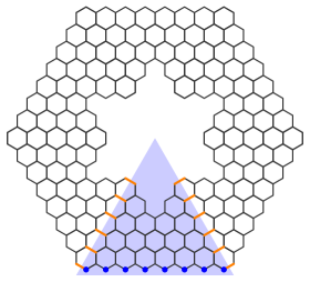
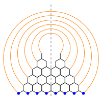
Figure 2: On the left the hexagonal graph corresponding to a $PCSSCPP$. The number of orange edges is $2n-k$ , while the number of boundary vertices on the bottom side is $2n$. The shaded region is a fundamental domain. On the right is the graph $G(n,k)$ obtained by restricting to the fundamental domain and making the identifications of the orange edges imposed by the cyclic symmetry.

Thanks to the symmetry under a rotation of $\pi/3$, it is sufficient to consider dimer coverings of the fundamental domain with “periodic boundary conditions” which are nothing else than dimer covering of a graph obtained by cutting the fundamental domain and joining the opposite cutted edges as on the right of Figure 2. Let us call $G(n,k)$ this graph. Notice that $G(n,k)$ is a planar graph symmetric under reflection along the vertical axis. In [10] Ciucu has proven that $M(G)$, the enumeration of dimer coverings of a planar graph $G$ with reflection symmetry, is related to the weighted enumerations of dimers covering of different graph $\tilde{G}$, obtained from $G$ by removing the edges incident to the symmetry axis and lying on its right (see Figure 3). The relation reads

$$M(G)=2^{r}M(\tilde{G}),$$

where $r$ is the number of edges lying on the symmetry axis, and the weighted enumeration $M(\tilde{G})$ is obtained by assigning a weight $1/2$ to each dimer lying on the symmetry axis.

In the case of PCSSCPP we are led to consider weighted dimers covering of the graph $\tilde{G}(n,k)$ reported in Figure 3, which can also be seen as Rhombus Tilings of the domain $\tilde{D}(n,k)$ or as Non-Intersecting Lattice paths starting from the right boundary of $\tilde{D}(n,k)$ and ending on its north-west boundary. This last representation allows to use the Lindström-Gessel-Viennot theorem and find

$$CSSCPP(2n,k)=2^{n-k}M(\tilde{G}(n,k))=\det[Q_{i+k,j+k}]_{1\leq i,j\leq n-k}$$ (112)

with

$$Q_{i,j}=2\binom{i+j-2}{2j-i-2}+\binom{i+j-2}{2j-i-1}$$ (113)

The determinant of $Q_{i+k,j+k}$ can be evaluated using Theorem 40 of [24] and we get

$$CSSCPP(2n,k)=\prod_{h=1}^{n-k}\frac{(j-1)!(j+2k-1)!(3j+3k-2)!(3j+3k-2)!}{(2j+k-1)!(2j+k-2)!(2j+3k-1)!(2j+3k-2)!}$$ (114)

from which one easily finds

$$\frac{CSSCPP(2n,k-1)}{CSSCPP(2n,k)}=\frac{(2k-2)!(2k-1)!(2n+k-1)!(n-k)!}{(k-1)!(3k-3)!(3k-1)(2n-k)!(n+k-1)!}.$$ (115)

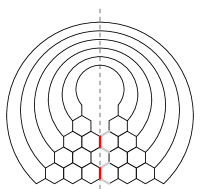
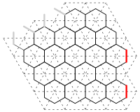
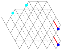
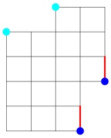
Figure 3: a) The domain $\tilde{G}(n,k)$, obtained from $\tilde{G}(n,k)$ by removing the edges incident to the symmetry axis and lying on its right. The dimers on the red edges, which lye on the symmetry axis, have weight $1/2$. b) Another presentation of the graph $\tilde{G}(n,k)$ and in dashed the corresponding domain $\tilde{D}(n,k)$. c) The domain $\tilde{D}(n,k)$. In dashed is the square lattice on which run the NILPs starting from the blue points and ending on the cyan points. d) A redrawing of the the square lattice of the NILPs. Each path going through a red edge gets a weight $1/2$.

References

• [1] R.J. Baxter, Exactly solved models in statistical mechanics (London: Academic; New York: Dover).
• [2] E. Barouch and B. M. McCoy, Phys. Rev. A 3, 786 (1971)
• [3] A. V. Razumov, Yu. G. Stroganov, J.Phys. A34 (2001) 3185, arXiv:cond-mat/0012141.
• [4] A. V. Razumov, Yu. G. Stroganov, J.Phys. A34 (2001) 5335-5340, arXiv:cond-mat/0102247.
• [5] M. T. Batchelor, J. de Gier and B. Nienhuis, J. Phys. A 34 (2001) L265-L270, arXiv.org:cond-mat/0101385.
• [6] A. V. Razumov, Yu. G. Stroganov, Theor. Math. Phys. 138 (2004) 333-337; Teor. Mat. Fiz. 138 (2004) 395-400, arXiv:math.CO/0104216. A. V. Razumov, Yu. G. Stroganov, Theor. Math. Phys. 142 (2005) 237-243; Teor. Mat. Fiz. 142 (2005) 284-292, arXiv:cond-mat/0108103.
• [7] L. Cantini, A. Sportiello, J. Combin. Theory Ser. A 118 (2011), 123–146, arXiv:math/1003.3376.
• [8] P. Di Francesco, P. Zinn-Justin, E. J. Combi. 12 (1)(2005), R6, arXiv:math-ph/0410061.
• [9] P Di Francesco 2005 J. Phys. A: Math. Gen. 38 6091, arXiv:math-ph/0504032. P. Zinn-Justin, J. Stat. Mech. Theory Exp. 1 (2007), P01007, arXiv:math-ph/0610067. L. Cantini, arXiv:math-ph/0903.5050. J. de Gier, A. Ponsaing, K. Shigechi, J. Stat. Mech. 0904 (2009) P04010, arXiv:math-ph/0901.2961.
• [10] M. Ciucu, J. Comb. Theory Ser. A 77 (1997), 67–97,
• [11] P. Di Francesco, P. Zinn-Justin, J.-B. Zuber, J. Stat. Mech. (2006) P08011, arXiv:math-ph/0603009.
• [12] N. Kitanine, J.M. Maillet, N.A. Slavnov, V. Terras, J.Phys. A35 (2002) L385-L391, arXiv:hep-th/0201134.
• [13] P. Di Francesco, P. Zinn-Justin, Comm. Math. Phys. 262 (2) (2006), 459-487, arXiv:math-ph/0412031. P. Zinn-Justin, Comm. Math. Phys. 272 (3) (2007), 661-682, arXiv:math-ph/0603018. L. Cantini J. Stat. Mech. (2007),08, P08012-P08012, arXiv:math-ph/0703087.
• [14] V. Pasquier, Ann. Henri Poincare, vol. 7, (3), (2006), 397-421, arXiv:cond-mat/0506075.
• [15] P. Di Francesco, P. Zinn-Justin, J. Phys. A 38 (2005) L815-L822, arXiv:math-ph/0508059.
• [16] I.B. Frenkel and N. Reshetikhin, Commun. Math. Phys. 146 (1992), 1–60.
• [17] A. Razumov, Yu. Stroganov and P. Zinn-Justin, J. Phys. A 40 (39) (2007), 11827-11847, arXiv:0704.3542.
• [18] P. Di Francesco and P. Zinn-Justin, Theor. Math. Phys. 154 (3) (2008), 331-348, arXiv:math-ph/070315.
• [19] P. Biane, L. Cantini, A. Sportiello, arXiv:1101.3427.
• [20] M.T. Batchelor, J. de Gier, B. Nienhuis, J.Phys.A 34 (2001) L265-L270, arXiv:cond-mat/0101385.
• [21] P. Zinn-Justin, Comm. Math. Phys. 272 (3) (2007), 661, arXiv:math-ph/0603018.
• [22] P. Di Francesco, P. Zinn-Justin, J. Phys. A 38 (48) (2005), L815-L822. arXiv:math-ph/0508059.
• [23] V. V. Bazhanov, V. V. Mangazeev, J. Phys. A: Math. Gen. 38 (2005) L145–L153. V. Bazhanov, V. V. Mangazeev, J. Phys. A: Math. Gen. 39 (2006) 12235, arXiv:hep-th/0602122. V. V. Mangazeev, V. V. Bazhanov, J. Phys. A: Math. Theor. 43 (2010) 085206, arXiv:0912.2163. A. V. Razumov and Y. G. Stroganov, Theor. Math. Phys. 164 (2010) 977–991, arXiv:0911.5030. P. Fendley and C. Hagendorf, J. Phys. A: Math. Theor. 43 (2010) 402004. C. Hagendorf, P. Fendley, arXiv:1109.4090.
• [24] C. Krattenthaler, Séminaire Lotharingien Combin. 42 (1999) (“The Andrews Festschrift”), B42q, arXiv:math/9902004.