Explicit solutions for effective four- and five-loop QCD running coupling

Abstract

We start with the explicit solution, in terms of the Lambert $W$ function, of the renormalization group equation (RGE) for the gauge coupling in the supersymmetric Yang-Mills theory described by the well-known NSVZ $\beta$-function. We then construct a class of $\beta$-functions for which the RGE can be solved in terms of the Lambert $W$ function. These $\beta$-functions are expressed in terms of a function which is a truncated Laurent series in the inverse $u$ of the gauge coupling $a\equiv\alpha/\pi$. The parameters in the Laurent series can be adjusted so that the first coefficients of the Taylor expansion of the $\beta$-function in the gauge coupling $a$ reproduce the four-loop or five-loop QCD (or SQCD) $\beta$-function.
Keywords: Exact RGE solution, Lambert function, Cardano equation

I Introduction

QCD running coupling $a(Q^{2})$ in QCD is defined as $a(Q^{2})\equiv\alpha_{S}(Q^{2})/\pi\equiv g^{2}(Q^{2})/4\pi^{2}$ where $\alpha_{S}(Q^{2})$ is the strong coupling parameter. It is the solution of the renormalization group equation (RGE)

$$\frac{da}{d\log Q^{2}}=\beta(a)\equiv-\beta_{0}a^{2}-\beta_{1}a^{3}-\beta_{2}a^{4}-\cdots\ ,$$ (1)

in which the coefficients $\beta_{0}$ and $\beta_{1}$ are universal ($\beta_{0}=(11-2n_{f}/3)/4$, $\beta_{1}=(102-38n_{f}/3)/16$), and $\beta_{j}$ ($j\geq 2$) characterize the chosen renormalization scheme (RSch). In this paper we use the notation $t=\log(Q^{2}/\Lambda^{2})$ and $c_{j}=\beta_{j}/\beta_{0}$ and the previous equation becomes

$$\frac{da}{dt}=\beta(a)\equiv-\beta_{0}a^{2}(1+c_{1}a+c_{2}a^{2}+c_{3}a^{3}+\cdots)\ .$$ (2)

The analytic structure of the running coupling in the complex $Q^{2}$ plane that corresponds to the $\beta$-function of the type

$$\beta(a) = -\beta_{0}a^{2}\frac{1+(c_{1}-c_{2}/c_{1})a}{1-(c_{2}/c_{1})a}$$ (3)

$$= -\beta_{0}a^{2}\left(1+c_{1}a+c_{2}a^{2}+(c_{2}^{2}/c_{1})a^{3}+(c_{2}^{3}/c_{1}^{2})a^{4}+\cdots\right)$$ (4)

has been investigated thoroughly in ref. Gardi:1998qr . The solution has been reduced to Lambert function W, that allowed the authors of ref. Gardi:1998qr to study the cuts of analytic continuation in the complex plane at the effective three-loop level. By choosing the value of the coefficient $c_{2}$ in the $\beta$-function (3) accordingly, this $\beta$-function can agree with any chosen $\beta$-function up to the three-loop level, as seen from the expansion eq. (4). Thus, up to the three-loop level, the exact solution of ref. Gardi:1998qr can be used as the running coupling $a(Q^{2})$. The latter depends, in addition, on the given initial condition or, equivalently, on the QCD scale $\Lambda$).

In this paper we extend the effective three-loop solution of ref. Gardi:1998qr for the running coupling to the effective four-loop and five-loop solutions. We further show that the scale $\Lambda$ always enters in the result as an argument of the Lambert function. In section II we present the exact solution to the RGE of the NSVZ $\beta$-function Novikov:1983uc , in terms of the Lambert $W$ function. In section III we propose an ansatz for a class of $\beta$-functions that generalizes the NSVZ $\beta$-function Novikov:1983uc . In sections IV and V we present solutions to the RGE’s of this class of $\beta$-functions, for the cases when the Taylor expansion reproduces the (arbitrarily chosen) coefficients of the four- and five-loop $\beta$-functions, respectively. We show that the RGE’s of such class of $\beta$-functions have solutions in terms of the Lambert $W$ function. Further, we show that solving the RGE’s of this class of the effective four- and five-loop $\beta$-functions reduces to finding the roots of a quadratic or cubic equation, respectively. In the case of the effective four-loop solution (for $c_{3}\geq 0$), we present in subsection IV.4 detailed numerical results of the evaluations of our formulas, for the ${\overline{\rm MS}}$ RSch choice of $c_{2}$ and $c_{3}$ coefficients (with $n_{f}=3$). In section VI we present the conclusions.

II NSVZ $\beta$-function

The NSVZ $\beta$-function has been found from instanton calculus and for ${\cal N}=1$ supersymmetric Yang-Mills theory takes the form Novikov:1983uc

$$\beta_{\alpha}=-\frac{\alpha^{2}}{4\pi}\frac{3N}{1-\frac{N}{2\pi}\alpha},$$ (5)

where $\alpha=g^{2}/4\pi$ and the gauge group is $SU(N)$. The number of colors is $N.$ This model is called supersymmetric QCD (SQCD). This result does not suppose that there are any flavors in the theory, that is the theory includes gluons and their superpartners gluinos. At present, this is the only nontrivial $\beta$-function known in all the number of loops.

Initially, the $\beta$-function (5) has been found in the second entry of Ref. Novikov:1983uc . The construction in that paper has been based on the fact that in supersymmetric Yang-Mills theory the axial anomaly, the anomaly of the trace of the energy-momentum tensor and the supersymmetry anomaly form the components of a supermultiplet. The divergence of the axial current is one of two terms of a component of the supermultiplet. Another term of the same component is proportional to the right-hand side of the relation for the axial anomaly. The coefficient of proportionality between the divergence of the axial current and the component of the supermultiplet can be interpreted as a $\beta$-function and coincides with NSVZ $\beta$-function (5) found later in Ref. Novikov:1983uc , first entry.

In our notation ($a\equiv\alpha/\pi$) the NSVZ $\beta$-function takes the form:

$$\frac{da}{dt}=\beta(a)\equiv-\frac{a^{2}}{4}\frac{3N}{1-\frac{N}{2}a}.$$ (6)

Eq. (6) is an ordinary differential equation of the first order and can be solved in terms of the Lambert ${\rm W}$ function. Since we will need, in the next sections, to use the procedure of deriving the solution, we write the procedure in detail.

The chain of transformations is

$$\frac{da}{dt}=a^{\prime}=-\frac{a^{2}}{4}\frac{3N}{1-\frac{N}{2}a}\Rightarrow-\frac{a^{\prime}}{a^{2}}=\frac{1}{4}\frac{3N}{1-\frac{N}{2}a}\Rightarrow$$

$$\left(\frac{1}{a}\right)^{\prime}=\frac{1}{4}\frac{3N}{1-\frac{N}{2}a}\Rightarrow\left(\frac{2}{Na}\right)^{\prime}=\frac{3/2}{1-\frac{Na}{2}}\Rightarrow u^{\prime}=\frac{3/2}{1-1/u},$$

where the substitution $u(t)=2/(Na(t))$ is done. The solution of the last equation can be found in the following way:

$$u^{\prime}=\frac{3/2}{1-1/u}\Rightarrow u^{\prime}(1-1/u)=3/2\Rightarrow(u-\ln u)^{\prime}=3/2$$

$$\Rightarrow u-\ln u=\frac{3}{2}t+C\Rightarrow e^{u}/u=e^{\frac{3}{2}t+C}\Rightarrow-\frac{1}{We^{W}}=e^{\frac{3}{2}t+C},$$

where $W=-u$ and $C$ is a constant. As a result we obtain

$$We^{W}=-e^{-\frac{3}{2}t-C}\equiv z.$$ (7)

Equation $We^{W}=z$ defines the Lambert $W$ function for the inverse relation $W=W(z).$ Taking into account all the previous steps, the solution to the NSVZ equation is

$$u(t) = -W\left(-e^{-\frac{3}{2}t-C}\right)$$

$$\Rightarrow a(t)=\frac{2}{Nu(t)} = -\frac{2}{N}\frac{1}{W\left(-e^{-\frac{3}{2}t-C}\right)}.$$ (8)

To interpret this result physically, one needs to analyze the inverse relation $W=W(z)$ of the relation $We^{W}=z(W).$ The function $z(W)$ has a minimum at the point $W=-1$ equal to $-1/e.$ The derivative $z^{\prime}(W)$ at this point is zero (see Fig. 1(a)) and this is the branching point for the analytic continuation of the inverse function $W(z)$ to the complex plane. Let’s consider first only the real values of the argument $z$ of function $W(z)$. In order to construct the inverse function $W(z)$, we should choose between the part of ${\mathbb{R}}$ to the left of the minimum and the part of ${\mathbb{R}}$ to the right of the minimum, since we need to have one-to-one correspondence between the argument and the function for any given interval.

To make this choice, we impose the physical requirements, such as positivity, reality, continuity, and the asymptotic freedom for the running coupling parameter $a(t)$ in eq. (8). The interval of $W\in~{}]-\infty,-1]$ fits these criteria, because $W$ is negative in that interval ($a(Q^{2})$ is positive). Moreover, when $W\rightarrow-\infty$, we have $z\rightarrow 0^{-},$ $a(Q^{2})\rightarrow 0^{+}$, and this represents the asymptotic freedom of the coupling constant $a(Q^{2})$.

The interval to the right of the minimum, $W\in~{}[-1,\infty[$, does not fit most of these criteria, since the coupling constant becomes discontinuous (infinite) at the point $W=0,z=0$.

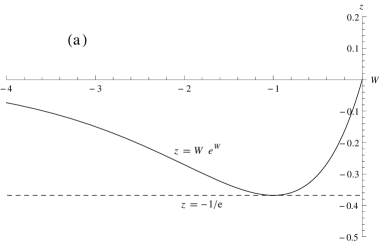
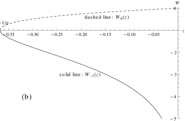
Figure 1: (a) The inverse Lambert relation $z=We^{W}$, for negative $W$ (where $z$ is negative, i.e., $Q^{2}$ positive); (b) The Lambert function $W=W(z)$ at negative $z$ ($-1/e<z<0$) - two branches are presented: $W_{-1}(z)$ and $W_{0}(z)$. We see that for $z\to-0$ (i.e., $Q^{2}\to+\infty$), $W_{-1}(z)\to-\infty$ and $W_{0}(z)\to 0$.

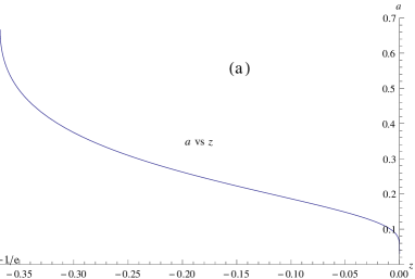
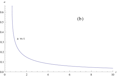
Figure 2: (a) Coupling $a$ of Eq. (8), with $W_{-1}$ (and $N=3$), as a function of negative $z$ ($-1/e<z<0$); (b) $a$ as a function of $t=-(2/3)\ln(-z)=\ln(Q^{2}/\Lambda^{2})$, for $2/3<t<\infty$, corresponding to $-1/e<z<0$. The scale $\Lambda^{2}$ is such that $C=0$, cf. also Eq. (9). At $t=2/3$ (i.e., $Q^{2}=\Lambda^{2}e^{2/3}$) a Landau singularity appears, the value of $a$ there is $2/N$ ($=2/3$).

Thus, we have to choose the interval of $W\in~{}]-\infty,-1]$, i.e., the branch $W_{-1}$ of the Lambert function - see also Figs. 1 and 2. The value of $z$ in this interval is changing between $z(-1)=-1/e$ and $z(-\infty)=0^{-}.$ The variable $z$ defined by eq. (7) is related to the momentum transfer $Q^{2}$ as

$$z=-e^{-\frac{3}{2}t-C}=-\left(\frac{Q^{2}}{\Lambda^{2}}\right)^{-3/2}=-\left(\frac{\Lambda^{2}}{Q^{2}}\right)^{3/2}\ ,$$ (9)

where $\Lambda$ is an arbitrary scale. Arbitrariness of this scale follows from the definition of $t=\ln(Q^{2}/M^{2})$, where $M^{2}$ is the Pauli-Villars regulator in the work of ref. Novikov:1983uc . An arbitrary constant $C$ of eq. (9) is typical for differential equation and it has been absorbed in $M^{2}$ to create the scale $\Lambda^{2}$ in eq. (9). In QCD, the scale $\Lambda$ is identified with a specific physical scale, but this is not the case here since this model does not have any physical scale at which the coupling parameter $a(t)$ is measured. Equation (9) is an explicit relation between $z$ and $Q^{2},$ namely $z=-1/e$ corresponds to $Q^{2}=\Lambda^{2}e^{2/3}$ and $z=0^{-}$ corresponds to $Q^{2}\rightarrow\infty.$

The physical solution, eq. (8), can be written as

$$a(Q^{2})=-\frac{2}{N}\frac{1}{W_{\mp 1}\left(-(\Lambda^{2}/Q^{2})^{3/2}\right)}\ ,$$ (10)

where the branch $W_{-1}$ is taken for all $Q^{2}$ with ${\rm Im}Q^{2}\geq 0$, and $W_{+1}$ when ${\rm Im}Q^{2}<0$. Analytic structure of this function in the complex $Q^{2}$ plane has a cut for $Q^{2}\in~{}]-\infty,Q_{b}^{2}]$ where $Q_{b}^{2}\equiv\Lambda^{2}\exp(2/3)$ ($>0$) is the branching point. The cut of $a(Q^{2})$ on the positive $Q^{2}$ semiaxis is not physical, in the sense that it does not respect the analytic properties of the spacelike observables ${\cal D}(a(Q^{2}))$. The latter properties are dictated by the locality and causality of quantum field theories BS ; Oehme .. The NSVZ $\beta$-function leads to an $a(Q^{2})$, Eq. (10), with a cut on the positive axis $Q^{2}\in~{}]0,Q_{b}^{2}]$. At the branching point $Q_{b}^{2}\equiv\Lambda^{2}\exp(2/3)$ it is finite

$$a(Q_{b}^{2}\equiv\Lambda^{2}e^{2/3})=\frac{2}{N},$$ (11)

but the derivatives of this function are singular at the branching point. The maximum value of the coupling is obtained at the branching point $Q^{2}=Q_{b}^{2}$, and it goes down monotonically when $Q^{2}$ increases above $Q_{b}^{2}$. In the limit of large number of colors the maximum value of the coupling parameter goes to zero and the theory becomes a theory without interaction. If $\Lambda$ is considered to be an arbitrary unfixed scale, the branching point can be taken as close to $Q^{2}=0$ as we wish. On the other hand, if we fix $a(Q^{2})$ to a specific “initial” value at a specific value of $Q_{\rm in}^{2}$, then $\Lambda$ is fixed as well.

Below the scale $Q_{b}^{2}=\Lambda^{2}\exp(2/3)$, the NSVZ model cannot be applied, in the sense that the effective vertices (proper multipoint Green function) and effective propagators (full two-point Green function) do not exist below that scale since the running coupling “does not exist” in that region. A physical explanation for this phenomenon could be that the scattering processes in this model do not take place in that region of the low momentum transfer $Q^{2}<Q_{b}^{2}$. Any experimental confirmation of the found behavior is impossible since the model does not contain the physical particles of the Standard Model. In QCD the situation is different since the scattering takes place at any momentum transfer $Q^{2}$ (even very small). Theoretically, the corresponding positive part of the cut of $a(Q^{2})$ in the complex $Q^{2}$-plane in perturbative QCD appears as an artifact, because an approximate (truncated series) $\beta$-function is used there; and the mentioned cut is removed by the analytization procedure.

III Ansatz

The result in the previous section is not new (however, may have never been presented in such a form). As we have mentioned in the Introduction, a similar type of the $\beta$-function has been analyzed in ref. Gardi:1998qr in the context of investigation of the analyticity properties of the running coupling in the complex $Q^{2}$ plane. The explicit solution to that RGE has been found there. However, in the previous section we did not follow step-by-step the derivation of ref. Gardi:1998qr . Now we construct an ansatz for solving the RGE based on a simple generalization of the procedure described in the previous section.

As the first step, we modify eq. (8)

$$f(u(t))=-W\left(-e^{-At-C}\right)$$ (12)

where $f(u)$ is an arbitrary continuous function of $u.$ Then,

$$(f(u)-\ln f(u))^{\prime}=A\Rightarrow u^{\prime}\frac{df(u)}{du}(1-1/f(u))=A$$

$$u^{\prime}=\frac{A/f_{u}^{\prime}(u)}{1-1/f(u)}.$$

The relation between $a$ and $u$ remain the same as it stands in the previous section,

$$a(t)=\frac{2}{Bu(t)},$$ (13)

where $A$ and $B$ are some constants. Thus, we obtain

$$\left(\frac{2}{Ba(t)}\right)^{\prime}=\frac{A/f_{u}^{\prime}(\frac{2}{Ba(t)})}{1-1/f(\frac{2}{Ba(t)})}\ ,$$

where we recall that $t\equiv\ln(Q^{2}/M^{2})$. As a result, the solution to the following RGE

$$\left(a(t)\right)^{\prime}=\beta(a)=-\frac{Aa^{2}}{2}\frac{B/f_{u}^{\prime}(\frac{2}{Ba(t)})}{1-1/f(\frac{2}{Ba(t)})}\ ,$$ (14)

is obtained via the formula

$$a(t)=\frac{2}{B}\frac{1}{F(-W(e^{-At-C}))}\ ,$$ (15)

where $F$ is the inverse of the function $f$ appearing in eq. (12), i.e., $F(f(u))=u$.

The function $f(u)$ can be chosen arbitrarily. For our purpose, the ansatz will be a truncated Laurent series in $u$ with the leading term to be $u$

$$f(u)=u+a_{0}+\frac{a_{1}}{u}+\cdots+\frac{a_{n}}{u^{n}}\ .$$ (16)

In this work we will consider two ansätze for this function, one with $n=1$ and the other with $n=2$. The first one represents a beta function with four real parameters ($A$, $B$, $a_{0}$, $a_{1}$), which can be adjusted so that the expansion of $\beta(a)$ in powers of $a$ reproduces the four-loop $\beta$-function in a given renormalization scheme (RSch), i.e., the given coefficients $\beta_{0}$ and $c_{j}$ ($j=1,2,3$) of the expansion (2). The second one has five real parameters, which can be adjusted to reproduce the five-loop $\beta$-function in a given RSch. We will call the first and the second ansatz the “effective four-loop” and the “effective five-loop” $\beta$-function, respectively. As we will see in the next sections, the problem of solving these RGE’s is reduced to finding the inverse function of the function $f(u)$. This means, in practice, finding the roots of polynomials.

IV Effective four-loop case

IV.1 Four-loop ansatz for $f(u)$

We take $f(u)$ in the form

$$f(u)=u+a_{0}+\frac{a_{1}}{u}\ ,$$ (17)

where $a_{0},$ $a_{1}$ are arbitrary real numbers. We show how to reproduce the $\beta$-function up to $\sim a^{5}$ tuning these two numbers (and the numbers $A$ and $B$)

$$\beta(a)=-\beta_{0}a^{2}~{}(1+c_{1}a+c_{2}a^{2}+c_{3}a^{3})+{\cal O}(a^{6})\ .$$

We note that $\beta_{0}$ and $c_{1}$ are universal in mass-independent schemes, and $c_{j}$ ($j\geq 2$) are the parameters which characterize RSch. Thus, we consider the $\beta$-function as determined in the previous section

$$\beta(a)=-\frac{Aa^{2}}{2}\frac{B/f_{u}^{\prime}(u)}{1-1/f(u)},$$ (18)

where $f(u)$ is given in eq. (17). We conclude that

$$\beta_{0}=\frac{AB}{2}.$$ (19)

With the coefficient $B$ fixed, we choose $A$ to adjust $\beta_{0}$. Now we show how to fix the coefficient $B.$ In the fraction

$$\frac{1/f_{u}^{\prime}(u)}{1-1/f(u)},$$ (20)

we change temporarily the normalization of $a$ in order to simplify the calculation, $u=1/a$, since $a$ appears only with the factor $2/B$. The correct normalization will be recovered afterwards, by a simple redefinition of $a$,

$$u=2/(Ba)\ .$$ (21)

Then we have

$$f_{u}^{\prime}(u)=1-\frac{a_{1}}{u^{2}}~{}~{}~{}\Rightarrow~{}~{}~{}f_{u}^{\prime}(1/a)=1-a_{1}a^{2},$$

$$f(u)=u+a_{0}+\frac{a_{1}}{u}~{}~{}~{}\Rightarrow~{}~{}~{}f(1/a)=\frac{1}{a}+a_{0}+a_{1}a,$$

$$1/f_{u}^{\prime}(1/a)=\frac{1}{1-a_{1}a^{2}}=1+a_{1}a^{2}+{\cal O}(a^{4})\ .$$

Then, the expansion can be performed directly and we obtain

$$\frac{1/f_{u}^{\prime}(1/a)}{1-1/f(1/a)}=1+a+(a_{1}-a_{0}+1)a^{2}+(a_{0}-1)^{2}a^{3}+{\cal O}(a^{4})\ .$$

We now restore the original normalization for the running coupling $a$, eq. (21), and require the $\beta$-function to be in a given RSch up to four loops

$$1+Ba/2+(a_{1}-a_{0}+1)(Ba/2)^{2}+(a_{0}-1)^{2}(Ba/2)^{3}=1+c_{1}a+c_{2}a^{2}+c_{3}a^{3}.$$

Thus, we deduce

$$B/2=c_{1}\ ,\quad(a_{1}-a_{0}+1)(B/2)^{2}=c_{2}\ ,\quad(a_{0}-1)^{2}(B/2)^{3}=c_{3}\ .$$ (22)

The first identity determines $B=2c_{1}$. The other two identities then take the following form:

$$a_{1}-a_{0}+1=c_{2}/c_{1}^{2} \equiv \omega_{1}\ ,\quad(a_{0}-1)^{2}=c_{3}/c_{1}^{3}\equiv\omega_{2}\ .$$ (23)

The solution is

$$a_{0}^{(\pm)} = \pm\sqrt{\omega_{2}}+1=\pm\sqrt{c_{3}/c_{1}^{3}}+1\ ,$$

$$a_{1}^{(\pm)} = \omega_{1}\pm\sqrt{\omega_{2}}=(c_{2}/c_{1}^{2})\pm\sqrt{c_{3}/c_{1}^{3}}\ .$$ (24)

We have to assume that $\omega_{2}\geq 0$, because otherwise our ansatz would give us a $\beta$-function with nonreal coefficients.

IV.2 The inverse function of $f(u)$

Knowing explicitly the coefficient $a_{0},$ $a_{1}$ in the ansatz (17)

$$-W=u+a_{0}+\frac{a_{1}}{u},$$ (25)

we rewrite it in the form

$$u^{2}+(a_{0}+W)u+a_{1}=0,$$

that is in its turn a usual quadratic equation. Taking into account the result for the previous subsection, the equation takes the form

$$u^{2}+(\pm\sqrt{\omega_{2}}+1+W)u+\omega_{1}\pm\sqrt{\omega_{2}}=0.$$

The two roots for this equation are

$$u_{1,2}=\frac{-(\pm\sqrt{\omega_{2}}+1+W)\pm\sqrt{(\pm\sqrt{\omega_{2}}+1+W)^{2}-4(\omega_{1}\pm\sqrt{\omega_{2}})}}{2}.$$ (26)

IV.3 Cut structure and analyticity

We first analyze eq. (26) for the real value of the argument $z$ of the Lambert function $W(z)$. The variable $z$ defined by eq. (7) is related to the momentum transfer $Q^{2}$ as

$$z=-e^{-At-C}=-\left(\frac{Q^{2}}{\Lambda^{2}}\right)^{-A}=-\left(\frac{\Lambda^{2}}{Q^{2}}\right)^{A}=-\left(\frac{\Lambda^{2}}{Q^{2}}\right)^{\beta_{0}/c_{1}}\ ,$$ (27)

where $\Lambda$ is an arbitrary scale. We recall that $t\equiv\ln(Q^{2}/M^{2})$, and the arbitrary constant $C$ has been absorbed in $\Lambda^{2}$. We will assume throughout that $\beta_{0}>0$ and $c_{1}>0$.

As we mentioned earlier, the function $z(W)$ has a minimum at the point $W=-1$ equal to $-1/e.$ The derivative $z^{\prime}(W)$ at this point is zero and this is the branching point for the analytic continuation of the inverse function $W(z)$. This point remains a branching point for the function $u(t)$ found in eq. (26).

To make the choice between the part of ${\mathbb{R}}$ to the left of the minimum and the part of ${\mathbb{R}}$ to the right of the minimum, we impose, as in the NSVZ case of section II, the physical requirements: positivity, reality, continuity and asymptotic freedom for the running coupling $a(t)$ of eq. (21). The interval of $W\in~{}]-\infty,-1]$ fits these criteria under some restrictions on the relation between the coefficients $\omega_{1}$ and $\omega_{2}$. When $Q^{2}\to\infty$, we have $z\to 0^{-}$, and $W\to-\infty$; the asymptotic freedom of $a(Q^{2})$ then implies that we must have the positive sign in front of the square root in eq. (26)

$$u\left(=\frac{1}{c_{1}a}\right)=\frac{-(\pm\sqrt{\omega_{2}}+1+W)+\sqrt{(\pm\sqrt{\omega_{2}}+1+W)^{2}-4(\omega_{1}\pm\sqrt{\omega_{2}})}}{2}.$$ (28)

The interval to the right of the minimum, which is $W\in~{}[-1,\infty[$, does not fit these physical criteria, for the same reasons as in the NSVZ case. In particular, when $z\to 0^{-}$, this branch gives $W\to 0^{-}$, contravening the asymptotic freedom.

Therefore, we have to choose the interval of $W\in~{}]-\infty,-1]$, with the values of $z$ between $z(-1)=-1/e$ and $z(-\infty)=0^{-}$. This means that, if $0<\beta_{0}/c_{1}<2$, as in the NSVZ case of section II, we have to choose the branch $W_{-1}$ for the Lambert function for real $z\in(-1/e,0)$, i.e., for $Q^{2}\in(Q_{b}^{2},+\infty)$ where $Q_{b}^{2}\equiv\Lambda^{2}\exp(c_{1}/\beta_{0})$. For details on this point, we refer to the later analysis of the continuation of $a(Q^{2})$ to complex $Q^{2}$, later in this subsection.

The solution of the RGE (14) can now be written as

$$a(Q^{2})=-\frac{2}{c_{1}}\frac{1}{(\pm\sqrt{\omega_{2}}+1+W)-\sqrt{(\pm\sqrt{\omega_{2}}+1+W)^{2}-4(\omega_{1}\pm\sqrt{\omega_{2}})}}.$$ (29)

Two signs are possible, coming from eq. (24), and we will consider both options. In both the cases the coupling $a(Q^{2})$ goes down monotonically to zero with increasing $Q^{2}$. Monotonic behavior can be checked directly from (29) by taking the derivative, or by using the relation for derivative of the inverse function $u^{\prime}(W)=1/W^{\prime}(u).$

Let us choose first the lower sign in eq. (29). Provided that

$$\omega_{2}-4(\omega_{1}-\sqrt{\omega_{2}})>0\ ,$$ (30)

the branching point of $a(Q^{2})$ is at $Q_{b}^{2}\equiv\Lambda^{2}\exp(c_{1}/\beta_{0})$, and the coupling reaches there its finite maximum

$$a(Q^{2}=\Lambda^{2}e^{c_{1}/\beta_{0}})=\frac{2}{c_{1}}\frac{1}{\sqrt{\omega_{2}}+\sqrt{\omega_{2}-4(\omega_{1}-\sqrt{\omega_{2}})}}\ ,$$

but the derivatives of this function are singular there. Thus, for the choice of the lower sign the solution to RGE (14) that reproduces first four coefficients of the $\beta$-function is

$$a(Q^{2})=\frac{2}{c_{1}}\Biggl{[}\sqrt{\omega_{2}}-1-W\left(-\left(\Lambda^{2}/Q^{2}\right)^{\beta_{0}/c_{1}}\right)\Biggr{.}$$

$$\Biggl{.}+~{}~{}\sqrt{\left(\sqrt{\omega_{2}}-1-W\left(-\left(\Lambda^{2}/Q^{2}\right)^{\beta_{0}/c_{1}}\right)\right)^{2}-4(\omega_{1}-\sqrt{\omega_{2}})}\Biggr{]}^{-1}$$ (31)

where $Q^{2}\in~{}]\Lambda^{2}\exp(c_{1}/\beta_{0}),\infty[.$

In order to extend the function (31) to all the plane of complex $Q^{2}$, we need to take into account for the analytic structure of the multivalued function $W(z)$ of complex variable $z$, which is described in ref. Corless:1996zz . As it was done in ref. Gardi:1998qr , we follow ref. Corless:1996zz for the division of the branches and also for the notation. Since $W(z)$ is a multivalued function of the variable $z$, the corresponding $z$-plane has to be split in a multisheet Riemann surface with a cut for each sheet of the surface, while the complex plane of $W$ should be divided in partitions having common borders. Each partition in $W$-plane can be bijectively mapped onto one of the sheets of the Riemann surface of variable $z$. The borders of each partition transform under this map to edges of the cuts. The partitions (branches) are named $W_{0},$ $W_{1},$ $W_{-1},$ $W_{2},$ $W_{-2},$ etc. The branches $W_{n}$ with $n<0$ have negative imaginary parts, and those with $n>0$ have positive imaginary parts. The $W_{0}$ is an exceptional case, it is the only partition that contains the positive part of the real axis of the $W$-plane completely. The border of the $W_{0}$ partition can be mapped to the edges of cut $z\in]-\infty,-1/e]$, and the branching point is $z=-1/e$. The branch choices conform to the rule of counter-clockwise continuity around the branching point. This means, for example, that the upper edge of the cut $z\in]-\infty,-1/e]$ can be mapped onto the upper border of the $W_{0}$ partition in the $W$-plane. The next sheet of the Riemann surface has a double cut, one is the same $z\in]-\infty,-1/e],$ and the other is $z\in]-\infty,0]$. The first cut corresponds to the border between $W_{0}$ and $W_{\pm 1}$ partitions, and the second cut $z\in]-\infty,0]$ corresponds to the border between $W_{\pm 1}$ and $W_{\pm 2}$ partitions. According to the rule of the counter-clockwise continuity, the upper part of the cut $z\in]-1/e,0]$ transforms to the border of the $W_{-1}$ partition. This means that $W_{0}$ and $W_{-1}$ are the only partitions that contain the real values of $W$. The part of the cut $z\in]-1/e,0]$ corresponds to the border between the $W_{1}$ and $W_{-1}$ partitions. These two partitions have common real limit along $z\in]-1/e,0].$

To relate behavior of the running coupling in the complex $z$-plane and the complex $Q^{2}$-plane, the phase analysis is important. Here we mainly follow the lines of ref. Gardi:1998qr , and write the same notation $Q^{2}=|Q^{2}|e^{i\phi}$, where $-\pi<\phi<\pi$ and $z=|z|e^{i\delta}.$ We consider the case $c_{1}>0$.

The domain for the argument $z$ of the Lambert function $W(z)$ is a Riemann surface, it looks like a “pie” with many horizontal “layers”. This is in close analogy with the Riemann surface for the usual logarithmic function of the complex variable. This analogy is not surprising since for the large values of $z$ the Lambert function $W(z)$ has a logarithmic asymptotic behavior. The partitions in the $W$-plane resemble the partitions for the complex plane of the logarithmic function.

Each sheet has a cut. Each cut has two edges, and one of the edges belongs to the sheet. The edges are mapped to the borders of the partitions in the $W$-plane. The edge that belongs to the sheet should be glued to the next upper sheet (the edge does not belong to the latter). The edge that does not belong to the sheet should be glued to the edge of the previous lower sheet (the edge belongs to the latter). All this is in complete analogy with the Riemann surface for the argument of the logarithmic function.

The sheet of the surface with $-\pi<\delta\leq\pi$ is the domain of $z$ for the $W_{0}$ partition, while for $\pi<\delta\leq 3\pi$ we pass to the next domain of $z$ for the $W_{1}$ partition, and so on, encountering new domain each time the phase $\delta$ of $z$ increases by $2\pi$. Similarly, the sheet with $-3\pi<\delta\leq-\pi$ is the domain of $z$ for the $W_{-1}$ partition, and so on.

As has been done in ref. Gardi:1998qr we consider the case $c_{1}>\beta_{0}/2>0$, which is the case valid in QCD (with $0\leq n_{f}\leq 6$). As mentioned earlier, the relevant partition (branch) is $W_{-1}(z)$, and the domain of $z=|z|e^{i\delta}$ is with the phase $-3\pi<\delta\leq-\pi$. For positive $\phi$ (where $Q^{2}=|Q^{2}|e^{i\phi}$) we obtain $\delta=-\pi-(\beta_{0}/c_{1})\phi$, in accordance with eq. (27). It never reaches $W_{-1}$ partition border at $\delta=-3\pi$, since $\beta_{0}/c_{1}<2$. Similarly, for negative $\phi$ the variable $z$ is in the domain of the partition of $W_{1}(z)$ with the phase $\pi<\delta\leq 3\pi$ and we obtain $\delta=+\pi-(\beta_{0}/c_{1})\phi$. In turn, it never reaches the border of $W_{1}$ partition at $\delta=3\pi$. The only singularity that appears for the union of these partitions $W_{\mp 1}$ is the singularity at the point of the cut start, $z=-1/e,$ that corresponds to a singularity on the positive real $Q^{2}$ axis, at $Q^{2}=Q_{b}^{2}\equiv\Lambda^{2}\exp(c_{1}/\beta_{0})$.

The partitions $W_{\mp 1}(z)$ defined in the domains described above have the common continuous limit along the line $z\in]-1/e,0]$. On the other hand, this is not the only definition of the domain for the union of these partitions with the common limit along the line $z\in]-1/e,0]$. In ref. Gardi:1998qr the phase $\delta$ of $z$ is required to be in the range $-\pi<\delta\leq\pi$. If the variable $z$ is required to be in this domain, then for $c_{1}>\beta_{0}/2$ we should choose for $\phi\geq 0$ (when the partition is $W_{-1}(z)$) the phase of $z$ equal to $\delta=+\pi-(\beta_{0}/c_{1})\phi$, and for $\phi<0$ (when the partition is $W_{1}(z)$) the phase $\delta=-\pi-(\beta_{0}/c_{1})\phi$. In both cases it never reaches the borders of the partitions, which is $\delta=-\pi$ for $W_{-1}$ and $\delta=\pi$ for $W_{1}$. In contrast, if we had $\beta_{0}/2>c_{1}>0$, then $\delta=\pm\pi-(\beta_{0}/c_{1})\,\phi$ and the border of the partitions $W_{\pm 1}(z)$ would be reached at the value of the phase $\phi$ of $Q^{2}$: $\phi=\pm 2(c_{1}/\beta_{0})\pi$. At this point we would have to include the neighboring partitions, increasing the modulo of their index by one, i.e., in such a case it would be $W_{\pm 2}.$

Analytic structure of the aforementioned function $W_{\mp 1}(z)$ in the complex $Q^{2}$ plane has a cut for $]-\infty,\Lambda^{2}\exp(c_{1}/\beta_{0})]$, which contains the entire real negative axis and a part of positive axis, $]0,\Lambda^{2}\exp(c_{1}/\beta_{0})]$; the branching point for this cut is $Q_{b}^{2}=\Lambda^{2}\exp(c_{1}/\beta_{0})$ (in analytic QCD models the part of positive axis is removed by analytization procedure).

The analytic structure described in the previous paragraphs is caused by the multivaluedness of the Lambert function, since the running coupling $a(Q^{2})$ is a composite function of the Lambert function. However, the square root in eq. (31) is a multivalued function too,

$$\varphi(W)=\sqrt{\left(\sqrt{\omega_{2}}-1-W\right)^{2}-4(\omega_{1}-\sqrt{\omega_{2}})},$$ (32)

and the complex $\varphi$-plane should also be divided in partitions. Each partition can be mapped bijectively onto the corresponding partition of the $W$-plane, which in its turn is bijectively mapped onto the entire $z$-plane that has the cut described in the previous paragraphs corresponding to the borders of the $W$-partition in which we work. The cut in the $W$-partition, caused by the multivaluedness of $\varphi(W)$, starts at the point where the argument of the square root in $\varphi$ is zero,

$$\left(\sqrt{\omega_{2}}-1-W\right)^{2}\leq 4(\omega_{1}-\sqrt{\omega_{2}})~{}~{}~{}\Rightarrow$$

$$-2\sqrt{\omega_{1}-\sqrt{\omega_{2}}}\leq~{}~{}\sqrt{\omega_{2}}-1-W~{}~{}\leq 2\sqrt{\omega_{1}-\sqrt{\omega_{2}}},$$

$$-2\sqrt{\omega_{1}-\sqrt{\omega_{2}}}-\sqrt{\omega_{2}}\leq~{}~{}-1-W~{}~{}\leq 2\sqrt{\omega_{1}-\sqrt{\omega_{2}}}-\sqrt{\omega_{2}},$$

$$-1+2\sqrt{\omega_{1}-\sqrt{\omega_{2}}}+\sqrt{\omega_{2}}\geq~{}~{}W~{}~{}\geq-1-2\sqrt{\omega_{1}-\sqrt{\omega_{2}}}+\sqrt{\omega_{2}},$$ (33)

and connect these two limiting real points, $W=-1+\sqrt{\omega_{2}}-2\sqrt{\omega_{1}-\sqrt{\omega_{2}}}$ and $W=-1+\sqrt{\omega_{2}}+2\sqrt{\omega_{1}-\sqrt{\omega_{2}}}$. If $\sqrt{\omega_{2}}-2\sqrt{\omega_{1}-\sqrt{\omega_{2}}}$ is a positive real value, eq. (30), the cut is not in the physical partition of the $W$-plane corresponding to our ansatz, it is situated in the $W_{0}$ partition of the $W$-plane. Thus, the cut structure of $a(Q^{2})$, in the case of the lower sign in eqs. (24) and (29), is dictated by the cut of $W_{\mp 1}(z)$, and not by the cut of $\varphi(W(z))$, i.e., it starts at $Q_{b}^{2}=\Lambda^{2}\exp(c_{1}/\beta_{0})$.

For the choice of the upper sign in (24), the result for the running coupling is

$$a(Q^{2})=-\frac{2}{c_{1}}\frac{1}{(\sqrt{\omega_{2}}+1+W)-\sqrt{(\sqrt{\omega_{2}}+1+W)^{2}-4(\omega_{1}+\sqrt{\omega_{2}})}}.$$ (34)

In this case the analytic structure due to the Lambert function is the same as for the choice of the lower sign, but the cut due to the square root can enter the physical region. The maximal value of the running coupling in this case is reached at the left edge of the horizontal cut, entering the $W_{1}$-partition, produced by the square root function in the denominator. In the next subsection we present numerical results for evaluation of the cut structure in this case of choosing the upper sign.

IV.4 Numerical application of analytic formulas

In QCD, the first two universal coefficients $\beta_{0}$ and $\beta_{1}$ ($\equiv c_{1}\beta_{0}$) are: $\beta_{0}=(11-2n_{f}/3)/4$ and $\beta_{1}=(102-38n_{f}/3)/16$. It turns out that in QCD, for all numbers of active quark flavors ($0\leq n_{f}\leq 6$), we have $c_{1}>\beta_{0}/2$, i.e., the case described in this section (i.e., the case (c) in section 3 of ref. Gardi:1998qr ). Therefore, our formula (29) becomes relatively simple, as in the two-loop (c) case of ref. Gardi:1998qr

$$a^{(+)}(Q^{2}) = \frac{2}{c_{1}}\left[-\sqrt{\omega_{2}}-1-W_{\mp 1}(z)+\sqrt{(\sqrt{\omega_{2}}+1+W_{\mp 1}(z))^{2}-4(\omega_{1}+\sqrt{\omega_{2}})}\right]^{-1},$$ (35)

$$a^{(-)}(Q^{2}) = \frac{2}{c_{1}}\left[\sqrt{\omega_{2}}-1-W_{\mp 1}(z)+\sqrt{(\sqrt{\omega_{2}}-1-W_{\mp 1}(z))^{2}-4(\omega_{1}-\sqrt{\omega_{2}})}\right]^{-1}.$$ (36)

where $Q^{2}=|Q^{2}|\exp(i\phi)$, and the upper indices in $W$ and $z$’s in eqs. (35)-(36) are to be used when $0\leq\phi<\pi$, the lower indices when $-\pi\leq\phi<0$, and $z$ is given in eq. (27). The superscripts ’$(+)$’ and ’$(-)$’ indicate that we take the upper and the lower sign in eqs. (24) and (29), respectively. We recall that both of these solutions (35)-(36) work for any choices of real $c_{2}$ and nonnegative $c_{3}$, i.e., in a sense they are effective “four-loop” solutions of the RGE (but with coefficients $c_{4},c_{5},\ldots$ depending on our choice of $c_{2}$ and $c_{3}$). The corresponding formula for the (pure) two-loop case (i.e., with $c_{2}=c_{3}=\cdots=0$), ref. Gardi:1998qr , is

$$a^{(2-\ell)}(Q^{2})=-\frac{1}{c_{1}}\frac{1}{\left[1+W_{\mp 1}(z)\right]}\ ,$$ (37)

and the “three-loop” case of the beta function (3) is similar to the previous (ref. Gardi:1998qr )

$$a^{(3-\ell)}(Q^{2})=-\frac{1}{c_{1}}\frac{1}{\left[1-(c_{2}/c_{1}^{2})+W_{\mp 1}(z)\right]}\ .$$ (38)

In order to present the numerical results of the formulas (35) and (36), we choose the ${\overline{\rm MS}}$ renormalization scheme with $n_{f}=3$ (low energy QCD). In this case, $\beta_{0}=9/4$; $c_{1}=16/9=1.77778$; $c_{2}=3863/864=4.47106$; $c_{3}=20.9902$.

The two effective “four-loop” beta functions, eq. (18), $\beta^{(\pm)}(a)$, (i.e., for the choice of $+\sqrt{\omega_{2}}$ and $-\sqrt{\omega_{2}}$) are

$$\beta^{(\pm)}(a) = -\beta_{0}a^{2}\frac{\left[1+(a_{0}^{(\pm)}c_{1})a+(a_{1}^{(\pm)}c_{1}^{2})a^{2}\right]}{\left[1+(a_{0}^{(\pm)}-1)c_{1}a+(a_{1}^{(\pm)}c_{1}^{2})a^{2}\right]\left[1-(a_{1}^{(\pm)}c_{1}^{2})a^{2}\right]}\ ,$$ (39)

with the constants $a_{0}^{(\pm)}$ and $a_{1}^{(\pm)}$ given by eqs. (24). As argued, expansion of both beta functions agrees, up to terms $\sim a^{5}$, with the four-loop ${\overline{\rm MS}}$ beta function. The coefficients $c_{j}$ for $j\geq 4$ differ, though. For example, $c_{4}^{(+)}=104.43$ and $c_{4}^{(-)}=84.81$.

In order to fix the scales $\Lambda$ appearing in eq. (27), we have to adjust the couplings at a specific scale of reference to specific values. We take the approximate world average $a(M_{Z}^{2},{\overline{\rm MS}})\approx 0.119/\pi$, ref. PDG2008 ; PDG2010 , and RGE-run it (at four-loop) down to the reference scale $\mu^{2}_{\rm in}=(3m_{c})^{2}$ ($\approx 14.516\ {\rm GeV}^{2}$). The quark threshold matching is implemented at the three-loop level, ref. CKS , at threshold scales $Q^{2}=3m_{q}^{2}$ ($q=b,c$). We thus obtain the reference value, in ${\overline{\rm MS}}$

$$a_{\rm in}\equiv a((3m_{c})^{2};n_{f}=3)\approx 0.07245\ .$$ (40)

This is the reference value we use in all our numerical calculations, with $n_{f}=3$.

It turns out that the branching point in the complex $Q^{2}$-plane, where the unphysical (Landau) cut of $a(Q^{2})$ starts, is somewhat lower if we evaluate our formulas with $+\sqrt{\omega_{2}}$ than with $-\sqrt{\omega_{2}}$. Therefore, we present our numerical results for the case of $+\sqrt{\omega_{2}}$, i.e., formulas (35) for $a^{(+)}$ and $\beta^{(+)}$ in eq. (39).

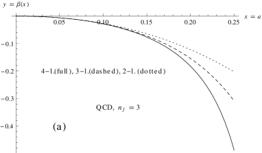
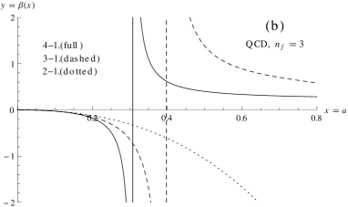
Figure 3: (a) Beta functions $\beta(a)$: the four-loop beta function $\beta^{(+)}$ eq. (39), the three-loop beta function eq. (3), and the two-loop beta function; (b) The same, for a wider scale of $a$, so that singularities are seen.

In figs. 3(a),(b), we present the beta functions $\beta(a)$, four our effective four-loop case [$\beta^{(+)}$, eq. (39)], the effective three-loop case (3), and the two-loop case.

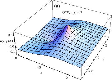
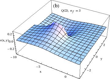
Figure 4: The (a) real and (b) imaginary part of the effective four-loop coupling $a^{(+)}(Q^{2})$, where $x=\ln(|Q^{2}|/\mu^{2}_{\rm in})$ ($\mu^{2}_{\rm in}\approx 14.516\ {\rm GeV}^{2}$) and $y={\rm Arg}(Q^{2})$.

In figs. 4(a),(b), we present the resulting real and imaginary parts of $a(Q^{2})$ for complex $Q^{2}$, in the complex plane $x+iy=\ln(Q^{2}/\mu_{\rm in}^{2})$, i.e., where $Q^{2}=\mu_{\rm in}^{2}\exp(x)\exp(iy)$, with $-\pi<y<\pi$, and $u(x,y)\equiv{\rm Re}a(Q^{2})$ and $v(x,y)={\rm Im}a(Q^{2})$. The point $x=y=0$ corresponds to $Q^{2}=\mu_{\rm in}^{2}\approx 14.516\ {\rm GeV}^{2}$; the line with $y=0$ corresponds to positive $Q^{2}$, while the lines with $y=\pm\pi$ correspond to negative $Q^{2}$. These figures clearly indicate that there is a (Landau) singularity, which starts at the (Landau) branching point $x_{b}\approx-3.170$, corresponding to the branching point $Q_{b}^{2}\approx 0.610\ {\rm GeV}^{2}$, i.e., $Q_{b}\approx 0.781$ GeV.

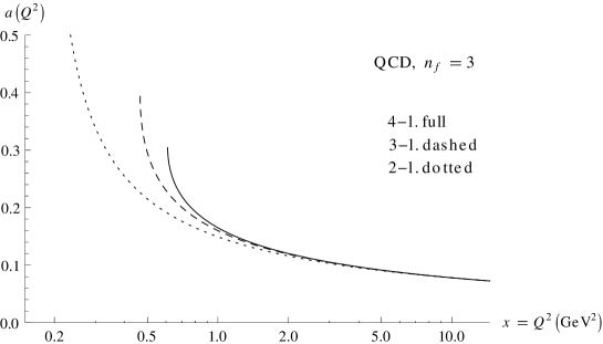
Figure 5: The effective four-loop running coupling $a^{(+)}(Q^{2})$ at positive $Q^{2}$. For comparison, the effective three-loop coupling, and the two-loop coupling, are included.

In fig. 5 we present the results for $a(Q^{2})$ at positive $Q^{2}$ – for our effective four-loop case (35), the effective three-loop case (38), and the two-loop case (37). We recall that these couplings were adjusted so that they all agree with the value of $0.07245$ at the reference scale $\mu^{2}_{\rm in}=(3m_{c})^{2}\approx 14.516\ {\rm GeV}^{2}$. The resulting $\Lambda$ scales appearing in the variables $z$ of eq. (27), are: $\Lambda\approx 0.282,0.459,0.122$ GeV, for the two-loop, the effective three-loop, and the effective four-loop case, respectively.

In fig. 6(a) the discontinuity function $\rho_{1}(\sigma)={\rm Im}a(-\sigma-i\epsilon)$ is presented. The Landau branching point $\sigma_{b}=-Q_{b}^{2}\approx-0.61\ {\rm GeV}^{2}$ is clearly visible. In fig. 6(b) the comparison of this result with those of the effective three-loop case

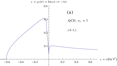
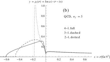
Figure 6: (a) The discontinuity function $\rho_{1}(\sigma)={\rm Im}a^{(+)}(Q^{2}=-\sigma-i\epsilon)$ as a function of $\sigma$; (b) for comparison, $\rho_{1}(\sigma)$ for the effective three-loop case, and for the two-loop case, are included.

and the two-loop case are presented. From here we can see that the branching point $Q_{b}^{2}$ increases when the (effective) loop level increases: $Q_{b}^{2}\approx 0.175,0.465,0.610\ {\rm GeV}^{2}$ ($Q_{b}\approx 0.418,0.682,0.781$ GeV) in the two-loop, the effective three-loop, and the effective four-loop case, respectively. It is interesting that the value of the coupling at the respective branching point is infinite in the two-loop case (also $\rho_{1}$ is infinite there), and finite in the effective three and four-loop cases (with the values there: $a_{b}\approx 0.398,0.307$, respectively); this can be seen in fig. 5.

If we use in our effective four-loop case minus sign in front of $\sqrt{\omega_{2}}$ of eqs. (24), i.e., the solution $a^{(-)}(Q^{2})$, eq. (36), it turns out that the numerical results are very similar to the case $a^{(+)}(Q^{2})$, as it should be, except for at small values of $|Q^{2}|$. In fig. 7(a) we compare, at positive $Q^{2}$, the running coupling $a^{(-)}$ with the previously presented coupling $a^{(+)}$. In fig. 7(b), the discontinuity functions $\rho_{1}(\sigma)$ are compared for the two cases. The $\Lambda$ scale for $a^{(-)}$ is very high: $\Lambda\approx 0.560$ GeV, compared to $\Lambda\approx 0.122$ GeV for $a^{(+)}$. Nonetheless, the Landau branching point is only a little higher: $Q_{b}\approx 0.832$ GeV ($Q_{b}\approx 0.781$ GeV for $a^{(+)}$).

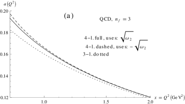
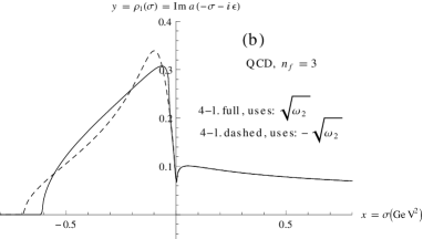
Figure 7: (a) The four-loop effective running couplings $a^{(+)}$ (full line) and $a^{(-)}$ (dashed line), at positive $Q^{2}$; (b) The discontinuity function $\rho_{1}(\sigma)={\rm Im}a(Q^{2}=-\sigma-i\epsilon)$ as a function of $\sigma$ in these two cases.

The branching point in the case of $a^{(-)}$ is the branching point of the Lambert function $W_{\mp 1}(z_{b})=-1$ ($z_{b}=-1/e$; $Q_{b}^{2}\approx 0.692\ {\rm GeV}^{2}$), as argued earlier in this Subsection, and the expression under the square root in $a^{(-)}(Q^{2})$ of eq. (36) is at this point positive. On the other hand, the expression under the square root in $a^{(+)}$, at the point where $W=-1$, is negative; therefore, as argued earlier in the previous Subsection, in this case the branching point of $a^{(+)}$ is determined by the point where the expression under the square root is zero ($Q_{b}^{2}\approx 0.610\ {\rm GeV}^{2}$).

In this context, we mention that the square root in eq. (35) for $a^{(+)}$ should be evaluated with caution, because at small $|Q^{2}|$ values the expression (“det”) under the square root is complex and crosses the negative axis in the complex plane. Specifically, at a fixed nonnegative argument of $\phi$ ($0\geq\phi\leq\pi$), when $|Q^{2}|$ decreases from from the asymptotic region ($|Q^{2}|=+\infty$) along the ray towards the origin, this expression ’det’ varies continuously in the complex plane from the 1st quadrant counterclockwise in the following order: 1st $\to$ 2nd $\to$ 3rd $\to$ 4th (when $\phi<0$, ’det’ travels in the clockwise direction, since ${\rm det}(-\phi)={\rm det}(\phi)^{\ast}$). This continuity in the variation of the argument of ’det’ (between zero and $2\pi$) must be reflected also in the square root ($\sqrt{{\rm det}}$). However, the numerical softwares usually assign the values ${\rm Arg}({\rm det})$ ($\equiv\psi$) in the interval $(-\pi,\pi)$, and such assignment would lead to spurious discontinuities of $\sqrt{|{\rm det}|}\exp(i\psi/2)$ when ’det’ crosses the negative semiaxis. This means that the square root in eq. (35) for $a^{(+)}$ must be implemented, for $Q^{2}=|Q^{2}|\exp(i\phi)$ and ${\rm det}=|{\rm det}|\exp(i\psi)$, in any numerical evaluation, in the following way:

• If $\phi\geq 0$: when $\psi\geq 0$ then $\sqrt{{\rm det}}=\sqrt{|{\rm det}|}\exp(i\psi/2)$; when $\psi<0$ then $\sqrt{{\rm det}}=\sqrt{|{\rm det}|}\exp(i(\psi+2\pi)/2)$.

• If $\phi<0$: when $\psi\leq 0$ then $\sqrt{{\rm det}}=\sqrt{|{\rm det}|}\exp(i\psi/2)$; when $\psi>0$ then $\sqrt{{\rm det}}=\sqrt{|{\rm det}|}\exp(i(\psi-2\pi)/2)$.

In the case of $a^{(-)}$ this rule for the evaluation of $\sqrt{{\rm det}}$ does not lead to any change of the result when compared to the naive evaluation of $\sqrt{{\rm det}}$, as already argued in the previous subsection.

The presented effective four-loop numerical evaluations based on our formulas (35)-(36) were cross-checked by performing the numerical RGE integration in the complex plane of $\ln(Q^{2}/\mu^{2}_{\rm in})$, applying the same initial condition $a=0.07245$ at $Q^{2}=\mu^{2}_{\rm in}$. The formulas (35)-(36) are, of course, numerically much more efficient than the numerical RGE integration in the complex plane. This practical usefulness is, in fact, the main motivation for deriving and presenting the explicit solutions eqs. (35)-(36) in the context of QCD.

V Effective five-loop case

V.1 Five-loop ansatz for $f(u)$

We take $f(u)$ in the form

$$f(u)=u+a_{0}+\frac{a_{1}}{u}+\frac{a_{2}}{u^{2}},$$ (41)

where $a_{0},$ $a_{1}$ and $a_{2}$ are arbitrary (real) numbers. We will show how to reproduce the chosen coefficients of the $\beta$-function up $\sim a^{6}$

$$\beta(a)=\beta_{0}a^{2}~{}(1+c_{1}a+c_{2}a^{2}+c_{3}a^{3}+c_{4}a^{4})+{\cal O}(a^{7})\ .$$

Thus, we consider the $\beta$-function ansatz as in the previous section

$$\beta(a)=-\frac{Aa^{2}}{2}\frac{B/f_{u}^{\prime}(u)}{1-1/f(u)},$$

where $f(u)$ is now given in eq. (41). In this effective “five-loop” case, we repeat the same procedure as was applied in the effective “four-loop” case in subsec. IV.1, except that now the expansion of $1/f^{{}^{\prime}}(u)$ must be performed up to $\sim a^{4}$. Equation (19) and the first two relations in eq. (22) are reproduced. However, the third relation in eq. (22) is modified due to the presence of $a_{2}$,

$$((a_{0}-1)^{2}+2a_{2})(B/2)^{3}=c_{3}\ ,$$

and, additionally, we get a relation involving $c_{4}$

$$a_{2}+a_{1}(a_{0}-1)-(a_{0}-1)^{3}+a_{1}^{2}=c_{4}/c_{1}^{4}\equiv\omega_{3}.$$

Thus, we obtain

$$B=2c_{1},\quad A=\beta_{0}/c_{1}\ ,$$ (42)

and the other three relations take the form

$$a_{1}-a_{0}+1=c_{2}/c_{1}^{2}\equiv\omega_{1},$$

$$(a_{0}-1)^{2}+2a_{2}=c_{3}/c_{1}^{3}\equiv\omega_{2},$$

$$a_{2}+a_{1}(a_{0}-1)-(a_{0}-1)^{3}+a_{1}^{2}=c_{4}/c_{1}^{4}\equiv\omega_{3}.$$

As a consequence, the system of the first and the second equation is

$$a_{1}=\omega_{1}+a_{0}-1,$$

$$a_{2}=(\omega_{2}-(a_{0}-1)^{2})/2.$$ (43)

After substituting this in the last equation we obtain

$$(\omega_{2}-(a_{0}-1)^{2})/2+(\omega_{1}+a_{0}-1)(a_{0}-1)$$

$$-(a_{0}-1)^{3}+(\omega_{1}+a_{0}-1)^{2}=\omega_{3},$$

which can be transformed to a form of cubic equation for $a_{0}$

$$-(a_{0}-1)^{3}+\frac{3}{2}(a_{0}-1)^{2}+3\omega_{1}(a_{0}-1)=\omega_{3}-\omega^{2}_{1}-\omega_{2}/2.$$ (44)

This is the cubic equation that has either one real or three real solutions. The knowledge of $a_{0}$ gives the values of $a_{1}$ and $a_{2}$ via eqs. (43).

V.2 Cardano solution to cubic equation

The solution to cubic equation has been found by Cardano Cardano1 ; Cardano2 . Any cubic equation can be transformed to the form without the second power of the unknown variable $x$

$$x^{3}+px+q=0.$$ (45)

The result for $x$ is given by the Cardano formula

$$x=\sqrt[3]{-\frac{q}{2}+\sqrt{\frac{q^{2}}{4}+\frac{p^{3}}{27}}}+\sqrt[3]{-\frac{q}{2}-\sqrt{\frac{q^{2}}{4}+\frac{p^{3}}{27}}}.$$ (46)

The type of solution is determined by the sign of the value of $\tau$

$$\tau\equiv\frac{q^{2}}{4}+\frac{p^{3}}{27}.$$ (47)

If $\tau$ is real and positive, there is one real root and two complex ones; if $\tau<0$, there are three distinct real roots. The case $\tau=0$ corresponds to the three real roots but two of them coincide. The expression (46) represents several (nine) possible roots. The true roots of eq. (45) are only those for which the product of the two terms in eq. (46) is equal to $-p/3$

$$\sqrt[3]{-\frac{q}{2}+\sqrt{\frac{q^{2}}{4}+\frac{p^{3}}{27}}}\sqrt[3]{-\frac{q}{2}-\sqrt{\frac{q^{2}}{4}+\frac{p^{3}}{27}}}=-\frac{p}{3}\ .$$ (48)

This appears to hold even in the most general case when $p$ and $q$ (and thus $\tau$) are nonreal complex numbers.

V.3 Equation for $a_{0}$

We write eq. (44) in the form

$$x^{3}-\frac{3}{2}x^{2}-3\omega_{1}x+(\omega_{3}-\omega^{2}_{1}-\omega_{2}/2)=0,$$ (49)

where $x=a_{0}-1,$ and transform it to the form without the quadratic terms

$$\left(x-\frac{1}{2}\right)^{3}-\left(\frac{3}{4}+3\omega_{1}\right)\left(x-\frac{1}{2}\right)-\frac{1}{4}+(\omega_{3}-\omega^{2}_{1}-\omega_{2}/2)-\frac{3}{2}\omega_{1}=0.$$ (50)

Thus, to obtain $a_{0}$ we can use the solution (46) for the variable $\left(x-\frac{1}{2}\right)\equiv(a_{0}-3/2)$, by substituting

$$p=-\frac{3}{4}-3\omega_{1},\quad q=-\frac{1}{4}+\omega_{3}-\omega^{2}_{1}-\omega_{2}/2-\frac{3}{2}\omega_{1}\ .$$ (51)

Since in this case all the coefficients are real, we should obtain at least one real root. After finding $a_{0}$, we obtain $a_{1}$ and $a_{2}$ from eqs. (43).

V.4 The inverse function for $f(u)$

Knowing explicitly the coefficients $a_{0},$ $a_{1}$ and $a_{2}$ in the ansatz (41), we have

$$-W(z)=u+a_{0}+\frac{a_{1}}{u}+\frac{a_{2}}{u^{2}},$$ (52)

where $u=2/(Ba)=1/(c_{1}a)$, and $z$ is given in eq. (27). We rewrite eq. (52) in the form

$$u^{3}+(a_{0}+W)u^{2}+a_{1}u+a_{2}=0,$$

that is again the usual cubic equation. We can rewrite it in the form

$$\left(u+(a_{0}+W)/3\right)^{3}+\left(a_{1}-(a_{0}+W)^{2}/3\right)\left(u+(a_{0}+W)/3\right)$$ (53)

$$-a_{1}(a_{0}+W)/3+2(a_{0}+W)^{3}/27+a_{2}=0\ ,$$

i.e., we eliminate the term with the second power. Thus, to solve for the running coupling $a(Q^{2})\equiv 1/(c_{1}u)$, we can use the Cardano solution (46) where

$$x=x(z) = u+\frac{1}{3}\left(a_{0}+W(z)\right)=\frac{1}{c_{1}a(Q^{2})}+\frac{1}{3}\left(a_{0}+W(z)\right)\ \Rightarrow$$

$$a(Q^{2}) = \frac{1}{c_{1}}\frac{1}{\left[x(z)-\left(a_{0}+W(z)\right)/3\right]}\ ,$$ (54)

$$p(z) = -\frac{1}{3}\left(a_{0}+W(z)\right)^{2}+\omega_{1}+a_{0}-1\ ,$$ (55)

$$q(z) = \frac{2}{27}\left(a_{0}+W(z)\right)^{3}-\frac{\omega_{1}+a_{0}-1}{3}\left(a_{0}+W(z)\right)+\frac{\omega_{2}-(a_{0}-1)^{2}}{2}\ .$$ (56)

As in sec. IV, $W(z)=W_{\mp 1}(z)$ is again the Lambert function, with $z$ defined in eq. (27), and $W=W_{-1}(z)$ when $0\leq\phi<\pi$, and $W=W_{+1}(z)$ when $-\pi\leq\phi<0$ (where: $Q^{2}=|Q^{2}|e^{i\phi}$). Now, for a general complex $z$ (or: $Q^{2}$), the coefficients $p(z)$ and $q(z)$ are complex numbers, too, as are the roots $x(z)$ and thus $a(Q^{2})$. The restriction (48) is valid also in this general complex case.

V.5 Cut structure and analyticity

An advantage of the effective five-loop solution, eqs. (54)-(56) and (46), in comparison with the four-loop solution, eqs. (35) and (36), is that the cubic equation (44) for the coefficient $a_{0}$ always has at least one real root. This means that we do not obtain any restriction on the sign of the RSch coefficients $c_{j}$ ($j=2,3,4$) imposed by the reality of the running coupling $a(Q^{2})$ at large positive $Q^{2}$, in contrast to the effective four-loop case (where $c_{3}<0$ leads to a nonreal $a_{0}$ and nonreal $a(Q^{2})$ at large positive $Q^{2}$).

As has been shown in the previous section, dedicated to the effective four-loop case, the cut structure of $a(Q^{2})$ in the plane of complex $z$ (or: of complex $Q^{2}$) has two origins. The first origin of the cuts is the multivalued nature of the Lambert W function. In the effective five-loop case, the corresponding cuts in $z$-plane repeat completely their analogs in the effective four-loop case; the corresponding Riemann surface remains unchanged, and also the phase relation caused by the power-like relation between the complex variable $z$ and the complex variable $Q^{2}$, eq. (27), remains the same.

The second origin for the cuts in the complex $z$-plane is that the running coupling $a(Q^{2})$ is a composite function of the Lambert function, that composite function having multivalued nature, too. In the effective five-loop case of this section, the cut structure in the $z$-plane is different from the corresponding cut structure in the effective four-loop case (33) since the map from the $W$-partitions to the running coupling has a more complicated structure, eqs. (54)-(56) and (46). To identify the start of the cut in the complex $W$-plane, we have to analyze the roots of the quantity $\tau$, eq. (47), i.e., roots of the sixth power polynomial described in terms of the variable $a_{0}+W(z)$, cf. eqs. (55)-(56). At present, it is impossible to find analytic expressions for the roots of polynomials of power higher than four. However there are many numerical tools to perform that analysis (see the next subsection). In addition, the possible cuts due to the cubic roots in (46) should be taken into account. These cubic roots can produce new cuts in the partitions of the complex plane of the composite variable $\sqrt{\tau}$, which would be transformed into new cuts in the $W$-plane, and finally into new cuts in the $z$-plane (and $Q^{2}$-plane). Such a recursive mapping of the cuts is the simplest way to analyze the cut structure of the running coupling in the complex $z$-plane (and $Q^{2}$-plane), especially for the evaluation of the starting (branching) points of the cuts.

From the point of view of the analytic evaluation, a simpler representation for the solutions exists in terms of trigonometric functions Smirnov . It is not a universal representation as the representation of eq. (46). For example, for real negative $\tau$ and $p$, the trigonometric representation of eq. (46) is

$$x=2\sqrt[3]{r}\cos\left({\frac{\phi+2k\pi}{3}}\right),~{}~{}~{}~{}k=0,1,2,$$

$$r=\sqrt{-\frac{p^{3}}{27}},~{}~{}~{}~{}\cos\phi=-\frac{q}{2r}.$$

It is a more helpful form of solution for the analysis of the roots; but it is less helpful for the analysis of cuts in the complex $z$-plane, since the form of the representations is not power-like. Thus, we prefer the original form (46) of the Cardano solution for the numerical evaluation of the cuts in the complex $z$-plane.

V.6 Numerical evaluation of analytic formulas

Similarly as we did in subsec. IV.4 in the effective four-loop case, we evaluate now the analytic formulas for the running coupling $a(Q^{2})$ in the effective five-loop case, in QCD with $n_{f}=3$ and in ${\overline{\rm MS}}$ scheme. In contrast to the coefficients $c_{2}$ and $c_{3}$, the exact five-loop coefficient $c_{4}$ in ${\overline{\rm MS}}$ has not been obtained yet in the literature. However, Padé-related estimates, ref. Ellis:1997sb give the value $c_{4}\approx 123.701$ at $n_{f}=3$. We use this value in our formulas. Equation (50) for the coefficient $a_{0}$ has only one real solution, $a_{0}=-1.19666$. The running coupling $a(Q^{2})$ is obtained by using the formula (46) in conjunction with the formulas (53) and (54)-(56), and the relation (27). The same initial condition as in subsec. IV.4 is applied, i.e., eq. (40). In the effective five-loop case, this condition gives $\Lambda\approx 0.621{\rm GeV}^{2}$.

At large values of $|Q^{2}|/\Lambda^{2}\equiv u$ ($=|z|$), i.e., in the asymptotic freedom regime, this gives us the correct real solution for $a(Q^{2})$ unambiguously. However, when we move in the $Q^{2}$-complex plane along a fixed ray $\phi={\rm const}$ (where $Q^{2}=|Q^{2}|e^{i\phi}=u\Lambda^{2}ue^{i\phi}$) toward the origin, the expression under the square root in eq. (46)

$${\rm Det}_{2}(u,\phi)\left(=\tau(p,q)\right)\equiv\frac{1}{4}\left(q(u,\phi)\right)^{2}+\frac{1}{27}\left(p(u,\phi)\right)^{3}$$ (57)

changes the argument $\psi_{2}$ of ${\rm Det}_{2}=|{\rm Det}_{2}|\exp(i\psi_{2})$ continuously, and this behavior depends crucially on whether the (nonnegative fixed) $\phi$ is below or above a threshold angle $\phi_{\rm thr}$. Here, the threshold angle is determined by the condition

$${\rm Det}_{2}(u_{\rm thr},\phi_{\rm thr})=0\ \Rightarrow\phi_{\rm thr}\approx 0.0507,\ u_{\rm thr}\approx 0.314\ .$$ (58)

Figure 8: The variation of ${\rm Det}_{2}(u,\phi)$ in the complex plane, at fixed nonnegative $\phi$ ($\equiv arg(Q^{2})$), when $u$ ($\equiv|Q^{2}|/\Lambda^{2}$) is decreasing toward zero: (a) when $\phi_{\rm thr}<\phi$, the path encircles the origin; (b) when $\phi<\phi_{\rm thr}$, the path avoids encircling the origin.

It turns out that, at fixed nonnegative $\phi$ and when $u\equiv|Q^{2}|/\Lambda^{2}$ decreases toward zero, the argument $\psi_{2}$ of ${\rm Det}_{2}$ varies within the interval $(0,3\pi)$ if $\phi_{\rm thr}<\phi$, and in the interval $(-\pi/2,+\pi)$ if ($0\leq$) $\phi<\phi_{\rm thr}$ – see figs. 8(a) and (b). The square root of ${\rm Det}_{2}$ must be calculated in the way that reflects the continuous change of $\psi_{2}$ during the movement along the ray, i.e., $\sqrt{{\rm Det}_{2}}=\sqrt{|{\rm Det}_{2}|}\exp(i\psi_{2}/2)$.

The same care must be taken when evaluating the third roots in the solution (46), i.e., the third roots of

$${\rm Det}_{3\pm}(u,\phi)\equiv-\frac{1}{2}q(u,\phi)\pm\sqrt{{\rm Det}_{2}(u,\phi)}\ .$$ (59)

Again, the behavior along the $Q^{2}$-rays changes drastically when $\phi$ passes the threshold angle $\phi_{\rm thr}$.

Figure 9: The same as in fig. 8, but now for the expression ${\rm Det}_{3-}(u,\phi)$ given in eq. (59).

Figure 10: The same as in fig. 8, but now for the expression ${\rm Det}_{3+}(u,\phi)$ given in eq. (59).

The argument $\psi_{3-}$ of ${\rm Det}_{3-}$ varies in the interval $(0,+3\pi)$ if $\phi_{\rm thr}<\phi$, and in $(0,+5\pi)$ if ($0\leq$) $\phi<\phi_{\rm thr}$ – cf. figs. 9(a) and (b). The argument $\psi_{3+}$ of ${\rm Det}_{3+}$ varies in the interval $(0,+3\pi)$ if $\phi_{\rm thr}<\phi$, and in $(-\pi/2,+\pi)$ if ($0\leq$) $\phi<\phi_{\rm thr}$ – cf. figs. 10(a) and (b). The third roots in the solution (46), whose sum gives us the running complex $a(Q^{2})$, must reflect the continuous change of $\psi_{3\pm}$ during the movement along the rays, i.e., in the evaluation we must implement: $({\rm Det}_{3\pm})^{1/3}=|{\rm Det}_{3\pm}|^{1/3}\exp(i\psi_{3\pm}/3)$.

For the negative $\phi$ ($-\pi\leq\phi<0$), the evaluation of $a(Q^{2})$ is then implemented easily, using the relation $a(Q^{2\ast})=a(Q^{2})^{\ast}$.

In this way, the correct roots are chosen from the plethora of possible roots given by the expression (46), for all complex $Q^{2}$ down to $Q^{2}\to 0$. In the Appendix we specify, for the case of QCD in the ${\overline{\rm MS}}$ scheme with $n_{f}=3$ as an example, how to implement in practice (in software) the calculation of the angles $\psi_{2}$ and $\psi_{3\pm}$, and thus the evaluation of $({\rm Det_{2}})^{1/2}$ and $({\rm Det}_{3\pm})^{1/3}$. We checked that the solutions obtained in this way satisfy eq. (45) with $p$ and $q$ given in eqs. (55)-(56), and the constraint (48).

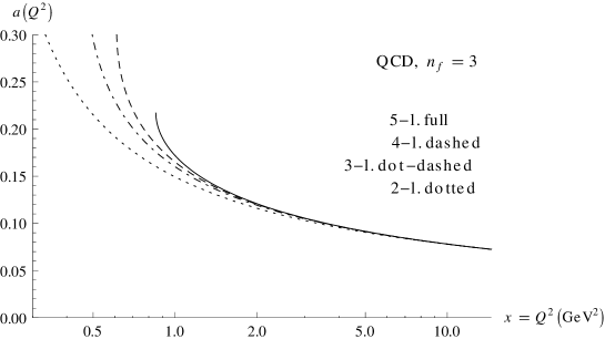
Figure 11: The effective five-loop running coupling $a^{(+)}(Q^{2})$ at positive $Q^{2}$. For comparison, the effective four- and three-loop coupling, and the two-loop coupling, are included.

In fig. 11 we present the effective five-loop running coupling, evaluated in the aforementioned way, at positive $Q^{2}$. The lower-loop couplings are included, for comparison. The figure is analogous to fig. 5, but now includes the effective five-loop case. We recall that all the couplings are adjusted to the same initial value at $Q^{2}=\mu_{\rm in}^{2}\approx 14.516\ {\rm GeV}^{2}$, eq. (40).

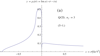
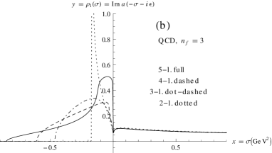
Figure 12: (a) The effective five-loop discontinuity function $\rho_{1}(\sigma)={\rm Im}a^{(+)}(Q^{2}=-\sigma-i\epsilon)$ as a function of $\sigma$; (b) for comparison, $\rho_{1}(\sigma)$ for the effective four- and three-loop case, and for the two-loop case, are included.

In fig. 12(a) we present the effective five-loop discontinuity function $\rho_{1}(\sigma)={\rm Im}a(-\sigma-i\epsilon)$. The branching point where the (Landau) cut starts is at $Q_{b}^{2}\approx 0.849\ {\rm GeV}^{2}$ ($\sigma_{b}=-Q_{b}^{2}$), i.e., at $z=-1/e$ where the Lambert function $W_{-1}(z)$ has the value $-1$ and has a branching point. In fig. 12(b), this discontinuity function is compared with those of the effective four- and three-loop case and the two-loop case. The aforementioned branching point can be inferred also from fig. 11, where we see that the (effective five-loop) coupling achieves a finite value $a_{b}\approx 0.218$ at the branching point.

In the presented ${\overline{\rm MS}}$ effective five-loop case (with $n_{f}=3$), there is another branching point, namely the one given in eq. (58), as already mentioned in the previous subsection. It corresponds to the value $|Q^{2}_{\rm thr}|\approx 0.122\ {\rm GeV}^{2}$ and $\phi=\pm\phi_{\rm thr}\approx\pm 0.0507$. This branching point is quite close to the origin, but is off the real axis. In order to see this starting point of nonanalyticity more easily, we present in fig. 13(a) the

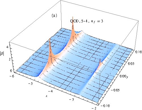
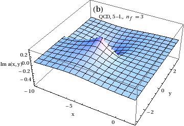
Figure 13: (a) The absolute value of the beta function $\beta(a(Q^{2}))$, for complex $Q^{2}$ ($=\mu_{\rm in}^{2}\exp(x)\exp(iy)$) near the origin; the three starting (branching) points of Landau cuts are visible as three peaks; (b) imaginary part of $a(Q^{2})$ in the entire $Q^{2}$ complex plane.

function $|\beta(a(Q^{2}))|$ at complex $Q^{2}$ not far from the origin, with axes $x=\ln(Q^{2}/\mu_{\rm in}^{2})$ (note: $\mu_{\rm in}^{2}\approx 14.516\ {\rm GeV}^{2}$) and $y=\phi$. In the figure we clearly see two peaks at $x\approx-4.79$ ($|Q^{2}|\approx 0.122\ {\rm GeV}^{2}$) and $\phi\approx\pm\phi_{\rm thr}$. Yet another peak is visible at $x\approx-2.84$ and $\phi=0$, representing the aforementioned $Q_{b}^{2}\approx 0.849\ {\rm GeV}^{2}$ branching point that is simultaneously a branching point of $W_{-1}(z)$.

In fig. 13(b) we present the imaginary part of $a(Q^{2})$ in the (almost) entire complex plane. At $y=0$ the usual discontinuity function $\rho_{1}$ is contained in this figure.

VI Conclusion

In this paper we started with the derivation of an analytic formula for the solution of the renormalization group equation (RGE) for the coupling parameter in the supersymmetric model of Novikov et al. (NSVZ, Novikov:1983uc ). We extended this analysis, by deriving analytic formulas for solutions to a class of RGE’s for the QCD coupling parameter $a(Q^{2})\equiv\alpha_{s}(Q^{2})/\pi$. The class of beta functions $\beta(a)$ in these RGE’s is of the form

$$\frac{da(Q^{2})}{d\ln Q^{2}}=-\beta_{0}a^{2}\frac{\left(1/f_{u}^{{}^{\prime}}(u)\right)}{\left(1-1/f(u)\right)}{\bigg{|}}_{u=1/(c_{1}a)}\ ,$$ (60)

where $\beta_{0}$ and $c_{1}=\beta_{1}/\beta_{0}$ are the (universal) first two coefficients in the power expansion of $\beta$ function eq. (2), and $f(u)$ is a function of the following form:

$$f(u)=u+a_{0}+\sum_{j=1}^{n}\frac{a_{j}}{u^{j}}\ .$$ (61)

We found that the solution $a(Q^{2})$, for general complex $Q^{2}$, can be written in the following simple (but implicit) form:

$$f(u)|_{u=1/(c_{1}a(Q^{2}))}=-W_{\mp 1}\left(-(\Lambda^{2}/Q^{2})^{\beta_{0}/c_{1}}\right)\ ,$$ (62)

where $W_{\mp 1}$ are two partitions (branches) of the Lambert function ($W_{-1}$ when ${\rm Im}Q^{2}\geq 0$, $W_{+1}$ when ${\rm Im}(Q^{2})<0$), and the scale $\Lambda$ is fixed by an initial condition [e.g., the condition (40)].

We showed that the $(n+1)$ real parameters $a_{j}$ ($j=0,\ldots,n$) in function $f(u)$ can be adjusted so that the power expansion of $\beta(a)$ reproduces the $(n+3)$-loop polynomial beta function in any chosen renormalization scheme (RSch), i.e., for any chosen values of the RSch parameters $c_{2},\ldots,c_{n+2}$ in the expansion (2). In order to obtain an analytic (i.e., explicit) formula for $a(Q^{2})$, the polynomial-type of relation (62) has to be solved. This we did explicitly in the (effective) four-loop case ($n=1$) and in the effective five-loop case ($n=2$). The (effective) three-loop case ($n=0$), i.e., the case of the beta function of eq. (3), was solved in ref. Gardi:1998qr (their sec. 4).

We discussed in detail the (non)analyticity structure of the RGE solution in the complex $Q^{2}$ plane. We presented numerical evaluation of the obtained formulas in the case of the effective four-loop and the effective five-loop $\beta$ (i.e., for $n=1,2$) in the ${\overline{\rm MS}}$ RSch and with the number of active quark flavors $n_{f}=3$.

It is, in principle, possible to go even further, to $n=3$ (effective six-loop case). In such a case eq. (62) becomes a quartic equation in $u$ ($\equiv 1/(c_{1}a)$), i.e., the highest order polynomial equation for which an analytic (explicit) formula exists: Ferrari formula. In any case, the (effective) five-loop formula found in sec. V is already a good approximation at sufficiently high $|Q^{2}|$ (e.g., at $|Q^{2}|>2\ {\rm GeV}^{2}$, cf. fig. 11). Any numerical evaluation of perturbative results at five-loop order can be performed by using the (effective) five-loop formula for $a(Q^{2})$ found in this paper.

Appendix A Implementation of arguments in the effective five-loop case

In the effective five-loop case of sec. V, for the specific case of QCD with $n_{f}=3$ in ${\overline{\rm MS}}$ scheme, the results of the numerical evaluation of the analytic formula for the running coupling $a(Q^{2})$ (with $Q^{2}$ in general complex) were presented in subsec. V.6. For such evaluations, we need to know in practice how to implement (in software) the calculation of the angles $\psi_{2}$ and $\psi_{3\pm}$, leading to the evaluation of $({\rm Det}_{2})^{1/2}$ and $({\rm Det}_{3\pm})^{1/3}$, where ${\rm Det}_{2}$ and ${\rm Det}_{3\pm}$ are defined in eqs. (57) and (59). The running of these quantities in their own complex planes, when $u$ ($\equiv|Q^{2}|/\Lambda^{2}$) decreases from infinity towards zero, at fixed $\phi$ (we recall: $Q^{2}=|Q^{2}|e^{i\phi}$, $-\pi<\phi\leq\pi$) is presented in figs. 8, 9, 10, respectively (in subsec. V.6). We note that the softwares, such as Mathematica Math8 , assign to the complex numbers the arguments (angles) in the interval $]-\pi,\pi]$, i.e., they are not capable of keeping track of the correct arguments once those arguments go outside this interval. Therefore, in order to implement in practice the unambiguous calculation of $\psi_{2}$ and $\psi_{3\pm}$, we need to lift the ambiguity $\psi_{j}\leftrightarrow\psi_{j}+2\pi k$ ($j=2,3-,3+$; $k$ is integer)) obtained by the numerical evaluations of these arguments. Below we show how this ambiguity is lifted in practice in the case of subsec. V.6, i.e., the effective five-loop QCD case in ${\overline{\rm MS}}$ scheme and with $n_{f}=3$.

1. For ${\rm Det}_{2}(u,\phi)\equiv|{\rm Det}_{2}(u,\phi)|\exp(i\psi_{2})$:

   • If $\phi_{\rm thr}\leq\phi\leq\pi$ (fig. 8(a)), we can check that ${\rm Im}{\rm Det}_{2}(u_{\rm thr},\phi)<0$. Therefore: (a) when ${\rm Im}{\rm Det}_{2}\geq 0$ and $u>u_{\rm thr}$, we have $0\leq\psi_{2}\leq\pi$; (b) when ${\rm Im}{\rm Det}_{2}\geq 0$ and $u<u_{\rm thr}$, we have $2\pi\leq\psi_{2}\leq 3\pi$; (c) when ${\rm Im}{\rm Det}_{2}<0$, we have $\pi<\psi_{2}<2\pi$.

   • If ($0\leq$) $\phi<\phi_{\rm thr}$ (fig. 8(b)), we have $-\pi/2<\psi_{2}<\pi$.

2. For ${\rm Det}_{3-}(u,\phi)\equiv|{\rm Det}_{3-}(u,\phi)|\exp(i\psi_{3-})$:

   • If $\phi_{\rm thr}\leq\phi\leq\pi$ (fig. 9(a)), we can check that for $u_{0}\equiv u_{\rm thr}+0.001$ we have ${\rm Im}{\rm Det}_{3-}(u_{0},\phi)<0$ and that it represents a point in the left sector of the two sectors with ${\rm Im}{\rm Det}_{3-}<0$ (see fig. 9(a); further, for $\phi$ sufficiently large, there is only one sector with ${\rm Im}{\rm Det}_{3-}<0$). Therefore: (a) when ${\rm Im}{\rm Det}_{3-}\geq 0$ and $u>u_{0}$, we have $0\leq\psi_{3-}\leq\pi$; (b) when ${\rm Im}{\rm Det}_{3-}\geq 0$ and $u<u_{0}$, we have $2\pi\leq\psi_{3-}\leq 3\pi$; (c) when ${\rm Im}{\rm Det}_{3-}<0$, we have $\pi<\psi_{3-}<2\pi$.

   • If ($0\leq$) $\phi<\phi_{\rm thr}$ (fig. 9(b)), we can check that the transition of ${\rm Det}_{3-}$ from the 4th to the 5th quadrant takes place at u between $u_{4}\equiv u_{\rm thr}+0.0014$ and $u_{5}\equiv u_{\rm thr}-0.0017$ ($u_{5}<u_{4\to 5}<u_{4}$); and that for $u=u_{7}\equiv 0.174$ the quantity ${\rm Det}_{3-}$ is in the 7th quadrant. Therefore: (a) when ${\rm Im}{\rm Det}_{3-}\geq 0$ and $u>u_{4}$, we have $0\leq\psi_{3-}\leq\pi$; (b) when ${\rm Im}{\rm Det}_{3-}\geq 0$ and $u_{7}<u<u_{4}$, we have $2\pi\leq\psi_{3-}\leq 3\pi$; (b) when ${\rm Im}{\rm Det}_{3-}\geq 0$ and $u<u_{7}$, we have $4\pi\leq\psi_{3-}\leq 5\pi$; (d) when ${\rm Im}{\rm Det}_{3-}<0$ and $u>u_{5}$, we have $\pi<\psi_{3-}<2\pi$; (e) when ${\rm Im}{\rm Det}_{3-}<0$ and $u<u_{5}$, we have $3\pi<\psi_{3-}<4\pi$;

3. For ${\rm Det}_{3+}(u,\phi)\equiv|{\rm Det}_{3+}(u,\phi)|\exp(i\psi_{3+})$:

   • If $\phi_{\rm thr}\leq\phi\leq\pi$ (fig. 10(a)), we can check that at $u_{\rm low}=0.174$ we have ${\rm Im}{\rm Det}_{3+}<0$. Therefore, (a) when ${\rm Im}{\rm Det}_{3+}\geq 0$ and $u>u_{\rm low}$, we have $0\leq\psi_{3+}\leq\pi$; (b) when ${\rm Im}{\rm Det}_{3+}\geq 0$ and $u<u_{\rm low}$, we have $2\pi\leq\psi_{3+}\leq 3\pi$; (c) when ${\rm Im}{\rm Det}_{3+}<0$, we have $\pi<\psi_{3+}<2\pi$.

   • If ($0\leq$) $\phi<\phi_{\rm thr}$ (fig. 10(b)), we have $-\pi/2<\psi_{3+}<\pi$.

When the number of effective quark flavors $n_{f}$ changes, or the renormalization scheme changes away from ${\overline{\rm MS}}$, the above rules in general do not get modified qualitatively, but quantitatively the values $\phi_{\rm thr}$, $u_{\rm thr}$, $u_{4}$, $u_{5}$, etc. do change.

References

- (1) E. Gardi, G. Grunberg and M. Karliner, “Can the QCD running coupling have a causal analyticity structure?,” JHEP 9807 (1998) 007 [arXiv:hep-ph/9806462].
- (2) B. A. Magradze, “The gluon propagator in analytic perturbation theory,” arXiv:hep-ph/9808247; “A novel series solution to the renormalization group equation in QCD,” Few Body Syst. 40 (2006) 71 [arXiv:hep-ph/0512374].
- (3) V. A. Novikov, M. A. Shifman, A. I. Vainshtein and V. I. Zakharov, “Exact Gell-Mann-Low function of supersymmetric Yang-Mills theories from instanton calculus,” Nucl. Phys. B 229 (1983) 381; D. R. T. Jones, “More on the axial anomaly in supersymmetric Yang-Mills theory,” Phys. Lett. B 123 (1983) 45.
- (4) N.N. Bogoliubov and D.V. Shirkov, Introduction to the Theory of Quantum Fields, New York, Wiley, 1959; 1980.
- (5) R. Oehme, “Analytic structure of amplitudes in gauge theories with confinement,” Int. J. Mod. Phys. A 10, 1995 (1995) [arXiv:hep-th/9412040].
- (6) D. V. Shirkov and I. L. Solovtsov, “Analytic model for the QCD running coupling with universal value,” Phys. Rev. Lett. 79 (1997) 1209 [arXiv:hep-ph/9704333].
- (7) G. M. Prosperi, M. Raciti and C. Simolo, “On the running coupling constant in QCD,” Prog. Part. Nucl. Phys. 58, 387 (2007) [arXiv:hep-ph/0607209]; D. V. Shirkov and I. L. Solovtsov, “Ten years of the analytic perturbation theory in QCD,” Theor. Math. Phys. 150, 132 (2007) [arXiv:hep-ph/0611229]; G. Cvetič and C. Valenzuela, “Analytic QCD - a short review,” Braz. J. Phys. 38, 371 (2008) [arXiv:0804.0872 [hep-ph]]; A. P. Bakulev, “Global Fractional Analytic Perturbation Theory in QCD with selected applications,” Phys. Part. Nucl. 40, 715 (2009) (in Russian) [arXiv:0805.0829 [hep-ph]];
- (8) G. Cvetič and R. Kögerler, “Applying generalized Padé approximants in analytic QCD models,” Phys. Rev. D 84, 056005 (2011) [arXiv:1107.2902 [hep-ph]].
- (9) D. R. T. Jones, private communication.
- (10) R. M. Corless, G. H. Gonnet, D. E. G. Hare, D. J. Jeffrey, D. E. Knuth, “On the Lambert W function,” Adv. Comput. Math. 5, 329-359 (1996).
- (11) Mathematica 8.0.1, Wolfram Co.
- (12) G. Cardano, Practica arithmetice et mensurandi singularis, Milan, (1539).
- (13) G. Cardano, Artis magnae, sive de regulis algebraicis, Nuremberg, (1545).
- (14) C. Amsler et al. [Particle Data Group], “Review of particle physics,” Phys. Lett. B 667, 1 (2008).
- (15) K. Nakamura et al. [Particle Data Group], “Review of particle physics,” J. Phys. G 37, 075021 (2010).
- (16) K. G. Chetyrkin, B. A. Kniehl and M. Steinhauser, “Strong coupling constant with flavour thresholds at four loops in the scheme,” Phys. Rev. Lett. 79, 2184 (1997) [arXiv:hep-ph/9706430].
- (17) V.I. Smirnov, Lehrgang der höheren Mathematik, Teil I, (Course in higher mathematics. Part I). Übers. aus dem Russischen (German). Hochschulbücher für Mathematik, Bd. 1. Berlin: VEB Deutscher Verlag der Wissenschaften. 449 S. (1986).
- (18) J. R. Ellis, I. Jack, D. R. T. Jones, M. Karliner, M. A. Samuel, “Asymptotic Padé approximant predictions: up to five loops in QCD and SQCD,” Phys. Rev. D57, 2665-2675 (1998). [hep-ph/9710302].