Continuum extrapolation of $B_{K}$ with staggered fermions

Abstract:

We report on recent progress in the calculation of $B_{K}$ using HYP-smeared staggered fermions on the MILC asqtad lattices. Our main focus is on the continuum extrapolation, which is done using (up to) four different lattice spacings—$a\approx$ 0.12, 0.09, 0.06 and 0.045 fm. Since Lattice 2010, we have reduced the statistical errors on the $a\approx 0.09\;$fm lattices by a factor of $\sim 3$, and roughly doubled the size of the $a\approx 0.045\;$fm ensemble. We find that these improvements have a very significant impact on the continuum extrapolation, with the $a\approx 0.12\;$fm data lying outside the range of applicability of simple functional forms. Hence we use only the three smallest lattice spacings to perform the extrapolation, finding $\hat{B}_{K}=B_{K}(\text{RGI})=0.725\pm 0.004(\text{stat})\pm 0.038(\text{sys})$. This value is consistent with our published value from 2010 (based the three coarsest lattice spacings), but has smaller errors.

1 Introduction

The calculation of the kaon mixing matrix element $B_{K}$ is one of the successes of lattice QCD. Results with all errors controlled are available with different fermion discretizations, the most recent entry being that using Wilson fermions [1]. For a summary, see Refs. [2] and [3]. There is some tension between these results, which needs to be resolved in order to know whether the Standard Model can describe CP-violation in kaon mixing.

In this proceedings we update our results for $B_{K}$. These are obtained using improved staggered fermions, specifically HYP-smeared valence quarks on asqtad sea-quarks. We describe here results obtained with chiral fitting functions from SU(2) staggered chiral perturbation theory (SChPT), which give our most reliable results [4]. We compare our results to those obtained a year ago and presented at Lattice 2010 [5]. In companion proceedings we update the analysis based on SU(3) SChPT [6] and discuss strategies for dealing with correlations in chiral fits [7].

Table 1 lists all the ensembles on which we have calculated $B_{K}$, and notes which results have changed in the last year. In particular, since Lattice 2010 we have accumulated higher statistics on the C2, C5, F1, U1 ensembles and added a new measurement on S2. Of these, the most important updates are those on F1 and U1, since they are used (together with C3 and S1) to do our continuum extrapolation. We focus on this issue here. The other updates, as well as the yet unanalyzed ensemble S2, provide information on the sea-quark mass dependence at multiple lattice spacings.

$a$ (fm)	$am_{l}/am_{s}$	geometry	ID	ens $\times$ meas	$B_{K}$($\mu=2$ GeV)	status
0.12	0.03/0.05	$20^{3}\times 64$	C1	$564\times 1$	0.556(14)	old
0.12	0.02/0.05	$20^{3}\times 64$	C2	$486\times 9$	0.568(16)	update
0.12	0.01/0.05	$20^{3}\times 64$	C3	$671\times 9$	0.566(5)	old
0.12	0.01/0.05	$28^{3}\times 64$	C3-2	$275\times 8$	0.570(4)	old
0.12	0.007/0.05	$20^{3}\times 64$	C4	$651\times 10$	0.563(5)	old
0.12	0.005/0.05	$24^{3}\times 64$	C5	$509\times 9$	0.566(4)	update
0.09	0.0062/0.031	$28^{3}\times 96$	F1	$995\times 9$	0.527(4)	update
0.09	0.0031/0.031	$40^{3}\times 96$	F2	$850\times 1$	0.551(9)	update
0.06	0.0036/0.018	$48^{3}\times 144$	S1	$744\times 2$	0.537(7)	old
0.06	0.0025/0.018	$56^{3}\times 144$	S2	$198\times 9$	-NA-	new
0.045	0.0028/0.014	$64^{3}\times 192$	U1	$705\times 1$	0.530(7)	update

Table 1: MILC asqtad ensembles used to calculate $B_{K}$. $am_{\ell}$ and $am_{s}$ are the masses, in lattice units, of the light and strange sea quarks, respectively. “ens” indicates the number of configurations on which “meas” measurements are made. The results for $B_{K}(\text{NDR},2\text{ GeV})$ are obtained using the SU(2) SChPT fits (4X3Y-NNLO) discussed in the text.

2 Chiral fits

In our numerical study, our lattice kaons are composed of valence (anti)quarks with masses $m_{x}$ and $m_{y}$. On each MILC ensemble, we use 10 valence masses:

$$am_{x},am_{y}=am_{s}\times{n}/{10}\qquad\text{with}\qquad n=1,2,3,\ldots,10,$$ (1)

where $am_{s}$ is the strange sea quark mass. In our standard fits we extrapolate to $am_{d}^{\rm phys}$ using the lowest 4 values for $am_{x}$ (the “X-fit”—done at fixed $am_{y}$), and then extrapolate to $m^{\textrm{phys}}_{s}$ using the highest 3 values of $am_{y}$ (“Y-fit”). As described in Ref. [4], these choices keep us in the regime where we expect next-to-leading order (NLO) SU(2) ChPT to be reasonably accurate. The X-fits described here are done to the form predicted by NLO partially quenched SChPT (and given in Ref. [4]), augmented by a single analytic term of next-to-next-to-leading order (NNLO). The $am_{y}$ dependence (which is not controlled by ChPT) is very close to linear and we use a linear fit for our central values. We dub this entire fitting procedure the “4X3Y-NNLO fit”, and use it for our central values. Other choices (e.g. NLO vs. NNLO) are used to estimate fitting systematics.

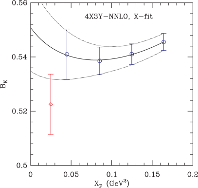
(a) Lattice 2010

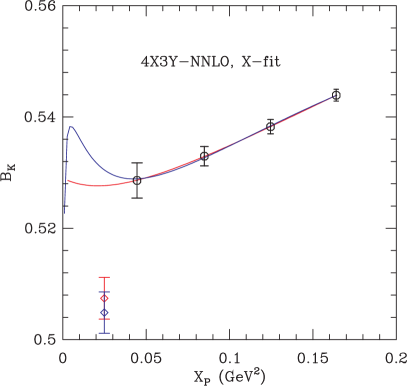
(b) Lattice 2011

Figure 1: X-fits to $B_{K}(1/a)$ for the F1 ensemble, with 1 measurement/configuration (left) and with 9 measurements/configuration (right). $X_{P}$ is the mass-squared of the $\bar{x}x$ valence pion, and we fix $am_{y}=0.031$ (the heaviest value). In the right panel, the blue curve includes finite-volume (FV) corrections, while the red curve does not. FV corrections are not included in the left panel. Extrapolated results (diamonds) have known taste-breaking discretization errors removed and thus do not lie on the curves.

Examples of the X-fits are shown in Fig. 1. Here we compare results on the F1 ensemble from Lattice 2010 with those from our present dataset. In each panel, a fit to the SChPT form is shown, together with the result after extrapolating $am_{x}\to am_{d}^{\rm phys}$ and removing known discretization errors. For details of this procedure, see Ref. [4].

The addition of 8 extra measurements per configuration reduces the statistical errors by $\sim 3$, as expected. In addition, the central values shift down by about $1\sigma$, leading to a correspondingly lower value of $B_{K}$. We have also now incorporated finite volume corrections, as predicted by NLO SChPT, into the fitting function [8].

3 Continuum Extrapolation

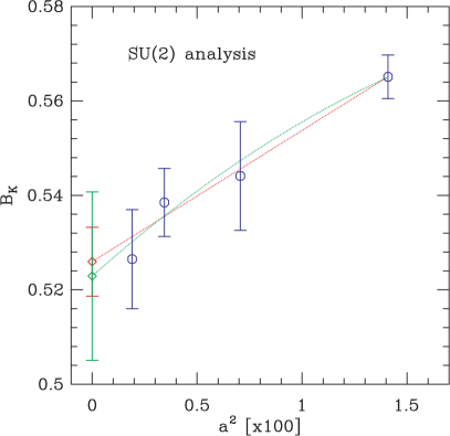
(a) Lattice 2010

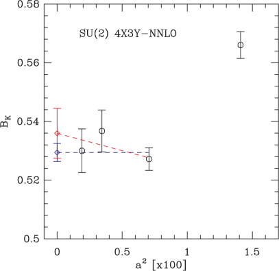
(b) Lattice 2011

Figure 2: Continuum extrapolation of $B_{K}(\mu=2\;{\rm GeV})$ versus $a^{2}$ (in units of $0.01\;{\rm fm}^{2}$). The left panel shows results from Lattice 2010, with linear and quadratic fits. The right panel shows our updated results, with constant and linear fits to the leftmost three points.

We do our continuum extrapolation using the four lattices with $am_{\ell}/am_{s}=0.2$. Figure 2 shows how this extrapolation is changed by our updated results. Clearly, the most significant change is for the F1 ensemble, where the downward shift rules out the possibility of a straightforward extrapolation using all four points. We thus first consider extrapolations based only on the smallest three values of $a$. The figure shows results both for a constant and a linear fit, which have good $\chi^{2}/d.o.f$ as listed in Table 2.

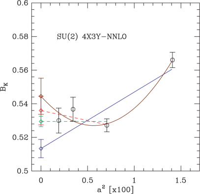
(a) Unconstrained

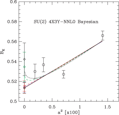
(b) Bayesian

Figure 3: Continuum extrapolations of $B_{K}(\mu=2\;{\rm GeV})$ with different fitting choices. Fits are described in the text.

fit type	# data	fit function	$\chi^{2}$/d.o.f	$\chi^{2}$/d.o.f. (Bayes)
const	3	$c_{1}$	0.70	-NA-
lin3	3	$c_{1}+c_{2}a^{2}$	0.73	-NA-
lin4	4	$c_{1}+c_{2}a^{2}$	6.35	-NA-
quad	4	$c_{1}+c_{2}a^{2}+c_{3}a^{4}$	1.44	4.39
a2a2g2	4	$c_{1}+c_{2}a^{2}+c_{3}a^{2}\alpha_{s}(a)$	1.66	4.16
a2g4	4	$c_{1}+c_{2}a^{2}+c_{3}\alpha_{s}^{2}(a)$	3.49	4.48
a2a2g2g4a4	4	$c_{1}+c_{2}a^{2}+c_{3}a^{2}\alpha_{s}(a)+c_{4}\alpha_{s}^{2}(a)+c_{5}a^{4}$	-NA-	3.86

Table 2: Functional forms used for continuum extrapolations. Fits to 3 data points exclude the largest value of $a$. Bayesian fits and $\chi^{2}$ are described in the text.

We now describe our attempts to fit all four points to a reasonable functional form. As explained in Ref. [9], the expected dependence is a linear combination of $a^{2}$, $a^{2}\alpha_{s}(1/a)$ and $\alpha_{s}^{2}(1/a)$, together with higher order terms. Given that we have only four points, we began by using three-parameter fitting functions, in particular those labeled quad, a2g4 and a2a2g2 in Table 2, in addition to the two-parameter linear fit lin4. Examples of the resulting fits are shown in Fig. 3. The left panel shows unconstrained fits to all points using the linear (lin4–blue curve) and quadratic (quad–brown curve) functions, as well as reproducing the constant and linear fits to the three smallest values of $a$ from Fig. 2. Both the lin4 and quad fits are problematic. The former has a poor $\chi^{2}$ (see Table 2), although the value of the coefficient $c_{2}\approx(0.36\;\text{GeV})^{2}$ is reasonable. The quadratic fit has a reasonable $\chi^{2}$, but has unphysically large values for the coefficients. In particular, we expect $|c_{2}|=\Lambda_{2}^{2}$ and $|c_{3}|=\Lambda_{3}^{4}$ with $\Lambda_{2}\approx\Lambda_{3}\approx\Lambda_{\rm QCD}\approx 0.3\;\text{GeV}$, while the fit gives $\Lambda_{2}\approx 0.49\;\text{GeV}$ and $\Lambda_{3}\approx 0.95\;$GeV. The latter value is unreasonably large. Similar problems occur for the a2a2g2 and a2g4 fit forms.

Thus we have repeated the a2a2g2, a2g4 and quad fits imposing Bayesian constraints. We augment the $\chi^{2}$ in the usual way, with the expected central values of the coefficients $c_{2}$ and $c_{3}$ being zero, while the expected standard deviations are

$$\sigma_{c_{2}} = 2\Lambda^{2}\ \ \textrm{for {\tt a2a2g2}, {\tt a2g4} \& {\tt quad},}$$ (2)

$$\sigma_{c_{3}} = (2\Lambda^{2}),\ 2\ \&\ (2\Lambda^{4})\ \ \textrm{for {\tt a2a2g2}, {\tt a2g4} \& {\tt quad},}$$ (3)

with $\Lambda=300\;$MeV. The resulting fits are shown in Fig. 3 (b), with the augmented $\chi^{2}$/d.o.f given in Table 2. The red curve shows the a2a2g2 fit, the green curve the a2g4 fit and the blue curve the quad fit. For reference we also show the unconstrained lin4 fit in brown. We find that all three constrained fits are poor, with the a2a2g2 and quad fits differing little from the lin4 fit.

We have also attempted a fit to $c_{1}+c_{2}a^{2}+c_{3}a^{2}\alpha_{s}(a)+c_{4}\alpha_{s}(a)^{2}+c_{5}a^{4}$, which is possible as long as one uses Bayesian constraints on $c_{2-5}$. The resulting fit, shown by the black curve in Fig. 3 (b), remains poor, with $\chi^{2}/d.o.f.$ given in Table 2. Thus we conclude that we cannot describe the data from all four values of $a$ with any of our fit functions if we insist on physically reasonable coefficients. Most likely this indicates that more terms are needed in the fit functions.

Fortunately, the uncertainty in the correct global fit form is not that important for the value in the continuum limit. We take the result from the const fit for our central value, and use the difference with the Bayesian a2a2g2 fit for an extrapolation systematic. As Fig. 3 (b) shows, we would obtain essentially the same systematic error were we to use either of the other two Bayesian fits or the lin4 fit.

4 Updated Result and Error Budget

Our updated result for $B_{K}$ from the SU(2)-SChPT analysis is

$$\hat{B}_{K}=B_{K}(\text{RGI})=0.725\pm 0.004(\text{stat})\pm 0.038(\text{sys})\,.$$ (4)

Here we use the 4X3Y-NNLO fit to valence quark mass dependence and the const fit for the continuum extrapolation.

cause	error (%)	memo	status
statistics	0.58	4X3Y-NNLO fit $+$ const	update
matching factor	4.4	$\Delta B_{K}^{(2)}$ (U1)	[5]
discretization	2.7	diff. of const and a2a2g2 (Bayesian)	update
fitting (1)	0.92	X-fit (C3)	[4]
fitting (2)	0.08	Y-fit (C3)	[4]
$am_{l}$ extrap	0.06	diff. of (C3) and linear extrap	[4]
$am_{s}$ extrap	0.5	diff. of constant vs linear extrap	[4]
finite volume	0.59	diff. of $V=\infty$ and FV fits	update [8]
$r_{1}$	0.14	$r_{1}$ error propagation (C3)	[4]
$f_{\pi}$	0.38	132 MeV vs. 124.4 MeV	[4]

Table 3: Error budget for $B_{K}(2\;{\rm GeV})$ obtained using SU(2) SChPT fitting. The “memo” column gives a brief description of the error estimate, while “status” indicates whether the error is updated or the same as in Lattice 2010 [5] or our paper [4].

The error budget for this result is given in Table 3. Most of the errors are estimated as in Ref. [4], and many are unchanged from that work, as indicated in the “status” column. The major changes in the last year are in the statistical and discretization errors. The former has been substantially reduced compared to the 1.4% quoted at Lattice 2010 [5]. By contrast, the discretization error has substantially increased (from 0.1%), because of our poorer understanding of the continuum extrapolation. Previously we used the difference between the result on the U1 ensemble and the continuum value as an estimate of this error, while here we use the difference between the const and a2a2g2 fits.

We have also changed our method of calculating finite volume errors, but this has a minor impact on the final error.

Combining the statistical and systematic errors in quadrature, our updated result has a 5.3% error. This is slightly larger than the 4.8% error in our result from Lattice 2010 ($\hat{B}_{K}=0.720\pm 0.010\pm 0.033$ [5]). The increase is due to the larger discretization systematic, which overwhelms the reduction in the statistical error. Still, the overall error is changed very little, because our dominant systematic remains the truncation error introduced by our use of 1-loop perturbative operator matching.

In summary, improving the statistical errors has brought to light a difficulty in the continuum extrapolation that was previously masked. Although we have not fully understood the $a^{2}$ dependence, this has relatively little impact on our final result, because the extrapolation is anchored by the result from the smallest lattice spacing, a result which has not changed significantly. Nevertheless, we intend to try more elaborate fits to improve our understanding of the $a^{2}$ dependence. We also need to revisit the sea-quark mass dependence, since the lower value for $B_{K}$ on the F1 ensemble is now significantly different from that on the F2 ensemble. This is in contrast to the very weak sea-quark dependence on the coarse ensembles. Our most important need, however, is to reduce the truncation error, which we aim to do both using non-perturbative renormalization and two-loop matching.

5 Acknowledgments

C. Jung is supported by the US DOE under contract DE-AC02-98CH10886. The research of W. Lee is supported by the Creative Research Initiatives Program (3348-20090015) of the NRF grant funded by the Korean government (MEST). W. Lee would like to acknowledge the support from KISTI supercomputing center through the strategic support program for the supercomputing application research [No. KSC-2011-C3-03]. The work of S. Sharpe is supported in part by the US DOE grant no. DE-FG02-96ER40956. Computations were carried out in part on QCDOC computing facilities of the USQCD Collaboration at Brookhaven National Lab, and on the DAVID GPU clusters at Seoul National University. The USQCD Collaboration are funded by the Office of Science of the U.S. Department of Energy.

References

- [1] S. Durr et al., BMW Collaboration, [arXiv:1106.3230].
- [2] G. Colangelo et al., FLAG Collaboration, Eur. Phys. J. C71, 1695 (2011). [arXiv:1011.4408].
- [3] Lattice Averages web site, http://krone.physik.unizh.ch/ lunghi/webpage/LatAves/.
- [4] Taegil Bae, et al., SWME Collaboration, Phys. Rev. D82, (2010), 114509 ; [arXiv:1008.5179].
- [5] Boram Yoon, et al., SWME Collaboration, PoS (Lattice 2010) 319 ; [arXiv:1010.4778].
- [6] Kwangwoo Kim, et al., SWME Collaboration, PoS (Lattice 2011) 313 ; [arXiv:1110.2575].
- [7] Boram Yoon, et al., SWME Collaboration, PoS (Lattice 2011) 296 ; [arXiv:1111.0119].
- [8] Jangho Kim, et al., SWME Collaboration, Phys. Rev. D83, (2011), 117501 ; [arXiv:1101.2685].
- [9] R.S. Van de Water and S.R. Sharpe, Phys. Rev. D73 (2006) 014003 ; [hep-lat/0507012].