Mode resolved travel time statistics for elastic rays in three-dimensional billiards

Abstract

We consider the ray limit of propagating ultrasound waves in three-dimensional bodies made from an homogeneous, isotropic, elastic material. Using a Monte Carlo approach, we simulate the propagation and proliferation of elastic rays using realistic angle dependent reflection coefficients, taking into account mode conversion and ray-splitting. For a few simple geometries, we analyse the long time equilibrium distribution focussing on the energy ratio between compressional and shear waves. Finally, we study the travel time statistics, i.e. the distribution of the amount of time a given trajectory spends as a compressional wave, as compared to the total travel time. These results are intimately related to recent elastodynamics experiments on Coda wave interferometry by Lobkis and Weaver [Phys. Rev. E 78, 066212 (2008)].

I Introduction

Elastic rays are the fundamental building block of the theory of Coda wave interferometry Sni06 which over recent years has been developed into a well established method for the analysis of seismological data Courtland08 , among others Larose06 . To the best of our knowledge, only little is known about elastic rays as the particle limit of the elastic wave equation, even though it is precisely that limit the theory in Ref. Sni06 relies upon. The main difficulty with elastic rays is due to the phenomenon of “ray-splitting” which causes the dynamics to become effectively statistical in nature KohBlu98 .

There is a close analogy in elastic rays and Coda wave interferometry on the one hand and the orbits of classically chaotic quantum systems and semiclassical theory in the diagonal approximation Berry85 ; JacBee01 ; CerTom02 on the other. This analogy is crucial also for measurable quantities such as the distortion (introduced in Ref. LobWea03 ) and scattering fidelity SGSS05 ; SSGS05 ; GSW06 ; GPSZ06 . In Ref. LobWea03 Lobkis and Weaver started a series of experiments with reverberant ultrasound in three-dimensional Aluminum samples. These experiments could be described in terms of the Coda wave interferometry (based on the ray picture of a diffuse wave field), but also in terms of scattering fidelity and random matrix theory GSW06 ; LobWea08 . So far the focus has been on the form of the fidelity decay LobWea08 , but not on the overall decay time of the fidelity signal. In order to explain their results Lobkis and Weaver assumed that after a certain transient time, the elastic wave field settles on a equilibrium state, where the energy is distributed homogeneously and isotropically over the whole Aluminum sample, with relative energy shares in shear- and compressional waves corresponding to the equipartition ratio Wea82 ; LobWea03 .

In this paper, we present numerical simulations of the propagation of elastic rays in finite three-dimensional bodies. Due to ray-splitting an elastic ray spreads into an exponentially increasing number of different branches. This makes it very difficult to simulate ray-dynamics over long times. One of our main achievements consists therefore in the development of an efficient algorithm which applies a Monte Carlo approach to deal with these difficulties. The bodies employed are similar to the ones used by Lobkis and Weaver but not identical. Still our simulations allow to verify certain assumptions made about the wave field and to analyse the effects of eventual violations.

Together with the introduction, this paper is divided into 6 sections. The following Sec. II defines our concept of an elastic ray. Sec. III describes the random mode conversion model introduced in Ref. LobWea03 . Our main results are described in Sec. IV, and their relation to experiments is discussed in Sec. V. We conclude the paper with Sec. VI.

II Elastic rays

Rays are a well known concept from geometric optics, where they are used to approximate the propagation of electromagnetic waves in the limit where the wavelength is small compared to the typical dimension $L$ of the system. A single ray stands for a transversally concentrated electromagnetic wavepacket which moves through an optical system. In the propagation direction, the wavepacket may also be localized, but that need not be so. Without localization one arrives at a stationary situation, where wave energy continuously flows along the ray path.

In the present case, we assume that the wavepacket is finite, even in the longitudinal direction. It therefore contains a finite amount of energy $Q$. Since we neglect any form of energy dissipation, that amount of energy is conserved for all times. However, due to mode conversion and ray-splitting, the amount of energy $Q$ is shared among an increasing number of branches of the elastic ray.

Elastic waves in a homogeneous and isotropic medium come in two different modes: $P$-waves (compressional waves) where the medium undergoes harmonic displacements in the longitudinal (propagation) direction, and $S$-waves, where the medium undergoes harmonic displacements in the transversal direction (shear waves). Both wave forms have different propagation speeds, $c_{d}$ and $c_{s}$ respectively. For the Aluminum samples studied in LobWea03 ; GSW06 ; LobWea08 :

$$c_{d}=635\,{\rm cm/ms}\;,\qquad c_{s}=315\,{\rm cm/ms}\;.$$ (1)

As we shall see below, both wave forms convert according to specific rules into one-another when the ray is reflected at the free surfaces of the body. In the classical ray picture this is handled by providing the elastic ray with an additional internal degree of freedom, as will be explained in detail below, in Sec. II.2.

One should be well aware of the fact that the ray picture, when applied to propagating elastic waves in a finite solid, breaks down very soon. The transversal size of a localized wavepacket increases rapidly in time such that after a few reflections, it reaches the extention of the whole body. In quantum mechanics this time scale would be called the Ehrenfest time SchoJac05 . However, this does not mean that the ray picture becomes useless when longer times are involved. In the field of quantum chaos it is well established that one can construct semiclassical approximations, on nothing else than these classical trajectories Gutzwiller90 . These approximations may remain valid for much longer times – in the case of chaotic two degree-of-freedom systems up to times of the order of the Heisenberg time Kap02 . Ultimately, the present work might help to pave the way towards a similar semiclassical theory for elastodynamic systems.

For the numerical simulations, we use geometries (rectangular block, tetrahedron) with long straight edges, because similar bodies have been used in the experiments by Lobkis and Weaver and also because of their simplicity. These bodies however have the disadvantage that diffraction on the edges and corners may have considerable effects BPS00 ; HHH00 . The inclusion of diffractive orbits will be left to a future work.

II.1 Reflection coefficients

In general, rays are of a hybrid nature. From a macroscopic perspective, the ray has negligible width and is regarded as a one-dimensional object, while, from a microscopic perspective, the ray is seen as a plane wave which allows to use relatively simple rules to calculate its behavior under reflections. Since the system is assumed to be macroscopic in size, the shape of the reflecting surface does not really matter. It is always approximated locally as a plane surface. For our purposes it is therefore sufficient to consider the reflection laws of plane waves at plane surfaces. For simplicity, we shall also assume that all reflecting surfaces are free surfaces.

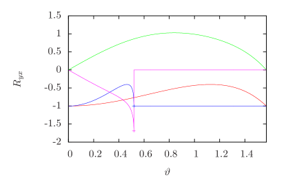
Figure 1: The different reflection coefficients as a function of the angle of incidence $\vartheta$. $R_{PP}$ (red line), $R_{SP}$ (green line), $R_{SS}$ (blue line), $R_{PS}$ (pink line). Note, $R_{yx}$ means incident $x$-wave and reflected $y$-wave.

Following Ach73 , when a plane elastic wave hits a free surface, we first define a reflection plane. This is the plane spanned by the surface normal and the propagation direction of the ray. An incident $P$-wave splits into an out-going $P$-wave and an out-going $S$-wave with polarization vector lying in the plane of reflection. The reflection amplitudes for both waves are given by:

$$R_{PP} =\frac{\sin(2\vartheta)\,\sin(2\Theta)-\kappa^{2}\,\cos^{2}(2\Theta)}{\sin(2\vartheta)\,\sin(2\Theta)+\kappa^{2}\,\cos^{2}(2\Theta)}\;,\quad\kappa=\frac{\sin\vartheta}{\sin\Theta}$$ (2)

$$R_{SP} =\frac{2\kappa\,\sin(2\vartheta)\,\cos(2\Theta)}{\sin(2\vartheta)\,\sin(2\Theta)+\kappa^{2}\,\cos^{2}(2\Theta)}\;,$$ (3)

where $\kappa=c_{d}/c_{s}>1$ such that the exit angle $\Theta$ is always smaller than the entrance angle $\vartheta$. These angles are always measured with respect to the normal of the surface. The reflection amplitudes $R_{PP}$ and $R_{SP}$ determine the amplitudes of the two out-going waves.

The case of an incident $S$-wave is more complicated. Before considering the reflection itself, we have to decompose the wave into one component with polarization in the reflection plane (SV-wave) and another with polarization perpendicular to it (SH-wave). For the SV-wave we then have similar reflection coefficients as for the $P$-wave:

$$R_{SS} =\frac{\sin(2\vartheta)\,\sin(2\Theta^{\prime})-\kappa^{2}\,\cos^{2}(2\vartheta)}{\sin(2\vartheta)\,\sin(2\Theta^{\prime})+\kappa^{2}\,\cos^{2}(2\vartheta)}\;,\quad\kappa=\frac{\sin\Theta^{\prime}}{\sin\vartheta}$$ (4)

$$R_{PS} =\frac{-\,\kappa\,\sin(4\vartheta)}{\sin(2\vartheta)\,\sin(2\Theta^{\prime})+\kappa^{2}\,\cos^{2}(2\vartheta)}\;,$$ (5)

where now $\Theta^{\prime}>\vartheta$ such that these equations only apply as long as $\kappa\sin\vartheta<1$. This introduces the critical angle (of incidence) $\vartheta_{\rm cr}=\arcsin(\kappa^{-1})$. However, for SV-waves incident at larger angles, the reflected P-wave becomes a surface wave with negligible contribution to the wave field, while the reflection amplitude for the SV-wave becomes

$$R_{SS}=-\;\frac{\cos^{2}(2\vartheta)-2{\rm i}\,\beta\,\sin\vartheta\,\sin(2\vartheta)}{\cos^{2}(2\vartheta)+2{\rm i}\,\beta\,\sin\vartheta\,\sin(2\vartheta)}\;,$$ (6)

where $\beta=\sqrt{\sin^{2}\vartheta-\kappa^{-2}}$. The absolute value squared of $R_{SS}$ is one in that case, which means that all the energy is transferred to the reflecting $S$-wave.

SH-waves, i.e. shear waves with polarization direction perpendicular to the reflection plane, cannot convert to $P$-waves. They are reflected according to the standard law where the reflection angle is equal to the angle of incidence.

II.2 Classical ray limit

In order to define the classical ray limit, we consider a localized wavepacket of total energy $Q$. At any moment in time this wavepacket has a well defined position $\vec{r}$ and propagation direction $\vec{\rm e}_{v}$. With respect to its momentary position $\vec{r}$, the wavepacket has a certain extension along the propagation direction and perpendicular to it. Typically, we would imagine a cigar-shaped wavepacket, oriented along the propagation direction. In the classical limit, we ignore the transversal extension of the wavepacket and obtain thereby a one dimensional object. For the studies to follow, the wavepacket’s extension along the propagation direction does not matter. Since elastic waves propagate in two different modes, the classical description must be extended by some internal variables: We need one binary variable to specify the mode of the wavepacket which may be longitudinal ($P$) or transversal ($S$). Moreover, if the wavepacket is in transversal mode, we need to record the polarization direction by a unit vector $\vec{\rm e}_{p}$, perpendicular to the propagation direction.

The classical description of elastic waves runs into difficulties when it comes to reflections. The problem is ray splitting KohBlu98 , which will be treated as follows: We assume that in the vicinity of the wavepacket center, an elastic ray may be described as a plane wave. For that plane wave, the reflection laws of the previous section II.1 apply. As explained there, the reflected wave will in general be split into an $S$-mode and a $P$-mode branch, propagating into different directions. Accordingly, the reflected ray splits in two, where the local intensities and polarization directions in the wavepacket center may be calculated from the reflection coefficients of the corresponding plane waves. Finally, purely geometric considerations allow to determine the widths of those branches. In that way, we obtain the complete information about the two reflected branches of the incident ray. Note that an incident $S$-mode ray must be considered as a linear combination of a $SV$-wave (polarization direction in the reflection plane) and a $SH$-wave (polarization direction perpendicular to the reflection plane). Hence, the $P$-wave branch of the reflected ray is obtained solely from the $SV$ component, wheras the $S$-wave branch is given as a superposition of the reflected $SH$-wave and the $S$-wave branch of the $SV$-component. These relations explain why it is necessary to keep track of the polarization direction of the $S$-mode rays.

For the classical description of the secondary rays, we need neither the wavepacket-widths nor the local intensities, however, we do need the total energy share of each branch. In principle, the calculation of the total energy share is rather involved since it requires the integration of the energy flux across a surface perpendicular to the propagation direction, taking into account the variation of the wavepacket intensity. Fortunately, for the reflected branch without mode conversion, neither the wavepacket’s intensity profile nor its propagation speed change. As a consecuence, the total energy contained in that branch is simply proportional to the intensity calculated from the corresponding reflection coefficients:

• An incident $P$-wave carrying the energy $Q$ will transfer the energy $R_{PP}^{2}\,Q$ to the reflected $P$-mode branch.

• An incident $S$-wave of the same energy whose polarization direction makes an angle $\theta$ with the reflection plane must be split into the $SV$-component of energy $Q_{V}=Q\,\cos^{2}\theta$ and the $SH$-component of energy $Q_{H}=Q\,\sin^{2}\theta$. The total energy of the reflected $S$-mode branch then is $R_{SS}^{2}\,Q_{V}+Q_{H}$.

Energy conservation now implies that the respective mode-converted branch must carry the remaining energy. That this is indeed the case, is shown exemplarily for an incident $P$-mode ray in the appendix.

Returning to the propagation of the elastic ray, we note that subsequent reflections lead to further subdivisions into an exponentially increasing number of branches. Topologically, an elastic ray may be considered as a tree, where the initial energy is transported from the trunk towards the outer (higher order) branches. Even for modest travel times, it is soon impossible to keep track of all the branches of the elastic ray.

We therefore employ a Monte Carlo method to sample implicitely only over those branches which carry the largest amount of energy. For that purpose we translate energy share into probability. Thus, we replace the deterministic energy distribution model by a statistical model, where we define an ensemble of rays which all start in the same initial state corresponding to a wave packet with energy $Q_{0}$. At each reflection, we choose at random, whether the ray follows one branch or the other. The probability with which one option or the other is chosen, are simply given by the relative energy shares calculated from the corresponding reflection coefficients. At the end, the probability to travel through a certain higher order branch is given by the product of probabilities for the choices made along the history of the given ray. This probability agrees with the energy ratio between the total energy of the wavepacket in that particular branch and the energy of the initial wavepacket. Thus, in a numerical simulation, the energy share of a higher order branch can be estimated from the number of members in the ensemble which terminate in that given branch.

Our ensemble of rays may as well start in different initial states also chosen at random. That is the case, when we intend to calculate the evolution of a statistical ensemble of initial conditions. In what follows, we will consider the following three different types of initial conditions:

• Deterministic initial conditions, where we completely specify one particular ray, starting at a certain point, in a specific direction, either in $S$- or $P$-mode, and in case with a specific polarization.

• Surface initial conditions, where we start $P$-waves at a particular point on the surface of the body, while the direction of the ray is chosen at random within the half sphere pointing into the body.

• Homogeneous initial conditions, where we start rays at random positions inside the body, with random directions (isotropic on the whole unit sphere) in $S$- or $P$-mode with probabilities chosen according to the equipartition ratio in Eq. (7) and in case random polarization direction.

III Random mode conversion model

In Ref. LobWea03 the authors introduce a simple model, ignoring any geometric effects, where elastic rays undergo random and statistically independent mode conversions according to the conversion rates $\alpha$ ($S$-to-$P$) and $\beta$ ($P$-to-$S$). Here, the mean free time between two conversions is given by $\alpha^{-1}$ (for the $S$-mode segments) and $\beta^{-1}$ (for the $P$-mode segments), respectively. As an additional ingredient, the authors invoke the equipartition principle, which states that energy should be distributed equally among the different degrees of freedom. Taking into account the different wave speeds for $P$- and $S$-mode waves, the ratio of the energy share between $S$- and $P$-mode waves is Wea82

$$R=2\;\left(\frac{c_{d}}{c_{s}}\right)^{3}\;.$$ (7)

This number also determines the ratio between the conversion rates, since the equilibrium condition of the corresponding rate equation demands that on average, the number of elastic rays in $P$-mode and $S$-mode are related by

$$\frac{\langle N_{S}\rangle}{\langle N_{P}\rangle}=\frac{\beta}{\alpha}=R\;.$$ (8)

One last piece of information is necessary in order to be able to estimate the values of the conversion rates. The authors obtain this from an analogy to room acoustics Pierce1981 and a detailed calculation of the mode conversion probability during individual reflections Graff1991 . The result is:

$$\beta=0.59\;c_{d}\;\frac{S}{4V}\;.$$ (9)

In order to explain the experiments performed on the various Aluminum samples, one requires the statistics of $t_{P}$, the accumulated amount of time a given ray of duration $t$ spends in $P$-mode. As an estimate for the mean $\langle t_{P}\rangle$ and its variance ${\rm var}(t_{P})$ the authors find

$$\langle t_{P}\rangle=\frac{t}{R+1}\;,\qquad{\rm var}(t_{P})=\frac{2t}{\beta}\;\frac{R^{2}}{(1+R)^{3}}\;.$$ (10)

The first equation is easily explained on the basis of ergodicity. A more involved calculation is required for the second.

For Fig. 2 we performed numerical simulations for the random mode conversion model described above. We use random numbers with exponential probability densities to generate sequences of alternating $P$- and $S$-mode time segments forming a random realisation of an elastic ray. With the total time $t$ being fixed we can than measure the average $P$-mode occupation time $\langle t_{P}\rangle$ as well as its variance. These quantities are shown in Fig. 2 as a function of $t$, for three different cases: When the trajectory starts with a $P$-mode segment, with a $S$-mode segment, or by choosing $P$-mode or $S$-mode at random acording to the equipartition ratio. We find that in all cases, $\langle t_{P}\rangle$ and ${\rm var}(t_{P})$ quickly converge to the theoretical values as $t$ becomes sufficiently large.

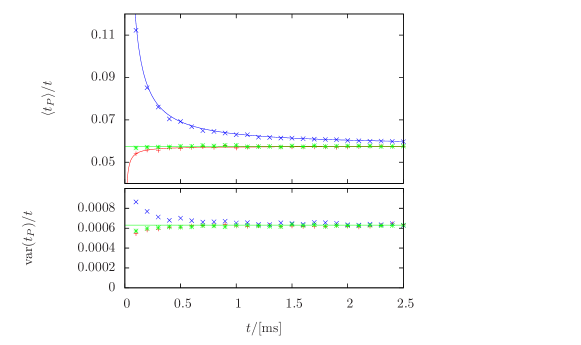
Figure 2: Mean and Variance of the $P$-mode travel time for the Lobkis’ and Weavers’s random conversion model. The $P$-to-$S$-conversion rate was chosen as $\beta=162$. The different colors refer to different initial conditions: starting in $S$-mode (red), starting in $P$-mode (blue), starting randomly in $S$- or $P$-mode according to the equipartition ratio (green). In the case of the equipartitioned initial condition, the solid green line shows the value of the theoretical expectation, Eq. (10). Other solid lines (red and blue) show simple rational best fit functions to guide the eye.

IV Numerical results

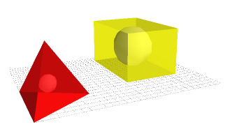
Figure 3: On left a regular tetrahedron with length of 10 cm with inner sphere radius 1.2 cm on right a rectangular block with length of 9 cm width of 13 cm and height of 7.6 cm with inner sphere radius 3.5 cm.

In our simulations we use bodies of two different shapes, a rectangular block of dimensions $9\,{\rm cm}\times 13\,{\rm cm}\times 7.6\,{\rm cm}$ (giving rise to integrable or possibly pseudo-integrable dynamics) and a regular tetrahedron with edges of length $10\,{\rm cm}$, where the dynamics is probably ergodic. In addition, we study each of the two bodies with and without an internal sphere. That sphere is suposed to provide another free surface for the waves (rays) moving inside the body, which renders the dynamics chaotic. The inner sphere for the rectangle is chosen to be relatively large in order to reduce bouncing ball orbits. The bodies (including the inner spheres) are depicted in Fig. 3. According to the random mode conversion model, the volume and the surface area of the bodies are important parameters. These are given in table 1.

As explained earlier, the simulation of the classical rays is done by launching a large number of rays (up to $4\times 10^{6}$) with different initial conditions. Those are chosen to be either of type (ii) (Surface) or of type (iii) (Homogeneous). The former might be considered as corresponding to the experimental situation in Ref. LobWea03 ; LobWea08 , but if at all this may be true only qualitatively.

Body	Volume $[cm^{3}]$	Surface $[cm^{2}]$
Rectangular block	$889.2$	$568.4$
…with inner sphere	$709.6$	$722.3$
Regular tetrahedron	$117.8$	$173.2$
…with inner sphere	$110.6$	$191.3$

Table 1:

IV.1 Conversion rates and equipartition ratio

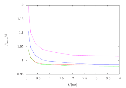
Figure 4: The conversion rate $\beta_{\rm num}$ divided by the travel time $t$, determined from the mean free $P$-mode occupation time, as a function of $t$, for homogeneous initial conditions, for all four different geometries. Tetrahedron with sphere (red line), without sphere (green line), Rectangle with sphere (blue line), and without sphere (pink line).

To verify the accuracy of the random conversion model outlined above, we start by analysing the conversion rates. For that purpose we perform simulations where the initial conditions of the rays are chosen according to the expected equilibrium state. Thus, we start rays at random positions inside the body, with random directions, in $S$- or $P$-mode according to the theoretical equipartition ratio (7), and if in $S$-mode we choose the polarization direction also at random. For each ray of pre-defined duration $t$, we then record all periods during which the ray happened to travel in $P$-mode. The average over those periods over all rays is just the mean free $P$-mode travel time, and therefore equal to $\beta^{-1}$. In Fig. 4 the so determined conversion rate $\beta_{\rm num}$ is compared to the theoretical estimate (9) for all four geometries considered. We find that as soon as $t$ is large enough (for the random mode conversion model to become valid, there need to occur sufficiently many reflections), $\beta_{\rm num}$ is quite close to the theoretical estimate. In fact, as can be observed in Fig. 4, $\beta_{\rm num}$ never deviates more than $3\%$ from the theoretical estimate. Nevertheless, there are systematic differences for the different geometries. While $\beta_{\rm num}$ ends up about $2\%$ above the theoretical estimate in the case of the rectangular block with inner sphere, $\beta_{\rm num}$ ends up about $3\%$ below, in the other three cases. We believe that this behavior is still acceptable in view of the fact that Eq. (9) relies on rather rough estimates.

IV.1.1 Equipartition ratio

In the Figs. 5 and 6, we study the energy share between $S$- and $P$-mode rays. Since our simulations assume an equal amount of energy associated with each ray, that energy share can be computed from the relative frequencies with which we find a particular realization of the rays in either one of the two possible modes. In Figs. 5 and 6, we plot the ratio of these frequencies vs. $t$, the travel time.

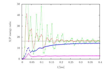
Figure 5: S-mode vs. P-mode energy ratio for samples of different geometries. Rays are started on the surface in $P$-mode with random directions (Surface type initial conditions). The color coding for the different geometries is the same as in Fig. 4. The black horizontal line shows the equipartition ratio $R$, according to Eq. (7).

In Fig. 5 the simulation always starts with initial conditions on the surface [initial conditions of type (ii)], where we applied the Monte Carlo sampling with $4\times 10^{5}$ random realizations, for each of the four different geometries. Theoretically, we expect that the $S/P$ energy ratio converges to $R=$ as given in Eq. (7). Since in the present case, the rays always start in $P$-mode, the energy ratio at small times is close to zero. We observe that two tetrahedrons show a similar behavior, which is very distinct from that of the two rectangular blocks. They approach the theoretical value for $R$ via damped irregular oscillations which are initially very strong. Comparing the two tetrahedrons, the presence of the inner sphere, tends to reduce the strength of the oscillations such that the theoretical value for $R$ is reached faster. By contrast, the rectangular blocks show almost no oscillations at all, and quickly go over to a smooth approach of different limit values for the energy ratio. In doing so, the rectangle with inner sphere comes much closer to the theoretical value for $R$ than the rectangle without inner sphere.

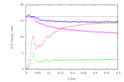
Figure 6: S-mode vs. P-mode energy ratio for the rectangular block with and without internal sphere. The initial conditions were chosen homogeneous and isotropic (blue and pink line) and starting from a fixed point on the surface (always starting in $P$-mode) (red and green line). The black horizontal line shows the value of the equipartition ratio $R$, Eq. (7).

Fig. 6 shows simulations for the two rectangular blocks with initial conditions of type (ii) (on the surface) and type (iii) (homogeneous). At small times, the energy ratio shown starts at zero for initial conditions on the surface, and at the value of the equipartition ratio $R$, for homogeneous initial conditions. As $t$ increases, the curves first show some minor fluctuations and then start to converge to different equilibrium values – in all cases clearly below the equipartition ratio. For the rectangular block with inner sphere, we observe that independent of the type of initial conditions, the energy ratio converges to the same equilibrium value. For the rectangle without inner sphere, this is not the case, and the equilibrium values a very different.

Extending these simulations up to times of the order of $5\,{\rm ms}$, we have confirmed that the $S/P$-energy ratio converges to finite values in the limit of large times, except for the rectangular block without inner sphere. Surprisingly, we have found that these values do not depend on the type of initial conditions applied (Surface or Homogeneous). Concretely, we found the following values:

$$R=\left\{\begin{array}[]{rcl}16.538&:&\text{Tetrahedron without sphere}\\ 16.308&:&\text{Tetrahedron with sphere}\\ 14.685&:&\text{Rectangle with sphere}\\ 9.5/3.2&:&\text{Rectangle without sphere}\end{array}\right.\;,$$ (11)

while the theoretical value is $R=16.384$. We can see that the rectangular block without inner sphere must be considered separately. Only in that case does the equilibrium distribution of the energy share depend on the initial state (for homogeneous initial conditions we get $R=9.5$, otherwise $R=3.2$).

IV.2 P-mode occupation time statistics

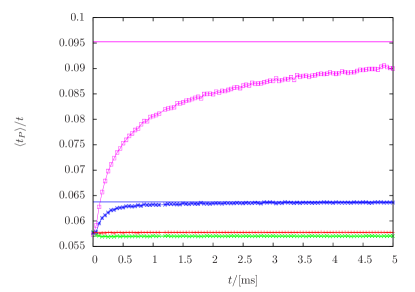
Figure 7: For homogeneous initial conditions, the mean $P$-mode occupation time $\langle t_{P}\rangle$ for the different geometries, divided by the total travel time $t$. We compare with the theoretical estimate, Eq. (10), where we have inserted the numerical values given in Eq. (11). The color coding is as before: Tetrahedron with inner sphere (red points), without inner sphere (green points), Rectangular block with inner sphere (blue points), without inner sphere (pink points). The corresponding estimates for the asymptotic value are depicted as horizontal lines of the same color.

In this section, we restrict ourselves to homogeneous initial conditions. In our simulations, every trajectory at each reflection makes a random choice whether to do a mode conversion or not. This results in different trajectory paths and different amounts of times, the ray spends in each mode. In what follows, we study the distribution of the $P$-mode occupation time $t_{P}$; obviously, the corresponding $S$-mode occupation time would provide exactly the same information. We have chosen this particular quantity because it may be linked to experimental results in LobWea03 ; LobWea08 with the theoretical models proposed in Sni06 (Coda wave interferometry) and LobWea03 (random mode conversion model).

We start with the average $P$-mode occupation time $\langle t_{P}\rangle$, for which the random mode conversion model makes the prediction (10). In Fig. 2(a) we have seen that this prediction is indeed very accurate, provided the ensemble of rays is in the standard equilibrium state. Fig. 7 shows $\langle t_{P}\rangle/t$ for homogeneous initial conditions which according to theory should converge to $(1+R)^{-1}$ at sufficiently large times. Indeed for the tetrahedron as well as the rectangle with inner sphere, the prediction is fulfilled. The ratio $\langle t_{P}\rangle/t$ converges to the predicted value, if we replace the theoretical equipartition ratio with the one obtained numerically from our simulations (these values are given in Eq. (11)). In the case of the rectangle without inner sphere (out of range), the convergence of $\langle t_{P}\rangle/t$ is much slower but the limit value still consistent with the numerical $S/P$ energy partitioning.

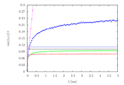
Figure 8: For homogeneous initial conditions, the variance of the $P$-mode occupation times for the different geometries, rescaled by $\beta/t$. The color coding for the different geometries is the same as in Fig. 7. We compare with the theoretical estimate, Eq. (10), where $\beta$ has dropped out (black horizontal line). Correcting the theoretical expectation for the $\beta$-values observed in Fig. 4, leads to the blue horizontal line for the rectangular block with inner sphere.

Fig. 8 shows the variance of the $P$-mode occupation times, divided by $t/\beta$ with $\beta$ calculated from Eq. (9). The black solid horizontal line shows the theoretically expected value according to the random mode conversion model (10), where $\beta$ drops out (black horizontal line):

$${\rm var}(t_{P})\;\frac{\beta}{t}\;\to\;\frac{2R^{2}}{(1+R)^{3}}\approx 0.1022\;.$$ (12)

Correcting the theoretical expectation for the numerically determined $\beta$-values shown in Fig. 4 does not make a noticeable difference in the case of the Tetrahedrons and leads to the blue horizontal line for the rectangular block with inner sphere. In the case of the rectangular block without sphere, we find a steep linear increase of ${\rm var}(t_{P})\,\beta/t$, such that a comparison with a theoretical limit value makes no sense.

In this last figure we find the largest deviations from the random mode conversion model. The result for the tetrahedron with sphere is about $25\%$ below the theoretical value; without sphere, it is about $5\%$ below, while the result for the rectangle with sphere is more than $100\%$ above the theoretical value. The result for the rectangle without sphere is totally off the scale.

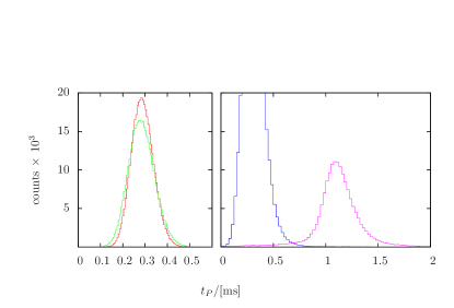
Figure 9: For homogeneous initial conditions, the histograms for the $t_{P}$ statistics for $t=5\,{\rm ms}$. The result for the tetrahedrons on the left, with/without inner sphere (red/green solid line); for the rectangular blocks on the right with/without inner sphere (blue/pink solid lines).

Finally, we show in Fig. 9 the distribution of $P$-mode occupation times $t_{P}$ for trajectories of duration $t=5\,{\rm ms}$. In the case of the tetrahedrons, we find that the distributions are close to Gaussians, with the distribution for the tetrahedron with inner sphere being a bit narrower than for the tetrahedron without. In the case of the rectangular blocks, the distributions are clearly non-Gaussian. For the rectangle with inner sphere the distribution is strongly asymmetric, while for the rectangle without inner sphere, the distributions is surprisingly close to a Lorentzian. This latter observation can explain the fact that the variance of the $P$-mode occupation times scales with $t^{2}$ rather than $t$, since the variance of a Lorentzian distribution is infinite.

V Discussion

V.1 Related experimental results

In Refs. LobWea03 ; LobWea08 , the authors measured the acoustic long time response of short initial ultrasound pulses applied to different Aluminum bodies. They studied the cross correlations between these signals taken at different temperatures. Since the temperature change induces a change of the propagation speeds of $P$- and $S$-waves by different amounts, a temperature change results in the distortion of the acoustic signal and a reduction of the cross correlations. The reduction of the cross correlations, which has also been identified as a scattering fidelity SGSS05 ; SSGS05 ; GPSZ06 , can be described quantitatively within the theory of Coda wave interferometry Sni06 .

As this theory shows, scattering fidelity (or “distortion” how that quantity has been called in Ref. LobWea03 ) is essentially given by the distribution of $P$-mode occupation times – the quantity studied in the previous Sec. IV.2. Assuming Gaussian statistics for these times, the scattering fidelity or distortion may be related to the variance of the $P$-mode occupation times as follows:

$$D(t)=2\pi^{2}\;(\Delta T\,f)^{2}\;(\delta_{p}-\delta_{S})^{2}\;{\rm var}(t_{p})\;,$$ (13)

where $f$ is the carrier frequency of the elastic wave, $\Delta T$ is the change in temperature, while $\delta_{P}=-1.685\times 10^{-4}\,{\rm K}^{-1}$, and $\delta_{S}=-2.9\times 10^{-4}\,{\rm K}^{-1}$ are the thermal dilation coefficients for $P$-waves and $S$-waves, respectively LobWea03 .

In Ref. LobWea03 , Lobkis and Weaver measured the slope of $D(t)$ scaled by $\Delta T^{2}$, $f^{2}$ and $\beta^{-1}$, which according to the random mode conversion model should always be the same. For our simulations, this is equivalent to determining the slope of ${\rm var}(t_{P})$ as a function of time, scaled by $\beta^{-1}$, which should then also give a unique value; see Eq. (12). For the Aluminum blocks of different shapes, analysed in Ref. LobWea03 , the result was a wide spreading of experimental values where, the smallest values roughly agreed with the theoretical expectation, while the largest values where about four times larger . On a qualitative basis, one could observe the tendency that less chaotic geometries lead to larger values for the slope.

V.2 Our results

The overall result of the present analysis, shown in Fig. 8, is similar in this respect. We also find that the slopes can be very different for different geometries. It however shows that the relevant quantity is not really chaos as measured by Lyapunov exponents but possibly rather ergodicity. From the four different geometries considered, the tetrahedron with inner sphere has the smallest slope. It is notable in that case, that the slope is about $25\%$ below the theoretical value, which shows that the theory doesn’t provide a lower bound as one might have been conjectured from the experimental results. Next comes the tetrahedron without inner sphere. Because all its surfaces are plane, the Lyapunov exponent must be zero in any case. However, the tetrahedron has most likely ergodic dynamics. And we find indeed that the slope is quite close to the theoretical expectation. Only at a considerable distance, we find the rectangle with inner sphere. The inner sphere clearly leads to chaotic dynamics with positive Lyapunov exponents, but there are also regions of integrable dynamics and bouncing ball orbits. That is apparently sufficient to increase the slope to more than twice the theoretical value. The rectangle without inner sphere is clearly the most regular body. For that geometry, the ${\rm var}(t_{P})$ curve rather shows a quadratic dependence on $t$. This is in line with the probability density for the $P$-mode occupation times shown in Fig. 9. Its shape is almost a Lorentzian which would imply an infinite variance.

Our simulations have shown that many of the assumptions within the random mode conversion model are rather nicely met. This is true for the $P$-to-$S$ conversion rate $\beta$ (Fig. 4), and also for the equipartition ratio if the dynamics is ergodic (Fig. 5). We could also confirm that the average $P$-mode occupation time is always related to the $S/P$-energy ratio (Fig. 7). Thus, the weak point of the random mode conversion model is clearly the in general inaccurate or wrong prediction of the variance of the $P$-mode occupation times. This shows that the succession of $P$-mode and $S$-mode segments is in general not well described by a Poissonian process. We believe that there are two effects coming into play. (i) The duration of the individual $P$-mode segments (these are the shortest ones) cannot be really exponentially distributed because the rays have to travel a certain distance before having the possibility to undergo a mode conversion. (ii) The durations of subsequent $P$-mode and $S$-mode segments might be correlated.

The first effect would lead to a smaller variance of the duration of the $P$-mode segments and thereby to a smaller variance of the total $P$-mode occupation times. Thus if the dynamics destroys correlations sufficiently rapidly, ${\rm var}(t_{P})$ should be smaller than expected theoretically. Our findings suggest that this is indeed the case for the tetrahedron with inner sphere. The tetrahedron without inner sphere is ergodic but needs more time to destroy correlations. It thus seems that the second effect related to correlations tends to enlarge ${\rm var}(t_{P})$. For the rectangle with inner sphere, correlations are not efficiently destroyed and the variance of the $P$-mode occupation times becomes much larger still. At last, we have the rectangle without inner sphere, where ${\rm var}(t_{P})$ scales with $t^{2}$.

VI Conclusions

We presented simulations of the propagation of elastic waves in three-dimensional bodies of different geometries in the limit of classical rays. Because of mode conversion at the reflections on the surface of the bodies, one has to deal with an exponential proliferation of branches of the elastic ray, which is dealt with using Monte Carlo sampling.

Our simulations have shown that there is no unique universal equilibrium distribution for elastic rays, at least not for bodies with a sufficiently simple geometry. This is true even if the dynamics must be considered as completely chaotic. For the tetrahedron with internal sphere, the equilibrium limit of the $S/P$ energy ratio was close but not exactly equal to the theoretical value. Even more surprisingly, we found that the homogeneous and isotropic distribution of elastic rays with an $S/P$ energy ratio equal to the theoretical equipartition ratio need not be an equilibrium distribution at all. When chosen as the initial condition of an ensemble of elastic rays, we found that in the case of the rectangular blocks, the $S/P$ energy ratio changes to a different value.

The main purpose of the present work was to analyse some of the conjectures made in Ref. LobWea03 and to investigate, whether the observed deviations can be explained with a model based on classical rays. While many conjectures and approximations were indeed justified, the most problematic assumption was that of random mode conversions with given conversion rates. There, we found two counteracting effects: One the one hand the length distribution of individual $P$-mode and $S$-mode segments is not exponential due to the fact that mode conversions can take place only during reflections. On the other hand, there are correlations in time where the time scale depends on the dynamics. In comparison to the random mode conversion model, the former tends to reduce the variance of the $P$-mode occupation time while the latter leads to an increase.

Previous publications GSW06 ; LobWea08 have focused on the form of the decay function of scattering fidelity which has been shown to follow very closely universal random matrix predictions. However, our results indicate that the perturbation strength is an equally interesting quantity. In fact it reveals much more system specific information, which may even have practical applications, for example in the analysis and verification of the properties of mechanical components. It would be interesting to design new experiments, which allowed for a quantitative comparison between experiment and numerical simulations.

Appendix A Energy conservation during ray splitting

In Sec. II.2, we discuss the splitting of the total energy of a reflected wavepacket in the ray limit. In order to determine the energy share of the mode-converted branch, we assumed energy conservation, which is an important issue for the self-consistency of our ray model. It implies that the reflection coefficients defined in Eqs. (2-6) are related. Here, we show exemplarily for an incident ray in $P$-mode that the total energy is indeed conserved.

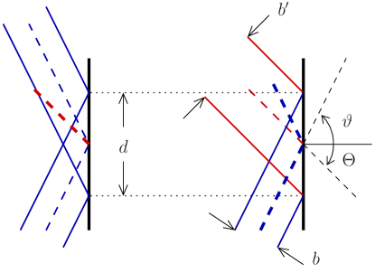
Figure 10: Transformation of the ray widths under mode conversion. If the exit angle is equal to the angle of incidence (no mode conversion), the width of the reflected ray is unchanged. Otherwise the widths are proportional to the cosines of the angles $\vartheta$ and $\Theta$.

The amplitude of an elastic ray is physically related to the displacement of infinitesimal volume elements in the solid. Therefore, amplitudes $u_{P}$ or $u_{S}$ (for $P$-mode and $S$-mode, respectively) have units of length. The period averaged energy density of the respective wave field is then given by

$${\varepsilon}_{P,S}=\frac{\varrho\,w^{2}}{2}\;u_{\{P,S\}}^{2}\;,$$ (14)

where $\varrho$ is the density of the medium and $w$ the angular frequency of the wave (see Sec. 1.7 of Ach73 ). To demonstrate the energy conservation, we show that the energy flux is conserved in a quasi-stationary situation where a very long wave packet is reflected at a free plane surface. It means that the energy flux along the propagation direction of the incident $P$-mode ray must be equal to the sum of the fluxes along the reflected $P$-mode and the reflected and mode-converted $S$-mode branch: In general, the amount of energy flowing through a transversal surface $S$ is given by

$$F=\int_{S}{\varepsilon}(\vec{r})\;v_{n}(\vec{r})\;{\rm d}\sigma(\vec{r})\;,$$ (15)

where $v_{n}$ is the projection of the ray velocity on the surface normal. If we choose $S$ to be normal to the propagation direction:

$$F_{P/S}=\frac{\varrho\,w^{2}}{2}\;c_{d/s}\int_{S}u_{P/S}(\vec{r})^{2}\;{\rm d}\sigma(\vec{r})\;.$$ (16)

Just as the propagation speed, also the energy flux depends on the wave mode. Now, if the energy flux is really conserved, the following relation must hold:

$$\frac{\varrho w^{2}}{2}\;c_{d}\int_{S}u_{P}(\vec{r})^{2}\;{\rm d}\sigma(\vec{r})=\frac{\varrho w^{2}}{2}$$

$$\times\left[c_{d}\;R_{PP}^{2}\int_{S^{\prime}}u_{P}^{\prime}(\vec{r})^{2}\,{\rm d}\sigma(\vec{r})+c_{s}\;R_{SP}^{2}\int_{S^{\prime\prime}}u_{P}^{\prime\prime}(\vec{r})^{2}\,{\rm d}\sigma(\vec{r})\right]$$

(17)

where $S$ is a surface perpendicular to the incident ray, $S^{\prime}$ is a surface perpendicular to the reflected $P$-mode branch and $S^{\prime\prime}$ is a surface perpendicular to the reflected $S$-mode branch. We have assumed that these surfaces are sufficiently to the reflection point such that the wave amplitudes may be considered constant along the line segments towards and away from the reflection point. The reflection is schematically depicted in Fig. 10 separately for the $P$-mode branch (left hand side) and the $S$-mode branch (right hand side). Without mode conversion, the geometrical properties of the ray do not change, such that the amplitude $u_{P}^{\prime}$ relative to $S^{\prime}$ is just equal to $u_{P}$ relative to $S$, which means that the corresponding integrals coincide. With mode conversion, the width of the ray increases by the factor $\cos\Theta/\cos\vartheta>1$. Thus, the integral over $S^{\prime\prime}$ must be scaled by that factor. Therefore, dividing by the common factor $\varrho w^{2}/2$,

$$c_{d}\;(1-R_{PP}^{2}) \int_{S}u_{P}(\vec{r})^{2}\;{\rm d}\sigma(\vec{r})=c_{s}\;R_{SP}^{2}\;\frac{\cos\Theta}{\cos\vartheta}$$ (18)

$$\qquad\times\int_{S}u_{P}(\vec{r})^{2}\;{\rm d}\sigma(\vec{r})$$

Now, since the integrals are the same, we arrive at

$$1-R_{PP}^{2}=\frac{c_{s}}{c_{d}}\;R_{SP}^{2}\;\frac{\cos\Theta}{\cos\vartheta}\;,$$ (19)

which may be easily verified. Thus the energy flux is indeed conserved.

References

- (1) R. Snieder, Pure appl. geophys. 163, 455 (2006)
- (2) R. Courtland, Nature 453, 146 (2008)
- (3) E. Larose, J. De Rosny, L. Margerin, D. Anache, P. Gouedard, M. Campillo, and B. van Tiggelen, Phys. Rev. E 73, 016609 (2006)
- (4) A. Kohler and R. Blümel, Ann. Phys. 267, 249 (1998)
- (5) M. V. Berry, Proc. R. Soc. Lond. A 400, 229 (1985)
- (6) P. Jacquod, P. G. Silvestrov, and C. W. J. Beenakker, Phys. Rev. E 64, 055203(R) (2001)
- (7) N. R. Cerruti and S. Tomsovic, Phys. Rev. Lett. 88, 054103 (2002)
- (8) O. I. Lobkis and R. L. Weaver, Phys. Rev. Lett. 90, 254302 (2003)
- (9) R. Schäfer, T. Gorin, H.-J. Stöckmann, and T. H. Seligman, New J. Phys. 7, 152 (2005)
- (10) R. Schäfer, H.-J. Stöckmann, T. Gorin, and T. H. Seligman, Phys. Rev. Lett. 95, 184102 (2005)
- (11) T. Gorin, T. H. Seligman, and R. L. Weaver, Phys. Rev. E 73, 015202(R) (2006)
- (12) T. Gorin, T. Prosen, T. H. Seligman, and M. Žnidarič, Phys. Rep. 435, 33 (2006)
- (13) O. I. Lobkis and R. L. Weaver, Phys. Rev. E 78, 066212 (2008)
- (14) R. L. Weaver, J. Acoust. Soc. Am. 71, 1608 (1982)
- (15) A. D. Pierce, Acoustics: An Introduction (McGraw-Hill, 1981)
- (16) K. F. Graff, Wave Motion in Elastic Solids (Dover, 1991)
- (17) H. Schomerus and P. Jacquod, J. Phys. A: Math. Gen. 38, 10663 (2005)
- (18) M. C. Gutzwiller, Chaos in classical and quantum mechanics (Springer, 1990)
- (19) L. Kaplan, New J. Phys. 4, 90 (2002)
- (20) E. Bogomolny, N. Pavloff and C. Schmit, Phys. Rev. E 61, 3689 (2000)
- (21) J. S. Hersch, M. R. Haggerty and E. J. Heller, Phys. Rev. E 62, 4873 (2000)
- (22) J. D. Achenbach, Wave propagation in elastic solids, Applied mathematics and mechanics, Vol. 16 (North-Holland, 1973)
- (23) Ignoring the case of a regular cylinder, which has been off the scale.