Roots of random polynomials whose coefficients have logarithmic tails

Abstract

It has been shown by Ibragimov and Zaporozhets [In Prokhorov and Contemporary Probability Theory (2013) Springer] that the complex roots of a random polynomial $G_{n}(z)=\sum_{k=0}^{n}\xi_{k}z^{k}$ with i.i.d. coefficients $\xi_{0},\ldots,\xi_{n}$ concentrate a.s. near the unit circle as $n\to\infty$ if and only if ${\mathbb{E}\log_{+}}|\xi_{0}|<\infty$. We study the transition from concentration to deconcentration of roots by considering coefficients with tails behaving like $L({\log}|t|)({\log}|t|)^{-\alpha}$ as $t\to\infty$, where $\alpha\geq 0$, and $L$ is a slowly varying function. Under this assumption, the structure of complex and real roots of $G_{n}$ is described in terms of the least concave majorant of the Poisson point process on $[0,1]\times(0,\infty)$ with intensity $\alpha v^{-(\alpha+1)}\,du\,dv$.

and

1 Introduction and statement of results

1.1 Introduction

Let $\xi_{0},\xi_{1},\ldots$ be i.i.d. nondegenerate random variables with values in $\mathbb{C}$. Let $\mathcal{Z}_{n}$ be the collection of complex roots (counted according to their multiplicities) of the random polynomial

$$G_{n}(z)=\sum_{k=0}^{n}\xi_{k}z^{k}.$$ (1)

For $0\leq a\leq b$ denote by $R_{n}(a,b)$ the number of roots of $G_{n}$ in the ring $\{z\in\mathbb{C}\dvtx a\leq|z|\leq b\}$. Improving on a result of Šparo and Šur sparosur , Ibragimov and Zaporozhets izlog show that

$$\frac{1}{n}R_{n}(1-\varepsilon,1+\varepsilon)\mathop{\longrightarrow}_{n\to\infty}^{\mathrm{a.s.}}1$$ (2)

for every $\varepsilon\in(0,1)$, if and only if

$${\mathbb{E}\log_{+}}|\xi_{0}|<\infty.$$ (3)

Here, $\log_{+}x=\max(\log x,0)$. Without any assumptions on the distribution of $\xi_{0}$, Ibragimov and Zaporozhets izlog also prove that for every $\alpha,\beta$ such that $0\leq\alpha<\beta\leq 2\pi$,

$$\frac{1}{n}\sum_{z\in\mathcal{Z}_{n}}\mathbh{1}_{\{\alpha\leq\arg z\leq\beta\}}\mathop{\longrightarrow}_{n\to\infty}^{\mathrm{a.s.}}\frac{\beta-\alpha}{2\pi}.$$ (4)

Thus, under a very mild moment condition, the complex roots of $G_{n}$ concentrate near the unit circle uniformly by the argument as $n\to\infty$.

Imposing additional conditions on the distribution of $\xi_{0}$ it is possible to obtain more precise information about the asymptotic concentration of the roots near the unit circle. In the case when $\xi_{0}$ belongs to the domain of attraction of an $\alpha$-stable law, $\alpha\in(0,2]$, Ibragimov and Zeitouni ibrzeit show that for every $t>0$,

$$\lim_{n\to\infty}\frac{1}{n}\mathbb{E}R_{n}\biggl{(}1-\frac{t}{n},1+\frac{t}{n}\biggr{)}=\frac{1+e^{-\alpha t}}{1-e^{-\alpha t}}-\frac{2}{\alpha t}.$$ (5)

This is a generalization of the result of Shepp and Vanderbei sheppvanderbei who consider real-valued standard Gaussian coefficients.

On the other hand, if ${\mathbb{E}\log_{+}}|\xi_{0}|=\infty$ and thus there is no concentration near the unit circle, it is also possible to describe the asymptotic behavior of the roots when the tail of $|\xi_{0}|$ is extremely heavy. Götze and Zaporozhets goetzezaporozhets prove that if the distribution of ${\log_{+}\log_{+}}|\xi_{0}|$ has a slowly varying tail, then the complex roots of $G_{n}$ concentrate in probability on two circles centered at the origin whose radii tend to zero and infinity, respectively. See also z , zn for more results in the case of extremely heavy tails.

Up to now, the behavior of the roots has been unknown when the tail of $\xi_{0}$ is somewhere between the two cases described above. The aim of this paper is to consider a class of distributions which in some sense continuously links the above cases. We will consider coefficients with logarithmic power-law tails. More precisely, we make the following assumption: for some $\alpha\geq 0$,

$$\quad\bar{F}(t):=\mathbb{P}\bigl{[}{\log}|\xi_{0}|>t\bigr{]}\qquad\mbox{is regularly varying at }{+}\infty\mbox{ with index }{-}\alpha.$$ (6)

This class of distributions includes distributions with both finite ($\alpha>1$) and infinite ($\alpha<1$) logarithmic moments. We will obtain a precise information on how the concentration of the roots near the unit circle becomes destroyed as $\alpha$ approaches $1$ from above and how the roots behave when there is no concentration ($\alpha<1$).

The case $\alpha=+\infty$ corresponds formally to the light or power-law tails studied in sheppvanderbei , ibrzeit . The roots are concentrated near the unit circle and, apart from this, no global organization is apparent. We will prove that as $\alpha$ becomes finite, the distribution of roots becomes highly organized; see Figure 1. The roots “freeze” on a random set of circles centered at the origin. Both the radii of the circles and the distribution of the roots among the circles are random; however, the distribution of the roots on each circle is uniform by the argument. As long as $\alpha$ stays above $1$, the logarithmic moment is finite, and the circles approach the unit circle at rate $n^{1/\alpha-1}$ (ignoring a slowly varying term), in full agreement with the result of izlog . Note also that for $\alpha$ close to $+\infty$, this rate is close to the rate $1/n$ appearing in (5). As $\alpha$ becomes equal to $1$, we have a transition from finite to infinite logarithmic moment. We will show that if $\bar{F}(t)\sim c/t$ as $t\to+\infty$, then the empirical measure formed by the roots of $G_{n}$ converges weakly (without normalization) to a random probability measure concentrated on an infinite number of circles with random radii. For the first time, the roots are not concentrated near the unit circle. As $\alpha$ becomes smaller than $1$, the circles divide into two groups approaching $0$ and $\infty$ at the rates $\pm n^{1/\alpha-1}$, on the logarithmic scale. The number of circles, which was infinite for $\alpha\geq 1$, becomes finite for $\alpha<1$ and decreases to $2$ as $\alpha\to 0$. At $\alpha=0$ the roots freeze on just $2$ circles located very close to $0$ and $\infty$, in accordance with Götze and Zaporozhets goetzezaporozhets , whose results we will strengthen. At $\alpha=0$, the empirical measure formed by the roots becomes almost deterministic: the only parameter which remains random after taking the limit $n\to\infty$ is the proportion of the roots close to $0$ (or to $\infty$), which is uniform on $[0,1]$.

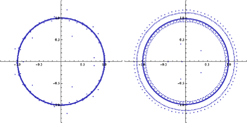
Figure 1: Roots of a random polynomial of degree $n=2000$ whose (real) coefficients are (left) standard normal, (right) such that $\mathbb{P}[\log\xi_{0}>t]=1/t^{2}$ for $t\geq 1$.

An interesting phenomenon we will encounter is the appearance of the long-range dependence between the roots under condition (6). Consider a random polynomial $G_{n}$ of high degree, and suppose that we know that it has a root at some point $z_{0}\in\mathbb{C}$. In the case of coefficients from the domain of attraction of a stable law, this information has almost no influence on the other roots of $G_{n}$, except for the roots located in an infinitesimal neighborhood of $z_{0}$. However, for coefficients with logarithmic power-law tails, the knowledge about the existence of a root at $z_{0}$ implies that there exists (with high probability) a circle of roots containing $z_{0}$. Moreover, the radii of the other circles of roots are influenced by the existence of the root at $z_{0}$. We observe a long-range dependence between the roots: the conditional distribution of roots, given that there is a root at $z_{0}$, differs, even on the global scale, from the unconditional distribution of roots.

If the random variables $\xi_{i}$ are real-valued, we will also analyze the real roots of $G_{n}$. For a particular family of distributions satisfying (6) with $\alpha>1$, Shepp and Farahmand sheppfarahmand show that the expected number of real roots of $G_{n}$ is asymptotically $c(\alpha)\log n$ with $c(\alpha)=\frac{2\alpha-2}{2\alpha-1}$. As $\alpha$ decreases from $+\infty$ to $1$ the function $c(\alpha)$ decreases from $1$ to $0$. We will complement this result by showing that for $\alpha\in(0,1)$, the number of real roots of $G_{n}$ has two subsequential distributional limits as $n\to\infty$ along the subsequence of even/odd integers. This means that for $\alpha\in(0,1)$ the polynomial $G_{n}$ has, roughly speaking, $O(1)$ real roots. Finally, we will prove that for $\alpha=0$, the number of real roots of $G_{n}$ can take asymptotically only the values $0,\ldots,4$ and compute the probabilities of these values.

1.2 Complex roots

Given a complex number $z=|z|e^{i\arg z}$ and $a\in\mathbb{R}$, we write

$$z^{\langle a\rangle}=|z|^{a}e^{i\arg z}.$$

The next theorem describes the structure of complex roots of $G_{n}$. Let $\delta(z)$ be the unit point mass at $z$. Denote by $\bar{\mathbb{C}}=\mathbb{C}\cup\{\infty\}$ the Riemann sphere. We need normalizing sequences $a_{n},b_{n}$ such that

$$\bar{F}(a_{n})\sim\frac{1}{n}\qquad\mbox{as }n\to\infty,\qquad b_{n}=\frac{n}{a_{n}}.$$ (7)

Theorem 1.1

If the tail condition (6) is satisfied with some $\alpha>0$, then we have the following weak convergence of random probability measures on $\bar{\mathbb{C}}$:

$$\frac{1}{n}\sum_{z\in\mathcal{Z}_{n}}\delta\bigl{(}{z^{\langle b_{n}\rangle}}\bigr{)}\mathop{\longrightarrow}_{n\to\infty}^{w}\Pi_{\alpha}.$$

The limiting random probability measure $\Pi_{\alpha}$ is a.s. a convex combination of at most countably many uniform measures concentrated on circles centered at the origin.

Remark 1.2 ((On convergence of random measures)).

Let $E$ be a locally compact metric space. Denote by $\mathbb{M}(E)$ the space of locally finite Borel measures on $E$. Endowed with the topology of vague convergence, $\mathbb{M}(E)$ becomes a Polish space; see resnickbook , Section 3.4. A random measure on $E$ is a random element with values in $\mathbb{M}(E)$. A sequence $\mu_{n}$ of random measures converges weakly to a random measure $\mu$ if $\lim_{n\to\infty}\mathbb{E}F(\mu_{n})=\mathbb{E}F(\mu)$ for every continuous, bounded function $F\dvtx\mathbb{M}(E)\to\mathbb{R}$. Equivalently, $\int_{E}f\,d\mu_{n}$ converges in distribution to $\int_{E}f\,d\mu$ for every compactly supported continuous function $f\dvtx E\to\mathbb{R}$; see resnickbook , Section 3.5.

For $\alpha\geq 1$ the logarithmic moment condition (3) is satisfied, which by izlog means that the roots should concentrate near the unit circle. In the next corollary we compute the rate of convergence of the roots to the unit circle.

Corollary 1.3

Let $\alpha\geq 1$. As $n\to\infty$, the random probability measure

$$\frac{1}{n}\sum_{z\in\mathcal{Z}_{n}}\delta\bigl{(}b_{n}\bigl{(}|z|-1\bigr{)}\bigr{)}$$

converges weakly to a random, a.s. purely atomic probability measure on $\mathbb{R}$.

In the case $\bar{F}(t)\sim c/t$ as $t\to+\infty$, where $c>0$, the logarithmic moment condition (3) just fails. We have no concentration of the roots near the unit circle for the first time. In this case, Theorem 1.1 simplifies as follows.

Corollary 1.4

Suppose that $\bar{F}(t)\sim c/t$ as $t\to+\infty$. Then, the empirical measure $\frac{1}{n}\sum_{z\in\mathcal{Z}_{n}}\delta(z)$ converges weakly to some nontrivial limiting random probability measure on $\mathbb{C}$.

We proceed to the description of the random probability measure $\Pi_{\alpha}$. Let $\rho=\sum_{k=1}^{\infty}\delta(U_{k},V_{k})$ be a Poisson point process on $[0,1]\times(0,\infty)$ with intensity measure $\alpha v^{-(\alpha+1)}\,du\,dv$. Equivalently, $U_{k}$, $k\in\mathbb{N}$, are i.i.d. random variables with a uniform distribution on $[0,1]$ and, independently, $V_{k}=W_{k}^{-1/\alpha}$, where $W_{1},W_{2},\ldots$ are the arrival times of a homogeneous Poisson point process on $(0,\infty)$ with intensity $1$. Of major importance for the sequel is the least concave majorant (called simply majorant) of $\rho$ (see Figure 2) which is a function $\mathfrak{C}_{\rho}\dvtx[0,1]\to[0,\infty)$ defined by

$$\mathfrak{C}_{\rho}(t):=\inf_{f}f(t),\qquad t\in[0,1],$$

where the infimum is taken over the set of all concave functions $f\dvtx[0,1]\to[0,\infty)$ satisfying $f(U_{k})\geq V_{k}$ for all $k\in\mathbb{N}$. From a constructive viewpoint, the least concave majorant $\mathfrak{C}_{\rho}$ may be defined as follows. Let $(X_{0},Y_{0})$ be the a.s. unique atom of $\rho$ having a maximal second coordinate $Y_{0}$ among all atoms of $\rho$. Consider a horizontal line passing through $(X_{0},Y_{0})$. Rotate this line around $(X_{0},Y_{0})$ in a clock-wise direction until it hits some atom of $\rho$, denoted by $(X_{1},Y_{1})$, other than $(X_{0},Y_{0})$. Continue to rotate the line in the clock-wise direction,

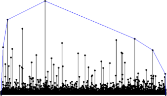
Figure 2: The least concave majorant of the Poisson point process $\rho$ on $[0,1]\times(0,\infty)$ with intensity $\alpha v^{-(\alpha+1)}\,du\,dv$, where $\alpha=2$.

this time around $(X_{1},Y_{1})$, until it hits some atom of $\rho$, denoted by $(X_{2},Y_{2})$, other than $(X_{1},Y_{1})$. Continue to rotate the line around $(X_{2},Y_{2})$, and so on. The procedure is terminated if at some time the line hits the point $(1,0)$. [As we will see later, this happens a.s. if and only if $\alpha\in(0,1)$.] Otherwise, the procedure is repeated indefinitely. Analogously, we can start with a horizontal line passing through $(X_{0},Y_{0})$ and rotate it in an anti-clockwise direction obtaining a sequence of points $(X_{-1},Y_{-1}),(X_{-2},Y_{-2}),\ldots\,$. The sequence may eventually terminate at $(0,0)$. [We will see that this happens a.s. if and only if $\alpha\in(0,1)$.] Now, join any point $(X_{k},Y_{k})$ to the next point $(X_{k+1},Y_{k+1})$ by a line segment. The polygonal path constructed in this way is the graph of the majorant $\mathfrak{C}_{\rho}$. The points $(X_{k},Y_{k})$ are called the vertices of the majorant, the intervals $[X_{k},X_{k+1}]$ are called the linearity intervals of the majorant. The least concave majorant $\mathfrak{C}_{\rho}$ is thus a piecewise linear function with at most countably many linearity intervals. We write $\mathfrak{C}_{\rho}$ in the form

$$\mathfrak{C}_{\rho}(t)=S_{k}-R_{k}t,\qquad t\in[X_{k},X_{k+1}].$$ (8)

The limiting random probability measure $\Pi_{\alpha}$ in Theorem 1.1 can be constructed as follows. For $r>0$ let $\Lambda_{r}$ be the length measure (normalized to have total mass $1$) on the circle $\{z\in\mathbb{C}\dvtx|z|=r\}$. Then

$$\Pi_{\alpha}=\sum_{k}(X_{k+1}-X_{k})\Lambda_{\exp(R_{k})},$$

where the (finite or infinite) sum is taken over all linearity intervals $[X_{k},X_{k+1}]$ of the majorant $\mathfrak{C}_{\rho}$. Thus Theorem 1.1 states that the roots of $G_{n}$ asymptotically concentrate on random circles which correspond to the linearity intervals of the majorant. The radii of these random circles are $\exp({R_{k}})$, where the $R_{k}$’s are the negatives of the slopes of the majorant. The proportion of roots on any circle is the length of the corresponding linearity interval.

Our next result describes the distribution of the complex roots of $G_{n}$ in the case $\alpha=0$. We assume that

$$\bar{F}(t):=\mathbb{P}\bigl{[}{\log}|\xi_{0}|>t\bigr{]}\qquad\mbox{is slowly varying at }{+}\infty.$$ (9)

We will show that under (9), with probability close to $1$, the complex roots of $G_{n}$ are located on just $2$ concentric circles, one of them with a radius close to $0$ and the other one with a radius close to $\infty$. A weaker result was obtained by Götze and Zaporozhets goetzezaporozhets under a more restrictive assumption on the tails. Let $\tau_{n}$ be the index of the maximal (in the sense of absolute value) coefficient of $G_{n}$, that is, $\tau_{n}\in\{0,\ldots,n\}$ is such that $|\xi_{\tau_{n}}|=\max_{k=0,\ldots,n}|\xi_{k}|$. Denote by $w_{1n},\ldots,w_{\tau_{n}n}$ the roots of the equation $\xi_{\tau_{n}}z^{\tau_{n}}+\xi_{0}=0$ and by $w_{(\tau_{n}+1)n},\ldots,w_{nn}$ the roots of the equation $\xi_{n}z^{n-\tau_{n}}+\xi_{\tau_{n}}=0$.

Theorem 1.5

Suppose that (9) is satisfied and $\xi_{0}\neq 0$ a.s. Fix some $A>0$. Then the probability that the following three statements hold simultaneously goes to $1$ as $n\to\infty$: [(3)]

$\tau_{n}$ is uniquely defined;

it is possible to renumber the roots $z_{1n},\ldots,z_{nn}$ of $G_{n}$ so that

$$|z_{kn}-w_{kn}|<e^{-n^{A}}|w_{kn}|,\qquad 1\leq k\leq n;$$

we have $|w_{kn}|<e^{-n^{A}}$ for $1\leq k\leq\tau_{n}$ and $|w_{kn}|>e^{n^{A}}$ for $\tau_{n}<k\leq n$.

Corollary 1.6

Under (9), the empirical measure $\frac{1}{n}\sum_{z\in\mathcal{Z}_{n}}\delta(z)$ converges weakly, as a random probability measure on the Riemann sphere $\bar{\mathbb{C}}$, to $U\delta(0)+(1-U)\delta(\infty)$, where $U$ is a random variable with a uniform distribution on $[0,1]$.

1.3 Properties of the majorant

In this section we study some of the properties of the least concave majorant $\mathfrak{C}_{\rho}$. Note that random convex hulls similar to $\mathfrak{C}_{\rho}$ appeared in the literature; see majumdar and the references therein. The next proposition will be used frequently.

Proposition 1.7

Let $L_{\alpha}$ be the number of linearity intervals of the majorant $\mathfrak{C}_{\rho}$. If $\alpha\in(0,1)$, then $L_{\alpha}<\infty$ a.s. If $\alpha\geq 1$, then $L_{\alpha}=\infty$ a.s. Moreover, in this case any neighborhood of $0$ (as well as any neighborhood of $1$) contains infinitely many linearity intervals of $\mathfrak{C}_{\rho}$ a.s., and we have $\lim_{k\to-\infty}R_{k}=-\infty$ and $\lim_{k\to+\infty}R_{k}=+\infty$ a.s.

Take any $\varepsilon>0$ and consider the set $D_{\varepsilon}$ of all pairs $(x,y)\in[0,1]\times(0,\infty)$ such that $y>\varepsilon x$. Integrating the intensity of $\rho$ over $D_{\varepsilon}$ we see that $\rho(D_{\varepsilon})=\infty$ a.s. if and only if $\alpha\geq 1$. If $\alpha\in(0,1)$, we have only finitely many points above any line $y>\varepsilon x$ and hence, the majorant $\mathfrak{C}_{\rho}$ has a well-defined first segment starting at $(0,0)$. On the other hand, if $\alpha\geq 1$, then no such first segment exists and consequently, we have infinitely many linearity intervals of $\rho$ in any neighborhood of $0$. By symmetry, the same is true for the point $1$. The distribution of $L_{\alpha}$ in the case $\alpha\in(0,1)$ seems difficult to characterize. In the next theorem, we compute the expectation of $L_{\alpha}$ in terms of the modular constant $C(\beta)$ introduced by Barnes barnes in his theory of the double Gamma function. Let $\psi(z)=\Gamma^{\prime}(z)/\Gamma(z)$ be the logarithmic derivative of the Gamma function. Barnes barnes showed that the following limit exists for $\beta>0$:

$$C(\beta):=\lim_{n\to\infty}\Biggl{\{}\sum_{m=1}^{n}\psi(m\beta)-\biggl{(}n+\frac{1}{2}-\frac{1}{2\beta}\biggr{)}\log(n\beta)+n\Biggr{\}}.$$ (10)

The role of the constant $C(\beta)$ in the theory of the double Gamma function is similar to the role of the Euler–Mascheroni constant $\gamma=\lim_{n\to\infty}(\sum_{k=1}^{n}\frac{1}{k}-\log n)$ in the theory of the usual Gamma function.

Theorem 1.8

For $\alpha\in(0,1)$, $\alpha\neq 1/2$, we have

$$\mathbb{E}L_{\alpha}=2+\frac{2-2\alpha}{2\alpha-1}\biggl{(}1-2C(1-\alpha)+\frac{\log(1-\alpha)-\alpha\gamma}{1-\alpha}\biggr{)}.$$ (11)

For $\alpha=1/2$ the result should be interpreted by continuity.

We will provide a representation of $\mathbb{E}L_{\alpha}$ as a definite integral in equation (73) below. Using this representation it is possible to compute the value of $\mathbb{E}L_{\alpha}$ in closed form for any rational $\alpha$. Here are some examples:

$\alpha$	$0$	$1/4$	$1/3$	$1/2$	$2/3$	$3/4$	$1$
$\mathbb{E}L_{\alpha}$	2	$(\frac{3}{2}-\frac{4}{3\sqrt{3}})\pi$	$\frac{4\pi}{3\sqrt{3}}$	$\frac{3}{2}+\frac{\pi^{2}}{8}$	$2+\frac{2\pi}{3\sqrt{3}}$	$2+\frac{\pi}{2}$	$+\infty$

The values at $\alpha=0$ and $\alpha=1$ should be understood as one-sided limits. As a corollary, we have $L_{\alpha}\to 2$ in distribution as $\alpha\downarrow 0$. Another way to see this is the following theorem.

Theorem 1.9

For $\alpha\in(0,1)$ we have $\mathbb{P}[L_{\alpha}=2]=1-\alpha$.

1.4 Real roots

Suppose now that the coefficients of the polynomial $G_{n}(z)=\sum_{k=0}^{n}\xi_{k}z^{k}$ are i.i.d. real-valued random variables. Denote by $\mathcal{R}_{n}$ the collection of real roots of $G_{n}$, and let $N_{n}=|\mathcal{R}_{n}|$ be the number of real roots. For a special family of distributions satisfying (6) with $\alpha>1$ Shepp and Farahmand sheppfarahmand showed that $\mathbb{E}N_{n}\sim\frac{2\alpha-2}{2\alpha-1}\log n$ as $n\to\infty$. In the next theorem we describe the positions of the real roots of $G_{n}$ in the limit $n\to\infty$ for every $\alpha>0$. Recall the notation $z^{\langle a\rangle}=|z|^{a}\operatorname{sgn}(z)$, where $z,a\in\mathbb{R}$. Define a point process $\Upsilon_{n}$ on $\mathbb{R}$ by

$$\Upsilon_{n}=\sum_{z\in\mathcal{R}_{n}}\delta\bigl{(}z^{\langle b_{n}\rangle}\bigr{)}.$$

Recall that a random measure $\mu$ is called a point process if the random variable $\mu(K)$ is integer-valued for every compact set $K$; see resnickbook , Section 3.1. In addition to (6) we assume that the following limit exists:

$$c:=\lim_{t\to+\infty}\frac{\mathbb{P}[\xi_{0}>t]}{\mathbb{P}[|\xi_{0}|>t]}\in[0,1].$$ (12)

Theorem 1.10

Suppose that (6) and (12) hold with some $\alpha>0$. Write $p=\mathbb{P}[\xi_{0}>0]$ and suppose that $\xi_{0}\neq 0$ a.s. [(2)]

For $\alpha\geq 1$ the point process $\Upsilon_{n}$ converges weakly to some point process $\Upsilon_{\alpha,c}$ on $\mathbb{R}\setminus\{0\}$.

For $\alpha\in(0,1)$ the point process $\Upsilon_{2n}$ (resp., $\Upsilon_{2n+1}$) converges weakly to some point process $\Upsilon_{\alpha,c,p}^{+}$ (resp., $\Upsilon_{\alpha,c,p}^{-}$) on $[-\infty,+\infty]$ and on $\mathbb{R}$.

The somewhat technical description of the point processes $\Upsilon_{\alpha,c}$, $\Upsilon_{\alpha,c,p}^{\pm}$ is postponed to Section 6.1. Recall that by Theorem 1.1 the complex roots of $G_{n}$ are located asymptotically on a set of random circles. Each circle crosses the real line at $2$ points. We will show that any of these points may or may not be a real root of $G_{n}$ with some probabilities. For $\alpha\in(0,1)$ the point processes $\Upsilon_{\alpha,c,p}^{\pm}$ have a.s. finitely many atoms, whereas for $\alpha\geq 1$ the atoms of the point process $\Upsilon_{\alpha,c}$ accumulate a.s. at $\pm 0$ and $\pm\infty$. (Of course, this is related to Proposition 1.7.) Since the map assigning to a finite counting measure on $[-\infty,\infty]$ its total mass is continuous (locally constant) in the weak topology, we obtain the following statement on the number of real roots of $G_{n}$.

Corollary 1.11

Suppose that (6) and (12) hold with $\alpha\in(0,1)$ and let $\xi_{0}\neq 0$ a.s. Then the sequence $\{N_{2n}\}_{n\in\mathbb{N}}$ (resp., $\{N_{2n+1}\}_{n\in\mathbb{N}}$) converges in distribution to a random variable $N^{+}_{\alpha,c,p}$ (resp., $N^{-}_{\alpha,c,p}$).

Remark 1.12.

The expectations $\mathbb{E}N^{+}_{\alpha,c,p}$ and $\mathbb{E}N^{-}_{\alpha,c,p}$ can be computed using the representation of the point processes $\Upsilon_{\alpha,c,p}^{\pm}$ given in Section 6.1.

$$\mathbb{E}N^{+}_{\alpha,c,p}=\mathbb{E}N^{-}_{\alpha,c,p}=\bigl{(}2c(1-c)+\tfrac 12\bigr{)}(\mathbb{E}L_{\alpha}-2)+2(p+c-2pc)+1.$$

For instance, if the distribution of $\xi_{0}$ is symmetric with respect to the origin, then both expectation are equal to $\mathbb{E}L_{\alpha}$. We conjecture that the convergence in Corollary 1.11 holds in the $L^{1}$-sense.

Remark 1.13.

The behavior of $N_{n}$ in the case $\alpha=1$ remains open. For $\alpha=1$ the result of sheppfarahmand turns formally into $\mathbb{E}N_{n}=o(\log n)$, whereas the fact that $\Upsilon_{1,c}$ has infinitely many atoms a.s. suggests that $\mathbb{E}N_{n}$ should be infinite. It is natural to conjecture that for $\alpha=1$, we should have $\mathbb{E}N_{n}\sim K\log\log n$ for some $K>0$.

Finally, we investigate the number of real roots of $G_{n}$ in the case $\alpha=0$.

Theorem 1.14

Suppose that (9) and (12) hold, $\xi_{0}\neq 0$ a.s., and write $p=\mathbb{P}[\xi_{0}>0]$. Then, the sequence $\{N_{2n}\}_{n\in\mathbb{N}}$ converges weakly to a random variable $N^{+}_{0,c,p}$ and the sequence $\{N_{2n+1}\}_{n\in\mathbb{N}}$ converges weakly to a random variable $N^{-}_{0,c,p}$ such that

$$\mathbb{P}\bigl{[}N^{+}_{0,c,p}=m\bigr{]} = \cases{\frac{1}{2}\bigl{(}cp^{2}+(1-c)(1-p)^{2}\bigr{)},&\quad$m=0$,\vspace*{2pt}\cr\frac{1}{2}+p(1-p),&\quad$m=2$,\vspace*{2pt}\cr\frac{1}{2}\bigl{(}c(1-p)^{2}+(1-c)p^{2}\bigr{)},&\quad$m=4$;}$$ (13)

$$\mathbb{P}\bigl{[}N^{-}_{0,c,p}=m\bigr{]} = \cases{1-p-c+2pc,&\quad$m=1$,\cr p+c-2pc,&\quad$m=3$.}$$ (14)

Remark 1.15.

If the distribution of $\xi_{0}$ is symmetric with respect to the origin, we obtain the following results: $N^{+}_{0,1/2,1/2}$ takes the values $0,2,4$ with probabilities $1/8,3/4,1/8$, and $N^{-}_{0,1/2,1/2}$ takes the values $1,3$ with probabilities $1/2,1/2$.

Remark 1.16.

For fixed $p\in[0,1]$, both

$$\min_{c\in[0,1]}\mathbb{E}N^{+}_{0,c,p}\quad\mbox{and}\quad\min_{c\in[0,1]}\mathbb{E}N^{-}_{0,c,p}$$

are equal to $1+2\min(p,1-p)$. The same number appeared in zn as the minimal expected number of real roots of a random polynomial.

1.5 Emergence of the majorant

The least concave majorant which we encountered above is reminiscent of the Newton polygons appearing when solving polynomial equations with non-Archimedian (e.g., $p$-adic) coefficients; see koblitzbook , Chapter IV. Of course, our random polynomial $G_{n}$ has complex (Archimedian) coefficients. However, non-Archimedian effects will appear in the following way. Consider the sum $c_{1}e^{nx_{1}}+\cdots+c_{d}e^{nx_{d}}$, where $x_{i}>0$ and $c_{i}\in\mathbb{C}$. If $n$ is large, then the most easy way such sum may become zero is if two terms, say $c_{k}e^{nx_{k}}$ and $c_{l}e^{nx_{l}}$, cancel each other and the other terms are much smaller than these two. We will show that under (6) similar considerations apply to the polynomial $G_{n}(z)=\sum_{j=0}^{n}\xi_{j}z^{j}$ with high probability: $z\in\mathbb{C}$ is a root of $G_{n}$ essentially only if two of the terms, $\xi_{k}z^{k}$ and $\xi_{l}z^{l}$, cancel each other, and all other terms are of smaller order. Geometrically, this means that the points $(k,{\log}|\xi_{k}|)$ and $(l,{\log}|\xi_{l}|)$ are neighboring vertices of the least concave majorant of the set $\{(j,{\log}|\xi_{j}|)\dvtx j=0,\ldots,n\}$. The nonzero roots of $\xi_{k}z^{k}+\xi_{l}z^{l}=0$ form a regular polygon inscribed into the circle whose radius is the exponential of minus the slope of the line joining the points $(k,{\log}|\xi_{k}|)$ and $(l,{\log}|\xi_{l}|)$. Taking the union of such circles over all segments of the majorant we obtain essentially all the roots of $G_{n}$. To complete the argument, we need to find the limiting form of the majorant as $n\to\infty$. This is done using the following proposition which is known in the extreme-value theory; see resnickbook , Corollary 4.19(ii).

Proposition 1.17

Let $\xi_{0},\xi_{1},\ldots$ be i.i.d. random variables satisfying (6). Then the following convergence holds weakly on the space of locally finite counting measures on $[0,1]\times(0,\infty]$:

$$\rho_{n}:=\sum_{k=0}^{n}\delta\biggl{(}\frac{k}{n},\frac{{\log}|\xi_{k}|}{a_{n}}\biggr{)}\mathop{\longrightarrow}_{n\to\infty}^{w}\sum_{i=1}^{\infty}\delta(U_{i},V_{i})=:\rho.$$

Here, $\rho$ is a Poisson point process on $[0,1]\times(0,\infty)$ with intensity $\alpha v^{-(\alpha+1)}\,du\,dv$. We agree that the points for which ${\log}|\xi_{k}|\leq 0$ are not counted in $\rho_{n}$.

The paper of Shepp and Farahmand sheppfarahmand seems to be the only work where random polynomials with coefficients satisfying (6) have been considered. The method used there (characteristic functions) is very different from our approach based on majorants. Whether the results of sheppfarahmand can be recovered (or strengthened) using our approach remains open. Let us also mention that the least concave majorant appeared in the theory of entire functions; see valironbook , page 28. For example, Hardy hardy showed that the zeros of the deterministic entire function $\sum_{k=0}^{\infty}z^{k^{3}}/(k^{3})!$ have a circle structure similar to the structure of zeros of $G_{n}$ under (6). Eigenvalues of random matrices with i.i.d. heavy-tailed entries have been studied in bordenaveetal .

2 The main lemma

The next lemma is the key step in the proof. Let $g(z)=\sum_{j=0}^{n}a_{j}z^{j}$ be a (deterministic) polynomial with complex coefficients. Suppose that the points $(k,{\log}|a_{k}|)$ and $(l,{\log}|a_{l}|)$, where $0\leq k<l\leq n$, are neighboring vertices on the least concave majorant of the set $\{(j,{\log}|a_{j}|)\dvtx j=0,\ldots,n\}$. That is to say, for some $s,r\in\mathbb{R}$, we have

$${\log}|a_{k}| = s-kr,\qquad{\log}|a_{l}|=s-lr,$$

$$h:\! = \mathop{\min_{0\leq j\leq n}}_{j\neq k,l}\bigl{(}s-jr-{\log}|a_{j}|\bigr{)}>0.$$

Here, we have assumed that no three points of the majorant are on the same line. Note that $h$ measures the gap between the line passing through the points $(k,{\log}|a_{k}|)$, $(l,{\log}|a_{l}|)$ and the points lying below this line.

Lemma 2.1

If $\delta>0$ is such that $ne^{\delta n-h}<1-e^{-\delta}$, then in the ring $e^{r-\delta}<|z|<e^{r+\delta}$ there are exactly $l-k$ roots of $g$. Moreover, if $\zeta$ is such that $2ne^{2\delta n-h}<\zeta<\frac{\pi}{l-k}$, then the set

$$\biggl{\{}z\in\mathbb{C}\dvtx e^{r-\delta}<|z|<e^{r+\delta},\biggl{|}\arg z-\frac{\varphi+2\pi m}{l-k}\biggr{|}\leq\zeta\biggr{\}},$$ (16)

where $\varphi=\arg(-a_{k}/a_{l})$, contains exactly one root of $g$ for every $m=1,\ldots,\break l-k$.

Here, we agree to understand the distance between the arguments of complex numbers as the geodesic distance on the unit circle. Also, let the index $j$ be always restricted to $0\leq j\leq n$.

Proof of Lemma 2.1 We will prove a stronger version of the lemma. Namely, we will show that the statement holds for the family of polynomials

$$g_{t}(z)=a_{k}z^{k}+a_{l}z^{l}+t\sum_{j\neq k,l}a_{j}z^{j},\qquad 0\leq t\leq 1.$$

Note that in particular, $g_{0}(z)=a_{k}z^{k}+a_{l}z^{l}$ and $g_{1}(z)=g(z)$. Let $z\in\mathbb{C}$ be such that $|z|=e^{r-\delta}$. It follows from (2) that

$$t\biggl{|}\sum_{j\neq k,l}a_{j}z^{j}\biggr{|}\leq\sum_{j\neq k,l}e^{s-jr-h}e^{j(r-\delta)}<ne^{s-h}.$$

On the other hand, again by (2),

$$\bigl{|}a_{k}z^{k}+a_{l}z^{l}\bigr{|}\geq\bigl{|}a_{k}z^{k}\bigr{|}-\bigl{|}a_{l}z^{l}\bigr{|}=e^{s}e^{-\delta k}\bigl{(}1-e^{-\delta(l-k)}\bigr{)}>e^{s-\delta n}\bigl{(}1-e^{-\delta}\bigr{)}.$$

Since $ne^{\delta n-h}<1-e^{-\delta}$ holds, everywhere on the circle $|z|=e^{r-\delta}$ we have

$$\bigl{|}a_{k}z^{k}+a_{l}z^{l}\bigr{|}>t\biggl{|}\sum_{j\neq k,l}a_{j}z^{j}\biggr{|}.$$ (17)

Hence, by Rouché’s theorem, the polynomial $g_{t}$ has exactly $k$ roots in the circle $|z|\leq e^{r-\delta}$.

Let now $z\in\mathbb{C}$ be such that $|z|=e^{r+\delta}$. Then

$$t\biggl{|}\sum_{j\neq k,l}a_{j}z^{j}\biggr{|}\leq\sum_{j\neq k,l}e^{s-jr-h}e^{j(r+\delta)}<ne^{s-h+\delta n}.$$ (18)

On the other hand,

$$\bigl{|}a_{k}z^{k}+a_{l}z^{l}\bigr{|}\geq\bigl{|}a_{l}z^{l}\bigr{|}-\bigl{|}a_{k}z^{k}\bigr{|}=e^{s}e^{\delta l}\bigl{(}1-e^{\delta(k-l)}\bigr{)}>e^{s}\bigl{(}1-e^{-\delta}\bigr{)}.$$

Therefore, inequality (17) also holds everywhere on the circle $|z|=e^{r+\delta}$. It follows from Rouché’s theorem that the polynomial $g_{t}$ has exactly $l$ roots in the circle $|z|\leq e^{r+\delta}$. Hence, the polynomial $g_{t}$ has exactly $l-k$ roots in the ring $e^{r-\delta}\leq|z|\leq e^{r+\delta}$.

Let us now show that these $l-k$ roots are located approximately at the same positions as the nonzero roots of the equation $a_{l}z^{l}+a_{k}z^{k}=0$. Let $z_{0}$ be some root of $g_{t}$ satisfying $e^{r-\delta}\leq|z_{0}|\leq e^{r+\delta}$. Then, repeating the argument of (18), we obtain that

$$\bigl{|}a_{l}z_{0}^{l}+a_{k}z_{0}^{k}\bigr{|}=\biggl{|}\sum_{j\neq k,l}a_{j}z_{0}^{j}\biggr{|}<ne^{s-h+\delta n}.$$ (19)

Recall that $\varphi=\arg(-a_{k}/a_{l})$. The arguments of the nonzero roots of the equation $a_{l}z^{l}+a_{k}z^{k}=0$ are given by $\frac{\varphi+2\pi m}{l-k}$, where $m=1,\ldots,l-k$, and their moduli are equal to $e^{r}$. Let

$$\varsigma=\min_{m=1,\ldots,l-k}\biggl{|}\arg z_{0}-\frac{\varphi+2\pi m}{l-k}\biggr{|}.$$

Note that $\varsigma\in[0,\frac{\pi}{l-k}]$ by definition. Then

$$\bigl{|}\arg\bigl{(}a_{l}z_{0}^{l}\bigr{)}-\arg\bigl{(}-a_{k}z_{0}^{k}\bigr{)}\bigr{|}=\bigl{|}\arg z_{0}^{l-k}-\varphi\bigr{|}=(l-k)\varsigma.$$

By the inequality $|z_{1}-z_{2}|\geq 2|z_{1}|\sin(|{\arg z_{1}}-\arg z_{2}|/2)$ valid for $|z_{1}|\leq|z_{2}|$ and the inequality $\sin x\geq\frac{2}{\pi}x$ valid for $x\in[0,\frac{\pi}{2}]$, we obtain

$$\bigl{|}a_{l}z_{0}^{l}+a_{k}z_{0}^{k}\bigr{|}\geq 2e^{s-\delta l}\sin\biggl{(}\frac{(l-k)\varsigma}{2}\biggr{)}\geq\frac{1}{2}e^{s-\delta n}\varsigma.$$ (20)

It follows from (19) and (20) that $\varsigma<2ne^{2\delta n-h}$ and hence $\varsigma<\zeta$. Therefore, every root $z_{0}$ of $g_{t}$ such that $e^{r-\delta}\leq|z_{0}|\leq e^{r+\delta}$ is contained in a set of the form (16) for some $m=1,\ldots,l-k$. To complete the proof, it remains to show that every set (16) contains exactly one root of $g_{t}$. Since $\zeta<\frac{\pi}{l-k}$, all these sets are disjoint. By the above, $g_{t}$ does not vanish on their boundaries. It follows from this and the argument principle that the number of roots of $g_{t}$ in any set (16) is continuous as a function of $t\in[0,1]$ and hence, constant. Obviously, every set (16) contains exactly one root of $g_{0}$ and hence, exactly one root of $g_{t}$.

3 Least concave majorants and weak convergence

Proposition 1.17states the convergence of the point process $\rho_{n}$ formed by the logarithms of the coefficients of the random polynomial $G_{n}$ to the limiting Poisson process $\rho$. We will need to deduce from this the weak convergence of certain functionals of $\rho_{n}$ to the same functionals of $\rho$. This will be done using the following well-known continuous mapping theorem; see resnickbook , page 152, or billingsleybook , page 30.

Proposition 3.1

Let $F\dvtx M_{1}\to M_{2}$ be a map between two metric spaces $(M_{1},d_{1})$ and $(M_{2},d_{2})$. Let $X_{n}$ be a sequence of $M_{1}$-valued random variables converging weakly to some $M_{1}$-valued random variable $X$. If $F$ satisfies

$$\mathbb{P}[F\mbox{ is discontinuous at }X]=0,$$

then $F(X_{n})$ converges weakly to $F(X)$ on $(M_{2},d_{2})$.

In order to apply Proposition 3.1 we need to prove the a.s. continuity of the functionals under consideration. This is the aim of the present section. First we introduce some notation. Let $\mathfrak{M}$ be the set of locally finite counting measures $\mu$ on $[0,1]\times(0,\infty]$ such that $\mu([0,1]\times\{\infty\})=0$. We endow $\mathfrak{M}$ with the topology of vague convergence. Every $\mu\in\mathfrak{M}$ can be written in the form $\mu=\sum_{i}\delta(u_{i},v_{i})$, where $i$ ranges in some at most countable index set and $u_{i}\in[0,1]$, $v_{i}\in(0,\infty)$. The number of atoms of $\mu$ in a set of the form $[0,1]\times[\varepsilon,\infty)$ is finite for every $\varepsilon>0$, but the atoms of $\mu$ may (and often will) have accumulation points in the set $[0,1]\times\{0\}$.

The least concave majorant of $\mu\in\mathfrak{M}$ is a function $\mathfrak{C}_{\mu}\dvtx[0,1]\to[0,\infty)$ defined by $\mathfrak{C}_{\mu}(t)=\inf_{f}f(t)$, where the infimum is taken over all concave functions $f\dvtx[0,1]\to[0,\infty)$ such that $f(u_{i})\geq v_{i}$ for all $i$. We write the piecewise linear function $\mathfrak{C}_{\mu}$ in the form

$$\mathfrak{C}_{\mu}(t)=s_{k}-r_{k}t,\qquad t\in[x_{k},x_{k+1}],$$ (21)

where $k$ ranges over a finite or infinite discrete subinterval of $\mathbb{Z}$. We set $y_{k}=\mathfrak{C}_{\mu}(x_{k})$. The intervals $[x_{k},x_{k+1}]$ (called the linearity intervals of the majorant) are always supposed to be chosen in such a way that the points $(x_{k},y_{k})$ and $(x_{k+1},y_{k+1})$ are atoms of $\mu$, and there are no further atoms of $\mu$ on the segment joining these two points. Fix some small $\kappa\in(0,1/2)$. Given a counting measure $\mu\in\mathfrak{M}$, we define the indices $q^{\prime}=q^{\prime}_{\kappa}(\mu)$ and $q^{\prime\prime}=q^{\prime\prime}_{\kappa}(\mu)$ by the conditions $x_{q^{\prime}}\leq\kappa<x_{q^{\prime}+1}$ and $x_{q^{\prime\prime}-1}<1-\kappa\leq x_{q^{\prime\prime}}$.

Let $\mathfrak{M}_{1}$ be the set of all counting measures $\mu\in\mathfrak{M}$ with the following properties: [(3)]

both $0$ and $1$ are accumulation points for the linearity intervals of $\mathfrak{C}_{\mu}$;

$\mu(L)\leq 2$ for every line $L\subset\mathbb{R}^{2}$;

no atom of $\mu$ has first coordinate $\kappa$ or $1-\kappa$. Note that every $\mu\in\mathfrak{M}_{1}$ has only simple atoms. Denote by $\mathfrak{N}$ the space of finite measures on $\mathbb{R}$ endowed with the weak topology. Let $V_{k}(\mu)$ be the subset of $[0,1]\times[0,\infty)$ consisting of $[0,1]\times\{0\}$ together with all atoms of $\mu$, except for $(x_{k},y_{k})$ and $(x_{k+1},y_{k+1})$.

Lemma 3.2

The following mappings are continuous on $\mathfrak{M}_{1}$: [(3)]

$\Psi_{1}\dvtx\mathfrak{M}\to\mathfrak{N}$ defined by $\Psi_{1}(\mu)=\sum_{k=q^{\prime}}^{q^{\prime\prime}-1}(x_{k+1}-x_{k})\delta(r_{k})$;

$H_{1}\dvtx\mathfrak{M}\to\mathbb{R}$ defined by $H_{1}(\mu)=\min\{s_{k}-r_{k}u-v\}$, where the minimum is over $q^{\prime}\leq k<q^{\prime\prime}$ and $(u,v)\in V_{k}(\mu)$;

$L_{1}\dvtx\mathfrak{M}\to\mathbb{R}$ defined by $L_{1}(\mu)=\min_{q^{\prime}\leq k<q^{\prime\prime}}(x_{k+1}-x_{k})$.

Let $\{\mu_{n}\}_{n\in\mathbb{N}}\subset\mathfrak{M}$ be a sequence converging to $\mu\in\mathfrak{M}_{1}$ in the vague topology on $[0,1]\times(0,\infty]$. Let $\varepsilon>0$ be such that $2\varepsilon<\min_{q^{\prime}\leq k<q^{\prime\prime}}\{s_{k},\break s_{k}-r_{k}\}$. Note that the minimum is strictly positive by the definition of $\mathfrak{M}_{1}$. Denote by $(u_{l},v_{l})$, where $1\leq l\leq m$, all atoms of $\mu$ (excluding those which are vertices of $\mathfrak{C}_{\mu}$) with the property that $v_{l}>\varepsilon$. Since $\mu_{n}\to\mu$ vaguely, we can find (see resnickbook , Proposition 3.13) atoms of $\mu_{n}$ denoted by $(x_{kn},y_{kn})$ (where $q^{\prime}\leq k\leq q^{\prime\prime}$) and $(u_{ln},v_{ln})$ (where $1\leq l\leq m$) such that

$$\lim_{n\to\infty}(x_{kn},y_{kn}) = (x_{k},y_{k}),\qquad q^{\prime}\leq k\leq q^{\prime\prime},$$ (22)

$$\lim_{n\to\infty}(u_{ln},v_{ln}) = (u_{l},v_{l}),\qquad 1\leq l\leq m.$$ (23)

Moreover, since the vague convergence was required to hold on $[0,1]\times(0,\infty]$, there are no other atoms of $\mu_{n}$ having a second coordinate exceeding $2\varepsilon$, provided that $n$ is sufficiently large. It follows that as $n\to\infty$ and for all $q^{\prime}\leq k<q^{\prime\prime}$,

$$r_{kn}:=-\frac{y_{(k+1)n}-y_{kn}}{x_{(k+1)n}-x_{kn}}\to r_{k},\qquad s_{kn}:=y_{kn}+r_{kn}x_{kn}\to s_{k}.$$ (24)

In particular, for sufficiently large $n$, all $q^{\prime}\leq k<q^{\prime\prime}$ and all $1\leq l\leq m$,

$$s_{kn}-r_{kn}u_{ln}>v_{ln},\qquad\inf_{u\in[0,1]}(s_{kn}-r_{kn}u)>2\varepsilon.$$

It follows that for sufficiently large $n$, the segment joining the points $(x_{kn},y_{kn})$ and $(x_{(k+1)n},y_{(k+1)n})$ belongs to the majorant of $\mu_{n}$ for every $q^{\prime}\leq k<q^{\prime\prime}$. Also, $x_{q^{\prime}n}<\kappa<x_{(q^{\prime}+1)n}$ and $x_{(q^{\prime\prime}-1)n}<1-\kappa<x_{q^{\prime\prime}n}$.

By using (22), (23), (24) and letting $\varepsilon\downarrow 0$, we obtain that $H_{1}(\mu_{n})\to H_{1}(\mu)$ and $L_{1}(\mu_{n})\to L_{1}(\mu)$ as $n\to\infty$. This proves the continuity of $H_{1}$ and $L_{1}$ on $\mathfrak{M}_{1}$. To prove the continuity of $\Psi_{1}$, note that for every continuous, bounded function $f\dvtx\mathbb{R}\to\mathbb{R}$,

$$\int_{\mathbb{R}}f\,d\Psi_{1}(\mu_{n})=\sum_{k=q^{\prime}}^{q^{\prime\prime}-1}(x_{(k+1)n}-x_{kn})f(r_{kn})\mathop{\longrightarrow}_{n\to\infty}\sum_{k=q^{\prime}}^{q^{\prime\prime}-1}(x_{k+1}-x_{k})f(r_{k}).$$

Thus, $\Psi_{1}(\mu_{n})\to\Psi_{1}(\mu)$ weakly, which proves the continuity of $\Psi_{1}$.

The next lemma will be needed to prove our main results for $\alpha\in(0,1)$. Let $\mathfrak{M}_{0}$ be the set of all nonzero counting measures $\mu\in\mathfrak{M}$ with the following properties: [(3)]

the number of linearity intervals of $\mathfrak{C}_{\mu}$ is finite and $\mathfrak{C}_{\mu}(0)=\mathfrak{C}_{\mu}(1)=0$;

$\bar{\mu}(L)\leq 2$ for every line $L\subset\mathbb{R}^{2}$, where $\bar{\mu}=\mu+\delta(0,0)+\delta(1,0)$;

no atom of $\mu$ has first coordinate $\kappa$ or $1-\kappa$.

Lemma 3.3

The following mappings are continuous on $\mathfrak{M}_{0}$: [(3)]

$\Psi_{0}\dvtx\mathfrak{M}\to\mathfrak{N}$ defined by $\Psi_{0}(\mu)=\sum_{k}(x_{k+1}-x_{k})\delta(r_{k})$, where the sum is over all linearity intervals $[x_{k},x_{k+1}]$ of the majorant $\mathfrak{C}_{\mu}$;

$H_{0}\dvtx\mathfrak{M}\to[0,\infty]$ defined by $H_{0}(\mu)=\min\{s_{k}-r_{k}u-v\}$, where the minimum is over $q^{\prime}<k<q^{\prime\prime}-1$ and $(u,v)\in V_{k}(\mu)$;

$L_{0}\dvtx\mathfrak{M}\to[0,\infty]$ defined by $L_{0}(\mu)=\min_{q^{\prime}<k<q^{\prime\prime}-1}(x_{k+1}-x_{k})$.

Remark 3.4.

In fact, $\Psi_{0}$ is continuous on the whole of $\mathfrak{M}$, but we will not need this. The minimum over an empty set is $+\infty$.

Proof of Lemma 3.3 Let $\{\mu_{n}\}_{n\in\mathbb{N}}\subset\mathfrak{M}$ be a sequence converging vaguely to $\mu\in\mathfrak{M}_{0}$. The majorant $\mathfrak{C}_{\mu}$ is a piecewise linear function whose graph is a broken line connecting the points denoted by $(x_{k},y_{k})$, where $p^{\prime}\leq k\leq p^{\prime\prime}$ and $(x_{p^{\prime}},y_{p^{\prime}})=(0,0)$, $(x_{p^{\prime\prime}},y_{p^{\prime\prime}})=(1,0)$. For $p^{\prime}<k<p^{\prime\prime}$, the point $(x_{k},y_{k})$ is an atom of $\mu$. Denote by $(u_{l},v_{l})$, where $1\leq l\leq m$, all atoms of $\mu$ (excluding those which are vertices of the majorant) with the property that $v_{l}>\varepsilon$, where $\varepsilon>0$ is a number such that $2\varepsilon<\min_{p^{\prime}<k<p^{\prime\prime}-1}\{s_{k},s_{k}-r_{k}\}$. Note that the minimum is taken over the set of linearity intervals of the majorant excluding the first and the last interval. If the majorant consists of just two segments, then the minimum is $+\infty$. The vague convergence $\mu_{n}\to\mu$ implies (see resnickbook , Proposition 3.13) that we can find atoms of $\mu_{n}$ denoted by $(x_{kn},y_{kn})$ (where $p^{\prime}<k<p^{\prime\prime}$) and $(u_{ln},v_{ln})$ (where $1\leq l\leq m$) such that

$$\lim_{n\to\infty}(x_{kn},y_{kn}) = (x_{k},y_{k}),\qquad p^{\prime}<k<p^{\prime\prime},$$ (25)

$$\lim_{n\to\infty}(u_{ln},v_{ln}) = (u_{l},v_{l}),\qquad 1\leq l\leq m.$$ (26)

Moreover, if $n$ is sufficiently large, then there are no other atoms of $\mu_{n}$ having a second coordinate exceeding $2\varepsilon$. It follows that as $n\to\infty$ and for all $p^{\prime}<k<p^{\prime\prime}-1$,

$$r_{kn}:=-\frac{y_{(k+1)n}-y_{kn}}{x_{(k+1)n}-x_{kn}}\to r_{k},\qquad s_{kn}:=y_{kn}+r_{kn}x_{kn}\to s_{k}.$$ (27)

Note that by concavity $s_{k}-r_{k}u_{l}>v_{l}$ for all $p^{\prime}<k<p^{\prime\prime}-1$ and $1\leq l\leq m$. Thus, for sufficiently large $n$,

$$s_{kn}-r_{kn}u_{ln}>v_{ln},\qquad\inf_{u\in[0,1]}(s_{kn}-r_{kn}u)>2\varepsilon.$$

This means that for sufficiently large $n$ the segment joining the points $(x_{kn},y_{kn})$ and $(x_{(k+1)n},y_{(k+1)n})$ belongs to the majorant of $\mu_{n}$ for every $p^{\prime}<k<p^{\prime\prime}-1$. Also, $x_{q^{\prime}n}<\kappa<x_{(q^{\prime}+1)n}$ and $x_{(q^{\prime\prime}-1)n}<1-\kappa<x_{q^{\prime\prime}n}$.

From (25), (26), (27) we obtain that $H_{0}(\mu_{n})\to H_{0}(\mu)$ and $L_{0}(\mu_{n})\to L_{0}(\mu)$ as $n\to\infty$. This proves the continuity of $H_{0}$ and $L_{0}$ on $\mathfrak{M}_{0}$. To prove the continuity of $\Psi_{0}$ we need to show that for every continuous, bounded function $f\dvtx\mathbb{R}\to[0,\infty)$,

$$\lim_{n\to\infty}\int_{\mathbb{R}}f\,d\Psi_{0}(\mu_{n})=\int_{\mathbb{R}}f\,d\Psi_{0}(\mu).$$ (28)

By (25) and (27), we have

$$\quad\lim_{n\to\infty}\sum_{p^{\prime}<k<p^{\prime\prime}-1}(x_{(k+1)n}-x_{kn})f(r_{kn})=\sum_{p^{\prime}<k<p^{\prime\prime}-1}(x_{k+1}-x_{k})f(r_{k}).$$ (29)

However, we have to be more careful about approximating the first and the last segments of $\mathfrak{C}_{\mu}$. Denote by $(x_{kn},y_{kn})$, where $k\leq p^{\prime}+1$, the vertices of the majorant of $\mu_{n}$ (counted from left to right) with the property $x_{kn}\leq x_{(p^{\prime}+1)n}$. Note that the number of such vertices is, in general, arbitrary and may be infinite. Since the first segment of the majorant of $\mu$ joins $(0,0)$ and $(x_{p^{\prime}+1},y_{p^{\prime}+1})$, all points $(u_{ln},v_{ln})$, where $1\leq l\leq m$, are located below the line joining $(0,0)$ and $(x_{(p^{\prime}+1)n},y_{(p^{\prime}+1)n})$ for large $n$. Therefore, for large $n$ there are no atoms of $\mu_{n}$ above the line joining $(0,2\varepsilon)$ and $(x_{(p^{\prime}+1)n},y_{(p^{\prime}+1)n})$. Hence,

$$r_{p^{\prime}n}:\! = -\frac{y_{(p^{\prime}+1)n}-y_{p^{\prime}n}}{x_{(p^{\prime}+1)n}-x_{p^{\prime}n}}$$

$$\in \biggl{[}-\frac{y_{(p^{\prime}+1)n}-2\varepsilon}{x_{(p^{\prime}+1)n}},-\frac{y_{(p^{\prime}+1)n}}{x_{(p^{\prime}+1)n}}\biggr{]},\qquad x_{p^{\prime}n}<2\varepsilon\frac{y_{(p^{\prime}+1)n}}{x_{(p^{\prime}+1)n}}.$$

It follows that $r_{p^{\prime}n}\to r_{p^{\prime}}$ as $n\to\infty$. The contribution of linearity intervals to the left of $x_{p^{\prime}n}$ can be estimated as follows: for large $n$,

$$\sum_{k<p^{\prime}}(x_{(k+1)n}-x_{kn})f(r_{kn})\leq x_{p^{\prime}n}\|f\|_{\infty}\leq 4\varepsilon\frac{y_{p^{\prime}+1}}{x_{p^{\prime}+1}}\|f\|_{\infty}.$$

Since $\varepsilon>0$ can be made as small as we like, we have

$$\lim_{n\to\infty}\sum_{k\leq p^{\prime}}(x_{(k+1)n}-x_{kn})f(r_{kn})=x_{p^{\prime}+1}f(r_{p^{\prime}}).$$ (30)

Similar arguments can be applied to the part of the majorant of $\mu_{n}$ located to the right of $(x_{(p^{\prime\prime}-1)n},y_{(p^{\prime\prime}-1)n})$: with straightforward notation,

$$\lim_{n\to\infty}\sum_{k\geq p^{\prime\prime}-1}(x_{(k+1)n}-x_{kn})f(r_{kn})=(1-x_{p^{\prime\prime}-1})f(r_{p^{\prime\prime}-1}).$$ (31)

Bringing (29), (30), (31) together we obtain (28).

In our proofs we will often consider some “good” random event $E_{n}(\kappa)$ under which we will be able to localize the roots of $G_{n}$. The next lemma will be useful.

Lemma 3.5

Let $\{S_{n}\}_{n\in\mathbb{N}}$ and $S$ be random variables defined on a common probability space. Suppose that for each $\kappa>0$ we have random events $\{E_{n}(\kappa)\}_{n\in\mathbb{N}}$ and random variables $\{S_{n}(\kappa)\}_{n\in\mathbb{N}}$, $S(\kappa)$ such that the following conditions hold: [(4)]

for every $\kappa>0$, $S_{n}(\kappa)\to S(\kappa)$ in distribution as $n\to\infty$;

$S(\kappa)\to S$ in distribution as $\kappa\downarrow 0$;

$\lim_{\kappa\downarrow 0}\liminf_{n\to\infty}\mathbb{P}[E_{n}(\kappa)]=1$;

$|S_{n}(\kappa)-S_{n}|<m_{n}(\kappa)$ on $E_{n}(\kappa)$, where $\lim_{\kappa\downarrow 0}\limsup_{n\to\infty}m_{n}(\kappa)=0$. Then, $S_{n}\to S$ in distribution as $n\to\infty$.

Let $f\dvtx\mathbb{R}\to\mathbb{R}$ be a continuous function with compact support. Write $C=\|f\|_{\infty}$. Take some $\varepsilon>0$. We can choose $\kappa=\kappa(\varepsilon)>0$ such that

$$\bigl{|}\mathbb{E}f\bigl{(}S(\kappa)\bigr{)}-\mathbb{E}f(S)\bigr{|} < \varepsilon,\qquad\limsup_{n\to\infty}\mathbb{P}\bigl{[}E_{n}^{c}(\kappa)\bigr{]}<\varepsilon,$$

$$\limsup_{n\to\infty}m_{n}(\kappa) < \varepsilon.$$

Here, $E_{n}^{c}(\kappa)$ denotes the complement of $E_{n}(\kappa)$. After having fixed $\kappa$ we choose $n_{0}=n_{0}(\varepsilon)$ such that for all $n>n_{0}$,

$$\quad\bigl{|}\mathbb{E}f\bigl{(}S_{n}(\kappa)\bigr{)}-\mathbb{E}f\bigl{(}S(\kappa)\bigr{)}\bigr{|}<\varepsilon,\qquad\mathbb{P}\bigl{[}E_{n}^{c}(\kappa)\bigr{]}<2\varepsilon,\qquad m_{n}(\kappa)<2\varepsilon.$$ (33)

Denoting by $\omega_{f}(\delta)=\sup_{|z_{1}-z_{2}|\leq\delta}|f(z_{1})-f(z_{2})|$ the continuity modulus of $f$, we have

$$\quad\bigl{|}\mathbb{E}f(S_{n})-\mathbb{E}f\bigl{(}S_{n}(\kappa)\bigr{)}\bigr{|}\leq\omega_{f}\bigl{(}m_{n}(\kappa)\bigr{)}+2C\mathbb{P}\bigl{[}E_{n}^{c}(\kappa)\bigr{]}\leq\omega_{f}(2\varepsilon)+4C\varepsilon.$$ (34)

Taking $\varepsilon\downarrow 0$ in (3), (33), (34), we obtain $\lim_{n\to\infty}\mathbb{E}f(S_{n})=\mathbb{E}f(S)$.

4 Proof of Theorem 1.1

4.1 Notation

Let $\xi_{0},\xi_{1},\ldots$ be i.i.d. random variables satisfying (6). Consider the least concave majorant $\mathfrak{C}_{n}$ of the set $\{(k,{\log}|\xi_{k}|)\dvtx k=0,\ldots,n\}$, where we agree to exclude points with ${\log}|\xi_{k}|\leq 0$ from consideration. By definition, $\mathfrak{C}_{n}(t)=\inf_{f}f(t)$ for all $t\in[0,n]$, where the infimum is taken over all concave functions $f\dvtx[0,n]\to[0,\infty)$ satisfying $f(k)\geq{\log}|\xi_{k}|$ for all $k=0,\ldots,n$. For simplicity, we will call $\mathfrak{C}_{n}$ the majorant of the polynomial $G_{n}$. Denote the vertices of $\mathfrak{C}_{n}$ (from left to right) by $(k_{in},\log_{+}|\xi_{k_{in}}|)$, where $0\leq i\leq d_{n}$ and $k_{0n}=0$, $k_{d_{n}n}=n$. On the interval $[k_{in},k_{(i+1)n}]$ the majorant is a linear function which we write in the form

$$\mathfrak{C}_{n}(t)=S_{in}-R_{in}t,\qquad t\in[k_{in},k_{(i+1)n}],\qquad 0\leq i<d_{n}.$$ (35)

Further, denote by $\rho$ a Poisson point process on $[0,1]\times(0,\infty)$ with intensity $\alpha v^{-(\alpha+1)}\,du\,dv$. The majorant of $\rho$ is denoted by $\mathfrak{C}_{\rho}$. As in Section 1.2, we denote the vertices of $\mathfrak{C}_{\rho}$, counted from left to right, by $(X_{k},Y_{k})$. In the case $\alpha\geq 1$ the index $k$ ranges (with probability $1$) in $\mathbb{Z}$ by Proposition 1.7. In the case $\alpha\in(0,1)$ the index $k$ ranges in $p^{\prime}\leq k\leq p^{\prime\prime}$, where $p^{\prime},p^{\prime\prime}$ are a.s. finite random variables and $(X_{p^{\prime}},Y_{p^{\prime}})=(0,0)$, $(X_{p^{\prime\prime}},Y_{p^{\prime\prime}})=(1,0)$. On each interval $[X_{k},X_{k+1}]$ the majorant $\mathfrak{C}_{\rho}$ is a linear function written in the form

$$\mathfrak{C}_{\rho}(t)=S_{k}-R_{k}t,\qquad t\in[X_{k},X_{k+1}].$$ (36)

We will be mostly interested in the “main” parts of the majorants $\mathfrak{C}_{n}$ and $\mathfrak{C}_{\rho}$. To make this precise, we take some small $\kappa\in(0,1/2)$ and let $0\leq q_{n}^{\prime}<q_{n}^{\prime\prime}\leq d_{n}$ and $q^{\prime}<q^{\prime\prime}$ be indices (depending on $\kappa$) defined by the conditions

$$k_{q_{n}^{\prime}n} \leq \kappa n<k_{(q_{n}^{\prime}+1)n},\qquad k_{(q_{n}^{\prime\prime}-1)n}<(1-\kappa)n\leq k_{q_{n}^{\prime\prime}n},$$ (37)

$$X_{q^{\prime}} \leq \kappa<X_{q^{\prime}+1},\qquad X_{q^{\prime\prime}-1}<1-\kappa\leq X_{q^{\prime\prime}}.$$ (38)

In our proof of Theorem 1.1 it will be convenient to consider the logarithms of the roots of $G_{n}$ rather than the roots themselves. We will prove the following weak convergence of random probability measures on the space $E=[-\infty,\infty]\times[0,2\pi]$:

$$\frac{1}{n}\sum_{z\in\mathcal{Z}_{n}}\delta\bigl{(}{b_{n}\log}|z|,\arg z\bigr{)}\mathop{\longrightarrow}_{n\to\infty}^{w}\sum_{k}(X_{k+1}-X_{k})\lambda_{R_{k}},$$ (39)

where $\lambda_{r}$ is the Lebesgue measure on $\{r\}\times[0,2\pi]$ normalized to have total mass $1$. The sum on the right-hand side is over all linearity intervals $[X_{k},X_{k+1}]$ of the majorant $\mathfrak{C}_{\rho}$. To see that (39) implies the statement of Theorem 1.1 note that the map $F\dvtx E\to\bar{\mathbb{C}}$ given by $F(r,\varphi)=e^{r+i\varphi}$ is continuous, and hence it induces a weakly continuous map between the corresponding spaces of probability measures; see resnickbook , Proposition 3.18. By Proposition 3.1 we can apply $F$ to the both sides of (39) which yields Theorem 1.1. So, let $f\dvtx E\to[0,\infty)$ be a continuous function. To prove Theorem 1.1 it suffices to show that

$$S_{n}:=\frac{1}{n}\sum_{z\in\mathcal{Z}_{n}}f\bigl{(}{b_{n}\log}|z|,\arg z\bigr{)}\mathop{\longrightarrow}_{n\to\infty}^{d}\sum_{k}(X_{k+1}-X_{k})\bar{f}(R_{k})=:S,$$ (40)

where $\bar{f}\dvtx[-\infty,\infty]\to\mathbb{R}$ is defined by $\bar{f}(r)=\int_{E}f\,d\lambda_{r}=\frac{1}{2\pi}\int_{0}^{2\pi}f(r,\varphi)\,d\varphi$.

We will need to consider the cases $\alpha\geq 1$ and $\alpha\in(0,1)$ separately. The main difference is that in the former case the linearity intervals of the majorant $\mathfrak{C}_{\rho}$ cluster at $0$ and $1$, whereas in the latter case we have a well-defined first and a well-defined last linearity interval of $\mathfrak{C}_{\rho}$. These intervals cannot be ignored and have to be considered separately. This makes the case $\alpha\in(0,1)$ somewhat more difficult.

4.2 Proof in the case $\alpha\geq 1$

The next lemma shows that with probability approaching $1$ the majorant of $G_{n}$ has some “good” properties. In particular, there is a gap between the majorant and the points lying below the majorant. Let $W_{in}\subset[0,n]\times[0,\infty)$ be the set consisting of $[0,n]\times\{0\}$ together with the points $(k,\log_{+}|\xi_{k}|)$ for all $0\leq k\leq n$ such that $k\neq k_{in},k_{(i+1)n}$.

Lemma 4.1

Fix sufficiently small $\varepsilon>0$, and consider a random event $E_{n}:=E_{n}^{1}\cap E_{n}^{2}$, where

$$E_{n}^{1} = \Bigl{\{}\min_{q_{n}^{\prime}\leq i<q_{n}^{\prime\prime}}\min_{(u,v)\in W_{in}}(S_{in}-R_{in}u-v)>n^{1/{\alpha}-\varepsilon}\Bigr{\}},$$ (41)

$$E_{n}^{2} = \Bigl{\{}\min_{q^{\prime}_{n}\leq i<q^{\prime\prime}_{n}}(k_{(i+1)n}-k_{in})>\sqrt{n}\Bigr{\}}.$$ (42)

Then, $\lim_{n\to\infty}\mathbb{P}[E_{n}]=1$.

By Proposition 1.17 the point process $\rho_{n}=\sum_{k=0}^{n}\delta(\frac{k}{n},\frac{{\log}|\xi_{k}|}{a_{n}})$ converges to $\rho$ weakly on $\mathfrak{M}$, where the points with ${\log}|\xi_{k}|\leq 0$ are ignored. Recall the definition of the functionals $H_{1}$ and $L_{1}$ in Lemma 3.2. By scaling,

$$H_{1}(\rho_{n}) = \frac{1}{a_{n}}\min_{q_{n}^{\prime}\leq i<q_{n}^{\prime\prime}}\min_{(u,v)\in W_{in}}(S_{in}-R_{in}u-v),$$

$$L_{1}(\rho_{n}) = \frac{1}{n}\min_{q^{\prime}_{n}\leq i<q^{\prime\prime}_{n}}(k_{(i+1)n}-k_{in}).$$

It follows that

$$\mathbb{P}\bigl{[}E_{n}^{1}\bigr{]}=\mathbb{P}\bigl{[}H_{1}(\rho_{n})>a_{n}^{-1}n^{1/{\alpha}-\varepsilon}\bigr{]},\qquad\mathbb{P}\bigl{[}E_{n}^{2}\bigr{]}=\mathbb{P}\bigl{[}L_{1}(\rho_{n})>n^{-1/2}\bigr{]}.$$

By Lemma 3.2 and Proposition 3.1 (which is applicable since $\mathbb{P}[\rho\in\mathfrak{M}_{1}]=1$ for $\alpha\geq 1$), we have $H_{1}(\rho_{n})\to H_{1}(\rho)$ and $L_{1}(\rho_{n})\to L_{1}(\rho)$ in distribution as $n\to\infty$. Note that $H_{1}(\rho)>0$ and $L_{1}(\rho)>0$ a.s. Also, $a_{n}>n^{1/{\alpha}-{\varepsilon}/{2}}$ for large $n$ by (6) and (7). It follows that $\lim_{n\to\infty}\mathbb{P}[E_{n}]=1$. In the next lemma we localize most complex roots of $G_{n}$ under the event $E_{n}$.

Lemma 4.2

On the random event $E_{n}$ the following holds: for every $q_{n}^{\prime}\leq i<q_{n}^{\prime\prime}$ and $1\leq m\leq k_{(i+1)n}-k_{in}$ there is exactly one root of $G_{n}$ in the set

$$Z_{i,m}(n):=\biggl{\{}z\in\mathbb{C}\dvtx\bigl{|}{\log}|z|-R_{in}\bigr{|}<\delta_{n},\biggl{|}\arg z-\frac{\varphi_{in}+2\pi m}{k_{(i+1)n}-k_{in}}\biggr{|}<\delta_{n}\biggr{\}},$$

where $\delta_{n}=\exp(-n^{1/{\alpha}-2\varepsilon})$ and $\varphi_{in}=\arg(-\xi_{k_{in}}/\xi_{k_{(i+1)n}})$. The above sets are disjoint, and there are no other roots in the ring $R_{q_{n}^{\prime}n}-\delta_{n}\leq{\log}|z|<R_{(q_{n}^{\prime\prime}-1)n}+\delta_{n}$.

First note that on $E_{n}$ it is impossible that $q_{n}^{\prime}=0$ and ${\log}|\xi_{0}|\leq 0$. Similarly, on $E_{n}$ it is impossible that $q_{n}^{\prime\prime}=d_{n}$ and ${\log}|\xi_{n}|\leq 0$. It follows from (41) that on the event $E_{n}$ the conditions of Lemma 2.1 are fulfilled for the polynomial $G_{n}$ with $k=k_{in}$, $l=k_{(i+1)n}$, $\delta=\zeta=\delta_{n}$ for every $q_{n}^{\prime}\leq i<q_{n}^{\prime\prime}$. Hence, every set $Z_{i,m}(n)$ contains exactly one root of $G_{n}$. Also, it follows from the proof of Lemma 2.1 that there are exactly $k_{q_{n}^{\prime}n}$ roots of $G_{n}$ in the disk ${\log}|z|<R_{q_{n}^{\prime}n}-\delta_{n}$ and exactly $k_{q_{n}^{\prime\prime}n}$ roots in the disc ${\log}|z|<R_{(q_{n}^{\prime\prime}-1)n}+\delta_{n}$. Hence, there are exactly $k_{q_{n}^{\prime\prime}n}-k_{q_{n}^{\prime}n}$ roots in the ring $R_{q_{n}^{\prime}n}-\delta_{n}\leq{\log}|z|<R_{(q_{n}^{\prime\prime}-1)n}+\delta_{n}$, which coincides with the number of different sets $Z_{i,m}(n)$. It remains to show that the sets $Z_{i,m}(n)$ are disjoint on $E_{n}$. To this end, it suffices to show that on $E_{n}$ it holds that $R_{(i+1)n}-R_{in}>3\delta_{n}$ for every $q_{n}^{\prime}\leq i<q_{n}^{\prime\prime}-1$. We have

$$(k_{(i+2)n}-k_{(i+1)n})(R_{(i+1)n}-R_{in})=S_{in}-R_{in}k_{(i+2)n}-{\log}|\xi_{k_{(i+2)n}}|>n^{1/{\alpha}-\varepsilon}$$

on $E_{n}$. Since $k_{(i+2)n}-k_{(i+1)n}\leq n$, this implies that which is required. Our aim is to show that $S_{n}\to S$ in distribution as $n\to\infty$; see (40). Define random variables $S_{n}(\kappa)$ and $S(\kappa)$ which approximate $S_{n}$ and $S$ by

$$S_{n}(\kappa) = \frac{1}{n}\sum_{q_{n}^{\prime}\leq i<q_{n}^{\prime\prime}}(k_{(i+1)n}-k_{in})\bar{f}(b_{n}R_{in}),$$

$$S(\kappa) = \sum_{q^{\prime}\leq i<q^{\prime\prime}}(X_{i+1}-X_{i})\bar{f}(R_{i}).$$

Let $\omega_{f}(\delta)={\sup_{|z_{1}-z_{2}|\leq\delta}}|f(z_{1})-f(z_{2})|$, where $\delta>0$, be the continuity modulus of the function $f$.

Lemma 4.3

On the random event $E_{n}$ it holds that

$$\bigl{|}S_{n}-S_{n}(\kappa)\bigr{|}\leq\omega_{f}\bigl{(}10/\sqrt{n}\bigr{)}+2\kappa\|f\|_{\infty}.$$

We always assume that the event $E_{n}$ occurs. Take some $q^{\prime}_{n}\leq i<q^{\prime\prime}_{n}$. By Lemma 4.2, the polynomial $G_{n}$ has a unique root, denoted by $z_{i,m}(n)$, in the set $Z_{i,m}(n)$, where $1\leq m\leq\Delta_{in}$ and $\Delta_{in}=k_{(i+1)n}-k_{in}$. Denote by $\mathcal{Z}_{in}$ the finite set $\{z_{i,m}(n)\dvtx 1\leq m\leq\Delta_{in}\}$. By (42) we have $\Delta_{in}>\sqrt{n}$. By the definition of $Z_{i,m}(n)$ in Lemma 4.2,

$$\biggl{|}f\bigl{(}{b_{n}\log}\bigl{|}z_{i,m}(n)\bigr{|},\arg z_{i,m}(n)\bigr{)}-\frac{\Delta_{in}}{2\pi}\int_{({\varphi_{in}+2\pi m-\pi})/{\Delta_{in}}}^{({\varphi_{in}+2\pi m+\pi})/{\Delta_{in}}}f(b_{n}R_{in},\varphi)\,d\varphi\biggr{|}$$

is smaller than $\omega_{f}(10/\sqrt{n})$. Taking the sum over $1\leq m\leq\Delta_{in}$, we obtain

$$\frac{1}{n}\biggl{|}\sum_{z\in\mathcal{Z}_{in}}f\bigl{(}{b_{n}\log}|z|,\arg z\bigr{)}-\Delta_{in}\bar{f}(b_{n}R_{in})\biggr{|}\leq\frac{\Delta_{in}}{n}\omega_{f}\bigl{(}10/{\sqrt{n}}\bigr{)}.$$ (43)

Let $\mathcal{Z}_{n}^{*}$ be the set of roots (counted with multiplicities) of the polynomial $G_{n}$ not belonging to $\bigcup_{q_{n}^{\prime}\leq i<q_{n}^{\prime\prime}}\mathcal{Z}_{in}$. The number of roots in $\mathcal{Z}_{n}^{*}$ is $n-k_{q_{n}^{\prime\prime}n}+k_{q_{n}^{\prime}n}$, which is at most $2\kappa n$ by (37). Hence,

$$\frac{1}{n}\sum_{z\in\mathcal{Z}_{n}^{*}}f\bigl{(}{b_{n}\log}|z|,\arg z\bigr{)}\leq 2\kappa\|f\|_{\infty}.$$ (44)

Taking the sum of (43) over all $q^{\prime}_{n}\leq i<q^{\prime\prime}_{n}$ and applying (44), we obtain the required inequality.

Lemma 4.4

We have $S_{n}(\kappa)\to S(\kappa)$ in distribution as $n\to\infty$.

By Proposition 1.17 the point process $\rho_{n}=\sum_{k=0}^{n}\delta(\frac{k}{n},\frac{{\log}|\xi_{k}|}{a_{n}})$ converges to $\rho$ weakly on $\mathfrak{M}$. By Lemma 3.2 and Proposition 3.1 (which is applicable since $\mathbb{P}[\rho\in\mathfrak{M}_{1}]=1$ for $\alpha\geq 1$), we obtain that $\Psi_{1}(\rho_{n})$ converges weakly (as a random finite measure on $\mathbb{R}$) to $\Psi_{1}(\rho)$. This implies that $\int_{\mathbb{R}}\bar{f}\,d\Psi_{1}(\rho_{n})$ converges in distribution to $\int_{\mathbb{R}}\bar{f}\,d\Psi_{1}(\rho),$ which is exactly what is stated in the lemma.

The proof of Theorem 1.1 in the case $\alpha\geq 1$ can be completed as follows. Recall that $\lim_{n\to\infty}\mathbb{P}[E_{n}]=1$ by Lemma 4.1. Trivially, $S(\kappa)\to S$ as $\kappa\downarrow 0$ a.s. and hence, in distribution. By Lemma 3.5 (whose conditions have been verified above) we obtain that $S_{n}\to S$ in distribution as $n\to\infty$. This proves (40).

4.3 Proof in the case $\alpha\in(0,1)$

This case is somewhat more difficult since we have to analyze the first and the last segment of the majorant of $G_{n}$ separately. In our proof we will assume that $\xi_{0}\neq 0$ a.s. This assumption will be removed afterward. Let $0<\tau_{n}\leq n$, $0\leq\theta_{n}<n$ be indices (for concreteness, we choose the smallest possible values) such that

$$\frac{{\log}|\xi_{\tau_{n}}|}{\tau_{n}}=\max_{k=1,\ldots,n}\frac{{\log}|\xi_{k}|}{k},\qquad\frac{{\log}|\xi_{\theta_{n}}|}{n-\theta_{n}}=\max_{k=0,\ldots,n-1}\frac{{\log}|\xi_{k}|}{n-k}.$$

Recall that $W_{in}\subset[0,n]\times[0,+\infty)$ denotes the set consisting of $[0,n]\times\{0\}$ together with the points $(k,\log_{+}|\xi_{k}|)$ for all $0\leq k\leq n$ such that $k\neq k_{in},k_{(i+1)n}$.

Lemma 4.5

For sufficiently small $\varepsilon>0$ and $\kappa\in(0,1/2)$, consider a random event $E_{n}:=\bigcap_{i=1}^{6}E_{n}^{i}$, where

$$E_{n}^{1} = \Bigl{\{}\min_{0<i<d_{n}-1}\min_{(u,v)\in W_{in}}(S_{in}-R_{in}u-v)>n^{1/{\alpha}-\varepsilon}\Bigr{\}},$$ (45)

$$E_{n}^{2} = \Bigl{\{}\min_{0\leq i<d_{n}}(k_{(i+1)n}-k_{in})>\sqrt{n}\Bigr{\}},$$ (46)

$$E_{n}^{3} = \biggl{\{}\min_{j\neq 0,\tau_{n}}\biggl{(}\frac{{\log}|\xi_{\tau_{n}}|}{\tau_{n}}-\frac{{\log_{+}}|\xi_{j}|}{j}\biggr{)}>n^{1/{\alpha}-1-\varepsilon}\biggr{\}},$$ (47)

$$E_{n}^{4} = \biggl{\{}\min_{j\neq n,\theta_{n}}\biggl{(}\frac{{\log}|\xi_{\theta_{n}}|}{n-\theta_{n}}-\frac{{\log_{+}}|\xi_{j}|}{n-j}\biggr{)}>n^{1/{\alpha}-1-\varepsilon}\biggr{\}},$$ (48)

$$E_{n}^{5} = \bigl{\{}\tau_{n}>\kappa n,\theta_{n}<(1-\kappa)n\bigr{\}},$$ (49)

$$E_{n}^{6} = \bigl{\{}\bigl{|}{\log}|\xi_{0}|\bigr{|}<n^{\varepsilon},\bigl{|}{\log}|\xi_{n}|\bigr{|}<n^{\varepsilon}\bigr{\}}.$$ (50)

Then $\lim_{\kappa\downarrow 0}\liminf_{n\to\infty}\mathbb{P}[E_{n}]=1$ for every $\varepsilon>0$.

Remark 4.6.

Note that $E_{n}^{1}$ states that all segments of the majorant, except for the first and the last one, are well separated from the points below the majorant. For the first and the last segment the well-separation property is stated in random events $E_{n}^{3}$ and $E_{n}^{4}$.

Remark 4.7.

We will see that on $E_{n}^{3}\cap E_{n}^{6}$ the segment joining the points $(0,{\log_{+}}|\xi_{0}|)$ and $(\tau_{n},{\log}|\xi_{\tau_{n}}|)$ is the first segment of the majorant of $G_{n}$. In general, this segment need not be the first one, for example, if ${\log_{+}}|\xi_{0}|$ is very large. Similarly, on $E_{n}^{4}\cap E_{n}^{6}$ the segment joining $(\theta_{n},{\log}|\xi_{\theta_{n}}|)$ and $(n,{\log_{+}}|\xi_{n}|)$ is the last segment of the majorant of $G_{n}$. It follows that $q_{n}^{\prime}=0$ and $q_{n}^{\prime\prime}=d_{n}$ on the event $\bigcap_{i=3}^{6}E_{n}^{i}$.

Proof of Lemma 4.5 We start by considering $E_{n}^{3}$. Let $\tilde{\rho}$ be a Poisson point process on $(0,\infty)$ with intensity $\frac{\alpha}{1-\alpha}v^{-(\alpha+1)}\,dv$. We will show that the following weak convergence of point processes on $(0,\infty]$ holds:

$$\tilde{\rho}_{n}:=\sum_{k=1}^{n}\delta\biggl{(}\frac{{b_{n}\log}|\xi_{k}|}{k}\biggr{)}\mathop{\longrightarrow}_{n\to\infty}^{w}\tilde{\rho}.$$ (51)

Again, we agree that the terms with ${\log}|\xi_{k}|\leq 0$ are ignored. Recall from (7) that $\bar{F}(a_{n})\sim 1/n$ as $n\to\infty$. Take some $t>0$. By (6) and a well-known uniform convergence theorem for regularly varying functions we have, uniformly in $\kappa n\leq k\leq n$,

$$\mathbb{P}\biggl{[}\frac{{b_{n}\log}|\xi_{k}|}{k}>t\biggr{]}=\bar{F}\biggl{(}\frac{kta_{n}}{n}\biggr{)}\sim n^{\alpha-1}k^{-\alpha}t^{-\alpha},\qquad n\to\infty.$$ (52)

To estimate the terms with $1\leq k\leq\kappa n$ recall the following Potter bound: for every small $\delta>0$ we have $\bar{F}(x)/\bar{F}(y)\leq 2(x/y)^{-\alpha-\delta}$ as long as $x<y$ are sufficiently large; see binghambook , Theorem 1.5.6. We have

$$\sum_{k=1}^{[\kappa n]}\mathbb{P}\biggl{[}\frac{{b_{n}\log}|\xi_{k}|}{k}>t\biggr{]} = \sum_{k=1}^{[\kappa n]}\bar{F}\biggl{(}\frac{kta_{n}}{n}\biggr{)}$$

$$\leq 2\bar{F}(\kappa ta_{n})\sum_{k=1}^{[\kappa n]}\biggl{(}\frac{\kappa n}{k}\biggr{)}^{\alpha+\delta}$$

$$< C\kappa^{1-\alpha}t^{-\alpha}.$$

From (52) and (4.3) with $\kappa\downarrow 0$, we get

$$\lim_{n\to\infty}\sum_{k=1}^{n}\mathbb{P}\biggl{[}\frac{{b_{n}\log}|\xi_{k}|}{k}>t\biggr{]}=\frac{1}{(1-\alpha)}t^{-\alpha}.$$ (54)

By a standard argument this implies (51). Since the weak convergence of point processes in (51) implies (via Proposition 3.1) the weak convergence of the corresponding upper order statistics, we have

$$\min_{j\neq 0,\tau_{n}}\biggl{\{}b_{n}\biggl{(}\frac{{\log}|\xi_{\tau_{n}}|}{\tau_{n}}-\frac{{\log_{+}}|\xi_{j}|}{j}\biggr{)}\biggr{\}}\mathop{\longrightarrow}_{n\to\infty}^{d}\tilde{V}_{1}-\tilde{V}_{2},$$

where $\tilde{V}_{1},\tilde{V}_{2}$ are the largest and the second largest points of $\tilde{\rho}$. Since $b_{n}^{-1}>n^{1/{\alpha}-1-{\varepsilon}/{2}}$ for large $n$ and since $\tilde{V}_{1}>\tilde{V}_{2}$ a.s., we have $\lim_{n\to\infty}\mathbb{P}[E_{n}^{3}]=1$. By symmetry, $\lim_{n\to\infty}\mathbb{P}[E_{n}^{4}]=1$.

Let us consider $E_{n}^{5}$. By (51) and (4.3) we have, for every $t>0$ and sufficiently large $n$,

$$\mathbb{P}[\tau_{n}\leq\kappa n] \leq \mathbb{P}\biggl{[}\max_{k=1,\ldots,n}\frac{{b_{n}\log}|\xi_{k}|}{k}\leq t\biggr{]}+\mathbb{P}\biggl{[}\max_{k=1,\ldots,[\kappa n]}\frac{{b_{n}\log}|\xi_{k}|}{k}>t\biggr{]}$$

$$< 2\exp\biggl{\{}-\frac{1}{1-\alpha}t^{-\alpha}\biggr{\}}+C\kappa^{1-\alpha}t^{-\alpha}.$$

Taking $t^{\alpha}=\kappa^{(1-\alpha)/2}$ and letting $\kappa\downarrow 0$, we obtain $\lim_{\kappa\downarrow 0}\limsup_{n\to\infty}\mathbb{P}[\tau_{n}\leq\kappa n]=0$. By symmetry, $\lim_{\kappa\downarrow 0}\liminf_{n\to\infty}\mathbb{P}[E_{n}^{5}]=1$. Since we assume that $\xi_{0}\neq 0$ a.s., we have $\lim_{n\to\infty}\mathbb{P}[E_{n}^{6}]=1$.

To proceed further we need to prove Remark 4.7. Let $s,r\in\mathbb{R}$ be such that $s={\log_{+}}|\xi_{0}|$ and $s-\tau_{n}r={\log}|\xi_{\tau_{n}}|$. On the random event $E_{n}^{3}\cap E_{n}^{6}$ we have that for every $1\leq j\leq n$, $j\neq\tau_{n}$,

$$s-jr-{\log}|\xi_{j}|=j\biggl{(}\frac{{\log}|\xi_{\tau_{n}}|}{\tau_{n}}-\frac{{\log}|\xi_{j}|}{j}-s\biggl{(}\frac{1}{\tau_{n}}-\frac{1}{j}\biggr{)}\biggr{)}>n^{1/{\alpha}-1-\varepsilon}-2n^{\varepsilon}>0.$$

This proves what is required.

Let us turn our attention to $E_{n}^{1}$ and $E_{n}^{2}$. By Proposition 1.17 the point process $\rho_{n}=\sum_{k=0}^{n}\delta(\frac{k}{n},\frac{{\log}|\xi_{k}|}{a_{n}})$ converges weakly to $\rho$. Recall the definition of the functionals $H_{0}$ and $L_{0}$ in Lemma 3.3. By a scaling argument,

$$H_{0}(\rho_{n}) = \frac{1}{a_{n}}\min_{q_{n}^{\prime}<i<q_{n}^{\prime\prime}-1}\min_{(u,v)\in W_{in}}(S_{in}-R_{in}u-v),$$

$$L_{0}(\rho_{n}) = \frac{1}{n}\min_{q^{\prime}_{n}<i<q^{\prime\prime}_{n}-1}(k_{(i+1)n}-k_{in}).$$

As observed in Remark 4.7, on the event $\bigcap_{i=3}^{6}E_{n}^{i}$ we have $q_{n}^{\prime}=0$ and $q_{n}^{\prime\prime}=d_{n}$. Hence,

$$\mathbb{P}\bigl{[}E_{n}^{1}\bigr{]} \geq \mathbb{P}\bigl{[}H_{0}(\rho_{n})>a_{n}^{-1}n^{1/{\alpha}-\varepsilon}\bigr{]}-\Biggl{(}1-\mathbb{P}\Biggl{[}\bigcap_{i=3}^{6}E_{n}^{i}\Biggr{]}\Biggr{)},$$

$$\mathbb{P}\bigl{[}E_{n}^{2}\bigr{]} \geq \mathbb{P}\bigl{[}L_{0}(\rho_{n})>n^{-1/2}\bigr{]}-\Biggl{(}1-\mathbb{P}\Biggl{[}\bigcap_{i=3}^{6}E_{n}^{i}\Biggr{]}\Biggr{)}.$$

By Lemma 3.3 and Proposition 3.1 (which is applicable since $\mathbb{P}[\rho\in\mathfrak{M}_{0}]=1$ for $\alpha\in(0,1)$), we have $H_{0}(\rho_{n})\to H_{0}(\rho)$ and $L_{0}(\rho_{n})\to L_{0}(\rho)$ weakly on $[0,\infty]$ as $n\to\infty$. Note that $H_{0}(\rho)>0$ and $L_{0}(\rho)>0$ a.s. and $a_{n}>n^{1/{\alpha}-{\varepsilon}/{2}}$ for large $n$. Also, we have already shown that the probability of the event $\bigcap_{i=3}^{6}E_{n}^{i}$ can be made arbitrary close to $1$ by choosing $\kappa$ small and $n$ large. It follows that $\lim_{n\to\infty}\mathbb{P}[E_{n}^{1}]=\lim_{n\to\infty}\mathbb{P}[E_{n}^{2}]=1$, as required.

In the next lemma we isolate all roots of $G_{n}$ under the event $E_{n}$. It will be convenient to modify the definition of the slopes of the majorant of $G_{n}$. Let $R_{0n}^{\prime}$ be such that ${\log}|\xi_{0}|-R_{0n}^{\prime}k_{1n}={\log}|\xi_{k_{1n}}|$. This is well-defined since $\xi_{0}\neq 0$ a.s. Note that if ${\log}|\xi_{0}|<0$, then $R_{0n}^{\prime}$ is not the same as $R_{0n}$. On $E_{n}$ we have the estimate

$$\bigl{|}R_{0n}-R_{0n}^{\prime}\bigr{|}\leq\tau_{n}^{-1}\bigl{|}{\log}|\xi_{0}|\bigr{|}<n^{2\varepsilon-1}.$$ (55)

In a similar way, we can define $R_{(d_{n}-1)n}^{\prime}$. For all $0<i<d_{n}-1$, set $R_{in}^{\prime}=R_{in}$.

Lemma 4.8

On the random event $E_{n}$ the following holds: for every $0\leq i<d_{n}$ and $1\leq m\leq k_{(i+1)n}-k_{in}$, there is exactly one root of $G_{n}$ in the set

$$Z_{i,m}(n):=\biggl{\{}z\in\mathbb{C}\dvtx\bigl{|}{\log}|z|-R_{in}^{\prime}\bigr{|}<\delta_{n},\biggl{|}\arg z-\frac{\varphi_{in}+2\pi m}{k_{(i+1)n}-k_{in}}\biggr{|}<\delta_{n}\biggr{\}},$$

where $\varphi_{in}=\arg(-\xi_{k_{in}}/\xi_{k_{(i+1)n}})$ and $\delta_{n}=\exp(-n^{{1}/{\alpha}-1-3\varepsilon})$. The above sets are disjoint, and there are no other roots of $G_{n}$.

Consider the case $i=0$ first. Let $s={\log}|\xi_{0}|$ (well defined since $\xi_{0}\neq 0$ a.s.) and $r=R_{0n}^{\prime}$. Note that $\tau_{n}=k_{1n}$ on $E_{n}$ by Remark 4.7. In order to apply Lemma 2.1 with $k=0$, $l=\tau_{n}$ we need to estimate $h:=\min_{j\neq 0,\tau_{n}}(s-jr-{\log}|\xi_{j}|)$. On the event $E_{n}$ we have

$$\min_{j\neq 0,\tau_{n}}\frac{s-jr-{\log}|\xi_{j}|}{j} = \min_{j\neq 0,\tau_{n}}\biggl{(}\frac{{\log}|\xi_{\tau_{n}}|}{\tau_{n}}-\frac{{\log}|\xi_{j}|}{j}-s\biggl{(}\frac{1}{\tau_{n}}-\frac{1}{j}\biggr{)}\biggr{)}$$

$$> n^{1/{\alpha}-1-2\varepsilon},$$

which implies that $h>n^{1/{\alpha}-1-2\varepsilon}$. To prove the lemma for $i=0$, apply Lemma 2.1 with $k=0$, $l=\tau_{n}$ and $\delta=\zeta=\delta_{n}$. The case $i=d_{n}-1$ is similar. Let us now consider the case $0<i<d_{n}-1$. On the event $E_{n}$, the conditions of Lemma 2.1 are fulfilled for the polynomial $G_{n}$ with $k=k_{in}$, $l=k_{(i+1)n}$ and $\delta=\zeta=\delta_{n}$; see (45). The statement follows by Lemma 2.1.

It remains to prove that the sets $Z_{i,m}(n)$ are disjoint. It suffices to show that on $E_{n}$ it holds that $R_{(i+1)n}^{\prime}-R_{in}^{\prime}>3\delta_{n}$ for every $0\leq i<d_{n}$. We have

$$\qquad(k_{(i+2)n}-k_{(i+1)n})(R_{(i+1)n}-R_{in})=S_{in}-R_{in}k_{(i+2)n}-{\log_{+}}|\xi_{k_{(i+2)n}}|.$$ (56)

For $i\neq 0,d_{n}-1$ it follows from (45) that the right-hand side can be estimated below by $n^{1/{\alpha}-\varepsilon}$ on $E_{n}$. The required follows since $k_{(i+2)n}-k_{(i+1)n}\leq n$. Using (56) we obtain that for $i=0$ on the event $E_{n}$ it holds that

$$\frac{k_{2n}-k_{1n}}{k_{2n}}(R_{1n}-R_{0n}) = \frac{{\log}|\xi_{\tau_{n}}|}{\tau_{n}}-\frac{{\log}|\xi_{k_{2n}}|}{k_{2n}}-{\log_{+}}|\xi_{0}|\biggl{(}\frac{1}{\tau_{n}}-\frac{1}{k_{2n}}\biggr{)}$$

$$> n^{{1}/{\alpha}-1-2\varepsilon},$$

where the last inequality follows from (47), (50). It follows that $R_{1n}-R_{0n}>n^{{1}/{\alpha}-1-2\varepsilon}$. Recalling (55) we obtain $R_{1n}^{\prime}-R_{0n}^{\prime}>3\delta_{n}$. The case $i=d_{n}-1$ is similar.

Recall from (40) that we need to prove that $S_{n}\to S$ in distribution as $n\to\infty$. Define a random variable $S_{n}^{*}$ which approximates $S_{n}$ by

$$S_{n}^{*}=\frac{1}{n}\sum_{0\leq i<d_{n}-1}(k_{(i+1)n}-k_{in})\bar{f}(b_{n}R_{in}).$$

Lemma 4.9

On the random event $E_{n}$ it holds that $|S_{n}^{*}-S_{n}|<\omega_{f}(n^{-\varepsilon})$.

Assume that the event $E_{n}$ occurs. Take some $0\leq i<d_{n}$. Write $\Delta_{in}=k_{(i+1)n}-k_{in}$. By Lemma 4.8, the polynomial $G_{n}$ has a unique root, denoted by $z_{i,m}(n)$, in the set $Z_{i,m}(n)$ for every $1\leq m\leq\Delta_{in}$. Denote by $\mathcal{Z}_{in}$ the finite set $\{z_{i,m}(n)\dvtx 1\leq m\leq\Delta_{in}\}$. Recall from (46) that $\Delta_{in}>\sqrt{n}$. It follows from the definition of the set $Z_{i,m}(n)$ that for every $1\leq m\leq\Delta_{in}$,

$$\biggl{|}f\bigl{(}{b_{n}\log}\bigl{|}z_{i,m}(n)\bigr{|},\arg z_{i,m}(n)\bigr{)}-\frac{\Delta_{in}}{2\pi}\int_{({\varphi_{in}+2\pi m-\pi})/{\Delta_{in}}}^{({\varphi_{in}+2\pi m+\pi})/{\Delta_{in}}}f(b_{n}R_{in},\varphi)\,d\varphi\biggr{|}$$

is smaller than $\omega_{f}(n^{-\varepsilon})$. Note that for $i=0$ and $i=d_{n}-1$, we need to use (55) to prove this estimate. Taking the sum over $1\leq m\leq\Delta_{in}$, we obtain

$$\frac{1}{n}\biggl{|}\sum_{z\in\mathcal{Z}_{in}}f\bigl{(}{b_{n}\log}|z|,\arg z\bigr{)}-\Delta_{in}\bar{f}(b_{n}R_{in})\biggr{|}\leq\frac{\Delta_{in}}{n}\omega_{f}\bigl{(}n^{-\varepsilon}\bigr{)}.$$

Taking the sum over $0\leq i<d_{n}$, we obtain what is required.

Lemma 4.10

We have $S_{n}^{*}\to S$ in distribution as $n\to\infty$.

By Proposition 1.17 the point process $\rho_{n}=\sum_{k=0}^{n}\delta(\frac{k}{n},\frac{{\log}|\xi_{k}|}{a_{n}})$ converges weakly to $\rho$. By Lemma 3.3 and Proposition 3.1 (which is applicable since $\mathbb{P}[\rho\in\mathfrak{M}_{0}]=1$ for $\alpha\in(0,1)$) we have that $\Psi_{0}(\rho_{n})$ converges weakly (as a random probability measure on $\mathbb{R}$) to $\Psi_{0}(\rho)$. It follows that $\int_{\mathbb{R}}\bar{f}\,d\Psi_{0}(\rho_{n})$ converges in distribution to $\int_{\mathbb{R}}\bar{f}\,d\Psi_{0}(\rho)$, which is exactly what is stated in the lemma.

The proof of Theorem 1.1 in the case $\alpha\in(0,1)$ can be completed as follows. By Lemma 3.5 with $S_{n}(\kappa)=S_{n}^{*}$ and $S(\kappa)=S$, we obtain $S_{n}\to S$ in distribution as $n\to\infty$. This proves (40).

The following explains how to get rid of the assumption $\xi_{0}\neq 0$ a.s. Let $\mathbb{P}[\xi_{0}\neq 0]$ be strictly positive. Denote the first (resp., last) nonzero coefficient of $G_{n}$ by $\xi_{l_{n}}$ (resp., $\xi_{n-m_{n}}$). For fixed $l,m\in\mathbb{N}_{0}$, consider the conditional distribution $\mathbb{P}_{l,m}^{n}$ of the random variables $\xi_{k}$, $l\leq k\leq n-m$, given that $l_{n}=l$, $m_{n}=m$. Under $\mathbb{P}_{l,m}^{n}$, these variables are independent and, apart from the first and the last variable, identically distributed. It is easily seen that the above proof applies to the polynomial $\sum_{k=l}^{n-m}\xi_{k}z^{k}$ under $\mathbb{P}_{l,m}^{n}$. Since this holds for all $l,m\in\mathbb{N}_{0}$, the proof is complete.

5 Proof of Theorem 1.5

Recall that $\tau_{n}\in\{0,\ldots,n\}$ is such that $M_{n}:=\max_{k=0,\ldots,n}{\log}|\xi_{k}|={\log}|\xi_{\tau_{n}}|.$ Intuitively, under the slow variation condition (9), the maximum $M_{n}$ is, with probability close to $1$, much larger than all the other terms ${\log}|\xi_{k}|$, $1\leq k\leq n$. The majorant of the set $\{(j,{\log}|\xi_{j}|)\dvtx j=0,\ldots,n\}$ consists, with high probability, of two segments joining the endpoints $(0,\log_{+}|\xi_{0}|)$ and $(n,\log_{+}|\xi_{n}|)$ to the maximum $(\tau_{n},{\log}|\xi_{\tau_{n}}|)$. The roots of $G_{n}$ group around two circles corresponding to these segments. Our aim is to make this precise. Let the index $k$ be always restricted to $0\leq k\leq n$. We may always assume that the index $\tau_{n}$ is defined uniquely, since this event has probability converging to $1$ as $n\to\infty$; see darling .

Lemma 5.1

For $\kappa\in(0,1/2)$, $A>0$ define a random event $E_{n}=\bigcap_{i=1}^{4}E_{n}^{i}$, where

$$E_{n}^{1} = \biggl{\{}\min_{k\neq 0,\tau_{n}}\biggl{(}\frac{M_{n}}{\tau_{n}}-\frac{{\log}|\xi_{k}|}{k}\biggr{)}>n^{2A}\biggr{\}},$$

$$E_{n}^{2} = \biggl{\{}\min_{k\neq\tau_{n},n}\biggl{(}\frac{M_{n}}{\tau_{n}}-\frac{{\log}|\xi_{k}|}{n-k}\biggr{)}>n^{2A}\biggr{\}},$$

$$E_{n}^{3} = \bigl{\{}\kappa n<\tau_{n}<(1-\kappa)n\bigr{\}},$$

$$E_{n}^{4} = \bigl{\{}\bigl{|}{\log}|\xi_{0}|\bigr{|}<n^{A},M_{n}>n^{2A+1},\bigl{|}{\log}|\xi_{n}|\bigr{|}<n^{A}\bigr{\}}.$$

Then, for every $A>0$, $\lim_{\kappa\downarrow 0}\liminf_{n\to\infty}\mathbb{P}[E_{n}]=1$.

By symmetry, $\tau_{n}/n$ converges as $n\to\infty$ to the uniform distribution, which implies that $\lim_{\kappa\downarrow 0}\liminf_{n\to\infty}\mathbb{P}[E_{n}^{3}]=1$. By darling , Theorem 3.2, the slow variation condition (9) implies that

$$\frac{1}{M_{n}}\mathop{\max_{0\leq k\leq n}}_{k\neq\tau_{n}}{\log}|\xi_{k}|\mathop{\longrightarrow}_{n\to\infty}^{P}0.$$

It follows that

$$\mathbb{P}\biggl{[}\mathop{\max_{\kappa n\leq k<n}}_{k\neq\tau_{n}}\frac{{\log}|\xi_{k}|}{k}>\frac{M_{n}}{2n}\biggr{]}\leq\mathbb{P}\biggl{[}\mathop{\max_{0\leq k\leq n}}_{k\neq\tau_{n}}{\log}|\xi_{k}|>\frac{\kappa}{2}M_{n}\biggr{]}\mathop{\longrightarrow}_{n\to\infty}0.$$ (57)

Put $c_{n}=\inf\{s\dvtx\bar{F}(s)\leq 1/(\sqrt{\kappa}n)\}$. Then $\bar{F}(c_{n})\sim 1/(\sqrt{\kappa}n)$ by resnickbook , pages 15 and 16, and $\lim_{n\to\infty}c_{n}/n=\infty$. Recall the Potter bound for slowly varying functions: for every $\delta>0$, we have $\bar{F}(y)/\bar{F}(x)<2(x/y)^{\delta}$, provided that $x>y$ are sufficiently large; see binghambook , Theorem 1.5.6. We have

$$\mathbb{P}\biggl{[}\max_{1\leq k\leq\kappa n}\frac{{\log}|\xi_{k}|}{k}>\frac{M_{n}}{2n}\biggr{]} \leq \sum_{1\leq k\leq\kappa n}\bar{F}\biggl{(}\frac{k}{2n}c_{n}\biggr{)}+\mathbb{P}[M_{n}<c_{n}]$$

$$< \frac{3}{\sqrt{\kappa}n}\sum_{1\leq k\leq\kappa n}\biggl{(}\frac{2n}{k}\biggr{)}^{1/4}+\biggl{(}1-\frac{1}{2\sqrt{\kappa}n}\biggr{)}^{n+1}$$

$$< C\bigl{(}\kappa^{1/4}+e^{-1/(2\sqrt{\kappa})}\bigr{)}.$$

Since $\bar{F}$ decays more slowly than any negative power of $n$,

$$\qquad\mathbb{P}\biggl{[}\frac{M_{n}}{2n}>n^{2A}\biggr{]}=1-\bigl{(}1-\bar{F}\bigl{(}2n^{2A+1}\bigr{)}\bigr{)}^{n+1}>1-\biggl{(}1-\frac{1}{n^{2}}\biggr{)}^{n+1}\mathop{\longrightarrow}_{n\to\infty}1.$$ (59)

Putting (57), (5) and (59) together and letting $\kappa\downarrow 0$, we obtain$\lim_{n\to\infty}\mathbb{P}[E_{n}^{1}]=1$. By symmetry, we also have $\lim_{n\to\infty}\mathbb{P}[E_{n}^{2}]=1$. From (59) it also follows that $\lim_{n\to\infty}\mathbb{P}[E_{n}^{4}]=1$. Proof of Theorem 1.5 In the sequel, we always suppose that the event $E_{n}$ occurs. The roots of the equation $\xi_{\tau_{n}}z^{\tau_{n}}+\xi_{0}=0$, denoted by $w_{1n},\ldots,w_{\tau_{n}n}$, satisfy

$$|w_{kn}|=\bigl{(}|\xi_{0}|/|\xi_{\tau_{n}}|\bigr{)}^{1/\tau_{n}}=e^{({\log}|\xi_{0}|-M_{n})/\tau_{n}}<e^{-n^{A}},\qquad 1\leq k\leq\tau_{n}.$$

Similarly, the roots of the equation $\xi_{n}z^{n-\tau_{n}}+\xi_{\tau_{n}}=0$, denoted by $w_{(\tau_{n}+1)n},\ldots,\break w_{nn}$, satisfy

$$|w_{kn}|=\bigl{(}|\xi_{\tau_{n}}|/|\xi_{n}|\bigr{)}^{1/(n-\tau_{n})}=e^{(M_{n}-{\log}|\xi_{n}|)/(n-\tau_{n})}>e^{n^{A}},\qquad\tau_{n}<k\leq n.$$

Choose $s,r\in\mathbb{R}$ so that $s={\log}|\xi_{0}|$ and $s-r\tau_{n}={\log}|\xi_{\tau_{n}}|=M_{n}$. To apply Lemma 2.1 with $k=0$, $l=\tau_{n}$ we need to estimate $h:=\min_{k\neq 0,\tau_{n}}(s-rk-{\log}|\xi_{k}|)$. We have, by definition of $E_{n}$,

$$\min_{k\neq 0,\tau_{n}}\frac{s-rk-{\log}|\xi_{k}|}{k}=\min_{k\neq 0,\tau_{n}}\biggl{(}\frac{M_{n}}{\tau_{n}}-\frac{{\log}|\xi_{k}|}{k}+s\biggl{(}\frac{1}{k}-\frac{1}{\tau_{n}}\biggr{)}\biggr{)}>n^{3A/2}.$$

Hence, $h>n^{3A/2}$. It follows that on the event $E_{n}$ the conditions of Lemma 2.1 are fulfilled for $k=0$, $l=\tau_{n}$ and $\delta=\zeta=e^{-n^{A}}$. Then, for every $1\leq k\leq\tau_{n}$, the set

$$\bigl{\{}z\in\mathbb{C}\dvtx\bigl{|}{\log}|z|-r\bigr{|}\leq e^{-n^{A}},|{\arg z}-\arg w_{kn}|\leq e^{-n^{A}}\bigr{\}}$$

contains exactly one root, say $z_{kn}$, of the polynomial $G_{n}$. It follows that

$$|z_{kn}-w_{kn}|<10\delta e^{r}=10e^{-n^{A}}|w_{kn}|,\qquad 1\leq k\leq\tau_{n}.$$

By symmetry, a similar inequality holds for $\tau_{n}<k\leq n$.

6 Proofs of Theorems 1.10 and 1.14

6.1 Limiting point processes

First of all, we describe the limiting point processes $\Upsilon_{\alpha,c}$ and $\Upsilon_{\alpha,c,p}^{\pm}$. Let $\rho$ be a Poisson point process on $[0,1]\times(0,\infty)$ with intensity $\alpha v^{-(\alpha+1)}\,du\,dv$ and majorant $\mathfrak{C}_{\rho}$ as in Section 1.2. Recall that the vertices of the majorant $\mathfrak{C}_{\rho}$ are denoted by $(X_{k},Y_{k})$. For $\alpha\geq 1$ the index $k$ ranges in $\mathbb{Z}$, whereas for $\alpha\in(0,1)$ we have $p^{\prime}\leq k\leq p^{\prime\prime}$ and $(X_{p^{\prime}},Y_{p^{\prime}})=(0,0)$, $(X_{p^{\prime\prime}},Y_{p^{\prime\prime}})=(1,0)$. Let $\sigma_{k},\pi_{k}$ be independent $\{-1,1\}$-valued random variables [attached to the vertices $(X_{k},Y_{k})$ of $\mathfrak{C}_{\rho}$ except for the boundary vertices $(0,0)$ and $(1,0)$ in the case $\alpha\in(0,1)$] such that

$$\mathbb{P}[\sigma_{k}=1]=c,\qquad\mathbb{P}[\pi_{k}=1]=1/2.$$

In the case $\alpha\in(0,1)$, we have to add the following boundary conditions: [(3)]

$\pi_{p^{\prime}}=1$;

$\pi_{p^{\prime\prime}}=1$ in the definition of $\Upsilon_{\alpha,c,p}^{+}$ and $\pi_{p^{\prime\prime}}=-1$ in the definition of $\Upsilon_{\alpha,c,p}^{-}$;

$\mathbb{P}[\sigma_{p^{\prime}}=1]=\mathbb{P}[\sigma_{p^{\prime\prime}}=1]=p$. Define random variables $\varepsilon_{k}^{+}$ and $\varepsilon_{k}^{-}$ attached to the linearity intervals $[X_{k},\break X_{k+1}]$ of the majorant $\mathfrak{C}_{\rho}$ by

$$\varepsilon_{k}^{+}=\mathbh{1}_{\{\sigma_{k}\neq\sigma_{k+1}\}},\qquad\varepsilon_{k}^{-}=\mathbh{1}_{\{\sigma_{k}\pi_{k}\neq\sigma_{k+1}\pi_{k+1}\}}.$$ (60)

With this notation, the limiting point processes $\Upsilon_{\alpha,c}$ and $\Upsilon_{\alpha,c,p}^{\pm}$ are defined by

$$\Upsilon_{\alpha,c(,p)}^{(\pm)}=\sum_{k}\varepsilon_{k}^{+}\delta\bigl{(}e^{R_{k}}\bigr{)}+\sum_{k}\varepsilon_{k}^{-}\delta\bigl{(}-e^{R_{k}}\bigr{)},$$ (61)

where the sum is over all linearity intervals of the majorant $\mathfrak{C}_{\rho}$, and $R_{k}$ is the negative of the slope of the $k$th segment of $\mathfrak{C}_{\rho}$ as in (8). We proceed to the proof of Theorem 1.10.

6.2 Proof in the case $\alpha\geq 1$

We will show that the following weak convergence of point processes on $E=\mathbb{R}\times\{-1,1\}$ holds true:

$$\sum_{z\in\mathcal{R}_{n}}\delta\bigl{(}{b_{n}\log}|z|,\operatorname{sgn}z\bigr{)}\mathop{\longrightarrow}_{n\to\infty}^{w}\sum_{k}\varepsilon_{k}^{+}\delta(R_{k},1)+\sum_{k}\varepsilon_{k}^{-}\delta(R_{k},-1),$$ (62)

where the sum on the right-hand side is over all linearity intervals of the majorant $\mathfrak{C}_{\rho}$. To see that (62) implies Theorem 1.10 for $\alpha\geq 1$ note that the mapping $F\dvtx E\to\mathbb{R}\setminus\{0\}$ given by $F(r,\sigma)=\sigma e^{r}$ is continuous and proper (preimages of compact sets are compact). By resnickbook , Proposition 3.18, it induces a vaguely continuous mapping between the spaces of locally finite counting measures on $E$ and $\mathbb{R}\setminus\{0\}$. By Proposition 3.1 we may apply this mapping to the both sides of (62), which implies the statement of Theorem 1.10 for $\alpha\geq 1$. Denote by $\mathcal{R}_{n}^{+}$ (resp., $\mathcal{R}_{n}^{-}$) the set of positive (resp., negative) real roots of $G_{n}$, counted with multiplicities. Let $f^{+},f^{-}\dvtx\mathbb{R}\to[0,\infty)$ be two continuous functions supported on an interval $[-A,A]$. Define random variables $S_{n}$ and $S$ by

$$S_{n} = \sum_{z\in\mathcal{R}_{n}^{+}}f^{+}(b_{n}\log z)+\sum_{z\in\mathcal{R}_{n}^{-}}f^{-}\bigl{(}{b_{n}\log}|z|\bigr{)},$$ (63)

$$S = \sum_{k}\varepsilon_{k}^{+}f^{+}(R_{k})+\sum_{k}\varepsilon_{k}^{-}f^{-}(R_{k}),$$ (64)

where the sum in (64) is over all linearity intervals of $\mathfrak{C}_{\rho}$. To prove (62) it suffices to show that $S_{n}\to S$ in distribution as $n\to\infty$. In fact, we may even suppose additionally that $f^{+}$ and $f^{-}$ are Lipschitz, that is $|f^{\pm}(z_{1})-f^{\pm}(z_{2})|<L|z_{1}-z_{2}|$ for some $L>0$ and all $z_{1},z_{2}\in\mathbb{R}$. The first step is to localize the real roots of $G_{n}$ under some “good” event. We use the same notation as in Section 4.1. Take $\kappa\in(0,1/2)$ and recall that the random indices $q_{n}^{\prime}$ and $q_{n}^{\prime\prime}$ have been defined in (37). Define a random event $E_{n}$ as in Lemma 4.1. Additionally, we will need another “good” event $F_{n}$. The next lemma states that it has probability close to $1$.

Lemma 6.1

Consider a random event $F_{n}=\{b_{n}R_{q_{n}^{\prime}n}<-2A\}\cap\{b_{n}\*R_{(q_{n}^{\prime\prime}-1)n}>2A\}.$ Then, $\lim_{\kappa\downarrow 0}\liminf_{n\to\infty}\mathbb{P}[F_{n}]=1$.

Recall from Section 3 that $\mathfrak{M}$ is the space of locally finite counting measures on $[0,1]\times(0,\infty]$ which do not charge the set $[0,1]\times\{\infty\}$. Given $\mu\in\mathfrak{M}$ we denote by $[x_{q^{\prime}},x_{q^{\prime}+1}]$ the unique linearity interval of the majorant $\mathfrak{C}_{\mu}$ such that $x_{q^{\prime}}\leq\kappa<x_{q^{\prime}+1}$. Denote by $r_{q^{\prime}}$ the negative of the slope of the corresponding segment of $\mathfrak{C}_{\mu}$. Define a map $T_{\kappa}\dvtx\mathfrak{M}\to\mathbb{R}$ by $T_{\kappa}(\mu)=r_{q^{\prime}}$. Then, the same argument as in Lemma 3.2 shows that $T_{\kappa}$ continuous on $\mathfrak{M}_{1}$; see (24). Applying Proposition 1.17 together with Proposition 3.1 and noting that $T_{\kappa}(\rho_{n})=b_{n}R_{q_{n}^{\prime}n}$ we obtain that for every $\kappa>0$, $b_{n}R_{q_{n}^{\prime}n}\to T_{\kappa}(\rho)$ in distribution as $n\to\infty$. By Proposition 1.7 we have $T_{\kappa}(\rho)\to-\infty$ a.s. as $\kappa\downarrow 0$. It follows easily that $\lim_{\kappa\downarrow 0}\liminf_{n\to\infty}\mathbb{P}[b_{n}R_{q_{n}^{\prime}n}<-2A]=1$. The statement of the lemma follows by symmetry.

In the next lemma we will localize, under the event $E_{n}\cap F_{n}$, those real roots of $G_{n}$ which are contained in $[-A,A]$. Recall that the vertices of the majorant of $G_{n}$ are denoted (from left to right) by $(k_{in},{\log_{+}}|\xi_{k_{in}}|)$, where $0\leq i\leq d_{n}$ and $k_{0n}=0$, $k_{d_{n}n}=n$. We already know that any linearity interval $[k_{in},k_{(i+1)n}]$ of the majorant corresponds to a “circle” of complex roots of $G_{n}$ located approximately at the same positions as the nonzero roots of the polynomial $\xi_{k_{in}}z^{k_{in}}+\xi_{k_{(i+1)n}}z^{k_{(i+1)n}}$. In order to localize the real roots of $G_{n}$ we have to keep track of two things: the signs of the coefficients $\xi_{k_{in}},\xi_{k_{{(i+1)n}}}$ and the parities of the indices $k_{in},k_{(i+1)n}$. Write

$$\varepsilon_{in}^{+} = \mathbh{1}\bigl{\{}\operatorname{sgn}(\xi_{k_{in}})\neq\operatorname{sgn}(\xi_{k_{(i+1)n}})\bigr{\}},$$ (65)

$$\varepsilon_{in}^{-} = \mathbh{1}\bigl{\{}(-1)^{k_{in}}\operatorname{sgn}(\xi_{k_{in}})\neq(-1)^{k_{(i+1)n}}\operatorname{sgn}(\xi_{k_{(i+1)n}})\bigr{\}}.$$ (66)

The next lemma shows that $\varepsilon_{in}^{+}$ (resp., $\varepsilon_{in}^{-}$) is the indicator of the presence of a real root of $G_{n}$ near $e^{R_{in}}$ (resp., $-e^{R_{in}}$).

Lemma 6.2

On the random event $E_{n}$ the following holds: for every $q_{n}^{\prime}\leq i<q_{n}^{\prime\prime}$ such that $\varepsilon_{in}^{+}=1$ (resp., $\varepsilon_{in}^{-}=1$) there is exactly one positive (resp., negative) real root of $G_{n}$ satisfying $|{\log}|z|-R_{in}|\leq\exp(-n^{{1}/{\alpha}-2\varepsilon})$. Moreover, if additionally $F_{n}$ occurs, then all real roots of $G_{n}$ satisfying ${b_{n}\log}|z|\in[-A,A]$ are among those described above.

We will use the notation of Lemma 4.2. Recall that on the event $E_{n}$ for every $q_{n}^{\prime}\leq i<q_{n}^{\prime\prime}$ and every $1\leq m\leq k_{(i+1)n}-k_{in}$ there is a unique complex root of $G_{n}$, denoted by $z_{i,m}(n)$, in the set $Z_{i,m}(n)$. Let $\varepsilon_{in}^{+}=1$ for some $q_{n}^{\prime}\leq i<q_{n}^{\prime\prime}$. Then, $\varphi_{in}=0$ in Lemma 4.2. Setting $m=k_{(i+1)n}-k_{in}$ we have that $z:=z_{i,m}(n)$ satisfies $|{\log}|z|-R_{in}|<\delta_{n}$ and $|{\arg z}|<\delta_{n}$. Since the coefficients of $G_{n}$ are real, the root $z$ must in fact be real (and positive). Indeed, otherwise, we would have a pair complex conjugate roots (rather than a single root) in the set $Z_{i,m}(n)$. Similarly, if $\varepsilon_{in}^{-}=1$ for some $q_{n}^{\prime}\leq i<q_{n}^{\prime\prime}$, then we have a real negative root of the form $z_{i,m}(n)$ for a suitable $m$. By Lemma 4.2 all real roots in the set $R_{q_{n}^{\prime}n}-\delta_{n}\leq{\log}|z|\leq R_{(q_{n}^{\prime\prime}-1)n}+\delta_{n}$ are of the above form. To complete the proof note that this set contains the set $-A\leq{b_{n}\log}|z|\leq A$ on the event $F_{n}$. The random variables $S_{n}$ and $S$ will be approximated by the random variables $S_{n}(\kappa)$ and $S(\kappa)$, defined by

$$S_{n}(\kappa) = \sum_{q_{n}^{\prime}<i<q_{n}^{\prime\prime}-1}\bigl{(}\varepsilon_{in}^{+}f^{+}(b_{n}R_{in})+\varepsilon_{in}^{-}f^{-}(b_{n}R_{in})\bigr{)},$$ (67)

$$S(\kappa) = \sum_{q^{\prime}<i<q^{\prime\prime}-1}\bigl{(}\varepsilon_{i}^{+}f^{+}(R_{i})+\varepsilon_{i}^{-}f^{-}(R_{i})\bigr{)}.$$ (68)

Lemma 6.3

On the random event $E_{n}\cap F_{n}$, we have $|S_{n}-S_{n}(\kappa)|<1/n$.

Recall that $f^{+}$ and $f^{-}$ are functions supported on $[-A,A]$ with Lipschitz constant at most $L$. By Lemma 6.2 and the definition of $F_{n}$, we have, on $E_{n}\cap F_{n}$,

$$\Biggl{|}\sum_{z\in\mathcal{R}_{n}^{+}}f^{+}(b_{n}\log z)-\sum_{i=0}^{d_{n}-1}\varepsilon_{in}^{+}f^{+}(b_{n}R_{in})\Biggr{|}\leq Ld_{n}b_{n}\exp\bigl{(}-n^{{1}/{\alpha}-2\varepsilon}\bigr{)}\leq\frac{1}{2n}.$$

A similar inequality holds for the negative roots, and the statement follows. The next proposition determines the limiting structure of the coefficients of $G_{n}$ together with attached signs and parities. Let $\tilde{\mathfrak{M}}$ be the space of locally finite counting measures on $[0,1]\times(0,\infty]\times\{-1,1\}^{2}$ which do not charge the set $[0,1]\times\{\infty\}\times\{-1,1\}^{2}$. We endow $\tilde{\mathfrak{M}}$ with the topology of vague convergence. Every element $\tilde{\mu}\in\tilde{\mathfrak{M}}$ can be written in the form $\tilde{\mu}=\sum_{i}\delta(u_{i},v_{i},\varsigma_{i},\varpi_{i})$, where $\mu=\sum_{i}\delta(u_{i},v_{i})\in\mathfrak{M}$ is the projection of $\tilde{\mu}$ on $\mathfrak{M}$ and $(\varsigma_{i},\varpi_{i})\in\{-1,1\}^{2}$ is considered as a mark attached to the point $(u_{i},v_{i})$. In the marks $(\varsigma_{i},\varpi_{i})$ we will record the signs of the coefficients of $G_{n}$ and the parities of the corresponding indices.

Proposition 6.4

Let $\xi_{0},\xi_{1},\ldots$ be i.i.d. random variables satisfying (6) and (12). Then the following convergence holds weakly on the space $\tilde{\mathfrak{M}}$:

$$\tilde{\rho}_{n}:=\sum_{k=0}^{n}\delta\biggl{(}\frac{k}{n},\frac{{\log}|\xi_{k}|}{a_{n}},\operatorname{sgn}\xi_{k},(-1)^{k}\biggr{)}\mathop{\longrightarrow}_{n\to\infty}^{w}\sum_{i=1}^{\infty}\delta(U_{i},V_{i},\varsigma_{i},\varpi_{i})=:\tilde{\rho}.$$ (69)

Here, $\rho=\sum_{i=1}^{\infty}\delta(U_{i},V_{i})$ is a Poisson point process on $[0,1]\times(0,\infty)$ with intensity $\alpha v^{-(\alpha+1)}\,du\,dv$ and independently, $\varsigma_{i},\varpi_{i}$ are $\{-1,1\}$-valued random variables with $\mathbb{P}[\varsigma_{i}=1]=c$ and $\mathbb{P}[\varpi_{i}=1]=1/2$. Terms with ${\log}|\xi_{k}|\leq 0$ are ignored.

Write $\xi_{k}^{+}=\xi_{k}\mathbh{1}_{\xi_{k}>0}$ and $\xi_{k}^{-}=|\xi_{k}|\mathbh{1}_{\xi_{k}\leq 0}$. Note that by (6), (7) and (12),

$$\mathbb{P}\biggl{[}\frac{\log\xi_{k}^{+}}{a_{n}}>t\biggr{]}\sim\frac{c}{nt^{\alpha}},\qquad\mathbb{P}\biggl{[}\frac{\log\xi_{k}^{-}}{a_{n}}>t\biggr{]}\sim\frac{1-c}{nt^{\alpha}},\qquad n\to\infty.$$

Fix some $(\varsigma,\varpi)\in\{-1,1\}^{2}$. We will consider only coefficients $\xi_{k}$ with sign $\varsigma$ and parity $\varpi$. By Proposition 1.17 the point process

$$\tilde{\rho}_{n}(\varsigma,\varpi):=\sum_{k=0}^{n}\delta\biggl{(}\frac{k}{n},\frac{{\log}|\xi_{k}|}{a_{n}}\biggr{)}\mathbh{1}\bigl{\{}\operatorname{sgn}(\xi_{k})=\varsigma,(-1)^{k}=\varpi\bigr{\}}$$

converges weakly to the Poisson point process with intensity $(\alpha/2)cv^{-(\alpha+1)}\,du\,dv$ if $\varsigma=1$ and $(\alpha/2)(1-c)v^{-(\alpha+1)}\,du\,dv$ if $\varsigma=-1$. Taking the union over all $4$ choices of $(\varsigma,\varpi)$, we obtain the statement.

In order to pass from the convergence of the coefficients to the convergence of the point process of real roots we need a continuity argument. Consider $\tilde{\mu}\in\tilde{\mathfrak{M}}$ with a projection $\mu\in\mathfrak{M}$. We denote the vertices of the majorant of $\mu$ counted from left to right by $(x_{k},y_{k})$. Denote by $r_{k}$ the negative of the slope of the majorant of $\mu$ on the interval $[x_{k},x_{k+1}]$. Let $\kappa\in(0,1/2)$ be fixed and define indices $q^{\prime}$ and $q^{\prime\prime}$ by the conditions $x_{q^{\prime}}\leq\kappa<x_{q^{\prime}+1}$ and $x_{q^{\prime\prime}-1}<1-\kappa\leq x_{q^{\prime\prime}}$. For $q^{\prime}<k<q^{\prime\prime}$ we denote by $(\sigma_{k},\pi_{k})\in\{-1,1\}^{2}$ the mark attached to the vertex $(x_{k},y_{k})$. Let $\tilde{\mathfrak{M}}_{1}$ be the set of all $\tilde{\mu}\in\tilde{\mathfrak{M}}$ such that $\mu\in\mathfrak{M}_{1}$, where $\mathfrak{M}_{1}\subset\mathfrak{M}$ is defined as in Section 3. Let $\mathfrak{P}$ be the space of locally finite counting measures on $\mathbb{R}$ endowed with the topology of vague convergence. Define a map $\Phi_{1}\dvtx\tilde{\mathfrak{M}}\to\mathfrak{P}\times\mathfrak{P}$ by

$$\Phi_{1}(\tilde{\mu})=\biggl{(}\sum_{q^{\prime}<k<q^{\prime\prime}-1}\mathbh{1}_{\sigma_{k}\neq\sigma_{k+1}}\delta(r_{k}),\sum_{q^{\prime}<k<q^{\prime\prime}-1}\mathbh{1}_{\sigma_{k}\pi_{k}\neq\sigma_{k+1}\pi_{k+1}}\delta(r_{k})\biggr{)}.$$

Lemma 6.5

The map $\Phi_{1}$ is continuous on $\tilde{\mathfrak{M}}_{1}$.

Let $\{\tilde{\mu}_{n}\}_{n\in\mathbb{N}}\subset\tilde{\mathfrak{M}}$ be a sequence converging vaguely to $\tilde{\mu}\in\tilde{\mathfrak{M}}_{1}$. This implies the vague convergence of the corresponding projections: $\mu_{n}\to\mu\in\mathfrak{M}_{1}$. Arguing as in the proof of Lemma 3.2 (and using the same notation) we arrive at the following conclusions. There exist points $(x_{kn},y_{kn})$, $q^{\prime}\leq k\leq q^{\prime\prime}$, which are vertices of the majorant of $\mu_{n}$, such that $(x_{kn},y_{kn})\to(x_{k},y_{k})$ as $n\to\infty$. Further, $x_{q^{\prime}n}<\kappa<x_{(q^{\prime}+1)n}$ and $x_{(q^{\prime\prime}-1)n}<1-\kappa<x_{q^{\prime\prime}n}$ for sufficiently large $n$. Also, with the same notation as in (24), $r_{kn}\to r_{k}$ as $n\to\infty$. Finally, $\tilde{\mu}_{n}\to\tilde{\mu}$ implies that for sufficiently large $n$ the mark $(\sigma_{kn},\pi_{kn})$ attached to $(x_{kn},y_{kn})$ is the same as the mark $(\sigma_{k},\pi_{k})$ attached to $(x_{k},y_{k})$, for all $q^{\prime}\leq k\leq q^{\prime\prime}$. This implies that $\Phi_{1}(\tilde{\mu}_{n})\to\Phi_{1}(\tilde{\mu})$ as $n\to\infty$, whence the continuity.

Lemma 6.6

We have $S_{n}(\kappa)\to S(\kappa)$ in distribution as $n\to\infty$.

By Proposition 6.4 we have $\tilde{\rho}_{n}\to\tilde{\rho}$ weakly on $\tilde{\mathfrak{M}}$. Define a map $I\dvtx\mathfrak{P}\times\mathfrak{P}\to\mathbb{R}$ by $I(\nu^{+},\nu^{-})=\int_{\mathbb{R}}f^{+}\,d\nu^{+}+\int_{\mathbb{R}}f^{-}\,d\nu^{-}$. Clearly, $I$ is continuous on $\mathfrak{M}_{1}$. By Lemma 6.5 the map $I\circ\Phi_{1}\dvtx\tilde{\mathfrak{M}}\to\mathbb{R}$ is continuous. By Proposition 3.1 (which is applicable since $\mathbb{P}[\tilde{\rho}\in\tilde{\mathfrak{M}}_{1}]=1$ for $\alpha\geq 1$) we have that $I(\Phi_{1}(\tilde{\rho}_{n}))\to I(\Phi_{1}(\tilde{\rho}))$ in distribution. This is exactly what is stated in the lemma.

The proof of Theorem 1.10 in the case $\alpha\geq 1$ can be completed as follows. Trivially, we have $S(\kappa)\to S$ a.s. as $\kappa\downarrow 0$. All the other assumptions of Lemma 3.5 have been verified above. Applying Lemma 3.5 we obtain $S_{n}\to S$ in distribution as $n\to\infty$.

6.3 Proof in the case $\alpha\in(0,1)$

We will show that the weak convergence of point processes in (62) holds, this time on the space $E=[-\infty,+\infty]\times\{-1,1\}$ with the restriction that $n$ stays either even or odd and $\varepsilon_{k}^{+},\varepsilon_{k}^{-}$ on the right-hand side of (62) is defined accordingly to this choice (see the boundary conditions in Section 6.1). Let $f^{+},f^{-}\dvtx[-\infty,\infty]\to[0,\infty)$ be two continuous functions such that $|f^{\pm}(z_{1})-f^{\pm}(z_{2})|<L|z_{1}-z_{2}|$ for all $z_{1},z_{2}\in\mathbb{R}$. With the same notation as in (63) and (64) it suffices to prove that $S_{n}\to S$ in distribution as $n\to\infty$. The next lemma localizes all real roots of $G_{n}$ under a “good” event.

Lemma 6.7

On the random event $E_{n}$ defined as in Lemma 4.5 the following holds: For every $0\leq i<d_{n}$ such that $\varepsilon_{in}^{+}=1$ (resp., $\varepsilon_{in}^{-}=1$) there is exactly one positive (resp., negative) real root $z$ of $G_{n}$ satisfying $|{\log}|z|-R_{in}^{\prime}|\leq\exp(-n^{1/{\alpha}-1-3\varepsilon})$. Moreover, there are no other real roots of $G_{n}$.

Follows from Lemma 4.8; see the proof of Lemma 6.2. Take $\kappa\in(0,1/2)$, and define random variables $S_{n}(\kappa)$ and $S(\kappa)$ as in (67) and (68), but with summation over $q_{n}^{\prime}\leq k<q_{n}^{\prime\prime}$ and $q^{\prime}\leq k<q^{\prime\prime}$.

Lemma 6.8

On the random event $E_{n}$, we have $|S_{n}-S_{n}(\kappa)|<1/\sqrt{n}$.

By Remark 4.7 we have $q_{n}^{\prime}=0$ and $q_{n}^{\prime\prime}=d_{n}$ on $E_{n}$. The rest follows from Lemma 6.7, the Lipschitz property of $f^{+}$ and $f^{-}$ and (55).

Again, we need a continuity argument to transform the convergence of the coefficients in Proposition 6.4 into the convergence of real roots. This time, we have to take care of the first and the last coefficients of the random polynomial $G_{n}$. Write $\mathfrak{K}=\tilde{\mathfrak{M}}\times\{-1,1\}^{2}$. Every element of $\mathfrak{K}$ can be written in the form $(\tilde{\mu},\sigma^{\prime},\sigma^{\prime\prime})$, where $\tilde{\mu}\in\tilde{\mathfrak{M}}$ and $(\sigma^{\prime},\sigma^{\prime\prime})\in\{-1,1\}^{2}$. In $\sigma^{\prime}$ and $\sigma^{\prime\prime}$ we will record the signs of the first and the last coefficients of $G_{n}$. As above, the vertices of the majorant of $\mu$ counted from left to right are denoted by $(x_{k},y_{k})$ and the indices $q^{\prime}$ and $q^{\prime\prime}$ are defined by the conditions $x_{q^{\prime}}\leq\kappa<x_{q^{\prime}+1}$ and $x_{q^{\prime\prime}-1}<1-\kappa\leq x_{q^{\prime\prime}}$. For $q^{\prime}<k<q^{\prime\prime}$ (note the strict inequalities) we denote by $(\sigma_{k},\pi_{k})\in\{-1,1\}^{2}$ the mark attached to the vertex $(x_{k},y_{k})$. We will need the following boundary conditions: Define $(\sigma_{q^{\prime}},\pi_{q^{\prime}})=(\sigma^{\prime},1)$ and put $(\sigma_{q^{\prime\prime}},\pi_{q^{\prime\prime}})=(\sigma^{\prime\prime},1)$ (if we are proving the convergence of $\Upsilon_{2n}$) or $(\sigma_{q^{\prime\prime}},\pi_{q^{\prime\prime}})=(\sigma^{\prime\prime},-1)$ (if we are proving the convergence of $\Upsilon_{2n+1}$). Let $\mathfrak{K}_{0}$ be the set of all $(\tilde{\mu},\sigma^{\prime},\sigma^{\prime\prime})\in\mathfrak{K}$ such that the projection $\mu$ of $\tilde{\mu}$ satisfies $\mu\in\mathfrak{M}_{0}$. Here, $\mathfrak{M}_{0}\subset\mathfrak{M}$ is defined as in Section 3. Let $\mathfrak{Q}$ be the space of finite counting measures on $[-\infty,\infty]$ endowed with the topology of weak convergence. Define a map $\Phi_{0}\dvtx\mathfrak{K}\to\mathfrak{Q}\times\mathfrak{Q}$ by

$$\Phi_{0}\bigl{(}\tilde{\mu},\sigma^{\prime},\sigma^{\prime\prime}\bigr{)}=\Biggl{(}\sum_{k=q^{\prime}}^{q^{\prime\prime}-1}\mathbh{1}_{\sigma_{k}\neq\sigma_{k+1}}\delta(r_{k}),\sum_{k=q^{\prime}}^{q^{\prime\prime}-1}\mathbh{1}_{\sigma_{k}\pi_{k}\neq\sigma_{k+1}\pi_{k+1}}\delta(r_{k})\Biggr{)}.$$

Lemma 6.9

The map $\Phi_{0}$ is continuous on $\mathfrak{K}_{0}$.

Let $\{(\tilde{\mu}_{n},\sigma_{n}^{\prime},\sigma_{n}^{\prime\prime})\}_{n\in\mathbb{N}}\subset\mathfrak{K}$ be a sequence converging vaguely to $(\tilde{\mu},\sigma^{\prime},\sigma^{\prime\prime})\in\mathfrak{K}_{0}$. This implies that for sufficiently large $n$, $\sigma_{n}^{\prime}=\sigma^{\prime}$ and $\sigma_{n}^{\prime\prime}=\sigma^{\prime\prime}$. Also, $\tilde{\mu}_{n}\to\tilde{\mu}$ vaguely. Consequently, we have the vague convergence of the corresponding projections: $\mu_{n}\to\mu$. As in the proof of Lemma 3.3 we obtain the following results. There exist points $(x_{kn},y_{kn})$, $q^{\prime}<k<q^{\prime\prime}$, which are vertices of the majorant of $\mu_{n}$, such that $(x_{kn},y_{kn})\to(x_{k},y_{k})$ as $n\to\infty$. Also, $x_{q^{\prime}n}<\kappa<x_{(q^{\prime}+1)n}$ and $x_{(q^{\prime\prime}-1)n}<1-\kappa<x_{q^{\prime\prime}n}$ for sufficiently large $n$. Furthermore, with the same notation as in (24), $r_{kn}\to r_{k}$ as $n\to\infty$. It follows from $\tilde{\mu}_{n}\to\tilde{\mu}$ that for sufficiently large $n$ the mark $(\sigma_{kn},\pi_{kn})$ attached to $(x_{kn},y_{kn})$ is the same as the mark $(\sigma_{k},\pi_{k})$ attached to $(x_{k},y_{k})$ for all $q^{\prime}<k<q^{\prime\prime}$. The same statement holds for $k=q^{\prime}$ and $k=q^{\prime\prime}$ by the boundary conditions. This implies that $\Phi_{0}(\tilde{\mu}_{n},\sigma_{n}^{\prime},\sigma_{n}^{\prime\prime})\to\Phi_{0}(\tilde{\mu},\sigma^{\prime},\sigma^{\prime\prime})$ as $n\to\infty$.

Lemma 6.10

We have $S_{n}(\kappa)\to S(\kappa)$ in distribution as $n\to\infty$.

By Proposition 6.4 we have $\tilde{\rho}_{n}\to\tilde{\rho}$ weakly on $\tilde{\mathfrak{M}}$. The sum in (69) can be taken from $1$ to $n-1$. Consequently, $(\tilde{\rho}_{n},\operatorname{sgn}\xi_{0},\operatorname{sgn}\xi_{n})$ converges weakly, as a random element in $\mathfrak{K}$, to $(\tilde{\rho},\sigma^{\prime},\sigma^{\prime\prime})$, where $\sigma^{\prime}$ and $\sigma^{\prime\prime}$ are independent (and independent of $\tilde{\rho}$) $\{-1,1\}$-valued random variables with the same distribution as $\operatorname{sgn}\xi_{0}$. By Lemma 6.9 and Proposition 3.1 (which is applicable since $\mathbb{P}[(\tilde{\rho},\sigma^{\prime},\sigma^{\prime\prime})\in\mathfrak{K}_{0}]=1$ for $\alpha\in(0,1)$) we have that $\Phi_{0}(\tilde{\rho}_{n},\operatorname{sgn}\xi_{0},\operatorname{sgn}\xi_{n})$ converges, as a random element in $\mathfrak{Q}\times\mathfrak{Q}$, to $\Phi_{0}(\tilde{\rho},\sigma^{\prime},\sigma^{\prime\prime})$ as $n\to\infty$. Taking the integrals of $f^{+}$ and $f^{-}$ over the components of $\Phi_{0}(\tilde{\rho}_{n},\operatorname{sgn}\xi_{0},\operatorname{sgn}\xi_{n})$ and $\Phi_{0}(\tilde{\rho},\sigma^{\prime},\sigma^{\prime\prime})$, we arrive at the statement of the lemma.

The proof of Theorem 1.10 in the case $\alpha\in(0,1)$ can be completed as follows. Trivially, we have $S(\kappa)\to S$ a.s. as $\kappa\downarrow 0$. All the other assumptions of Lemma 3.5 have been verified above. Applying Lemma 3.5, we obtain $S_{n}\to S$ in distribution as $n\to\infty$. The proof is complete.

6.4 Proof of Theorem 1.14

It follows from the proof of Theorem 1.5 that on the event $E_{n}$ defined as in Lemma 5.1, the number of real roots of $G_{n}$ is the same as the number of real solution of the equation

$$\bigl{(}\xi_{\tau_{n}}z^{\tau_{n}}+\xi_{0}\bigr{)}\bigl{(}\xi_{n}z^{n-\tau_{n}}+\xi_{\tau_{n}}\bigr{)}=0.$$ (70)

The number of real solutions of (70) depends on whether the numbers $0,\tau_{n},n$ are even or odd and on whether the coefficients $\xi_{0},\xi_{\tau_{n}},\xi_{n}$ are positive or negative. It is not difficult to show that $(-1)^{\tau_{n}}$ and $\operatorname{sgn}\xi_{\tau_{n}}$ become asymptotically independent and that $\mathbb{P}[(-1)^{\tau_{n}}=1]\to 1/2$ and $\mathbb{P}[\operatorname{sgn}\xi_{\tau_{n}}=1]\to c$ as $n\to\infty$. Considering all possible cases leads to (13) and (14).

7 Proofs of Theorems 1.8 and 1.9

7.1 Proof of Theorem 1.8

Let $\rho$ be a Poisson point process with intensity $\nu(du\,dv)=\alpha v^{-(\alpha+1)}\,du\,dv$ on $E=[0,1]\times(0,\infty)$, where $\alpha\in(0,1)$. We are going to compute the expectation of $L_{\alpha}$, the number of segments of the least concave majorant of $\rho$. Denote by $\rho^{2}_{\neq}$ the set of all ordered pairs of distinct atoms of the point process $\rho$. For $P_{1},P_{2}\in E$ consider an indicator function $f_{\rho}(P_{1},P_{2})$ taking value $1$ if and only if there are no points of the Poisson process $\rho$ lying above the line passing through $P_{1}$ and $P_{2}$. Counting the first and the last segments of the majorant of $\rho$ separately, we have $\mathbb{E}L_{\alpha}=2+I_{\alpha}/2$, where

$$I_{\alpha}=\mathbb{E}\biggl{[}\sum_{(P_{1},P_{2})\in\rho^{2}_{\neq}}f_{\rho}(P_{1},P_{2})\biggr{]}.$$

In the sequel we compute $I_{\alpha}$. Applying the Slyvnyack–Mecke formula (see, e.g., schneiderweilbook , Corollary 3.2.3), we obtain

$$I_{\alpha}=\int_{E^{2}}\mathbb{E}\bigl{[}f_{\rho}(P_{1},P_{2})\bigr{]}\nu(dP_{1})\nu(dP_{2}).$$

Denoting $P_{1}=(x_{1},y_{1}),P_{2}=(x_{2},y_{2})$, we have

$$I_{\alpha}=\alpha^{2}\int_{0}^{\infty}\int_{0}^{\infty}\int_{0}^{1}\int_{0}^{1}\mathbb{E}\bigl{[}f_{\rho}(P_{1},P_{2})\bigr{]}y_{1}^{-\alpha-1}y_{2}^{-\alpha-1}\,dx_{1}\,dx_{2}\,dy_{1}\,dy_{2}.$$

The probability of the event that there are no points of $\rho$ lying above the line $P_{1}P_{2}$ is nonzero only if the line $P_{1}P_{2}$ intersects both vertical sides of the boundary of $E$. Therefore,

$$I_{\alpha}=2\alpha^{2}\int_{X}\int_{Y}\mathbb{E}\bigl{[}f_{\rho}(P_{1},P_{2})\bigr{]}y_{1}^{-\alpha-1}y_{2}^{-\alpha-1}\,dy_{1}\,dy_{2}\,dx_{1}\,dx_{2},$$

where $X=\{(x_{1},x_{2})\dvtx 0<x_{1}<x_{2}<1\}$, and $Y=Y_{x_{1},x_{2}}$ is a set defined by

$$Y=\bigl{\{}(y_{1},y_{2})\in(0,\infty)^{2}\dvtx y_{1}x_{2}-y_{2}x_{1}>0,y_{2}-y_{1}+y_{1}x_{2}-y_{2}x_{1}>0\bigr{\}}.$$

Let us replace the variables $y_{1},y_{2}$ by

$$r=-\frac{y_{2}-y_{1}}{x_{2}-x_{1}},\qquad u=1+\frac{y_{2}-y_{1}}{y_{1}x_{2}-y_{2}x_{1}}.$$

Then, $(y_{1},y_{2})\in Y$ if and only if $(r,u)\in(-\infty,0)\times(1,\infty)$ or $(r,u)\in(0,\infty)\times(0,1)$. The inverse transformation is given by

$$y_{1}=r\biggl{(}\frac{1}{1-u}-x_{1}\biggr{)},\qquad y_{2}=r\biggl{(}\frac{1}{1-u}-x_{2}\biggr{)}.$$

The Jacobian determinant of the transformation $(r,u)\mapsto(y_{1},y_{2})$ is equal to $r(x_{2}-x_{1})/(1-u)^{2}$. Write $\tilde{f}_{\rho}(u,r)=f_{\rho}((x_{1},y_{1}(u,r)),(x_{2},y_{2}(u,r)))$. By symmetry, we can consider only the case $r>0$, $u\in(0,1)$. Indeed, considering the case $r>0$ means that we restrict ourselves to segments of the majorant with positive slope. By a change of variables formula,

$$I_{\alpha} = 4\alpha^{2}\int_{0}^{\infty}\int_{0}^{1}\int_{X}\mathbb{E}\bigl{[}\tilde{f}_{\rho}(u,r)\bigr{]}$$

$$\hskip 66.2pt{}\times r^{-2\alpha-1}\biggl{(}\frac{1}{1-u}-x_{1}\biggr{)}^{-\alpha-1}\biggl{(}\frac{1}{1-u}-x_{2}\biggr{)}^{-\alpha-1}$$

$$\hskip 66.2pt{}\times\frac{x_{2}-x_{1}}{(1-u)^{2}}\,dx_{1}\,dx_{2}\,du\,dr.$$

Further, by definition of the Poisson process,

$$\mathbb{E}\bigl{[}\tilde{f}_{\rho}(u,r)\bigr{]} = \exp\biggl{(}-\int_{\{(x,y)\in E\dvtx y\geq-rx+{r}/({1-u})\}}\alpha y^{-(\alpha+1)}\,dy\,dx\biggr{)}$$

$$= \exp\biggl{(}-\int_{0}^{1}\biggl{(}-rx+\frac{r}{1-u}\biggr{)}^{-\alpha}\,dx\biggr{)}$$

$$= \exp\biggl{(}-\frac{r^{-\alpha}}{(1-\alpha)}\frac{1-u^{1-\alpha}}{(1-u)^{1-\alpha}}\biggr{)}.$$

The integral $J:=\int_{X}(c-x_{1})^{\beta}(c-x_{2})^{\beta}(x_{2}-x_{1})\,dx_{1}\,dx_{2}$, where $c>1$, can be evaluated by writing $(x_{2}-x_{1})=(c-x_{1})-(c-x_{2})$. We obtain

$$J=\cases{\dfrac{c^{2\beta+3}-(c-1)^{2\beta+3}-(2\beta+3)c^{\beta+1}(c-1)^{\beta+1}}{(\beta+1)(\beta+2)(2\beta+3)},\vspace*{2pt}\cr\hskip 141.0pt\quad\mbox{if $\beta\neq-1,-3/2,-2$},\vspace*{2pt}\cr-4\ln\biggl{(}\dfrac{c}{c-1}\biggr{)}+\dfrac 4{\sqrt{c(c-1)}},\qquad\mbox{if $\beta=-3/2$}.}$$ (72)

In the case $\alpha\neq 1/2$, we apply (7.1) and (72) to obtain

$$I_{\alpha} = \frac{4\alpha}{(1-\alpha)(2\alpha-1)}$$

$${}\times\int_{0}^{\infty}\int_{0}^{1}r^{-2\alpha-1}\exp\biggl{(}-\frac{r^{-\alpha}}{(1-\alpha)}\frac{1-u^{1-\alpha}}{(1-u)^{1-\alpha}}\biggr{)}$$

$$\hskip 46.4pt{}\times(1-u)^{2\alpha-3}\bigl{[}1-u^{1-2\alpha}-(1-2\alpha)u^{-\alpha}(1-u)\bigr{]}\,du\,dr.$$

In the case $\alpha=1/2$ we get, combining (7.1) with (72),

$$I_{\alpha}=4\int_{0}^{\infty}\int_{0}^{1}r^{-2}\exp\biggl{(}-2r^{-1/2}\frac{1-u^{1/2}}{(1-u)^{1/2}}\biggr{)}(1-u)^{-2}\bigl{[}u^{-1/2}(1-u)+\ln u\bigr{]}\,du\,dr.$$

Applying in both cases the formula $\int_{0}^{\infty}r^{-2\alpha-1}e^{-cr^{-\alpha}}\,dr=(c^{2}\alpha)^{-1}$, we arrive at

$$\mathbb{E}L_{\alpha}=\cases{\displaystyle 2+\frac{2(1-\alpha)}{(2\alpha-1)}\int_{0}^{1}\frac{1-u^{1-2\alpha}-(1-2\alpha)u^{-\alpha}(1-u)}{(1-u)(1-u^{1-\alpha})^{2}}\,du,\vspace*{3pt}\cr\qquad\hskip 142.5pt\mbox{if $\alpha\neq 1/2$},\vspace*{3pt}\cr\displaystyle 2+\int_{0}^{1}\frac{u^{-1/2}(1-u)+\ln u}{(1-u)(1-u^{1/2})^{2}}\,du,\qquad\mbox{if $\alpha=1/2$}.}$$ (73)

Remark 7.1.

The second line is just the limit of the first line as $\alpha\to 1/2$, so that $\mathbb{E}L_{\alpha}$ depends on $\alpha$ continuously. If $\alpha=p/q\neq 1/2$ is rational, then the substitution $v=u^{1/q}$ reduces the integral in (73) to an integral of a rational function which can be computed in closed form; see the table in Section 1.3. Numerical computation suggests that $\mathbb{E}L_{\alpha}$ is increasing in $\alpha\in(0,1)$.

In the rest of the proof we compute the integral on the right-hand side of (73) in terms of the Barnes modular constant. Let

$$K_{\alpha}=\int_{0}^{1}\frac{1-u^{1-2\alpha}-(1-2\alpha)u^{-\alpha}(1-u)}{(1-u)(1-u^{1-\alpha})^{2}}\,du.$$

Write $\beta=1-\alpha$. Recall that $\psi(z)=\Gamma^{\prime}(z)/\Gamma(z)$ is the logarithmic derivative of the Gamma function. Using the geometric series $\frac{1}{1-u}=\sum_{n=0}^{\infty}u^{n}$ and the formula $\psi(z)=-\gamma-\frac{1}{z}+\sum_{n=1}^{\infty}(\frac{1}{n}-\frac{1}{z+n})$ (see bateman , Section 1.7) we obtain that for every $m>0$,

$$\int_{0}^{1}u^{m\beta}\frac{1-u^{1-2\alpha}}{1-u}\,du = \int_{0}^{1}\sum_{n=0}^{\infty}u^{n+m\beta}\bigl{(}1-u^{1-2\alpha}\bigr{)}\,du$$

$$= \sum_{n=1}^{\infty}\biggl{(}\frac{1}{n+m\beta}-\frac{1}{n+(m+2)\beta}\biggr{)}-\frac{1}{(m+2)\beta}$$

$$= \psi\bigl{(}(m+2)\beta\bigr{)}-\psi(m\beta)-\frac{1}{m\beta}.$$

For $m=0$ the value of the integral is $\psi(2\beta)+\gamma$, where $\gamma=-\psi(1)$ is the Euler–Mascheroni constant; see bateman , Section 1.7.2. Using the expansion $\frac{1}{(1-u)^{2}}=\sum_{m=0}^{\infty}(m+1)u^{m}$ we obtain that $K_{\alpha}=\lim_{N\to\infty}S_{N}$, where

$$S_{N} = \sum_{m=1}^{N}(m+1)\biggl{(}\psi\bigl{(}(m+2)\beta\bigr{)}-\psi(m\beta)-\frac{1}{m\beta}\biggr{)}$$

$${}-(N+1)\frac{1-2\alpha}{1-\alpha}+\psi(2\beta)+\gamma$$

$$= -2\sum_{m=1}^{N}\psi(m\beta)+(N+1)\psi\bigl{(}(N+2)\beta\bigr{)}+N\psi\bigl{(}(N+1)\beta\bigr{)}-2N$$

$${}-\sum_{m=1}^{N}\frac{1}{m\beta}+\gamma-\frac{1-2\alpha}{1-\alpha}.$$

The second equality follows by an elementary transformation of the telescopic sum. Using the asymptotic expansion $\psi(z)=\log z-\frac{1}{2z}+o(\frac{1}{z})$ as $z\to\infty$, we obtain

$$S_{N}=-2\sum_{m=1}^{N}\psi(m\beta)+(2N+1)\log(\beta N)-2N-\frac{1}{\beta}\log N+1-\frac{\alpha\gamma}{1-\alpha}+o(1).$$

Comparing this with (10) yields

$$K_{\alpha}=1-2C(1-\alpha)+\frac{\log(1-\alpha)}{1-\alpha}-\frac{\alpha\gamma}{1-\alpha}.$$

The proof of Theorem 1.8 is completed by inserting this into (73).

7.2 Proof of Theorem 1.9

We prove that $\mathbb{P}[L_{\alpha}=2]=1-\alpha$. For a point $P\in E=[0,1]\times(0,\infty)$ let $g_{\rho}(P)$ be the indicator of the following event: there are no atoms of $\rho$ above the lines joining $P$ to the points $(0,0)$ and $(1,0)$. Then

$$\mathbb{P}[L_{\alpha}=2]=\mathbb{E}\biggl{[}\sum_{P\in\operatorname{supp}\rho}g_{\rho}(P)\biggr{]}.$$

By the Slivnyak–Mecke formula schneiderweilbook , Corollary 3.2.3,

$$\mathbb{P}[L_{\alpha}=2]=\int_{E}\mathbb{E}\bigl{[}g_{\rho}(P)\bigr{]}\nu(dP)=\alpha\int_{0}^{1}\int_{0}^{\infty}\mathbb{E}\bigl{[}g_{\rho}(x,y)\bigr{]}y^{-(\alpha+1)}\,dy\,dx.$$ (74)

The intensity of the Poisson process $\rho$ integrated over the set $\{(u,v)\in E\dvtx u\in[0,x],v>yu/x\}$ is

$$\int_{0}^{x}\int_{yu/x}^{\infty}\alpha v^{-(\alpha+1)}\,du\,dv=\int_{0}^{x}\biggl{(}\frac{yu}{x}\biggr{)}^{-\alpha}\,du=\frac{1}{1-\alpha}xy^{-\alpha}.$$

By symmetry, the intensity of $\rho$ integrated over the set $\{(u,v)\in E\dvtx u\in[x,1],v>y(u-1)/(x-1)\}$ is $\frac{1}{1-\alpha}(1-x)y^{-\alpha}$. It follows that

$$\mathbb{E}\bigl{[}g_{\rho}(x,y)\bigr{]}=\exp\biggl{(}-\frac{1}{(1-\alpha)y^{\alpha}}\biggr{)}.$$

Inserting this into (74) we obtain $\mathbb{P}[L_{\alpha}=2]=1-\alpha$.

References

- (1) {barticle}[author] \bauthor\bsnmBarnes, \bfnmE. W.\binitsE. W. (\byear1899). \btitleThe genesis of the double Gamma functions. \bjournalProc. Lond. Math. Soc. \bvolume31 \bpages358–381. \bptokimsref \endbibitem
- (2) {bbook}[mr] \bauthor\bsnmBateman, \bfnmH.\binitsH. and \bauthor\bsnmErdélyi, \bfnmA.\binitsA. (\byear1981). \btitleHigher Transcendental Functions. Vol. I. \bpublisherKrieger, \blocationMelbourne. \bptokimsref \endbibitem
- (3) {bbook}[mr] \bauthor\bsnmBillingsley, \bfnmPatrick\binitsP. (\byear1999). \btitleConvergence of Probability Measures, \bedition2nd ed. \bpublisherWiley, \blocationNew York. \biddoi=10.1002/9780470316962, mr=1700749 \bptokimsref \endbibitem
- (4) {bbook}[mr] \bauthor\bsnmBingham, \bfnmN. H.\binitsN. H., \bauthor\bsnmGoldie, \bfnmC. M.\binitsC. M. and \bauthor\bsnmTeugels, \bfnmJ. L.\binitsJ. L. (\byear1987). \btitleRegular Variation. \bseriesEncyclopedia of Mathematics and Its Applications \bvolume27. \bpublisherCambridge Univ. Press, \blocationCambridge. \bidmr=0898871 \bptokimsref \endbibitem
- (5) {barticle}[mr] \bauthor\bsnmBordenave, \bfnmCharles\binitsC., \bauthor\bsnmCaputo, \bfnmPietro\binitsP. and \bauthor\bsnmChafaï, \bfnmDjalil\binitsD. (\byear2011). \btitleSpectrum of non-Hermitian heavy tailed random matrices. \bjournalComm. Math. Phys. \bvolume307 \bpages513–560. \biddoi=10.1007/s00220-011-1331-9, issn=0010-3616, mr=2837123 \bptokimsref \endbibitem
- (6) {barticle}[mr] \bauthor\bsnmDarling, \bfnmD. A.\binitsD. A. (\byear1952). \btitleThe influence of the maximum term in the addition of independent random variables. \bjournalTrans. Amer. Math. Soc. \bvolume73 \bpages95–107. \bidissn=0002-9947, mr=0048726 \bptokimsref \endbibitem
- (7) {barticle}[author] \bauthor\bsnmGötze, \bfnmF.\binitsF. and \bauthor\bsnmZaporozhets, \bfnmD. N.\binitsD. N. (\byear2011). \btitleOn the distribution of complex roots of random polynomials with heavy-tailed coefficients. \bjournalTeor. Veroyatn. Primen. \bvolume56 \bpages812–818. \bptokimsref \endbibitem
- (8) {barticle}[mr] \bauthor\bsnmHardy, \bfnmG. H.\binitsG. H. (\byear1905). \btitleOn the zeroes certain classes of integral Taylor series. Part I. On the integral function . \bjournalProc. Lond. Math. Soc. \bvolumes2-2 \bpages332–339. \biddoi=10.1112/plms/s2-2.1.332, issn=0024-6115, mr=1577279 \bptokimsref \endbibitem
- (9) {barticle}[mr] \bauthor\bsnmIbragimov, \bfnmIldar\binitsI. and \bauthor\bsnmZeitouni, \bfnmOfer\binitsO. (\byear1997). \btitleOn roots of random polynomials. \bjournalTrans. Amer. Math. Soc. \bvolume349 \bpages2427–2441. \biddoi=10.1090/S0002-9947-97-01766-2, issn=0002-9947, mr=1390040 \bptokimsref \endbibitem
- (10) {bmisc}[author] \bauthor\bsnmIbragimov, \bfnmI. A.\binitsI. A. and \bauthor\bsnmZaporozhets, \bfnmD. N.\binitsD. N. (\byear2013). \bhowpublishedOn distribution of zeros of random polynomials in complex plane. In Prokhorov and Contemporary Probability Theory (A. N. Shiryaev, S. R. S. Varadhan and E. L. Presman, eds.). Springer Proceedings in Mathematics & Statistics. 33 303–324. Springer, Berlin. \bptokimsref \endbibitem
- (11) {bbook}[mr] \bauthor\bsnmKoblitz, \bfnmNeal\binitsN. (\byear1984). \btitle-Adic Numbers, -Adic Analysis, and Zeta-Functions, \bedition2nd ed. \bseriesGraduate Texts in Mathematics \bvolume58. \bpublisherSpringer, \blocationNew York. \biddoi=10.1007/978-1-4612-1112-9, mr=0754003 \bptokimsref \endbibitem
- (12) {barticle}[mr] \bauthor\bsnmMajumdar, \bfnmSatya N.\binitsS. N., \bauthor\bsnmComtet, \bfnmAlain\binitsA. and \bauthor\bsnmRandon-Furling, \bfnmJulien\binitsJ. (\byear2010). \btitleRandom convex hulls and extreme value statistics. \bjournalJ. Stat. Phys. \bvolume138 \bpages955–1009. \biddoi=10.1007/s10955-009-9905-z, issn=0022-4715, mr=2601420 \bptokimsref \endbibitem
- (13) {bbook}[mr] \bauthor\bsnmResnick, \bfnmSidney I.\binitsS. I. (\byear1987). \btitleExtreme Values, Regular Variation, and Point Processes. \bseriesApplied Probability. A Series of the Applied Probability Trust \bvolume4. \bpublisherSpringer, \blocationNew York. \bidmr=0900810 \bptokimsref \endbibitem
- (14) {bbook}[mr] \bauthor\bsnmSchneider, \bfnmRolf\binitsR. and \bauthor\bsnmWeil, \bfnmWolfgang\binitsW. (\byear2008). \btitleStochastic and Integral Geometry. \bpublisherSpringer, \blocationBerlin. \biddoi=10.1007/978-3-540-78859-1, mr=2455326 \bptokimsref \endbibitem
- (15) {barticle}[mr] \bauthor\bsnmShepp, \bfnmL.\binitsL. and \bauthor\bsnmFarahmand, \bfnmK.\binitsK. (\byear2011). \btitleExpected number of real zeros of a random polynomial with independent identically distributed symmetric long-tailed coefficients. \bjournalTheory Probab. Appl. \bvolume55 \bpages173–181. \bptokimsref \endbibitem
- (16) {barticle}[mr] \bauthor\bsnmShepp, \bfnmLarry A.\binitsL. A. and \bauthor\bsnmVanderbei, \bfnmRobert J.\binitsR. J. (\byear1995). \btitleThe complex zeros of random polynomials. \bjournalTrans. Amer. Math. Soc. \bvolume347 \bpages4365–4384. \biddoi=10.2307/2155041, issn=0002-9947, mr=1308023 \bptokimsref \endbibitem
- (17) {bbook}[author] \bauthor\bsnmValiron, \bfnmG.\binitsG. (\byear1923). \btitleLectures on the General Theory of Integral Functions. \bpublisherChelsea, \blocationNew York. \bptokimsref \endbibitem
- (18) {barticle}[mr] \bauthor\bsnmŠparo, \bfnmD. I.\binitsD. I. and \bauthor\bsnmŠur, \bfnmM. G.\binitsM. G. (\byear1962). \btitleOn the distribution of roots of random polynomials. \bjournalVestnik Moskov. Univ. Ser. I Mat. Meh. \bvolume1962 \bpages40–43. \bidissn=0201-7385, mr=0139199 \bptokimsref \endbibitem
- (19) {barticle}[mr] \bauthor\bsnmZaporozhets, \bfnmD. N.\binitsD. N. (\byear2006). \btitleAn example of a random polynomial with unusual behavior of the roots. \bjournalTheory Probab. Appl. \bvolume50 \bpages529–535. \bptokimsref \endbibitem
- (20) {barticle}[mr] \bauthor\bsnmZaporozhets, \bfnmD. N.\binitsD. N. and \bauthor\bsnmNazarov, \bfnmA. I.\binitsA. I. (\byear2009). \btitleWhat is the least expected number of roots of a random polynomial? \bjournalTheory Probab. Appl. \bvolume53 \bpages117–133. \bptokimsref \endbibitem