Electron-Electron scattering and resistivity of ballistic multimode channels

Abstract

We show that electron–electron scattering gives a positive contribution to the resistivity of ballistic multimode wires whose width is much smaller than their length. This contribution is not exponentially small at low temperatures and therefore may be experimentally observable. It scales with temperature as $T^{2}$ for three-dimensional channels and as $T^{5/2}$ for two-dimensional ones.

I introduction

Electron–electron scattering does not contribute to the resistivity of a homogeneous conductor with a parabolic spectrum. The reason is that the current density is proportional to the total momentum of electron gas, which is conserved in electron–electron collisions. If umklapp processes umklapp are neglected, this contribution may be nonzero only in a presence of microscopic or macroscopic inhomogeneities. In particular, quantum-mechanical interference between electron-electron and electron–impurity scattering results in a temperature-dependent correction to the conductivity.Altshuler ; Zala The electron–electron scattering is also known to affect the resistance of narrow channels with boundary scattering because it deflects electrons moving along the channel axis to the boundaries, where they can dissipate their momentum.Molenkamp In short and wide ballistic contacts, the scattering in the electrodes also influences the resistance because the collisions change trajectories of electrons near an aperture in a diaphragm .MacDonald82 ; Nagaev08 ; Nagaev10 The electron-electron scattering is also known to influence the conductance of quantum contacts with saddle-point potential sharp enough to violate momentum conservation.Lunde09

In all the above cases, the inhomogeneities are introduced into the system explicitly. However in finite-length conducting channels, the inhomogeneity is due to a mere presence of electron reservoirs at the ends. In Lunde06 , Lunde et al. found that the contribution of electron-electron scattering to the conductance of a two-channel quantum wire attached to reservoirs becomes nonzero at some specific relations of the Fermi wave vectors of electrons in different channels. More recently, a number of authors Lunde07 ; Micklitz10 ; Levchenko10 ; Levchenko11 addressed the effect of electronic collisions on the conductance of a single-channel quantum wire of a finite length. As two-electron collisions do not affect the current in a strictly one-dimensional system because of momentum and energy conservation, this contribution is determined by triple electronic collisions, which involve an empty electronic state near the bottom of the band. Therefore it is exponentially small at low temperatures and moreover, it is zero for some scattering potentials, e.g. for the point-like one. Importantly, this effect does not require an explicit presence of an inhomogeneity that can absorb electronic momentum. Instead, this inhomogeneity is implicitly introduced through the boundary conditions at the ends of the wire, which state that electrons coming to the wire from a reservoir have the same equilibrium distribution as in the reservoir.

In this paper, we calculate the resistivity of a finite-length narrow multichannel ballistic conductor that results from weak electron-electron scattering. Because the motion of electrons is also possible in the transverse direction, two-particle collisions affect the current despite the conservation laws. These collisions involve only electrons near the Fermi level, and therefore the effect is not exponentially small at low temperatures.

The paper is organized as follows. In Sec. II we present the model and basic equations, in Sec. III we discuss the results, and Sec. IV presents the summary. Appendices A and B contain details of calculations for the 3D and 2D cases.

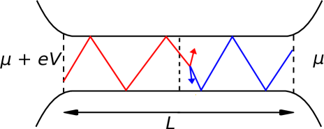
Figure 1: A sketch of the ballistic multimode wire with two electrons colliding half-way. The collision of the left-moving electron (blue) with the right-moving one (red) prevents the left-mover from crossing the section of the wire shown by the dashed line in the middle and therefore affects the current flowing through it despite the momentum conservation.

II Model and basic equations

Consider a metallic wire of uniform cross-section connecting two massive electronic reservoirs. The length $L$ of the wire is much larger than its transverse dimension $a$ but much smaller than both the elastic and inelastic mean free paths. In its turn, $a$ is much larger than the Fermi wavelength $\lambda_{F}$. It is assumed that electrons are specularly reflected at the boundaries of the wire, so they cannot transfer their longitudinal momentum to the lattice. In a two-dimensional (2D) case, such a wire could be realized by twisting up a 2D conducting strip to form a tube so that the boundary scattering could be eliminated at all. We neglect here the effects of electron-electron scattering near the contacts of the wire with the reservoirs Nagaev08 ; Nagaev10 . The kinetic equation for the distribution function of electrons inside the wire is of the form Lunde06

$${\bf v}\,\frac{\partial f}{\partial{\bf r}}=\hat{I}_{ee},$$ (1)

where the collision integral is given by

$$\hat{I}_{ee}({\bf p})=\alpha_{ee}\,\nu_{d}^{-2}\int\frac{d^{d}k}{(2\pi)^{d}}\int\frac{d^{d}p^{\prime}}{(2\pi)^{d}}\int d^{d}k^{\prime}\,\\ {}\times\delta({\bf p}+{\bf k}-{\bf p}^{\prime}-{\bf k}^{\prime})\,\delta(\varepsilon_{{\bf p}}+\varepsilon_{{\bf k}}-\varepsilon_{{\bf p}^{\prime}}-\varepsilon_{{\bf k}^{\prime}})\\ {}\times\Bigl{\{}[1-f({\bf p})]\,[1-f({\bf k})]\,f({\bf p}^{\prime})\,f({\bf k}^{\prime})\,\\ {}-f({\bf p})\,f({\bf k})\,[1-f({\bf p}^{\prime})]\,[1-f({\bf k}^{\prime})]\Bigr{\}},$$ (2)

$\alpha_{ee}$ is the dimensionless interaction parameter, $d=2$ or 3 is the dimensionality of the system; $\nu_{3}=mp_{F}/\pi^{2}$ and $\nu_{2}=m/\pi$ are the three- and two-dimensional two-spin electronic densities of states ($\hbar=1$). The term with electric field is omitted because we address the linear response and the voltage drop is included in the boundary conditions

$$f(p_{x}>0,x=0) =f_{R}(\varepsilon_{{\bf p}}-E_{F}),$$ (3)

$$f(p_{x}<0,x=L) =f_{L}(\varepsilon_{{\bf p}}-E_{F}),$$ (4)

where $x$ is the longitudinal coordinate, $f_{R}(\varepsilon)=f_{0}(\varepsilon-eV)$ and $f_{L}(\varepsilon)=f_{0}(\varepsilon)=1/[1+\exp(\varepsilon/T)]$. The current through an arbitrary section of the conductor is given by an integral over the transverse coordinates

$$I=2e\int d^{d-1}r_{\perp}\,\int\frac{d^{d}p}{(2\pi)^{d}}\,v_{x}\,f({\bf p},x,{\bf r}_{\perp}).$$ (5)

Equation (1) may be solved iteratively in the collision integral. In the zero approximation, the electrons move inside the wire along broken lines while retaining their energy and longitudinal momentum (see Fig. 1), so their distribution depends solely on the reservoir from which the trajectory of an electron with a given momentum originates. Therefore the coordinate-independent distribution is of the form

$$f^{(0)}({\bf p},{\bf r})=\Theta(p_{x})\,f_{R}(\varepsilon_{{\bf p}}-E_{F})\\ {}+\Theta(-p_{x})\,f_{L}(\varepsilon_{{\bf p}}-E_{F})$$ (6)

and the zero-approximation two-spin conductance is just given by the Sharvin formula Sharvin ; Kulik77

$$G_{03}=\frac{e^{2}a^{2}p_{F}^{2}}{4\pi^{2}},\qquad G_{02}=\frac{e^{2}p_{F}a}{\pi^{2}}.$$ (7)

To the first approximation in $\alpha_{ee}$, the correction to the distribution function $\delta f({\bf p},{\bf r})$ at a given point ${\bf r}$ of the conductor is readily obtained by integrating $\hat{I}_{ee}\{f^{(0)}\}$ along the trajectory of an electron with momentum ${\bf p}$ that comes to point ${\bf r}$ from the corresponding reservoir. As $\hat{I}_{ee}\{f^{(0)}\}$ is coordinate-independent, this integration is reduced to multiplying it by the time of motion inside the conductor

$$\delta f(p_{x}>0,{\bf p}_{\perp},x)=\frac{x}{v_{x}}\,\hat{I}_{ee}(p_{x}>0,|p_{\perp}|),$$ (8)

$$\delta f(p_{x}<0,{\bf p}_{\perp},x)=\frac{L-x}{|v_{x}|}\,\hat{I}_{ee}(p_{x}<0,|p_{\perp}|).$$ (9)

Upon a substitution of Eqs. (8) and (9) into Eq. (5) $v_{x}$ nicely drops off and taking into account the particle-number conservation by the collision integral, one obtains an expression similar to that of Lunde07

$$\delta I=2eLa^{d-1}\int\frac{d^{d}p}{(2\pi)^{d}}\,\Theta(p_{x})\,\hat{I}_{ee}({\bf p}),$$ (10)

which tells us that $\delta I$ is proportional to the rate of change in the number of electrons with $p_{x}>0$. One might think that it contradicts the momentum-conservation law, but this is not the case. Though collisions between electrons do not change their total momentum, they change their trajectories and hence may prevent some of them from passing through the cross-section of the conductor at which the current is calculated (see Fig. 1).

Equation (8) must be substituted into (10). Because of a piecewise distribution (6), it is convenient to present the result as a sum of integrals over left-moving and right-moving electronic states. Upon a decomposition of momentum integration into the integrations over the angles and over the energies, one obtains

$$\delta I=2\frac{ea^{d-1}L\alpha_{ee}}{\nu_{d}^{2}}\sum_{\alpha\beta\gamma=(L,R)}\int d\varepsilon\int d\varepsilon^{\prime}\int d\varepsilon_{1}\int d\varepsilon_{2}\,\\ {}\times\delta(\varepsilon+\varepsilon^{\prime}-\varepsilon_{1}-\varepsilon_{2})\\ {}\times F_{R\alpha\beta\gamma}(\varepsilon,\varepsilon^{\prime}|\varepsilon_{1},\varepsilon_{2})\,B_{R\alpha\beta\gamma}(\varepsilon,\varepsilon^{\prime}|\varepsilon_{1},\varepsilon_{2}),$$ (11)

where the indices $\alpha$, $\beta$, and $\gamma$ correspond to left-moving (L) and right-moving (R) states. The distribution-dependent factor is given by

$$F_{R\alpha\beta\gamma}(\varepsilon,\varepsilon^{\prime}|\varepsilon_{1},\varepsilon_{2})\\ =[1-f_{R}(\varepsilon)]\,[1-f_{\alpha}(\varepsilon^{\prime})]\,f_{\beta}(\varepsilon_{1})\,f_{\gamma}(\varepsilon_{2})\,\\ {}-f_{R}(\varepsilon)\,f_{\alpha}(\varepsilon^{\prime})\,[1-f_{\beta}(\varepsilon_{1})]\,[1-f_{\gamma}(\varepsilon_{2})]$$ (12)

with $f_{R}(\varepsilon)=f_{0}(\varepsilon-eV)$ and $f_{L}(\varepsilon)=f_{0}(\varepsilon)$. The quantity

$$B_{R\alpha\beta\gamma}(\varepsilon,\varepsilon^{\prime}|\varepsilon_{1},\varepsilon_{2})=\int\frac{d^{d}p}{(2\pi)^{d}}\int\frac{d^{d}k}{(2\pi)^{d}}\int\frac{d^{d}p^{\prime}}{(2\pi)^{d}}\\ {}\times\int d^{2}k^{\prime}\,\delta(\varepsilon_{{\bf p}}-E_{F}-\varepsilon)\,\delta(\varepsilon_{{\bf k}}-E_{F}-\varepsilon^{\prime})\,\\ {}\times\delta(\varepsilon_{{\bf p}}^{\prime}-E_{F}-\varepsilon_{1})\,\delta(\varepsilon_{{\bf k}}^{\prime}-E_{F}-\varepsilon_{2})\Theta(p_{x})\,\Theta(\sigma_{\alpha}\,k_{x})\,\\ {}\times\Theta(\sigma_{\beta}\,p^{\prime}_{x})\,\Theta(\sigma_{\gamma}\,k^{\prime}_{x})\,\delta({\bf p}+{\bf k}-{\bf p}^{\prime}-{\bf k}^{\prime})$$ (13)

with $\sigma_{R}=1$ and $\sigma_{L}=-1$ is the factor representing the phase space available for scattering. The quantity $B_{RRLL}$ is zero because of momentum conservation, and the distribution-dependent factors $F_{RRRR}$, $F_{RLRL}$, and $F_{RLLR}$ vanish because of energy conservation. Hence only four terms in the sum (11) containing odd numbers of left-moving and right-moving states are nonzero. Note that $B_{\alpha\beta\gamma\delta}$ is symmetric with respect to permutations of the first and second pairs of arguments and to permutations inside these pairs and also symmetric with respect to a simulataneous reversal of all its indices. Using these symmetry properties and linearizing $F_{R\alpha\beta\gamma}$ with respect to the voltage, one may reduce the sum (11) to a single term

$$\delta I=-4\frac{ea^{d-1}L\alpha_{ee}}{\nu_{d}^{2}}\,\frac{eV}{T}\int d\varepsilon\int d\varepsilon^{\prime}\int d\varepsilon_{1}\int d\varepsilon_{2}\,\\ {}\times\delta(\varepsilon+\varepsilon^{\prime}-\varepsilon_{1}-\varepsilon_{2})\,\tilde{F}(\varepsilon,\varepsilon^{\prime}|\varepsilon_{1},\varepsilon_{2})B(\varepsilon,\varepsilon^{\prime}|\varepsilon_{1},\varepsilon_{2}),$$ (14)

where

$$\tilde{F}(\varepsilon,\varepsilon^{\prime}|\varepsilon_{1},\varepsilon_{2})=[1-f_{0}(\varepsilon)]\,[1-f_{0}(\varepsilon^{\prime})]\,\\ {}\times f_{0}(\varepsilon_{1})\,f_{0}(\varepsilon_{2}).$$ (15)

The quantity $B\equiv B_{RRRL}$ exhibits different behaviors for $d=3$ and $d=2$. In the three-dimensional case, it is dominated by collisions of electrons with total momentum $\bf Q$ of the order of $p_{F}$ and remains finite even if all the initial and final states lie exactly at the Fermi surface. This may be understood as follows. Consider two electrons with momenta ${\bf p}$ and ${\bf k}$ lying exactly on the Fermi sphere that scatter into ${\bf p}^{\prime}$ and ${\bf k}^{\prime}$, respectively. Because of the conservation laws, the two initial and the two final states form a rectangle inscribed in the sphere and lying in a plane perpendicular to $\bf Q$, which is located at a distance $Q/2$ from its center (see Fig. 2). Depending on the direction and length of $\bf Q$, the plane $p_{x}=0$ may cut the rectangle into two parts and isolate two, one, or none of the vertices from it. The quantity $B_{RRRL}$ is determined by momentum configurations with just one isolated vertex, which exist even in the zero-energy limit. To the lowest order in $\varepsilon$, calculations give (see Appendix A) $B=C_{3}\,m^{4}p_{F}$ where $C_{3}=0.222$, and the relative correction to the conductance is

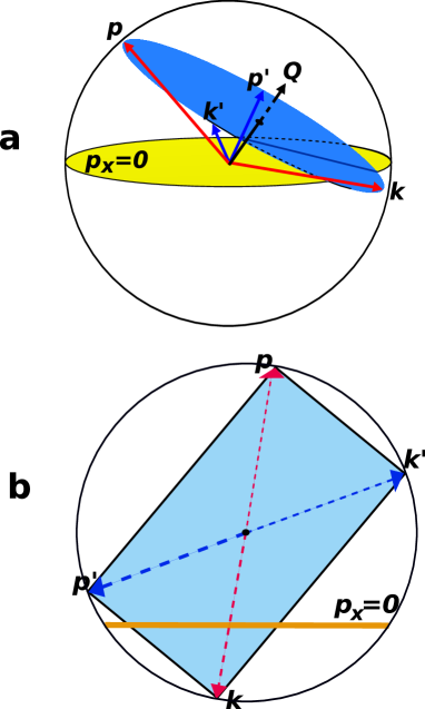
Figure 2: A 3D Fermi surface and the four states involved in a collision of two electrons. States ${\bf p}$, ${\bf p}^{\prime}$ and ${\bf k}^{\prime}$ correspond to electrons moving from left to right whereas state ${\bf k}$ corresponds to an opositely moving electron. (a) A 3D view of the Fermi sphere and (b) its section with the plane containing the four states with the trace of the plane $p_{x}=0$ (yellow line). The collision increases the number of right-movers by one.

$$\frac{\delta G_{3}}{G_{03}}=-\frac{C_{3}}{3}\,\frac{L}{v_{F}}\,\frac{\alpha_{ee}T^{2}}{E_{F}}\sim-\frac{L}{l_{ee}},$$ (16)

where $l_{ee}$ is the standard length of electron-electron scattering. This means that a significant proportion of electron–electron collision contributes to the current.

In the two-dimensional case, $B$ vanishes at $\varepsilon=\varepsilon^{\prime}=\varepsilon_{1}=\varepsilon_{2}=0$, and therefore the correction to the current is determined by collisions with small total momenta. Explicit calculations give (see Appendix B)

$$B(\varepsilon,\varepsilon^{\prime}|\varepsilon_{1},\varepsilon_{2})=\frac{\sqrt{2}m^{3/2}T^{1/2}}{16\pi^{6}v_{F}^{3}}\,S\!\left(\frac{\varepsilon-\varepsilon^{\prime}}{2T},\frac{\varepsilon_{1}-\varepsilon_{2}}{2T}\right)\!,$$ (17)

where

$$S(x,y)=\begin{cases}\sqrt{|x|+y}+\sqrt{y-|x|},&y>|x|\\ \sqrt{|x|+y},&|y|<|x|\\ 0,&y<-|x|.\end{cases}$$ (18)

The difference from the three-dimensional case is readily seen in Fig. 3. All the four momenta may lie exactly at the Fermi circle only at ${\bf Q}=0$. In that case, the center of the rectangle coincides with the center of the Fermi circle and the line $p_{x}=0$ cuts it into two equal parts so that two vertices lie in the half-plane $p_{x}>0$ and the other two, in the half-plane $p_{x}<0$. If the four momenta are located within $\delta\varepsilon\sim T$ from the Fermi surface, a rectangle with one isolated vertex may be placed in this ring-shaped region only if all its vertices are located near the line $p_{x}=0$, where the portions of the ring at the opposite sides of the Fermi surface are almost parallel. Therefore characteristic values of $Q$ that dominate $B$ are determined by the length at which the bending of these portions is of the order of their width $\delta\varepsilon/v_{F}$, i.e. $Q\sim\sqrt{p_{F}\varepsilon/v_{F}}$. A substitution of Eqs. (17) and (18) into (14) gives

$$\frac{\delta G_{2}}{G_{02}}=-\frac{C_{2}}{2\pi^{2}}\,\frac{L}{v_{F}}\,\frac{\alpha_{ee}T^{5/2}}{E_{F}^{3/2}},$$ (19)

where $C_{2}=2.23$. This suggests that at low temperatures, $\delta G_{2}/G_{02}$ is smaller than $L/l_{ee}$ by a factor $(T/E_{F})^{1/2}$ and only a small fraction of electron–electron collisions affects the current.

The proportionality of $\delta G_{3}$ and $\delta G_{2}$ to $L$ is the result of the linear approximation in $\alpha_{ee}$. In fairly long wires, this approximation breaks down. It is reasonable to believe that at $L\to\infty$ the corrections to the conductance saturate to a finite value as is in the case of a single-mode channel Micklitz10 and therefore present a boundary effect.

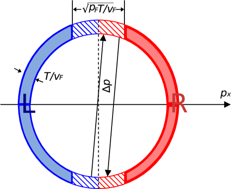
Figure 3: A 2D Fermi surface and a scattering process that changes the number of right-moving electrons. The dashed areas show the parts of the surface that contribute to such processes.

III Discussion

In contrast to the positive contribution to the conductance from the scattering in short and wide ballistic contacts MacDonald82 ; Nagaev08 ; Nagaev10 , the negative contribution in long and narrow wires does not require an explicit transfer of electron momentum to a macroscopic obstacle. Instead, the excess momentum is absorbed in the reservoirs just like the energy of injected electrons. The principal difference from the case of short contacts is that the collisions in a long and narrow channel involve only two type of electrons, left-movers and right-movers,which both contribute to the current with opposite signs. In contrast to this, in wide and short contacts the collisions involve also a third type of electrons, by-passers. They by far outnumber the first two types, do not contribute to the current in the absence of scattering but can be converted into a left-mover or right-mover upon a collision.

The scattering mechanism in wires is more efficient in 3D than in 2D because the fraction of collisions contributing to the current increases with the dimensionality. Unlike this, the scattering contribution in wide contacts is smaller in 3D than in 2D because the concentration of injected nonequilibrium electrons falls off faster in 3D reservoirs.

The scattering contribution to the resistance may be well observable in GaAs heterostructures under realistic experimental condition. For an electronic density $n_{s}=10^{11}$ cm^-2 and $T=4$ K high-mobility samples may have the elastic mean free path as large as 20 $\mu m$. For a conducting channel of that length and $\alpha_{ee}\sim 1$, the correction to the conductance should be about 10%. This correction can be isolated from the noninteracting Sharvin resistance (7) by changing the length of the channel $L$ in a 2D electron gas by means of electrostatic gates and isolating the component of the resistance proportional to $L$.

IV Summary

In summary, we have shown that two-electron collisions contribute to the electric resistivity of multimode finite-length metallic wires even in the absence of umklapp processes. The finite contribution to the resistivity is due to the breaking of translational symmetry of the system by the presence of reservoirs. This effect has a power-law temperature dependence and is more pronounced in 3D wires than in 2D ones.

Appendix A Calculation of $B$ for the 3D case

The phase space available for scattering (13) may be rewritten in a form

$$B(\varepsilon,\varepsilon^{\prime}|\varepsilon_{1},\varepsilon_{2})=\int\frac{d^{d}Q}{(2\pi)^{d}}\,A_{RR}(\varepsilon,\varepsilon^{\prime},{\bf Q})\\ {}\times A_{RL}(\varepsilon_{1},\varepsilon_{2},{\bf Q}),$$ (20)

where ${\bf Q}={\bf p}+{\bf k}={\bf p}^{\prime}+{\bf k}^{\prime}$ is the total momentum of the colliding electrons and

$$A_{\alpha\beta}(\varepsilon,\varepsilon^{\prime},{\bf Q})=\frac{1}{(2\pi)^{d}}\int d^{d}p\int d^{d}k\,\Theta(\sigma_{\alpha}\,p_{x})\,\Theta(\sigma_{\beta}\,k_{x})\,\\ {}\times\delta(\varepsilon_{{\bf p}}-E_{F}-\varepsilon)\,\delta(\varepsilon_{{\bf k}}-E_{F}-\varepsilon^{\prime})\,\delta({\bf p}+{\bf k}-{\bf Q}).$$ (21)

In 3D, explicit calculations give

$$A_{RR}(\varepsilon,\varepsilon^{\prime},{\bf Q})\\ =\frac{2m^{2}}{(2\pi)^{3}Q}\,\Theta(\Delta)\int\limits_{0}^{\pi}d\varphi\,\Theta\!\left(\frac{Q_{x}}{Q_{\perp}}\,\frac{p^{2}_{\varepsilon}-p^{2}_{\varepsilon^{\prime}}+Q^{2}}{\sqrt{\Delta(Q,\varepsilon,\varepsilon^{\prime})}}-\cos\varphi\right)\\ {}\times\Theta\!\left(\cos\varphi-\frac{Q_{x}}{Q_{\perp}}\,\frac{p^{2}_{\varepsilon}-p^{2}_{\varepsilon^{\prime}}-Q^{2}}{\sqrt{\Delta(Q,\varepsilon,\varepsilon^{\prime})}}\right)$$ (22)

and

$$A_{RL}(\varepsilon,\varepsilon^{\prime},{\bf Q})=\frac{2m^{2}}{(2\pi)^{3}Q}\,\Theta(\Delta)\\ {}\times\int\limits_{0}^{\pi}d\varphi\,\Theta\!\left(\frac{Q_{x}}{Q_{\perp}}\,\frac{p^{2}_{\varepsilon}-p^{2}_{\varepsilon^{\prime}}-Q^{2}}{\sqrt{\Delta(Q,\varepsilon,\varepsilon^{\prime})}}-\cos\varphi\right),$$ (23)

where $p_{\varepsilon}=\sqrt{2m(\varepsilon+E_{F})}$, $p_{\varepsilon^{\prime}}=\sqrt{2m(\varepsilon^{\prime}+E_{F})}$, and

$$\Delta(Q,\varepsilon,\varepsilon^{\prime})=\Bigl{[}Q^{2}-(p_{\varepsilon}-p_{\varepsilon^{\prime}})^{2}\Bigr{]}\,\\ {}\times\Bigl{[}(p_{\varepsilon}+p_{\varepsilon^{\prime}})^{2}-Q^{2}\Bigr{]}.$$ (24)

The calculations are greatly simplified if $\varepsilon-\varepsilon^{\prime}\to 0$. By going to spherical coordinates in (20) and introducing new integration variables $u=Q/2p_{F}$ and $v=Q^{2}\,\Delta^{-1/2}\cot\theta$ instead of the radial coordinate $Q$ and the polar angle $\theta$, one arrives at an expression $B=C_{3}\,m^{4}p_{F}$, where

$$C_{3}=\frac{1}{2^{4}\pi^{8}}\int\limits_{0}^{1}du\,u^{2}\,\sqrt{1-u^{2}}\\ {}\times\int\limits_{0}^{1}dv\,\frac{\arcsin v\,\arccos v}{(u^{2}+v^{2}-u^{2}v^{2})^{3/2}}=0.222.$$ (25)

Appendix B Calculation of $B$ for the 2D case

Equations (20) and (21) are also valid in the 2D case, but the explicit expressions for $A_{RR}$ and $A_{RL}$ are now of the form

$$A_{RR}(\varepsilon,\varepsilon^{\prime},{\bf Q})=\frac{m^{2}}{2\pi^{2}}\,\frac{\Theta(\Delta)}{\sqrt{\Delta(Q,\varepsilon,\varepsilon^{\prime})}}\\ {}\times\Bigl{\{}\Theta\!\Bigl{[}(Q^{2}+p_{\varepsilon}^{2}-p_{\varepsilon^{\prime}}^{2})\,Q_{x}+|Q_{y}|\,\sqrt{{\Delta(Q,\varepsilon,\varepsilon^{\prime})}}\Bigr{]}\\ {}\times\Theta\!\Bigl{[}(Q^{2}-p_{\varepsilon}^{2}+p_{\varepsilon^{\prime}}^{2})\,Q_{x}-|Q_{y}|\,\sqrt{{\Delta(Q,\varepsilon,\varepsilon^{\prime})}}\Bigr{]}\\ {}+\Theta\!\Bigl{[}(Q^{2}+p_{\varepsilon}^{2}-p_{\varepsilon^{\prime}}^{2})\,Q_{x}-|Q_{y}|\,\sqrt{{\Delta(Q,\varepsilon,\varepsilon^{\prime})}}\Bigr{]}\,\\ {}\times\Theta\!\Bigl{[}(Q^{2}-p_{\varepsilon}^{2}+p_{\varepsilon^{\prime}}^{2})\,Q_{x}+|Q_{y}|\,\sqrt{{\Delta(Q,\varepsilon,\varepsilon^{\prime})}}\Bigr{]}\Bigr{\}},$$ (26)

$$A_{RL}(\varepsilon_{1},\varepsilon_{2},{\bf Q})=\frac{m^{2}}{2\pi^{2}}\,\frac{\Theta(\Delta)}{\sqrt{\Delta(Q,\varepsilon_{1},\varepsilon_{2})}}\\ {}\times\Bigl{\{}\Theta\!\Bigl{[}(Q^{2}+p_{\varepsilon 1}^{2}-p_{\varepsilon 2}^{2})\,Q_{x}+|Q_{y}|\,\sqrt{{\Delta(Q,\varepsilon_{1},\varepsilon_{2})}}\Bigr{]}\\ {}\times\Theta\!\Bigl{[}(p_{\varepsilon 1}^{2}-p_{\varepsilon 2}^{2}-Q^{2})\,Q_{x}+|Q_{y}|\,\sqrt{{\Delta(Q,\varepsilon_{1},\varepsilon_{2})}}\Bigr{]}\\ {}+\Theta\!\Bigl{[}(Q^{2}+p_{\varepsilon 1}^{2}-p_{\varepsilon 2}^{2})\,Q_{x}-|Q_{y}|\,\sqrt{{\Delta(Q,\varepsilon_{1},\varepsilon_{2})}}\Bigr{]}\,\\ {}\times\Theta\!\Bigl{[}(p_{\varepsilon 1}^{2}-p_{\varepsilon 2}^{2}-Q^{2})\,Q_{x}\\ {}-|Q_{y}|\,\sqrt{{\Delta(Q,\varepsilon_{1},\varepsilon_{2})}}\Bigr{]}\Bigl{\}}.$$ (27)

The integral (20) is conveniently calculated by going to radial coordinates. As Eqs. (26) and (27) depend on the $|Q_{y}|/Q_{x}$ ratio only through $\Theta$-functions, it takes up a form

$$B(\varepsilon,\varepsilon^{\prime}|\varepsilon_{1},\varepsilon_{2})\\ {}=\frac{m^{4}}{16\pi^{6}}\int\limits_{0}^{2p_{F}}dQ\,\frac{Q\,\delta\varphi(Q)}{\sqrt{\Delta(Q,\varepsilon,\varepsilon^{\prime})\,\Delta(Q,\varepsilon_{1},\varepsilon_{2})}},$$ (28)

where $\delta\varphi(Q)$ is the angular width of the domain of integration defined by the theta-functions in Eqs. (26) and (27). The integral is dominated by small values of $Q\sim\sqrt{p_{F}\varepsilon/v_{F}}\ll p_{F}$, so that

$$\Delta(Q,\varepsilon,\varepsilon^{\prime})\approx\Delta(Q,\varepsilon_{1},\varepsilon_{2})\approx 4p_{F}^{2}Q^{2}.$$ (29)

The integration results in Eqs. (17) and (18).

References

- (1) R. Peierls, Ann. Phys. (Leipzig) 395, 1055 (1929).
- (2) B. L. Altshuler and A. G. Aronov, in Electron-electron Interactions in Disordered Systems, edited by A. L. Efros and M. Pollak (North-Holland, Amsterdam, 1985), p. 1.
- (3) G. Zala, B. N. Narozhny, and I. L. Aleiner, Phys. Rev. B 64, 214204 (2001).
- (4) See M. J. M. de Jong and L. W. Molenkamp, Phys. Rev. B 51, 13389 (1995) and references therein.
- (5) A. H. MacDonald and C. R. Leavens, J. Phys. F 12, 2323 (1982).
- (6) K. E. Nagaev and O. S. Ayvazyan, Phys. Rev. Lett. 101, 216807 (2008).
- (7) K. E. Nagaev and T. V. Kostyuchenko, Phys. Rev. B 81, 125316 (2010).
- (8) A.M. Lunde, A. De Martino, A. Schulz, R. Egger, and K. Flensberg, New Journal of Physics 11, 023031 (2009)
- (9) A. M. Lunde, K. Flensberg, and L. I. Glazman, Phys. Rev. Lett. 97, 256802 (2006).
- (10) A. M. Lunde, K. Flensberg, and L. I. Glazman, Phys.Rev. B 75, 245418 (2007).
- (11) T. Micklitz, J. Rech, and K. A. Matveev, Phys. Rev. B 81, 115313 (2010).
- (12) A. Levchenko, T. Micklitz, J. Rech, and K. A. Matveev, Phys. Rev. B 82, 115413 (2010).
- (13) A. Levchenko, Z. Ristivojevic, and T. Micklitz, Phys. Rev. B 83, 041303 (2011)
- (14) Y. V. Sharvin, Zh. Eksp. Teor. Fiz. 48, 984 (1965) [Sov. Phys. JETP 21, 655 (1965)].
- (15) Kulik, Shekhter, and Omelyanchouk, Solid State Comm. 23, 301 (1977); Kulik, Omel’yanchuk, and Shekhter, Fiz. Nizk. Temp. 3, 1543-1558 (1977) [Sov. J. Low Temp. Phys. 3, 740 (1977)].