Computing equilibrium concentrations for large hetero-dimerization networks

Abstract

We consider a chemical reaction network governed by mass action kinetics and composed of $N$ different species which can reversibly form heterodimers. A fast iterative algorithm is introduced to compute the equilibrium concentrations of such networks. We show that the convergence is guaranteed by the Banach fixed point theorem. As a practical example, of relevance for a quantitative analysis of microarray data, we consider a reaction network formed by $N\sim 10^{6}$ mutually hybridizing different mRNA sequences. We show that, despite the large number of species involved, the convergence to equilibrium is very rapid for most species. The origin of slow convergence for some specific subnetworks is discussed. This provides some insights for improving the performance of the algorithm.

I Introduction

Systems of coupled chemical reactions involving many different species, i.e. reaction networks, have been intensively studied in chemistry, physics, mathematics, and engineering sciences (see e.g. fein87 ; dejo02 ; gerd04 ; conr05 ; alon06 ; mart10 ; shin10 ; zwic10 ; pant10 ; mill11 ). If diffusion is fast enough and the number of molecules is sufficiently large, so that stochastic effects can be neglected, these systems can be described by a set of coupled first order ordinary differential equations (ODE), which govern the time evolution of the concentrations of each species. In the ODE description, the rates of production and consumption of the chemical species are given in term of mass action, Michaelis-Menten, or other cooperative-type kinetics dejo02 . In such systems different types of behavior are possible, as for instance relaxation to a unique stationary point, oscillations or multistability.

Usually the time evolution of the system can be computed through numerical integration of the ODE. However, this method can become very slow for large reaction networks. In addition, the main interest is typically the long time behavior of the system, which in absence of oscillations boils down to finding the stationary (equilibrium) concentrations of each of the chemical species.

In the present work, we will describe an efficient method to find equilibrium concentrations for a class of networks which we will refer to as hetero-dimerization networks. In these networks the species associate to form dimers, which eventually break apart giving back the single species. The method is based on an iterative scheme, of which we can rigorously prove the convergence. The proof relies on the Banach fixed point theorem.

The proposed method is very efficient for large reaction networks. As an example to show that convergence is fast, even for systems with $\sim 10^{6}$ species, we consider the hybridization of RNA strands. This example is of relevance, for instance, for a better quantitative understanding of the reactions underlying the functioning of DNA microarrays carl06 ; bind06 ; burd06 ; halp06 . It shows that some sequences tend to get effectively depleted from the solution because of partial complementarity with other strands. This brings some consequences for the design and interpretation of microarray experiments.

This paper is organized as follows. In Section II we introduce the iterative algorithm and prove its convergence to the fixed point, irrespective of the initial condition. In Section III we show a concrete calculation for a network composed of a large number of hybridizing mRNA strands. Section IV discusses the convergence rate of the algorithm and Section V concludes the paper.

II Hetero-dimerization reactions

II.1 Iterative scheme for stationary point

We consider a set of different chemical species $A_{i}$ ($i=1,2\ldots N$) undergoing reversible association/dissociation reactions of the type:

$$A_{i}+A_{j}\autorightleftharpoons{K_{ij}}{\overline{K}_{ij}}A_{ij}.$$ (1)

where $K_{ij}$ and $\overline{K}_{ij}$ are the forward and reverse rates. The ratio of the rates must satisfy the detailed balance condition

$$K_{ij}/\overline{K}_{ij}=e^{\Delta G_{ij}/RT}$$ (2)

where $\Delta G_{ij}$ is the free energy of formation of the complex $A_{ij}$ (the free energy difference between the bound and unbound state).

The system is considered to be well-mixed, i.e. diffusion of all species is assumed to occur on a fast time scale compared to reaction time scales. Furthermore, production and degradation are assumed to be absent. A configuration can then be characterised solely by the concentrations of all species $c_{i}$ and of all dimers $c_{ij}$ at a given time. In addition, the following conservation laws hold for every species $A_{i}$:

$$\overline{c}_{i}=c_{i}+\sum_{j}c_{ij}$$ (3)

with $\overline{c}_{i}$ the constant total concentration of a species.

We consider mass-action kinetics, so the concentrations evolve in time according to

$$\frac{{\rm d}c_{i}}{{\rm d}t}=\sum_{j}\overline{K}_{ij}c_{ij}-\sum_{j}K_{ij}c_{i}c_{j},$$ (4)

and we are interested in the stationary solution ${\rm d}c_{i}/{\rm d}t=0$. A general theorem on Mass Action Reaction Networks, the so-called Deficiency Zero Theorem fein87 , guarantees that the system (1) has a unique stationary point, irrespective of the values of ${K}_{ij}$ and $\overline{K}_{ij}$. We omit the proof of this statement, it amounts to calculating the deficiency of the reaction network, which is an integer easily obtainable from the network topology (for more details see fein87 ). Given a set of rates $\overline{K}_{ij}$ and $K_{ij}$ and some initial concentrations, it is always possible to compute the relaxation to equilibrium by solving the ODE in Eq. (4) numerically, for instance through discretization in small time steps $\Delta t$. However, this is a very costly procedure and thus very unpractical for large networks. In addition the discretization brings some errors scaling as powers of $\Delta t$, which accumulate during the calculation. We show here that the problem of finding the stationary point can be reformulated as an iterative problem, which is much more efficient and does not involve discretization approximations.

The detailed balance condition (Eq. (2)) provides some freedom in choosing the forward and reverse rates. Only their ratio needs to be fixed to guarantee convergence to the stationary point. One particularly interesting choice is $\overline{K}_{ij}=1$, and thus $K_{ij}=e^{\Delta G_{ij}/RT}$. Substituting these values in Eq.(4) while setting ${\rm d}c_{i}/{\rm d}t=0$ and using Eq. (3) one finds:

$$\overline{c}_{i}-c_{i}-\sum_{j}e^{\Delta G_{ij}/RT}c_{i}c_{j}=0$$ (5)

which we rewrite as

$$c_{i}=\frac{\overline{c}_{i}}{1+\sum_{j}e^{\Delta G_{ij}/RT}c_{j}}\equiv T_{i}(c_{1},\ldots c_{N}).$$ (6)

where the right hand side defines a function $T$ from the N-dimensional space of concentrations $\vec{c}=(c_{1},\ldots c_{N})$ into itself.

Equations (6) are a set of $N$ non-linear equations which must be solved to find the $c_{i}$. Using vector notation we write Eq. (6) as $\vec{c}=\vec{T}(\vec{c})$. A possible way to solve this set is to use an iterative approach. Starting from an initial guess $\vec{c}^{\,(0)}$, one can repeatedly apply the map $\vec{T}$ to obtain $\vec{c}^{\,(1)}=\vec{T}(\vec{c}^{\,(0)})$, …, $\vec{c}^{\,(k+1)}=\vec{T}(\vec{c}^{\,(k)})$, but it remains to be proven that the process converges to the fixed point. Indeed, the convergence in time to a unique stable fixed point of the kinetic equations (4) (according to the Zero Deficiency Theorem) does not a priori imply the convergence of the iterated map. However, this convergence is guaranteed by a fixed point theorem for iterated maps, which we discuss next.

II.2 Contraction maps

The Banach fixed-point theorem gran03 guarantees the existence and uniqueness of fixed points for a class of maps $\vec{c}\mapsto\vec{T}(\vec{c})$ of a metric space into itself. A map is said to be a contraction map if any pair of arbitrary points is mapped to a pair of points that are closer to each other, i.e. if for any two given points $\vec{c}$ and $\vec{c}{\,{}^{\prime}}$ in some subset $\Omega$ of a metric space for which $\vec{T}:\Omega\to\Omega$, one has:

$$d(\vec{T}(\vec{c}),\vec{T}(\vec{c}{\,{}^{\prime}}))\leq q\,d(\vec{c},\vec{c}{\,{}^{\prime}})$$ (7)

with $d$ the metric (distance function) on the metric space, and with a so-called Lipschitz constant $q<1$.

In order to prove that a map is a contraction one has to construct a suitable distance. Indeed, a map can be a contraction according to one distance, but not according to another one. We illustrate this from a simple one-dimensional example. Let us thus consider the map of the interval $[0,\overline{c}]$ into itself defined by

$$T(c)=\frac{\overline{c}}{1+Kc}$$ (8)

where $\overline{c}>0$ and $K>0$. This map has a unique fixed point since the quadratic equation $c(1+Kc)=\overline{c}$ has a single positive solution. In general this map is not a contraction for the usual Euclidean distance $d_{E}(a,b)\equiv|a-b|$. Take for instance $\overline{c}=2$, $K=1$ and $c=0.1$, $c^{\prime}=0.2$. One has $d_{E}(c,c^{\prime})=0.1$, whereas $d_{E}(T(c),T((c^{\prime}))=0.1515\ldots$, which shows that two points can be mapped further apart from each other.

We note that for any $c,c^{\prime}\geq 0$ one has

$$d_{E}(T(T(c)),T(T(c^{\prime})))=\left|\frac{\overline{c}}{1+\frac{K\overline{c}}{1+Kc}}-\frac{\overline{c}}{1+\frac{K\overline{c}}{1+Kc^{\prime}}}\right|$$ (9)

$$= \frac{K\overline{c}|c-c^{\prime}|}{(1+K(c+\overline{c}))(1+K(c^{\prime}+\overline{c}))}\leq q|c-c^{\prime}|$$

where

$$q=\frac{K\overline{c}}{(1+2K\overline{c})^{2}}<1$$ (10)

for any values of $K$ and $\overline{c}$. (9) and (10) together imply that $c\mapsto f(c)\equiv T(T(c))$ is a contraction map. Existence of a unique fixed point for contraction maps is guaranteed by the

Banach fixed point theorem - Let $(X,d)$ be a non-empty complete metric space. Furthermore, let $f:X\rightarrow X$ be a contraction mapping on $X$, i.e. there exists some $q<1$ (called the Lipschitz constant) such that $d(f(x),f(y))\leq q\,d(x,y)$ for all $x,y\in X$. Then the map $f$ has only one fixed point in $X$, and moreover, for any starting point $x_{0}\in X$, the sequence $\{x_{n}\}$ defined by $x_{n}=f(x_{n-1})$ converges towards this fixed point.

The problem with the Euclidean distance $d_{E}(\vec{x},\vec{x}^{\prime})=\sqrt{\sum_{i=1}^{N}(x_{i}-x_{i}^{\prime})^{2}}$ persists in higher dimensions, as it is possible to find $\vec{c}$, $\vec{c}^{\,\prime}$ for which $d_{E}(\vec{T}(\vec{c}),\vec{T}(\vec{c}^{\,\prime}))>d_{E}(\vec{c},\vec{c}^{\,\prime})$. Therefore, we chose a different strategy. To use the Banach fixed point theorem in higher dimension, we constructed an appropriate metric for which we can explicitly prove that the map $\vec{c}\mapsto\vec{T}(\vec{c})$ is a contraction. In the one dimensional case the metric is:

$$d(c,c^{\prime})=\frac{|c-c^{\prime}|}{c+c^{\prime}}$$ (11)

We prove later that this indeed defines a metric for its high-dimensional generalization, first we will consider the one-dimensional case. We note that the presence of the denominator in (11) may produce a singularity when $c,c^{\prime}\to 0$. To avoid this problem we restrict ourselves to the interval $X=[T(\overline{c}),\overline{c}]$. It can be shown easily that $T$ maps $X$ into itself and that $0<T(\overline{c})<\overline{c}$ so that the metric (11) is always well-defined. $X$ is also a compact space. Roughly speaking a space is compact if there are no points “missing” from it, either inside it or at the boundary. A close interval $[a,b]$ is compact. Also a rectangle or a cube in two and three dimensions are compact, provided all points in the borders are included. A hypercube, the $N$-dimensional analog of a cube, is also compact. Recall that given $N$ pairs of numbers $(a_{i},b_{i})$ (with $a_{i}<b_{i}$) a hypercube $X$ contains all points $(x_{1},x_{2},\ldots x_{N})$ such that $a_{i}\leq x_{i}\leq b_{i}$. We have

$$d(T(c),T(c^{\prime}))=\frac{K|c-c^{\prime}|}{2+K(c+c^{\prime})}$$ (12)

$$= \frac{K(c+c^{\prime})}{2+K(c+c^{\prime})}\,d(c,c^{\prime})\leq q\,d(c,c^{\prime})$$

where

$$q=\frac{K\overline{c}}{1+K\overline{c}}\leq 1$$ (13)

for any value of $K$ and $\overline{c}$. This shows that according to the metric (11) the map $c\mapsto T(c)$ is a contraction. In the following we will introduce a metric which is a higher dimensional generalization of (11).

II.3 Higher dimensional map

Consider any $N\times N$ matrix with non-negative entries ($K_{ij}\geq 0$). We prove that the map defined in Eq. (6) is a contraction in the space $X$ of $N$-dimensional vectors $\vec{c}=(c_{1},c_{2}\ldots c_{N})$ such that all elements are $\varepsilon_{i}\leq c_{i}\leq\overline{c_{i}}$, where $\overline{c_{i}}$ are fixed. Here we have defined

$$\varepsilon_{i}\equiv\frac{\overline{c_{i}}}{1+\sum_{j}K_{ij}\overline{c_{j}}}>0$$ (14)

It is easy to show that $\vec{T}$ maps $X$ into itself. $X$ is also compact.

We consider the metric defined as

$$d(\vec{c},\vec{c}{\,{}^{\prime}})=\max_{1\leq i\leq N}\frac{|c_{i}-c_{i}^{\prime}|}{c_{i}+c_{i}^{\prime}}$$ (15)

which is a higher dimensional generalization of (11). To prove that $\vec{T}$ is a contraction we have to show that for any two points in $X$, say $\vec{c}$ and $\vec{c}{\ {}^{\prime}}$, one has

$$d(\vec{T}(\vec{c}),\vec{T}(\vec{c}{\,{}^{\prime}}))\leq q\,d(\vec{c},\vec{c}{\,{}^{\prime}})$$ (16)

with Lipschitz constant $q<1$. We first show that (15) has the mathematical properties of a distance and then that (16) holds.

II.3.1 Eq. (15) defines a metric

To show that $d()$ as defined by Eq. (15) is a metric on the metric space $X$, we need to prove that for every $\vec{c}$, $\vec{c}{\,{}^{\prime}}$ and $\vec{c}{\,{}^{\prime\prime}}$ in $X$

• $d(\vec{c},\vec{c}{\,{}^{\prime}})\geq 0$ and $d(\vec{c},\vec{c}{\,{}^{\prime}})=0$ iff $\vec{c}=\vec{c}{\,{}^{\prime}}$

• $d(\vec{c},\vec{c}{\,{}^{\prime}})=d(\vec{c}{\,{}^{\prime}},\vec{c})$

• Triangle inequality: $d(\vec{c},\vec{c}{\,{}^{\prime}})\leq d(\vec{c},\vec{c}{\,{}^{\prime\prime}})+d(\vec{c}{\,{}^{\prime\prime}},\vec{c}{\,{}^{\prime}})$

Proof: a) and b) are trivial. The triangle inequality requires some more work. We need to prove that

$$\max_{i}\frac{|c_{i}-c^{\prime}_{i}|}{c_{i}+c^{\prime}_{i}}\leq\max_{i}\frac{|c_{i}-c^{\prime\prime}_{i}|}{c_{i}+c^{\prime\prime}_{i}}+\max_{i}\frac{|c^{\prime\prime}_{i}-c^{\prime}_{i}|}{c^{\prime\prime}_{i}+c^{\prime}_{i}},$$ (17)

We shall prove that the inequality holds for every $i$, thus that for any non-negative $a$, $b$ and $c$ one has

$$\frac{|a-b|}{a+b}\leq\frac{|a-c|}{a+c}+\frac{|c-b|}{c+b}.$$ (18)

First of all we note that the inequality (18) is satisfied when $a=0$ or $b=0$ or $c=0$. It is also satisfied when two elements are equal $a=b$, $a=c$ or $b=c$. We have to consider then these different cases: (1) $0<c<b<a$, (2) $0<c<a<b$, (3) $0<b<c<a$, (4) $0<b<a<c$, (5) $0<a<c<b$ and (6) $0<a<b<c$. However, the inequality (18) is symmetric in the exchange of $a$ with $b$. We have to prove it only for the cases for which $a>b$: (1) $0<c<b<a$, (3) $0<b<c<a$ and (4) $0<b<a<c$.

(1) $0<c<b<a$.

The inequality (18) becomes

$$\frac{a-b}{a+b}\leq\frac{a-c}{a+c}+\frac{b-c}{c+b}.$$ (19)

which, after some elementary algebra, can be rewritten as

$$(b-c)[2a(b+c)+(a+c)(a+b)]\geq 0$$ (20)

This inequality is verified in the case (1) since $b>c>0$ and $a>0$.

(3) $0<b<c<a$

The inequality (18) becomes

$$\frac{a-b}{a+b}\leq\frac{a-c}{a+c}+\frac{c-b}{c+b}$$ (21)

and after some simple algebra we get

$$(c-b)(a-c)(a-b)\geq 0$$ (22)

which is satisfied for $a>c>b>0$.

(4) $0<b<a<c$

The inequality (18) becomes

$$\frac{a-b}{a+b}\leq\frac{c-a}{a+c}+\frac{c-b}{c+b}$$ (23)

which can be rewritten as

$$(c-a)[2b(a+c)+(a+b)(c+b)]\geq 0$$ (24)

which is again satisfied for $c>a$.

This proves that the triangle inequality is satisfied. Hence $d$ defines a metric on $X$.

II.3.2 The inequality (16) is verified

Combining Eqs.(6) and (15) we find

$$d(\vec{T}(\vec{c}),\vec{T}(\vec{c}{\,{}^{\prime}})) = \max_{i}\frac{\left|\frac{\overline{c_{i}}}{1+\sum_{j}K_{ij}c_{j}}-\frac{\overline{c_{i}}}{1+\sum_{j}K_{ij}c_{j}^{\prime}}\right|}{\frac{\overline{c_{i}}}{1+\sum_{j}K_{ij}c_{j}}+\frac{\overline{c_{i}}}{1+\sum_{j}K_{ij}c_{j}^{\prime}}}$$ (25)

$$= \max_{i}\frac{\left|\sum_{j}K_{ij}(c_{j}-c_{j}^{\prime})\right|}{2+\sum_{j}K_{ij}(c_{j}+c_{j}^{\prime})}$$

$$\leq \max_{i}\frac{\sum_{j}K_{ij}\left|c_{j}-c_{j}^{\prime}\right|}{2+\sum_{j}K_{ij}(c_{j}+c_{j}^{\prime})}$$

To proceed further we make use of the inequality:

$$\frac{\sum_{l}a_{l}}{\sum_{l}b_{l}}\leq\max_{l}\left(\frac{a_{l}}{b_{l}}\right)$$ (26)

valid for $a_{l},b_{l}>0$. We prove this inequality in the case

$$\frac{a_{1}+a_{2}}{b_{1}+b_{2}}\leq\max\left(\frac{a_{1}}{b_{1}},\frac{a_{2}}{b_{2}}\right)$$ (27)

from which (26) follows easily by repeatedly applying (27). To verify (27) consider ${a_{1}}/{b_{1}}\geq{a_{2}}/{b_{2}}$. From this we have ${a_{1}}{b_{2}}\geq{a_{2}}{b_{1}}$ and ${a_{1}}{b_{2}}+{a_{1}}{b_{1}}\geq{a_{2}}{b_{1}}+{a_{1}}{b_{1}}$, which implies ${a_{1}}/{b_{1}}\geq(a_{1}+a_{2})/(b_{1}+b_{2})$ and proves (27).

Note that from (26) it is immediately clear that

$$\max_{i}\frac{\sum_{j}K_{ij}\left|c_{j}-c_{j}^{\prime}\right|}{2+\sum_{j}K_{ij}(c_{j}+c_{j}^{\prime})}\leq\max_{i}\frac{\sum_{j}K_{ij}\left|c_{j}-c_{j}^{\prime}\right|}{\sum_{j}K_{ij}(c_{j}+c_{j}^{\prime})}$$ (28)

$$= \max_{i}\max_{j}\frac{K_{ij}\left|c_{j}-c_{j}^{\prime}\right|}{K_{ij}(c_{j}+c_{j}^{\prime})}=d(\vec{c},\vec{c}{\,{}^{\prime}})$$

which proves that

$$d(\vec{T}(\vec{c}),\vec{T}(\vec{c}{\,{}^{\prime}}))\leq d(\vec{c},\vec{c}{\,{}^{\prime}})$$ (29)

which is close to the desired result, but it does not suffice, because our aim is to prove that there exists a $q$ that is strictly smaller than $1$ for which (16) is satisfied.

To do that we proceed as follows. Let us define $k_{\max}=\max_{i,j}K_{ij}$ and $\overline{c}_{\max}=\max_{i}\overline{c_{i}}$. We rearrange the denominator of the last term of (25) by adding and subtracting the same term as follows

$$2+\sum_{j}K_{ij}(c_{j}+c_{j}^{\prime})=\sum_{j}\frac{2}{N}\left(1-\frac{K_{ij}}{k_{\max}}\frac{c_{j}+c_{j}^{\prime}}{2\overline{c}_{\max}}\right)$$ (30)

$$+ \sum_{j}K_{ij}\left(1+\frac{1}{Nk_{\max}\overline{c}_{\max}}\right)(c_{j}+c_{j}^{\prime})$$

$$\geq \left(1+\frac{1}{Nk_{\max}\overline{c}_{\max}}\right)\sum_{j}K_{ij}(c_{j}+c_{j}^{\prime})$$

$$= \frac{1}{q}\sum_{j}K_{ij}(c_{j}+c_{j}^{\prime})$$

where we have defined

$$q\equiv\left(1+\frac{1}{Nk_{\max}\overline{c}_{\max}}\right)^{-1}<1$$ (31)

In deriving (30) we have used $K_{ij}\leq k_{\max}$ and $c_{j}+c_{j}^{\prime}\leq 2\overline{c}_{\max}$ which guarantees that

$$1-\frac{K_{ij}}{k_{\max}}\frac{c_{j}+c_{j}^{\prime}}{2\overline{c}_{\max}}\geq 0$$ (32)

Finally, combining (30) and (25), and followed by the inequality (26), we obtain

$$d(\vec{T}(\vec{c}),\vec{T}(\vec{c}{\,{}^{\prime}}))\leq q\max_{i}\frac{\sum_{j}K_{ij}\left|c_{j}-c_{j}^{\prime}\right|}{\sum_{j}K_{ij}(c_{j}+c_{j}^{\prime})}$$ (33)

$$\leq q\max_{i}\max_{j}\frac{K_{ij}\left|c_{j}-c_{j}^{\prime}\right|}{K_{ij}(c_{j}+c_{j}^{\prime})}\leq qd(\vec{c},\vec{c}{\,{}^{\prime}}),$$

concluding our proof to confirm that (16) indeed holds for all $c,c^{\prime}$ in $X$. A Lipschitz constant $q$, which is required by the Banach fixed point theorem, is then given by (31).

III Hybridization reactions in human transcriptome

Having proven the convergence of the iterative algorithm for generic hetero-dimerization networks, irrespective of the values of the rates, we proceed with a specific example from biology. In this example the chemical species are messenger RNA (mRNA) fragments taken from the human genome databank (details below).

To clarify the importance of this example we recall briefly some facts. In order to understand the function of the genes in an organism, it is essential to know under which conditions (or in which cell types in a multicellular organism) they are expressed, i.e. transcribed into single stranded mRNA. High throughput devices such as DNA microarrays bald02 have been extensively used for this type of analysis because they provide information on the whole transcriptome, the set of all RNAs produced by the cells by transcription, on a single experiment. On a microarray the complement of one or more fragments of a specific transcript, referred to as probes, are used as reporters. The probe sequences are covalently linked on a solid surface in spots. A solution containing the mRNA extracted from cells is deposited on the microarray surface. A transcript in solution with a sequence complementary to that of the probe tends to bind to it, a process known as hybridization, which is illustrated in Fig. 1(b).

Typically, a large number of genes is transcribed simultaneously in cells, hence mRNA extracted from biological samples contains many different sequences that cover a broad range of concentrations, reflecting the broad differences in expression levels. Single stranded nucleic acids in solution tend to bind to sequences which are partially complementary to them, resulting in a double helical fragment, as illustrated in Fig. 1(a). The hybridization between partially complementary fragments in solution “competes” with the hybridization to the sequences at the microarray surface.

Consider a single stranded mRNA fragment $t$ transcribed from a given gene. If the solution contains another transcript $t^{\prime}$ which has a strong tendency to hybridize to the first fragment, both or only one of the two sequences may get significantly “depleted” from the solution. If the binding is strong enough, duplex formation may continue until almost all fragments of the least abundant type are hybridized.

As pointed out by several papers carl06 ; bind06 ; burd06 ; halp06 the presence of hybridization in solution may lead to an underestimation of expression levels from microarray data analysis. It is therefore important to be able to quantify its effect. This is the aim of this example discussed here. The equilibrium and kinetics of mutual hybridization between DNAs was studied before horn06 , but only for systems with about $N\sim 10^{2}$ sequences.

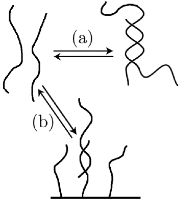
Figure 1: (a) Hybridization reaction in solution between partially complementary mRNA strands. (b) Hybridization reaction between mRNA strand from solution and substrate-based microarray DNA probe.

III.1 The sample

For the computation we considered a database containing $33,457$ human mRNA’s sequences downloaded from ftp.ncbi.nih.gov/refseq/H_sapiens/mRNA_Prot/, file human.rna.fna. These transcripts have an average length of several thousand nucleotides. However, in typical biochemical assays, as for instance in microarray experiments bald02 , the transcripts are present in shorter fragments of various lengths. We have chosen to divide the sequences into fragments of $48$ nucleotides, starting from the $5^{\prime}$ end of the transcript. The first fragment starts thus from nucleotide $n_{1}=1$ of the given transcript. The $m$-th fragment starts at nucleotide position $n_{m}=n_{m-1}+8$, i.e. with a shift of $8$ nucleotides from the previous one. This procedure avoids artifacts due to the exact location of the fragmentation point. For a transcript of length $L$ the fragmentation produces thus $L/8$ fragments, rounded down.

For the transcripts analyzed, the fragmentation produces in total $N=3,150,659$ different $48$-mers. To each of these an initial concentration $\overline{c}_{i}$ is assigned, such that fragments originating from the same transcript are given the same concentration. Input concentrations were obtained from DNA microarray data of Human mRNA in different tissues, using the outputs from the data analysis algorithm discussed in Ref. muld09 . Typical concentrations range from a few picomolars (pM) for low expressed genes, to nanomolar (nM) for the highly expressed genes.

The hybridization free energies $\Delta G_{ij}$, used in Eqs. (6) were computed using the nearest-neighbor model bloo00 , which assumes that the stability of the double helix depends on the identity and orientation of neighboring base pairs. The total free energy of a hybridizing strand is obtained as the sum of $10$ independent parameters accounting for hydrogen bonding and stacking interactions. In our computations we used the RNA/RNA parameters given in xia98 , at $1$M [Na+] and a temperature $T=55\celsius$.

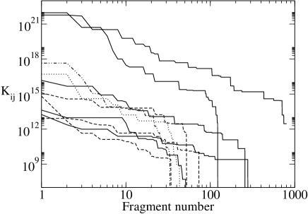
Figure 2: Plot of $K_{ij}$ for $10$ randomly selected fragments. The data are shown in decreasing order. It is seen in this figure that for each fragment, there are typically a few other fragments in the solution with which there is a significant interaction. Lists were generated containing all fragments which were complementary for at least 8 consecutive nucleotides. The number of ‘partners’ within a given free energy range is growing roughly exponentially, similar to what would be expected for randomly generated sequences. However, the Boltzmann factors $K_{ij}=e^{\beta\Delta G_{ij}}$ decrease faster, such that the highest few factors still dominate the sum $\sum_{j}c_{j}K_{ij}$ in the iterative scheme. Consequently, we can approximate this sum by truncating the list.

III.2 Efficient construction of interaction matrix

The iterative scheme presented above has a computational cost of order $N^{2}$: for each of the $N$ equations of (6) one has to compute the sum of $N$ terms. However, the analysis of the terms entering in the sum in the denominator of Eq. (6) shows that this sum is dominated by a few terms corresponding to the highest values of the hybridization free energy. Figure 2 shows a plot of the $K_{ij}$ for some randomly selected species $i$, as a function of $j$ ranked in decreasing order. The Boltzmann factors $K_{ij}=e^{\beta\Delta G_{ij}}$ decay rapidly as a function of $j$. As an approximation we kept only the first ten dominant terms for each $K_{ij}$, estimating that the typical error on the results is of a few percent. This improves the memory requirements of any implementation, and hence allows a much greater number of sequences to be present in our calculations.

To build up the matrix elements efficiently we generate a list of all possible sequences of length $l=8$ (this list has size $4^{l}$ and we refer to it as the primary list). We then run through all the mRNA sequences and generate an index vector which maps each position on a corresponding element of the primary list. This is an operation of order $N$. Having found two sequences $i$ and $j$ that are complementary for a stretch of length $l=8$, we can check if this complementarity can be extended to a longer stretch. This method is still of computational complexity of order $N^{2}$, however, with a small prefactor compared to a full complementarity matching. With the used method one ignores complementarity for stretches shorter than $l=8$ nucleotides, but these sequences would not be expected to cause significant hybridization anyways. The implementation can become very efficient by using binary operations: the four nucleotide types are encoded into two bits, complementarity can then be easily checked by a bitwise XOR operation.

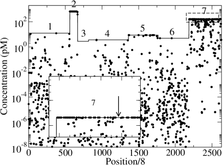
Figure 3: Initial concentrations ($\overline{c}_{i}$, solid line) and equilibrium single stranded concentration ($c^{*}_{i}$, circles) for seven selected transcripts. Fragments with a high total concentration are typically unaffected by hybridization in solution, but some of the fragments with a low total concentration get significantly depleted. Inset: zoom of the dashed zone around transcript $7$. The arrow shows a region where significant depletion has taken place.

III.3 Results

Once the initial concentrations $\overline{c}_{i}$ of the $N$ fragments are fixed, we repeatedly apply the map defined in Eq. (6). As proven before, the iterative procedure converges to a unique fixed point, representing the equilibrium concentration of fragments which are not hybridized.

In practice, the convergence criterion has been chosen such that the distance in concentration (using the distance $d(\vec{c},\vec{c}^{\prime})=\sum_{i}|c_{i}-c_{i}^{\prime}|/|c_{i}+c_{i}^{\prime}|$ for convenience) between two successive iterations is smaller than a given small value: $d(\vec{c}^{\,(k)},\vec{c}^{\,(k+1)})\leq\varepsilon$ with $\varepsilon=1$ Typically about $10^{2}$ iterations are sufficient to guarantee this level of accuracy.

Figure 3 shows a typical output of the computation for $7$ randomly chosen transcripts of varying lengths. The fragments are ordered as they are generated from the fragmentation procedure described above, thus the horizontal scale should be multiplied by a factor $8$ to have the length in nucleotides. The thin solid line corresponds to the total concentration $\overline{c}_{i}$ which, as mentioned before, is chosen to be constant for each transcript. For the transcripts shown in Fig. 3 the initial concentrations range from $2.8$ pM (for transcript $3$) to $670$ pM (for transcript $2$). The points denote the equilibrium concentration of single strands $c^{*}_{i}$, computed from the iterative algorithm. The figure shows different types of behaviors for the transcripts. Transcript $2$, which had the highest initial concentration, is weakly affected by hybridization with other fragments and most of the fragments have a free concentration very close to the initial one ${c}_{i}\approx\overline{c}_{i}$. Transcript $7$ is moderately affected by hybridization with other targets. A few of its fragments strongly hybridized with complementary partners in solution such that the concentration of free strands can drop of several orders of magnitude. The other transcripts, whose initial concentration was of few picomolars, are strongly affected and for almost all fragments, the free concentration is much lower than the initial concentration, ${c}_{i}\ll\overline{c}_{i}$.

As mRNA has typically a length of several thousands of nucleotides, there are many possible ways in which probes can be selected from it (most microarrays use as probes of 20-50 nucleotides). Probe design is a fundamental step in the realization of a DNA microarray. As an example, the results of Fig. 3(inset) suggest that a probe selected in the region marked by the arrow on transcript $7$ can significantly underestimate the true expression level of the transcript. As the transcript fragment strongly hybridizes in solution (reaction (a) of Fig. 1) a small concentration of single strand is available for hybridizing to the microarray surface (reaction (b) of Fig. 1). Based on these results, an additional important criterion for probe design should be the avoidance of strongly hybridizing transcriptomic regions.

Computations have been performed on different samples, differing by the values of the $\overline{c}_{i}^{\prime}s$, reflecting the different expression levels expected in different human tissues. The details of the computations will be presented elsewhere (F. Berger, M. G. A. van Dorp and E. Carlon, unpublished). As in the example above, we find in the transcriptome some regions strongly affected by mutual hybridization.

IV Convergence of the iterative procedure

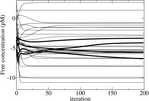
Figure 4: Convergence of $32$ species in the human transcriptome analysis. The horizontal axis is for the number of iterations, while the vertical axis shows the concentration for each of the $32$ probes at each iteration. Concentrations appear to be fairly stable at $200$ iterations, suggesting a fair degree of convergence. The four thicker lines correspond to four concentrations that display slow convergence.

In ths section we discuss the speed of convergence of the iterative algorithm for the specific example of mutual hybridizations in the human transcriptome and more in general for a generic hetero-dimerization network.

IV.1 Convergence for human transcriptome hybridization analysis

Figure 4 shows the concentrations $c_{i}^{(k)}$ of $32$ randomly selected species as a function of the iteration number $k$ for the reaction network of hybridizing mRNA fragments discussed in Section III. One notices that the convergence to the stationary value is attained for the majority of species after about $50$ iterations. However the speed of convergence varies for the different species, and in particular for three species in Fig. 4 convergence is much slower than average (thick lines). In all cases shown, after about $k\approx 200$ iterations $c_{i}^{(k)}$ has become mostly stationary.

The Banach theorem provides an estimate of the convergence rate given by $q$, as defined in Eq. (31). However this is not a very practical bound for convergence, as even in cases where just a few species bind very strongly to each other, we easily have $k_{\max}\overline{c}_{\max}\gg 1$. More realistic convergence rates can be obtained from the linear stability analysis around the fixed point.

IV.2 Linear stability analysis predictions for convergence

Given $N$ dimerizing species, we construct the matrix

$$\tilde{J}_{mn}\equiv-\frac{\partial T_{m}(\vec{c}^{\,*})}{\partial c_{n}}=\frac{K_{mn}\overline{c}_{m}}{(1+\sum_{j}K_{mj}c^{*}_{j})^{2}}=\frac{K_{mn}{c}^{*}_{m}}{1+\sum_{j}K_{mj}c^{*}_{j}}$$ (34)

where $\vec{T}(\vec{c})$ is the iterated map defined by Eq. (6) and $\vec{c}^{\,*}$ denotes the fixed point. Note that $\tilde{J}$ is obtained from the Jacobian matrix, by swapping the signs of all entries. The matrix $\tilde{J}$ is non-negative in the sense that for all its elements $\tilde{J}_{mn}\geq 0$. In the following we will use the notation $\vec{v}<\vec{w}$ if the inequality holds for all elements of the two vectors $\vec{v}$ and $\vec{w}$. For a non-negative matrix $J$, a common extension to the Perron-Frobenius theorem gant59 guarantees that there exists a (not necessarily unique) largest eigenvalue $r>0$ whose eigenvector $\vec{\phi}$ is non-negative, $\vec{\phi}\geq 0$. This eigenvector is known as the Perron-Frobenius vector. The largest eigenvalue $r$ determines the slowest convergence rate of the iterative scheme.

We have proven that the map $T$ is a contraction, hence necessarily $r<1$. We can however derive a stronger bound as follows. From $(\ref{jacobian})$ one derives

$$\left(\tilde{J}\vec{c}^{\,*}\right)_{m}=\sum_{n}\tilde{J}_{mn}{c}^{*}_{n}=\frac{\sum_{n}K_{mn}{c}^{*}_{n}}{1+\sum_{j}K_{mj}c^{*}_{j}}c_{m}^{*}\equiv\alpha_{m}c_{m}^{*}$$ (35)

Consider now $\tilde{J}^{T}$, the the transpose of $\tilde{J}$. The transpose has the same eigenvalues as $\tilde{J}$, but a different eigenvector. The Perron-Frobenius theorem applies also to $\tilde{J}^{T}$ for which $\tilde{J}^{T}\vec{\phi}{\,{}^{\prime}}=r\vec{\phi}{\,{}^{\prime}}$ and $\vec{\phi}{\,{}^{\prime}}\geq 0$. One has

$$r\vec{\phi}{\,{}^{\prime}}\cdot\vec{c}^{\,*}=\tilde{J}^{T}\vec{\phi}{\,{}^{\prime}}\cdot\vec{c}^{\,*}=\vec{\phi}{\,{}^{\prime}}\cdot\tilde{J}\vec{c}^{\,*}$$ (36)

where the dot indicates the scalar product.

Working out this scalar product and using Eq. (35) one finds

$$r\sum_{m}\phi^{\prime}_{m}{c^{*}_{m}}=\sum_{m}\phi^{\prime}_{m}\alpha_{m}{c^{*}_{m}}\leq\max_{n}\{\alpha_{n}\}\sum_{m}\phi^{\prime}_{m}{c^{*}_{m}}$$ (37)

where we have used the fact that $\phi^{\prime}_{m}\geq 0$ and $c^{*}_{m}\geq 0$ Equation (37) shows that

$$r\leq\max_{m}\frac{\sum_{j}K_{mj}{c}^{*}_{j}}{1+\sum_{j}K_{mj}c^{*}_{j}}<1.$$ (38)

For most networks, especially those where most values $K_{mn}$ are small and only a few ones are very large, this is a better bound to the convergence rate compared to that guaranteed by Banach’s theorem (Eq. (31)) as:

$$\max_{m}\frac{\sum_{j}K_{mj}{c}^{*}_{j}}{1+\sum_{j}K_{mj}c^{*}_{j}}=\frac{1}{1+\frac{1}{\max_{m}\sum_{j}K_{mj}{c}^{*}_{j}}}<q$$ (39)

where $q$ is the Lipschitz constant given by Eq. (31).

The largest eigenvalue of the Jacobian matrix provides the slowest rate of convergence. The example of Fig. 4 shows that the convergence rate may differ for different species. We provide here some simple insights on possible origins of the slow convergence.

Consider first reaction networks for which the dimerization process is very weak, so that the equilibrium concentrations $c_{m}^{*}$ differ only weakly from the total concentration $\overline{c}_{m}$. In this case $K_{mn}c^{*}_{n}\ll 1$, hence Eq. (38) implies fast convergence.

More interesting is the case of strongly interacting networks, where slow relaxation to equilibrium is expected. To illustrate this, consider two strongly interacting species for which dimerization is so strong that interaction with the rest of the network can be neglected in first approximation. This two species system is described by the equations

$$c_{1}=\frac{\overline{c}_{1}}{1+Kc_{2}}$$ (40)

$$c_{2}=\frac{\overline{c}_{2}}{1+Kc_{1}}$$ (41)

where for simplicity we discard the possibility of self-dimerization and $K=K_{12}=K_{21}$. The diagonal elements of the Jacobian vanish ($\tilde{J}_{11}=\tilde{J}_{22}=0$), therefore the rate of convergence (eigenvalues of $\tilde{J}$) is given by

$$\lambda=\pm\sqrt{\tilde{J}_{12}\tilde{J}_{21}}$$ (42)

We consider now two different cases: (1) $\overline{c}_{1}=\overline{c}_{2}=\overline{c}$ and $K\overline{c}\gg 1$ and (2) $\overline{c}_{1}\gg\overline{c}_{2}$ and $K\overline{c}_{2}\gg 1$.

The case (1) corresponds to the two species having the same initial concentration and strongly dimerizing to each other. In equilibrium $c^{*}_{1}=c^{*}_{2}\ll\overline{c}$. Some simple algebra shows that the eigenvalues of the Jacobian become

$$\lambda=\pm 1+{\cal O}\left(\frac{1}{\sqrt{K\overline{c}}}\right)$$ (43)

which implies a very slow convergence, as $|\lambda|$ is close to $1$. In the case (2) one finds

$$\lambda=\pm\sqrt{\frac{\overline{c}_{2}}{\overline{c}_{1}}}$$ (44)

which is small when $\overline{c}_{1}\gg\overline{c}_{2}$. This implies very fast convergence.

If this type of problems would be encountered in large networks, we suggest to solve them by computing analytically the equilibrium values for the subnetwork containing only these two species. Putting the resulting equilibrium concentrations as initial concentrations in the full network, the iterative scheme should converge fast. Finally, we remark that problematic cases can easily be detected by checking whether $\overline{c}_{1}\approx\overline{c}_{2}$. If this is not the case, convergence will necessarily be fast.

V Conclusions

We have described a novel algorithm to efficiently compute the equilibrium concentrations for a class of chemical reaction networks. The core part of our algorithm is an iterative procedure, which we have shown to converge to the unique stable point of the system. Furthermore, we have analysed the convergence properties to conclude that convergence is typically fast, except in certain problematic cases. These problems turn out to be easy to detect, and the solution to these problems by analytically solving subnetworks could eventually be implemented.

The inspiration for considering this problem can be traced back to the analysis of physical models describing experiments with DNA microarrays. Consequently, we have implemented our algorithm specifically to test whether it can be used to find the equilibrium concentrations for a system of this size, where of the order of $10^{6}$ different RNA fragments form a large reaction network. We found that convergence was quick, on the order of at most a few hundred iterations, and that the full computation took only a few minutes on a mainstream desktop PC.

In the present work we have restricted our analysis to hetero-dimerization networks with mass action kinetics. It would be very interesting to expand these iterative algorithms to a wider class of chemical reaction networks, particularly for the case of genetic regulatory networks dejo02 . One factor limiting the study of these networks is that often the values of reaction rates are not known apart for very few well studied cases dejo02 . The steady state analysis has to be repeated for various input rates, therefore it is very important to have fast algorithms, which could perform this analysis efficiently.

References

- (1) M. Feinberg, Chem. Eng. Sci. 42, 2229 (1987).
- (2) H. de Jong, J. Comput. Biol. 9, 67 (2002).
- (3) Z. P. Gerdtzen, P. Daoutidis, and W.-S. Hu, Metab. Eng. 6, 140 (2004)
- (4) C. Conradi, J. Saez-Rodriguez, E. D. Gilles, and J. Raisch, IEE Proc. Syst. Biol. 152, 243 (2005)
- (5) U. Alon, Introduction to Systems Biology: Design Principles of Biological Circuits (Chapman & Hall, 2006)
- (6) I. Martínez-Forero, A. Peláez-López, and P. Villoslada, PLoS One 5, e10823 (2010).
- (7) G. Shinar and M. Feinberg, Science 327, 1389 (2010)
- (8) D. Zwicker, D. K. Lubensky, and P. R. ten Wolde, Proc Natl Acad Sci U S A 107, 22540 (2010)
- (9) C. Pantea and G. Craciun, in Circuits and Systems (ISCAS), Proceedings of 2010 IEEE International Symposium on (2010) pp. 549 –552
- (10) M. P. Millan, A. Dickenstein, A. Shiu, and C. Conradi, arXiv1102.1590(2011), 1102.1590
- (11) E. Carlon and T. Heim, Physica A 362, 433 (2006).
- (12) H. Binder, J. Phys.: Condens. Matt. 18, S491 (2006).
- (13) C. J. Burden, Y. Pittelkow, and S. R. Wilson, J. Phys.: Condens. Matter 18, 5545 (2006).
- (14) A. Halperin, A. Buhot, and E. B. Zhulina, J. Phys. Cond. Matt. 18, S463 (2006)
- (15) A. Granas and J. Dugundji, Fixed Point Theory (Springer-Verlag, New York, 2003)
- (16) P. Baldi and G. W. Hatfield, DNA microarrays and gene expression: from experiments to data analysis and modeling (Cambridge University Press, 2002)
- (17) M. T. Horne, D. J. Fish, and A. S. Benight, Biophys J 91, 4133 (2006).
- (18) G. C. W. M. Mulders, G. T. Barkema, and E. Carlon, BMC Bioinformatics 10, 64 (2009).
- (19) V. A. Bloomfield, D. M. Crothers, and I. Tinoco, Jr., Nucleic Acids Structures, Properties and Functions (University Science Books, Mill Valley, 2000)
- (20) T. Xia, J. SantaLucia, M. E. Burkard, R. Kierzek, S. J. Schroeder, X. Jiao, C. Cox, and D. H. Turner, Biochemistry 37, 14719 (1998).
- (21) F. R. Gantmacher, The theory of matrices, Volume 2 (Chelsea Publishing Company, 1959)