Line tension of branching junctions of bilayer membranes

Abstract

Branching of bilayer membranes appear in the inverted hexagonal phase as well as in metastable states of the lamellar phase such as membrane fusion intermediates. A method for estimating the line tension of the branching junction is proposed for molecular simulations. The line tension is calculated from the pressure tensor of equiangularly branched membranes. The simulation results agree very well with the theoretical prediction of Hamm and Kozlov’s tilt model. The transition between the lamellar and inverted hexagonal phases is also investigated using the tilt model.

I Introduction

Amphiphilic molecules, such as lipids and detergents, self-assemble into various structures: spherical or cylindrical micelles; lamella; and hexagonal, cubic, and sponge structures Israelachvili (2011); Lipowsky and Sackmann (1995); Gruner et al. (1985); Gruner (1989). The bilayer membrane in the lamellar phase is the basic structure of the plasma membrane and the intracellular compartments of living cells. It is known that biological membranes contain a substantial amount of lipids that can adopt the inverted hexagonal $H_{II}$ phase upon isolation Verkleij (1984); Epand (1998); Hafez and Cullis (2001). Thus, it has been speculated that non-bilayer structures play some roles in biological functions such as membrane fusion and other membrane contact phenomena such as tight junctions.

Several mechanisms of membrane fusion have been proposed Jahn and Grubmüller (2002); Chernomordik and Kozlov (2008); Nikolaus et al. (2011); Markvoort and Marrink (2011); Müller and Schick (2011). Among these, the stalk model is widely accepted. According to this model, two vesicles form a metastable structure, the stalk intermediate, where the outer monolayers (leaflets) are connected with a cylindrical (stalk) structure. Next, radial expansion of the stalk Chernomordik and Kozlov (2008); Siegel (1993) or a pore opening on the side of the stalk Müller and Schick (2011); Noguchi and Takasu (2001a) leads to either complete fusion or the formation of a hemifusion diaphragm (HD) intermediate. In the HD, the inner monolayers of two vesicles form a bilayer membrane, which connects with two bilayer membranes of the vesicles via a branching junction. Many experiments support that fusion proceeds through a metastable intermediate state, which is considered to be the stalk or HD intermediate. Recently, molecular simulations of membrane fusion and fission have been reported by several groups Markvoort and Marrink (2011); Müller and Schick (2011); Noguchi and Takasu (2001a, 2002a, 2002b); Noguchi (2002); Müller et al. (2002); Marrink and Mark (2003); Li and Liu (2005); Smeijers et al. (2006); Knecht and Marrink (2007); Gao et al. (2008). In most of these simulations, the stalk intermediate is formed first. However, the pathway of the stalk to complete fusion is not unique and is dependent on the simulation conditions. Thus far, it has not been determined which membrane properties and external conditions determine the fusion pathways. It is important to estimate the free energy of each fusion intermediate to understand the fusion pathways.

Since the transition between lamellar and $H_{II}$ phases requires the same type of topological changes as membrane fusion, it is considered to proceed through similar pathways Siegel (1993); Li and Schick (2000). Recently, the phase of a hexagonally ordered stalk structure has been observed between lamellar and $H_{II}$ phases Yang and Huang (2002). Here, we consider the $H_{II}$ structure with a long cell length. The bilayer membranes are connected with hexagonally arranged branching junctions. When the branching junctions of bilayers are isolated, i.e., sufficiently far from other junctions, the free energy of a junction is proportional to the junction length. Thus, it can be estimated as a line tension. In this paper, we propose a method for estimating this line tension for molecular simulations. This tension quantifies the stability of the HD fusion intermediate.

To simulate lipid membranes on long and large scales, various coarse-grained molecular models have been proposed (see review articles Müller et al. (2006); Venturoli et al. (2006); Noguchi (2009); Marrink et al. (2009)). Recently, the bottom-up approaches have been intensively investigated to construct coarse-grained molecular models, in which potential parameters are tuned from atomistic simulations Marrink et al. (2004); Izvekov and Voth (2005); Arkhipov et al. (2008); Shinoda et al. (2008); Wang and Deserno (2010). We, on the other hand, choose an opposite top-down approach to construct the coarse-grained molecular models, in which potentials are based on the continuum theory. Here, we employ a spin lipid molecular model Noguchi (2011a), which is one of the solvent-free molecular lipid models Noguchi (2009). In this model, the membrane properties (bending rigidity, line tension of membrane edge, area compression modulus, lateral diffusion coefficient, and flip-flop rate) can be varied over wide ranges.

In Sec. II, the simulation method and the membrane properties of the simulation model are described. In Secs. III and IV, the line tension is estimated by the simulation and the tilt model, respectively. The line tension is calculated from the pressure tensor of hexagonally arranged membrane branches. Previously, the line tension of the membrane edge has been estimated from the pressure tensor of a membrane strip Tolpekina et al. (2004); Wang and Deserno (2010); Noguchi (2011a). For branching junctions the membrane can hold finite surface tension, unlike the strip, hence, the membrane area should be carefully treated. The tilt model proposed by Hamm and Kozlov Hamm and Kozlov (1998, 2000) reproduces the simulation results very well. In Sec. V, the rupture dynamics of the branches and the HD intermediates of the vesicles are shown. Finally, a summary is given in Sec. VI.

II Simulation Model and Method

II.1 Membrane Model

A spin lipid molecular model Noguchi (2011a) is used to simulate bilayer membranes. Each ($i$-th) molecule has a spherical particle with an orientation vector ${\bf u}_{i}$, which represents the direction from the hydrophobic to the hydrophilic part ($|{\bf u}_{i}|=1$). There are two points of interaction in the molecule: the center of a sphere ${\bf r}^{\rm s}_{i}$ and a hydrophilic point ${\bf r}^{\rm e}_{i}={\bf r}^{\rm s}_{i}+{\bf u}_{i}\sigma$. The molecules interact with each other via the potential,

$$\frac{U}{k_{\rm B}T} =\ \ \hskip 28.45274pt\sum_{i<j}U_{\rm{rep}}(r_{ij}^{\rm s})+\varepsilon\sum_{i}U_{\rm{att}}(\rho_{i})$$

$$\ \ + \ \ \frac{k_{\rm{tilt}}}{2}\sum_{i<j}\bigg{[}({\bf u}_{i}\cdot\hat{\bf r}^{\rm s}_{ij})^{2}+({\bf u}_{j}\cdot\hat{\bf r}^{\rm s}_{ij})^{2}\bigg{]}w_{\rm{cv}}(r^{\rm e}_{ij})$$

$$\ \ + \frac{k_{\rm{bend}}}{2}\sum_{i<j}\bigg{(}{\bf u}_{i}-{\bf u}_{j}-C_{\rm{bd}}\hat{\bf r}^{\rm s}_{ij}\bigg{)}^{2}w_{\rm{cv}}(r^{\rm e}_{ij}),$$

where ${\bf r}_{ij}={\bf r}_{i}-{\bf r}_{j}$, $r_{ij}=|{\bf r}_{ij}|$, $\hat{\bf r}_{ij}={\bf r}_{ij}/r_{ij}$, and $k_{\rm B}T$ is the thermal energy. The molecules have an excluded volume with a diameter $\sigma$ via the repulsive potential, $U_{\rm{rep}}(r)=\exp[-20(r/\sigma-1)]$, with a cutoff at $r=2.4\sigma$.

The second term in Eq. (II.1) represents the attractive interaction between the molecules. An attractive multibody potential $U_{\rm{att}}(\rho_{i})$ is employed to mimic the “hydrophobic” interaction. This potential allows the formation of the fluid membrane over wide parameter ranges. Similar potentials have been applied in other membrane models Noguchi and Takasu (2001b); Noguchi and Gompper (2006); Farago and Grønbech-Jensen (2009) and a coarse-grained protein model Takada et al. (1999). The potential $U_{\rm{att}}(\rho_{i})$ is given by

$$U_{\rm{att}}(\rho_{i})=0.25\ln[1+\exp\{-4(\rho_{i}-\rho^{*})\}]-C,$$ (2)

with $C=0.25\ln\{1+\exp(4\rho^{*})\}$. The local particle density $\rho_{i}$ is approximately the number of particles ${\bf r}^{\rm s}_{i}$ in the sphere with radius $r_{\rm{att}}$.

$$\rho_{i}=\sum_{j\neq i}f_{\rm{cut}}(r^{\rm s}_{ij}),$$ (3)

where $f_{\rm{cut}}(r)$ is a $C^{\infty}$ cutoff function,

$$f_{\rm{cut}}(r)=\left\{\begin{array}[]{ll}\exp\{A(1+\frac{1}{(r/r_{\rm{cut}})^{n}-1})\}&(r<r_{\rm{cut}})\\ 0&(r\geq r_{\rm{cut}})\end{array}\right.$$ (4)

with $n=6$, $A=\ln(2)\{(r_{\rm{cut}}/r_{\rm{att}})^{n}-1\}$, $r_{\rm{att}}=1.9\sigma$ $(f_{\rm{cut}}(r_{\rm{att}})=0.5)$, and the cutoff radius $r_{\rm{cut}}=2.4\sigma$. The density $\rho^{*}$ in $U_{\rm{att}}(\rho_{i})$ is the characteristic density. For $\rho_{i}<\rho^{*}-1$, $U_{\rm{att}}(\rho_{i})$ acts as a pairwise attractive potential while it approaches a constant value for $\rho_{i}>\rho^{*}+1$.

The third and fourth terms in Eq. (II.1) are discretized versions of the tilt and bending potentials of the tilt model Hamm and Kozlov (1998, 2000), respectively. A smoothly truncated Gaussian function Noguchi and Gompper (2006) is employed as the weight function

$$w_{\rm{cv}}(r)=\left\{\begin{array}[]{ll}\exp(\frac{(r/r_{\rm{ga}})^{2}}{(r/r_{\rm{cc}})^{n}-1})&(r<r_{\rm{cc}})\\ 0&(r\geq r_{\rm{cc}})\end{array}\right.$$ (5)

with $n=4$, $r_{\rm{ga}}=1.5\sigma$, and $r_{\rm{cc}}=3\sigma$. All orders of derivatives of $f_{\rm{cut}}(r)$ and $w_{\rm{mls}}(r)$ are continuous at the cutoff radii. The weight is a function of $r^{\rm e}_{ij}$ to avoid the interaction between the molecules in the opposite monolayers of the bilayer. If $r^{\rm s}_{ij}$ is employed instead, a single-layer membrane is formed Shiba and Noguchi (2011).

II.2 Simulation Method

The bilayer membrane is simulated in the $NVT$ ensemble (constant number of molecules $N$, volume $V$, and temperature $T$) and Brownian dynamics (molecular dynamics with Langevin thermostat) is employed. The motion of the center of the mass ${\bf r}^{\rm G}_{i}=({\bf r}^{\rm s}_{i}+{\bf r}^{\rm e}_{i})/2$ and the orientation ${\bf u}_{i}$ are given by underdamped Langevin equations:

$$\frac{d{\bf r}^{\rm G}_{i}}{dt} = {\bf v}^{\rm G}_{i},\ \ \frac{d{\bf u}_{i}}{dt}={\bm{\omega}}_{i},$$ (6)

$$m\frac{d{\bf v}^{\rm G}_{i}}{dt} = -\zeta_{\rm G}{\bf v}^{\rm G}_{i}+{\bf g}^{\rm G}_{i}(t)+{\bf f}^{\rm G}_{i},$$ (7)

$$I\frac{d{\bm{\omega}}_{i}}{dt} = -\zeta_{\rm r}{\bm{\omega}}_{i}+({\bf g}^{\rm r}_{i}(t)+{\bf f}^{\rm r}_{i})^{\perp}+\lambda_{\rm L}{\bf u}_{i},$$ (8)

where $m$ and $I$ are the mass and the moment of inertia of the molecule, respectively. The forces are given by ${\bf f}^{\rm G}_{i}=-\partial U/\partial{\bf r}^{\rm G}_{i}$ and ${\bf f}^{\rm r}_{i}=-\partial U/\partial{\bf u}_{i}$ with the perpendicular component ${\bf a}^{\perp}={\bf a}-({\bf a}\cdot{\bf u}_{i}){\bf u}_{i}$ and a Lagrange multiplier $\lambda_{\rm L}$ to keep ${\bf u}_{i}^{2}=1$. According to the fluctuation-dissipation theorem, the friction coefficients $\zeta_{\rm G}$ and $\zeta_{\rm r}$ and the Gaussian white noises ${\bf g}^{\rm G}_{i}(t)$ and ${\bf g}^{\rm r}_{i}(t)$ obey the following relations: the average $\langle g^{\beta_{1}}_{i,\alpha_{1}}(t)\rangle=0$ and the variance $\langle g^{\beta_{1}}_{i,\alpha_{1}}(t_{1})g^{\beta_{2}}_{j,\alpha_{2}}(t_{2})\rangle=2k_{\rm B}T\zeta_{\beta_{1}}\delta_{ij}\delta_{\alpha_{1}\alpha_{2}}\delta_{\beta_{1}\beta_{2}}\delta(t_{1}-t_{2})$, where $\alpha_{1},\alpha_{2}\in\{x,y,z\}$ and $\beta_{1},\beta_{2}\in\{{\rm G,r}\}$. The Langevin equations are integrated by the leapfrog algorithm Allen and Tildesley (1987); Noguchi (2011a).

The results are displayed with a length unit of $\sigma$, an energy unit of $k_{\rm B}T$, and a time unit of $\tau_{0}=\zeta_{\rm G}\sigma^{2}/k_{\rm B}T$. $m=\zeta_{\rm G}\tau_{0}$, $I=\zeta_{\rm r}\tau_{0}$, $\zeta_{\rm r}=\zeta_{\rm G}\sigma^{2}$, $\Delta t=0.005\tau_{0}$, and $\rho^{*}=14$ are used. The error bars of the data are estimated from the standard deviations of three or six independent runs.

II.3 Membrane Properties

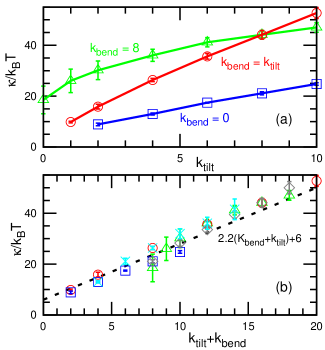
Figure 1: Bending rigidity $\kappa$ dependence on (a) $k_{\rm{tilt}}$ and (b) $k_{\rm{tilt}}+k_{\rm{bend}}$ for $\varepsilon=2$ and $C_{\rm{bd}}=0$. The lines with squares, circles, and triangles represent data for $k_{\rm{bend}}=0$, $k_{\rm{bend}}=k_{\rm{tilt}}$, and $k_{\rm{bend}}=8$, respectively. The crosses and diamonds represent data for $k_{\rm{tilt}}=4$ and $8$, respectively, for several values of $k_{\rm{bend}}$. The dashed line shows $\kappa/k_{\rm B}T=2.2(k_{\rm{tilt}}+k_{\rm{bend}})+6$.

The potential-parameter dependence of the membrane properties (bending rigidity $\kappa$, line tension $\Gamma$ of membrane edge, area compression modulus, lateral diffusion coefficient, and flip-flop rate) are investigated in detail in our previous paper Noguchi (2011a). In this model, these properties can be varied over wide ranges. The line tension $\Gamma$ of the membrane edge can be controlled by varying $\varepsilon$ and $C_{\rm{bd}}$. The membrane has a wide range of fluid phases, and the fluid-gel transition point can be controlled by $\rho^{*}$. The area compression modulus $K_{\rm A}$ can be varied by $k_{\rm{tilt}}$. The flip-flop rate can be varied by $k_{\rm{tilt}}$ and $k_{\rm{bend}}$.

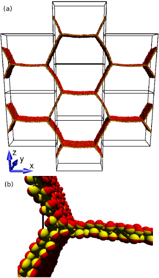
Figure 2: Snapshot of the bilayer membranes with hexagonally arranged branches for $N=3072$, $L_{x}=\sqrt{3}L_{z}/2=56\sigma$, $L_{y}=16.94\sigma$, $\varepsilon=2$, $k_{\rm{bend}}=8$, $k_{\rm{tilt}}=8$, and $C_{\rm{bd}}=0$. (a) Periodic images. (b) Magnified snapshot of the branching junction. The red and yellow himispheres represent the hydrophilic and hydrophobic parts of the molecules, respectively.

The bending rigidity $\kappa$ is linearly dependent on $k_{\rm{tilt}}$ and $k_{\rm{bend}}$. The spectra of undulation modes $\langle|h(q)|^{2}\rangle=k_{\rm B}T/\kappa q^{4}$ are widely used to estimate $\kappa$ for tensionless planar membranes. In Ref. Noguchi (2011a), we use a least-squares fit to $1/\langle|h(q)|^{2}\rangle=\kappa q^{4}/k_{\rm B}T$ for low frequency modes $q<q_{\rm{cut}}$ with $(q_{\rm{cut}}/\pi)^{2}=0.015$. More recently, we have found that the extrapolation to $q_{\rm{cut}}\to 0$ yields a better $\kappa$ estimation Shiba and Noguchi (2011). Re-estimated values of $\kappa$ are shown in Fig. 1 for the tensionless membrane using this extrapolation method. Slightly higher values are obtained and the slope $2$ in Ref. Noguchi (2011a) becomes $2.2$ as $\kappa/k_{\rm B}T=2.2(k_{\rm{tilt}}+k_{\rm{bend}})+6$ for $\varepsilon=2$ [see Fig. 1(b)].

The bending elasticity generated by the bending and tilt potentials can be derived from the continuum theory Safran (1994); Helfrich (1973) as discussed in Refs. Noguchi (2011a); Shiba and Noguchi (2011). When the orientation vectors ${\bf u}_{i}$ are equal to the normal vectors ${\bf n}$ of the membrane without tilt deformation, the bending and tilt energies of the monolayer membrane are given by

$$U_{\rm{cv}} = \int dA\ \frac{\kappa^{*}_{\rm{bend}}+\kappa^{*}_{\rm{tilt}}}{2}(C_{1}+C_{2}-C_{0})^{2}$$ (9)

$$\hskip 25.6073pt-(\kappa^{*}_{\rm{bend}}+\kappa^{*}_{\rm{tilt}})C_{1}C_{2}$$

in the continuum limit, where $C_{1}$ and $C_{2}$ are the two principal curvatures of the monolayer membrane. The bending rigidity and the saddle-splay modulus of the monolayer are given by $\kappa_{\rm{mo}}=\kappa^{*}_{\rm{bend}}+\kappa^{*}_{\rm{tilt}}$ and $\bar{\kappa}_{\rm{mo}}=-\kappa$, respectively. The spontaneous curvature is given by $C_{0}=\{\kappa^{*}_{\rm{bend}}/(\kappa^{*}_{\rm{bend}}+\kappa^{*}_{\rm{tilt}})\}C_{\rm{bd}}/\bar{r}_{\rm{nb}}$, where $\bar{r}_{\rm{nb}}$ is the nearest-neighbor distance. By assuming a hexagonal packing of the molecules, the bending rigidities generated by the bending and tilt potentials are estimated as $\kappa^{*}_{\rm{bend}}/k_{\rm B}T=\sqrt{3}k_{\rm{bend}}w_{\rm{cv}}(\bar{r}_{\rm{nb}})$ and $\kappa^{*}_{\rm{tilt}}/k_{\rm B}T=\sqrt{3}k_{\rm{tilt}}w_{\rm{cv}}(\bar{r}_{\rm{nb}})/2$, respectively. Thus, the bending rigidity $\kappa$ of the bilayer membrane is estimated as $\kappa=2\kappa_{\rm{mo}}\simeq(2.1k_{\rm{bend}}+1.1k_{\rm{tilt}})k_{\rm B}T$ from $\bar{r}_{\rm{nb}}\simeq 1.05\sigma$ and $w_{\rm{cv}}(1.05\sigma)=0.61$. This estimation of $\kappa$ shows quantitative agreement with the simulation results for $k_{\rm{bend}}$, while the prefactor of $k_{\rm{tilt}}$ is half that of the numerical estimation. Deviation from a hexagonal lattice and tilt deformation likely change the prefactor of $k_{\rm{tilt}}$. Using $\kappa^{**}_{\rm{tilt}}=2\kappa^{*}_{\rm{tilt}}$, the spontaneous curvature $C_{0}\simeq\{k_{\rm{bend}}/(k_{\rm{bend}}+k_{\rm{tilt}})\}C_{\rm{bd}}/\sigma$ is obtained, which agrees well with $C_{0}$ calculated from a membrane tube and strip Shiba and Noguchi (2011). Positive spontaneous curvature indicates that the hydrophilic head is larger than the hydrophobic tail of amphiphilic molecules.

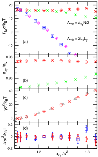
Figure 3: Dependence of the junction line tension $\Gamma_{\rm{br}}$ and surface tension $\gamma$ on the membrane area $a_{xy}$ per molecule for $\varepsilon=8$, $k_{\rm{bend}}=8$, $k_{\rm{tilt}}=8$, and $C_{\rm{bd}}=0$. (a) The line tension $\Gamma_{\rm{br}}$ calculated from Eq. (12) with $A_{\rm{mb}}=a_{xy}N/2$ ($\circ,\times$) and $A_{\rm{mb}}=2_{x}Ly$ ($\Box,\diamond$). The symbols ($\times,\diamond$) and ($\circ,\Box$) represent data for $N=1536$ and $N=3072$, respectively. (b) The molecular area $a_{xy}$ for the bilayer in the middle of the simulation box is compared with the geometrically estimated area $a_{\rm L}=4L_{x}L_{y}/N$ for $N=1536$ ($\times$) and $N=3072$ ($\circ$). (c) The surface tension $\gamma$ calculated from the branched membranes ($\circ$) for $N=3072$ and the previous simulation of the planar bilayer membrane ($\triangle$) for $N=512$. (d) The differences in the values of $\gamma$ estimated from the three methods for $N=3072$. The circles ($\circ$) and squares ($\Box$) represent $\gamma_{z}-\gamma_{x}$ and $\gamma_{\rm{mid}}-\gamma_{x}$, respectively. The tensions $\gamma_{x}$ and $\gamma_{z}$ are calculated from the pressure tensors $P_{xx}$ and $P_{zz}$, respectively. The tension $\gamma_{\rm{mid}}$ is calculated from the middle bilayer.

III Measurement of line tension of branching junctions

To measure the stress of branched membranes, we consider hexagonally arranged branches (see Fig. 2). These have an inverted hexagonal structure with a long cell length. Three membranes equiangularly connect with each other at the branching junction. The periodic boundary along the $x$ direction is shifted as shown in Fig. 2(a). Normal periodic boundary conditions are employed in the $y$ and $z$ directions. Thus, the periodic images are given by $(x_{i}+n_{x}L_{x},y_{i}+n_{y}L_{y},z_{i}+n_{z}L_{z}+n_{x}L_{z}/2)=(x_{i},y_{i},z_{i})$, where $n_{x}$, $n_{y}$, and $n_{z}$ are arbitrary integers for a simulation box with side lengths $L_{x}$, $L_{y}$, and $L_{z}$. Length $L_{y}$ is varied to change the membrane area and surface tension. The other side lengths are fixed as $L_{x}=\sqrt{3}L_{z}/2=28\sigma$ and $56\sigma$ for $N=1536$ and $3072$, respectively. When the membrane thickness is neglected, the total membrane area in the simulation box is $A_{\rm L}=2L_{x}L_{y}$, since the area of one membrane is $2L_{x}L_{y}/3$ and three membranes exist in the box. The length of one branching junction is $L_{y}$, and two junctions are in the box. The origin $(x,y,z)=(0,0,0)$ is set at the center of the simulation box and is kept at the center of the horizontal membrane.

The line tension of the branching junction can be calculated from the diagonal components of the pressure tensor

$$P_{\alpha\alpha}=\big{(}Nk_{\rm B}T-\sum_{i}\alpha_{ij}\frac{\partial U}{\partial{\alpha}_{ij}}\big{)}/V,$$ (10)

where $\alpha\in\{x,y,z\}$ and $V=L_{x}L_{y}L_{z}$. The stresses should be generated by the line tension $\Gamma_{\rm{br}}$ of the branching junction, the surface tension $\gamma$, and the bulk pressure $P_{\rm{bulk}}$.

$$P_{xx}V = P_{\rm{bulk}}V-\gamma L_{x}L_{y},$$ (11)

$$P_{yy}V = P_{\rm{bulk}}V-\gamma A_{\rm{mb}}-2\Gamma_{\rm{br}}L_{y},$$ (12)

$$P_{zz}V = P_{\rm{bulk}}V-\frac{\sqrt{3}}{2}\gamma L_{y}L_{z}.$$ (13)

In the membranes with an angle of $\pm\pi/3$ to the $xy$ plane, the surface tension yields stresses $\gamma/2$ and $(\sqrt{3}/2)\gamma$ in the $x$ and $z$ directions, respectively. Since the membranes can be moved in the $x$ and $z$ directions, these stresses are balanced i.e. $P_{xx}=P_{zz}$. Indeed, Eqs. (11) and (13) give the same value. Since all membranes are parallel to the $y$ direction, the total membrane area $A_{\rm{mb}}$ in the simulation box is used in Eq. (12). Since the critical micelle concentration (CMC) is low and no isolated molecules appear, the bulk pressure $P_{\rm{bulk}}$ is negligibly small in our solvent-free simulations.

To estimate the line tension $\Gamma_{\rm{br}}$, the surface tension $\gamma$ has to be calculated first. In the simulations, $\gamma$ can be estimated from $P_{xx}$ or $P_{zz}$. We called them $\gamma_{x}$ and $\gamma_{z}$, respectively. We also calculated $\gamma$ from the middle of the bilayer membrane which is parallel to the $xy$ plane using the definition for the planar interface, $\gamma_{\rm{mid}}=\langle P_{zz}-(P_{xx}+P_{yy})/2\rangle L_{z}$ for $-L_{x}/12<x<L_{x}/12$. The estimated values of $\gamma$ from these three methods agree very well [see Fig. 3(d)]. We use the average value $\gamma=(\gamma_{x}+\gamma_{z})/2$ as the surface tension to reduce statistical errors. Here, we only consider membranes with small or positive surface tensions, i.e., exclude the buckled membranes under lateral compression, since the surface tension becomes anisotropic in buckled membranes Noguchi (2011b).

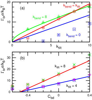
Figure 4: Dependence of the line tension $\Gamma_{\rm{br}}$ of the branching junction on (a) $k_{\rm{tilt}}$ and (b) $C_{\rm{bd}}$. (a) The squares, circles, and triangles represent data for $k_{\rm{bend}}=0$, $k_{\rm{bend}}=k_{\rm{tilt}}$, and $k_{\rm{bend}}=8$, respectively, at $\varepsilon=2$ and $C_{\rm{bd}}=0$. (b) The symbols ($\circ$, $\Box$) and ($\times,\diamond$) represent data for $\varepsilon=2$ and $8$, respectively, at $k_{\rm{bend}}=k_{\rm{tilt}}=4$ or $8$. The solid lines in (a) and (b) are obtained from Eq. (22).

Next, we consider the membrane area. The projected area $a_{xy}$ per molecule is calculated from the middle of the membrane at $-L_{x}/12<x<L_{x}/12$ as $a_{xy}=(L_{x}L_{y}/6)/(N_{\rm{mid}}/2)$ where $N_{\rm{mid}}$ is the number of the molecules at $-L_{x}/12<x<L_{x}/12$. The $a_{xy}$ dependence of $\gamma$ calculated from branched membranes agrees with that obtained from planar membranes [see Fig. 3(c)]. This area $a_{xy}$ is slightly smaller than the area $a_{\rm L}=2L_{x}L_{y}/(N/2)$ calculated from the geometry. The decreases are $4$% and $2$% for $N=1536$ and $3072$, respectively, as shown in Fig. 3(b). These deviations are caused by the membrane thickness. In Fig. 5, the length of the membrane surface is shorter than the center line of the membrane. Thus, the monolayer (leaflet) area of the bilayer membrane becomes smaller than $a_{\rm L}$.

Finally, the line tension $\Gamma_{\rm{br}}$ of the branching junction is estimated from the pressure tensor and $a_{xy}$,

$$\Gamma_{\rm{br}}=\Big{\{}(P_{xx}+P_{zz})\frac{a_{xy}}{a_{\rm L}}-P_{yy}\Big{\}}\frac{V}{2L_{y}}.$$ (14)

In explicit solvent simulations ($P_{\rm{bulk}}\neq 0$), $\gamma$ or $P_{\rm{bulk}}$ should be calculated from a local region in the simulation box. When $\gamma_{\rm{mid}}$ is used, the line tension is given by

$$\Gamma_{\rm{br}}=\Bigg{\{}\Big{(}\frac{P_{xx}+P_{zz}}{2}-P_{yy}\Big{)}\frac{V}{2L_{y}}+\frac{\gamma_{\rm{mid}}L_{x}}{2}\Big{(}1-\frac{2a_{xy}}{a_{\rm L}}\Big{)}\Bigg{\}},$$ (15)

for explicit solvent systems. When $P_{\rm{bulk}}$ is estimated locally, the line tension is given by

$$\Gamma_{\rm{br}}=\Bigg{\{}(P_{xx}+P_{zz})\frac{a_{xy}}{a_{\rm L}}-P_{yy}+P_{\rm{bulk}}\Big{(}1-\frac{2a_{xy}}{a_{\rm L}}\Big{)}\Bigg{\}}\frac{V}{2L_{y}}.$$ (16)

The tension $\Gamma_{\rm{br}}$ is almost independent of $\gamma$ [see Fig. 3(a)]. The estimated values of $\Gamma_{\rm{br}}$ for two system sizes $N=1536$ and $3072$ agree very well, so that neighboring junctions are sufficiently far away to avoid the finite size effects of the membranes. If we naively use $A_{\rm{mb}}=2L_{x}L_{y}$, the obtained values of $\Gamma_{\rm{br}}$ decrease with increasing $\gamma$, and even become negative [see Fig. 3(a)]. Thus, although the area difference between $a_{xy}$ and $a_{\rm L}$ is very small, it has a large influence on the estimation of $\Gamma_{\rm{br}}$. The monolayer membrane area $a_{xy}N/2$ should be employed.

We investigated the $\Gamma_{\rm{br}}$ dependence on the potential parameters in our membrane model, as shown in Fig. 4. The tension $\Gamma_{\rm{br}}$ is roughly linearly dependent on $k_{\rm{tilt}}$ and $C_{\rm{bd}}$ while it is almost independent of $\varepsilon$. These dependencies can be understood by the energy minimization in the tilt model as explained in the next section.

IV Tilt model

We analyze the line tension of the branching junction and the stability of the inverted hexagonal $H_{II}$ phase using the tilt model proposed by Hamm and Kozlov Hamm and Kozlov (1998, 2000). The orientation vector ${\bf u}$ of the lipid molecules can deviate from the normal vector ${\bf n}$ of the dividing surface of the bilayer. The tilt vector is defined as ${\bf t}={\bf u}/{\bf u}\cdot{\bf n}-{\bf n}$, which is parallel to the dividing surface (see Fig. 5). The tilt tensor is the derivative of the vector ${\bf t}$: $t^{\alpha}_{\beta}=\partial t_{\alpha}/\partial\beta$, where $\alpha,\beta\in\{x,y\}$ for a membrane parallel to the $xy$ plane. In the tilt model, the free energy of monolayers of the tensionless membranes is given by

$$F=\int\left[\frac{\kappa_{\rm{mo}}}{2}(t^{\alpha}_{\alpha}-C_{0})^{2}+\bar{\kappa}_{\rm{mo}}{\rm det}(t^{\alpha}_{\beta})+\frac{\kappa_{\rm\theta}}{2}{\bf t}^{2}\right]dA,$$ (17)

where $t^{\alpha}_{\alpha}$ and det$(t^{\alpha}_{\beta})$ are the trace and determinant of the tilt tensor, respectively. The coefficients $\kappa_{\rm{mo}}$ and $\bar{\kappa}_{\rm{mo}}$ are the bending rigidity and saddle-splay modulus of the monolayer, respectively, in the Helfrich-Canham bending energy Safran (1994); Helfrich (1973). The coefficient $\kappa_{\rm\theta}$ is the tilt modulus.

Figure 5: Schematic representation of the tilt model.

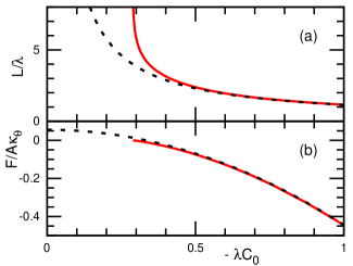
Figure 6: The cell length $L$ (a) and free energy $F$ (b) of inverted hexagonal $H_{II}$ phase with respect to the lamellar phase. The solid and dashed lines are obtained from the tilt model with variation calculus [Eqs. (21)] and the linear approximation [Eq. (19)], respectively.

First, we consider the free energy of a horizontal monolayer in Fig. 5. Here, we use the same coordinates as the simulations [${\bf n}=(0,0,1)$]. Since the molecules tilt only in the $x$ direction, i.e., $t_{y}=0$, the free energy of the monolayer is expressed as

$$F_{\rm{hex}}=2L_{y}\int_{0}^{L/2}\left[\frac{\kappa_{\rm{mo}}}{2}(t^{\prime}_{x}(x)-C_{0})^{2}+\frac{\kappa_{\rm\theta}}{2}t_{x}(x)^{2}\right]dx,$$ (18)

where $t^{\prime}_{x}=\partial t_{x}/\partial x$. The boundary conditions are $t_{x}(0)=0$ and $t_{x}(L/2)=-\tan(\pi/6)=-1/\sqrt{3}$, where $L$ is the side length of the hexagonal cell, $L=2L_{x}/3$. Hamm and Kozlov Hamm and Kozlov (1998) obtained

$$\frac{F_{\rm{hex}}}{A}=\frac{\kappa_{\rm{mo}}}{2}\Big{(}\frac{2}{\sqrt{3}L}+C_{0}\Big{)}^{2}+\frac{\kappa_{\rm\theta}}{18},$$ (19)

from the assumption that $t^{\prime}_{x}$ is constant. Here, we use $t_{x}(x)$ which minimizes $F_{\rm{hex}}$, instead of the constant $t^{\prime}_{x}$ assumption. The calculus of variation gives $t^{\prime\prime}_{x}(x)=(\kappa_{\rm\theta}/\kappa_{\rm{mo}})t_{x}(x)$. Hence, the molecules are tilted by

$$t_{x}(x)=-\frac{\sinh(x/\lambda)}{\sqrt{3}\sinh(L/2\lambda)},$$ (20)

where $\lambda=\sqrt{\kappa_{\rm{mo}}/\kappa_{\rm\theta}}$ is the characteristic length. Then the free energy is obtained as

$$\frac{F_{\rm{hex}}}{\kappa_{\rm{mo}}L_{y}}=\frac{\sinh(L/\lambda)}{3\lambda(\cosh(L/\lambda)-1)}+\frac{2C_{0}}{\sqrt{3}}+\frac{{C_{0}}^{2}L}{2}.$$ (21)

When the distance $L$ between the junctions is sufficiently large (i.e. $L\gg\lambda$), the first term on the R.H.S of Eq. (21) becomes $1/3\lambda$.

The free energy $F_{\rm{lam}}$ of the lamellar phase is given by $F_{\rm{lam}}/A=\kappa_{\rm{mo}}C_{0}^{2}/2$. The line tension of the branching junction is the energy required to form a junction per unit length, $\Gamma_{\rm{br}}L_{y}=3(F_{\rm{hex}}-F_{\rm{lam}})$, since one junction links six monolayers and one monolayer connects two junctions. Thus, $\Gamma_{\rm{br}}$ is given by

$$\Gamma_{\rm{br}}=\sqrt{\kappa_{\rm{mo}}\kappa_{\rm\theta}}(1+2\sqrt{3}\lambda C_{0}),$$ (22)

for $L\gg\lambda$.

Next, we compare the line tension of the tilt model with our simulation results. Molecular tilts are seen around the junctions in simulation snapshots [see Fig. 2(b)]. In our membrane model, the bending rigidity and spontaneous curvature of the monolayer are given by $\kappa_{\rm{mo}}/k_{\rm B}T\simeq 1.1(k_{\rm{bend}}+k_{\rm{tilt}})$ and $C_{0}\simeq\{\kappa_{\rm{bend}}/(\kappa_{\rm{bend}}+\kappa_{\rm{tilt}})\}C_{\rm{bd}}/\sigma$, respectively, as described in Sec. II.3. The tilt modulus $\kappa_{\rm\theta}$ is estimated as follows. When thermal fluctuations are neglected, the tilt energy $U_{\rm{tilt}}$ of a flat membrane with a constant tilt $t_{x}$ is given by

$$\frac{F_{\rm{tilt}}}{k_{\rm B}T}=\frac{k_{\rm{tilt}}}{4}{t_{x}}^{2}NN_{\rm{nb}}\langle w_{\rm{cv}}\rangle,$$ (23)

where $N_{\rm{nb}}$ is the mean number of neighboring molecules. Here the average $\langle({\bf t}\cdot\hat{\bf{r}})^{2}\rangle={\bf t}^{2}/d$ is used for isotropic unit vectors $\hat{\bf{r}}$ with a spatial dimension $d=2$. In the continuum limit, $F_{\rm{tilt}}$ should correspond to $F_{\rm{hex}}=\kappa_{\rm\theta}A{t_{x}}^{2}/2$ of the tilt model. Thus, $\kappa_{\rm\theta}$ is given by $\kappa_{\rm\theta}\simeq 2k_{\rm{tilt}}k_{\rm B}T/a_{xy}$ from $N_{\rm{nb}}=6$ and $\langle w_{\rm{cv}}\rangle=w_{\rm{cv}}(1.05\sigma)=0.61$. The line tension $\Gamma_{\rm{br}}$ calculated from Eq. (22) reproduces the simulation results very well for most of the parameter ranges in Fig. 4. The tilt model overestimates $\Gamma_{\rm{br}}$ for $k_{\rm{bend}}=0$ in Fig. 4(a). This deviation is likely caused by a too small characteristic length $\lambda$. It is less than the molecular diameter $\sigma$: $\lambda\simeq 0.8\sigma$ and $1.1\sigma$ at $k_{\rm{bend}}=0$ and $k_{\rm{bend}}=k_{\rm{tilt}}$, respectively, for the tensionless membranes with $a_{xy}\simeq 1.2\sigma^{2}$.

Finally, we discuss the stability of the inverted hexagonal $H_{II}$ phase using the tilt model. For $-\lambda C_{0}\leq 1/2\sqrt{3}$, the free energy per area $F_{\rm{hex}}/A$ monotonically decreases with increasing cell length $L$ [see Eq. (21)]. In this region, the lamellar phase ($L\to\infty$) is more stable than the $H_{II}$ phase. For $-\lambda C_{0}>1/2\sqrt{3}$, $F_{\rm{hex}}/A$ is minimum at finite $L$ and the $H_{II}$ phase is more stable than the lamellar phase. In this region, the line tension $\Gamma_{\rm{br}}$ is negative, and the $H_{II}$ hexagonal structure grows. Figure 6 shows $L$ and $(F_{\rm{hex}}-F_{\rm{lam}})/A$ obtained by the present method and the previous linear approximation Hamm and Kozlov (1998). Under the linear approximation, $(F_{\rm{hex}}-F_{\rm{lam}})/A=\kappa_{\rm\theta}/18-\kappa_{\rm{mo}}C_{0}^{2}/2$ with $L=-2/\sqrt{3}C_{0}$, so that the $H_{II}$ phase has a lower energy for $-\lambda C_{0}>1/3$. As $-\lambda C_{0}$ increases, the two lines in Fig. 6 approach each other. Thus, the linear approximation works well in the $H_{II}$ phase at $-\lambda C_{0}>0.5$, while not for $-\lambda C_{0}\lesssim 1/2\sqrt{3}$.

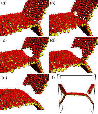
Figure 7: Sequential snapshots of the membrane rupture for $N=3072$, $\varepsilon=2$, $k_{\rm{bend}}=8$, $k_{\rm{tilt}}=8$, and $C_{\rm{bd}}=0$. (a) $t/\tau_{0}=2555$. (b) $t/\tau_{0}=2565$. (c) $t/\tau_{0}=2570$. (d) $t/\tau_{0}=2575$. (e), (f) $t/\tau_{0}=2580$.

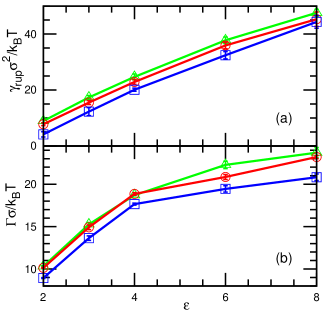
Figure 8: Parameter $\varepsilon$ dependence of (a) surface tension $\gamma_{\rm{cut}}$ of the membrane rupture and (b) the line tension of the membrane edge for $k_{\rm{bend}}=k_{\rm{tilt}}=8$. The triangles, circles, and squares represent data for $C_{\rm{bd}}=-0.2$, $0$, and $0.2$, respectively.

V Dynamics

V.1 Rupture

A membrane rupture occurs under sufficiently high surface tension $\gamma$. We investigated the rupture of branched membranes as $L_{y}$ is increased slowly at a rate $dL_{y}/dt=0.0002\sigma/\tau$. We checked that this rate is sufficiently small. No difference is detected when a rate twice as fast, i.e., $dL_{y}/dt=0.0004\sigma/\tau$, is used. Figure 7 shows the rupture of the branched membranes. A pore opens on the side of the branching junction and then expands along the junction. Since the junction is less stable than the middle of the bilayer membranes, the rupture always occurs on the side of the branching junction.

The surface tension $\gamma_{\rm{rup}}$ at the rupture is estimated from the extrapolation of the $L_{y}$-$\gamma$ line to the rupture point. As $\varepsilon$ increases, $\gamma_{\rm{rup}}$ increases linearly as shown in Fig. 8(a), although $\Gamma_{\rm{br}}$ is independent of $\varepsilon$. The line tension $\Gamma$ of the membrane edge also increases but it is not linear with respect to $\varepsilon$ [see Fig. 8(b)].

After the membrane rupture, a branched membrane becomes a line of a membrane edge and a bent membrane. The free energy of the former and latter states of the tensionless membranes are given by $F_{{\rm{br}}}/L_{y}=\Gamma_{\rm{br}}$ and $F_{{\rm{rup}}}/L_{y}=\Gamma+(\pi/6)\kappa/R$, respectively, where $R\sim 5\sigma$ is the curvature radius of the bent membrane. Thus, the branched membrane is kinetically stable for the rupture when $\Gamma_{\rm{br}}<\Gamma$ for $\gamma=0$. Furthermore, even when $F_{{\rm{br}}}>F_{{\rm{rup}}}$, the branched membrane can remain in a metastable state to overcome the free energy barrier to rupture. In the present spin molecular model, $\Gamma_{\rm{br}}$ and $\Gamma$ can be varied separately by $k_{\rm{tilt}}$ or $k_{\rm{bend}}$ and $\varepsilon$, respectively.

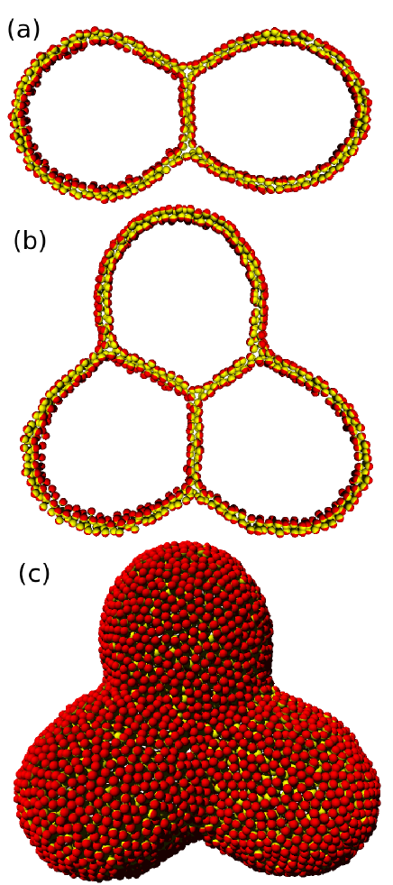
Figure 9: Branched structures in partially fused vesicles for $\varepsilon=8$, $k_{\rm{bend}}=8$, $k_{\rm{tilt}}=8$, and $C_{\rm{bd}}=0$. Sliced snapshots are shown in (a) two and (b) three hemifused vesicles for $N=4000$ and $N=6000$, respectively. (c) All molecules are shown for the snapshot in (b).

V.2 Fusion Intermediate

The branching junctions appear in the hemifusion diaphragm (HD) intermediate in membrane fusion [see Fig. 9(a)]. The HD intermediate was proposed in the original stalk model of membrane fusion Markin et al. (1984) and was observed in experiments Nikolaus et al. (2011) and in some of the molecular simulations Noguchi (2002); Marrink and Mark (2003); Smeijers et al. (2006); Gao et al. (2008). Here we focus on the structure of the HD intermediate and the detail of the fusion dynamics of the present model will be described somewhere else. Following the procedure in our previous fusion simulations Noguchi (2002), a spherical particle with a radius of $4\sigma$ is placed at the center of each vesicle and constant external forces are applied to the spherical particles. The membranes pinched by the particles are fused either directly or via the HD intermediate. The fusion dynamics are qualitatively similar to our previous simulations Noguchi (2002). When the HD is formed, we removed the spherical particles and then relaxed the vesicles to a stable structure. The resultant structures are shown in Fig. 9.

The HD of two vesicles has a circular branching junction. As the radius $R_{\rm{br}}$ of the branching junction increases, the bending energy is reduced because the flat membrane area also increases. However, the energy of the junction increases as $2\pi R_{\rm{br}}\Gamma_{\rm{br}}$. Thus, the radius is determined by the balance of these energies. Figures 9 (b) and (c) show the HD of three hemifused vesicles. Four lines of the branching junction meet at the centers of the front and back membranes. These vesicle shapes resemble the shape of soap bubbles. In the bubbles, competition between surface tension and pressure maintains their shapes, while in the vesicles, the bending energy and line tension play these roles.

VI Summary

We have studied the branching of bilayer membranes. The free energy of the branching junction can be treated as line tension when the distance between the junctions is sufficiently large. The line tension $\Gamma_{\rm{br}}$ of the junction is calculated from the pressure tensor in solvent-free molecular simulations. The simulation results agree well with the prediction of the tilt model.

The stability of the branching membranes depends on the boundary conditions. High surface tension induces membrane rupture on the side of the branching junction. In the hemifusion diaphragm intermediate, the branching junctions can be formed by the balance of the bending energy and line tension. Several kinds of proteins are known to modify membrane curvatures in living cells Baumgart et al. (2010); Phillips et al. (2009); Zimmerberg and Kozlov (2006). The branched structures induced by the absorption of a colloid Noguchi and Takasu (2002a), DNA Farago and Grønbech-Jensen (2009), and peptide Kawamoto and et al. (2011) have been reported in molecular simulations. The branching structures of the biomembranes may be stabilized or controlled by the absorption or insertion of proteins to the membranes in living cells.

The self-assembled structures of amphiphilic molecules can be clarified from the packing parameter Israelachvili (2011) of amphiphilic molecules or the spontaneous curvature of the monolayer. However, these quantities are not easy to measure. Alternatively, the line tension of the branching junction may be suitable to quantify the tendency of the amphiphilic molecules to form inverted structures.