Spinors: a Mathematica package for doing spinor calculus in General Relativity

Abstract

The Spinors software is a Mathematica package which implements 2-component spinor calculus as devised by Penrose for General Relativity in dimension 3+1. The Spinors software is part of the xAct system, which is a collection of Mathematica packages to do tensor analysis by computer. In this paper we give a thorough description of Spinors and present practical examples of use.

PROGRAM SUMMARY/NEW VERSION PROGRAM SUMMARY

Manuscript Title: Spinors: a Mathematica package for doing spinor calculus in General Relativity.
Authors: A. García-Parrado and J.M. Martín-García.
Program Title: Spinors.
Journal Reference:
Catalogue identifier:
Licensing provisions:
Programming language: Mathematica.
Computer: Any computer running Mathematica 7.0 or higher.
Operating system: Any operating system compatible with Mathematica 7.0 or higher.
RAM: 94Mb in Mathematica 8.0.
Number of processors used: 1.
Keywords: General Relativity, Spinor calculus.
Classification: Relativity and Gravitation.
External routines/libraries: Mathematica packages xCore, xPerm and xTensor which are part of the xAct system. These can be obtained at http://www.xact.es.
Nature of problem: Manipulation and simplification of spinor expressions in General Relativity.

Solution method: Adaptation of the tensor functionality of the xAct system for the specific situation of spinor calculus in four dimensional Lorentzian geometry.

Restrictions: The software only works on 4-dimensional Lorentzian space-times with metric of signature $(1,-1,-1,-1)$. There is no direct support for Dirac spinors.

Unusual features: Easy rules to transform tensor expressions into spinor ones and back. Seamless integration of abstract index manipulation of spinor expressions with component computations.

Running time: Under one second to handle and canonicalize standard spinorial expressions with a few dozen indices. (These expressions arise naturally in the transformation of a spinor expression into a tensor one or vice-versa).

* Items marked with an asterisk are only required for new versions of programs previously published in the CPC Program Library.

1 Introduction

The concept of spinor plays an important role in certain areas of mathematical and theoretical physics. Roughly speaking a spinor is a field which transforms under a spinor representation of a given symmetry group in our system. For example, if we are working in a pseudo-Riemannian manifold with a metric of signature $(p,q)$ ($p$ represents the number of $+1$ and $q$ the number of $-1$ entries in the canonical form of the metric), then a natural symmetry group is the group which transforms orthonormal frames into orthonormal frames. This group is $O(p,q)$ ($SO(p,q)$ if we restrict ourselves to transformations preserving the frame orientation). The spin group is then the universal covering of $SO(p,q)$ which, as is well-known, is $\mbox{\em Spin}(p,q)$ and hence spinors transform under irreducible representations of this group.

The above considerations are completely general and they enable us to introduce the notion of spinor field in any pseudo-Riemannian manifold admitting a spin structure. However, in the case of a 4-dimensional Lorentzian manifold (the space-time model in General Relativity) a more algebraic approach is desired. This approach was pioneered by Penrose [1] where he studied the main properties of the spinor algebra of those spinors arising from the spin group of $SO(1,3)$ and in addition he developed a calculus adapted to the particular spin vector bundle which one can define in a 4-dimensional Lorentzian manifold admitting a spin structure. Penrose’s spinor calculus revealed very useful in certain contexts of General Relativity (GR) where the use of tensor methods results in very cumbersome computations. Perhaps the best known example is the spinor formulation of the algebraic classification of the Weyl tensor (Petrov classification). The spinor form of the Weyl tensor is a totally symmetric 4-rank spinor and it is very easy to show that such a spinor can only admit four different algebraic types which are in correspondence with the four distinct Petrov types.

In this article we describe the Mathematica package Spinors which implements the spinor calculus in four dimensional Lorentzian geometry as conceived by Penrose. In this conception, spinors are tensor fields on a certain tensor bundle and therefore one can use the general ideas of tensor bundles to work with spinors. In particular the notion of spin covariant derivative, the curvature spinors or the relation between spinors and space-time tensors find here a natural formulation. An important part of this formulation is the notion of abstract index used to represent tensor fields on any tensor bundle. This representation of tensor fields has been adopted in the system xAct [2], which Spinors is part of. The system xAct is a system to do tensor analysis by computer in Mathematica, both by working with tensors as linear combination of basis tensors (component calculus) and by working with tensors as symbolic names with certain properties like rank or symmetry (abstract calculus). The system xAct consists of different modules tailored for different tasks and Spinors is one of these modules.

Other computer algebra systems support computations with spinors. For example in the context of Particle Physics we may quote the package Spinors@Mathematica [3] which can be used in the evaluation of scattering amplitudes at tree and loop level. The stand-alone package Cadabra [4] handles generic abstract spinor quantities in any dimension, with emphasis in Field Theory, but no special support for General Relativity or component computations. The Maple built-in package DifferentialGeometry has extensive support for component computations of multiple types, in particular the NP formalism, but no support for abstract tensor computations. Another Maple package handling the NP formalism is NPSpinor [5].

The paper is organised as follows: in section 2 we give a mathematical introduction to spinor calculus. The aim of this introduction is to set the notation and conventions which are followed by the Spinors implementation. Section 3 explains how the Spinors software fits into the xAct framework and section 4 presents a practical session with Spinors in which the main features of the program are shown by means of practical examples. The paper is finished in section 5 where a practical computation involving the Nester-Witten spinor and the Sparling identity is carried out with Spinors.

2 Mathematical preliminaries

In this section we give an overview of the spinor calculus in General Relativity, following a practical approach to introduce the subject and omitting most of the proofs (detailed studies can be found in e.g. [6, 7]). Let $\mathbf{L}$ be a 4-dimensional real vector space endowed with a real scalar product $g(\ ,\ )$ of Lorentzian signature and let $\mathbf{S}$ be a 2-dimensional complex vector space (complex conjugate of scalars will be denoted by an overbar). The vector space $\mathbf{S}$ is related to another complex vector space $\overline{\mathbf{S}}$ by an anti-linear, involutive transformation.

The vector space $\mathbf{L}$ and its dual ${\mathbf{L}}^{*}$ can be used as the starting point to build a tensor algebra in the standard fashion. Similarly a tensor algebra is built from $\mathbf{S}$, $\overline{\mathbf{S}}$ and their respective duals ${\mathbf{S}}^{*}$, $\overline{\mathbf{S}}^{*}$. We denote these algebras by $\mathfrak{T}(\mathbf{L})$, $\mathfrak{T}(\mathbf{S})$ and $\mathfrak{T}(\overline{\mathbf{S}})$ respectively . In this work abstract indices will be used throughout to denote tensorial quantities: in this way lowercase Latin indices $a,b,\dots$ will denote abstract indices on elements of $\mathfrak{T}(\mathbf{L})$ and capital Latin indices $A,B,\dots$ (resp. primed capital Latin indices $A^{\prime},B^{\prime},\dots$) will be used for abstract indices of elements in $\mathfrak{T}(\mathbf{S})$ (resp. $\mathfrak{T}(\overline{\mathbf{S}})$). The union of the tensor algebras $\mathfrak{T}(\mathbf{S})$, $\mathfrak{T}(\overline{\mathbf{S}})$ will be referred to as the spin algebra and its elements will be called spinors. One can also build tensor algebras by taking tensor products of elements in $\mathfrak{T}(\mathbf{L})$, $\mathfrak{T}(\mathbf{S})$ and $\mathfrak{T}(\overline{\mathbf{S}})$. Quantities in these tensor algebras will be referred to as mixed quantities and they will carry abstract indices of tensor and spinor type. All tensor algebras shall be regarded as complex vector spaces.

Since ${\mathbf{S}}$ is 2-dimensional, we deduce that the vector space of antisymmetric 2-spinors is 1-dimensional and therefore we can pick up a non-vanishing representative $\epsilon_{AB}$ which generates such a vector space. We define next a spinor $\widehat{\epsilon}^{AB}$ by the relation

$$\epsilon_{AB}\widehat{\epsilon}^{CB}=\delta^{\phantom{A}C}_{A}.$$ (1)

where $\delta_{A}^{\phantom{A}C}$ is the identity tensor (also known as the Kronecker delta) on the vector space $\mathbf{S}$. Indeed the spinors $\epsilon_{AB}$, $\widehat{\epsilon}^{AB}$ can be used to relate elements in $\mathbf{S}$ and elements in $\mathbf{S}^{*}$ in the following way

$$\xi^{A}\epsilon_{AB}=\xi_{B}\;,\quad\xi^{A}=\widehat{\epsilon}^{AB}\xi_{B}\;,$$ (2)

where $\xi^{A}$ is an arbitrary spinor in $\mathbf{S}$. Hence, the spinors $\epsilon_{AB}$ and $\widehat{\epsilon}^{AB}$ can be understood as a metric on ${\mathbf{S}}$ (symplectic metric) and its inverse and the operation shown in (2) is the standard “raising and lowering” of indices. These operations are extended to the full spinor algebra without difficulty. In particular we can raise the indices of $\epsilon_{AB}$ getting $\epsilon^{AB}=\widehat{\epsilon}^{AB}$ and from now on only the symbol $\epsilon$ will be used for the symplectic metric and its inverse. Note also the property

$$\delta^{A}_{\phantom{A}B}=-\delta_{B}^{\phantom{B}A}.$$ (3)

Here the quantity $\delta_{B}^{\phantom{B}A}$ is the Kronecker delta on $\mathbf{S}$ and $\delta^{A}_{\phantom{A}B}$ is a derived quantity obtained from it by the raising and lowering of indices. In particular this implies $\delta_{A}^{\phantom{A}A}=2$. The spinors $\epsilon_{AB}$, $\epsilon^{AB}$ and $\delta_{A}^{\phantom{A}B}$ all have counterparts (complex conjugates) defined in the algebra $\mathfrak{T}(\overline{\mathbf{S}})$.

It is possible to relate tensors and spinors by means of the soldering form. This is a mixed quantity $\sigma_{a}^{\phantom{a}AA^{\prime}}$ fulfilling the algebraic properties

$$\sigma^{a}_{\phantom{a}AA^{\prime}}\sigma_{aBB^{\prime}}=\epsilon_{BA}\bar{\epsilon}_{B^{\prime}A^{\prime}}\;,\quad\sigma^{a}_{\ AA^{\prime}}\sigma_{b}^{AA^{\prime}}=\delta^{a}_{\ b}\;,$$

$$\overline{\sigma_{a}^{\phantom{a}AA^{\prime}}}=\sigma_{a}^{\phantom{a}AA^{\prime}}.$$

The last of these properties implies that $\sigma^{a}_{\phantom{a}AA^{\prime}}$ is hermitian. This is only compatible with the metric signature $(1,-1,-1,-1)$. Choosing $\sigma^{a}_{\phantom{a}AA^{\prime}}$ anti-hermitian would be only compatible with the signature $(-1,1,1,1)$ [7]. These properties enable us to relate tensors and spinors in the following way

$$T^{A_{1}A_{1}^{\prime}\dots A_{p}A^{\prime}_{p}}_{\ B_{1}B^{\prime}_{1}\dots B_{q}B_{q}}=T^{a_{1}\dots a_{p}}_{\ b_{1}\dots b_{q}}\sigma^{b_{1}}_{\phantom{b_{1}}B_{1}B^{\prime}_{1}}\cdots\sigma^{b_{q}}_{\phantom{b_{q}}B_{q}B^{\prime}_{q}}\sigma_{a_{1}}^{\phantom{a_{1}}A_{1}A^{\prime}_{1}}\cdots\sigma_{a_{p}}^{\phantom{a_{p}}A_{p}A^{\prime}_{p}},$$

(4)

$$T^{a_{1}\dots a_{p}}_{\ b_{1}\dots b_{q}}=T^{A_{1}A_{1}^{\prime}\dots A_{p}A^{\prime}_{p}}_{\ B_{1}B^{\prime}_{1}\dots B_{q}B_{q}}\sigma_{b_{1}}^{\phantom{b_{1}}B_{1}B^{\prime}_{1}}\cdots\sigma_{b_{q}}^{\phantom{b_{q}}B_{q}B^{\prime}_{q}}\sigma^{a_{1}}_{\phantom{a_{1}}A_{1}A^{\prime}_{1}}\cdots\sigma^{a_{p}}_{\phantom{a_{p}}A_{p}A^{\prime}_{p}}.$$

(5)

where $T^{a_{1}\dots a_{p}}_{\ b_{1}\dots b_{q}}$ is an arbitrary tensor and $T^{A_{1}A_{1}^{\prime}\dots A_{p}A^{\prime}_{p}}_{\ B_{1}B^{\prime}_{1}\dots B_{q}B_{q}}$ its spinor counterpart

Another important algebraic property of the soldering form is

$$\sigma{}_{a}{}^{A}{}_{A^{\prime}}\sigma{}_{b}{}_{A}{}_{C^{\prime}}+\sigma\ {}_{a}{}_{A}{}_{C^{\prime}}\sigma{}_{b}{}^{A}{}_{A^{\prime}}=g{}_{a}{}_{b}\ \overline{\epsilon}{}_{A^{\prime}}{}_{C^{\prime}}.$$ (6)

This equation is a direct consequence of the irreducible decomposition of the product $\sigma{}_{a}{}^{A}{}_{A^{\prime}}\sigma{}_{b}{}_{A}{}_{C^{\prime}}$ according to theorem 1 below and the algebraic properties of the soldering form. Starting from (6) we can derive formulas for the products of soldering forms with all their spinor indices contracted (these are useful to translate spinor expressions into tensor ones). For example

$$\sigma{}_{a}{}_{A}{}_{A^{\prime}}\sigma{}_{b}{}^{A}{}_{C^{\prime}}\sigma{}_{c}{}^{D}{}^{C^{\prime}}\sigma{}_{d}{}_{D}{}^{A^{\prime}}=$$

$$\frac{1}{2}(\mbox{i}\eta{}_{c}{}_{d}{}_{a}{}_{b}+g{}_{a}{}_{b}g{}_{c}{}_{d}+g{}_{c}{}_{b}g{}_{d}{}_{a}-g{}_{c}{}_{a}g{}_{d}{}_{b})\;,$$ (7)

where $\eta_{abcd}$ is the volume form of the metric $g_{ab}$. It is possible to generalise this formula for the case of a product of more soldering forms. These can be written as contracted products of the quantity

$$G_{abcd}\equiv\frac{1}{2}(\mbox{i}\eta{}_{a}{}_{b}{}_{c}{}_{d}+g{}_{a}{}_{d}g{}_{b}{}_{c}-g{}_{a}{}_{c}g{}_{b}{}_{d}+g{}_{a}{}_{b}g{}_{c}{}_{d}).$$ (8)

Combining eq. (7) and its complex conjugate we obtain the spinor counterpart of $\eta_{abcd}$, written as follows

$$\eta{}_{a}{}_{b}{}_{c}{}_{d}\sigma{}^{a}{}_{A}{}_{A^{\prime}}\sigma{}^{b}{}_{B}{}_{B^{\prime}}\sigma{}^{c}{}_{C}{}_{C^{\prime}}\sigma{}^{d}{}_{D}{}_{D^{\prime}}=$$

$$i(\epsilon{}_{A}{}_{C}\epsilon{}_{B}{}_{D}\overline{\epsilon}{}_{A^{\prime}}{}_{D^{\prime}}\ \overline{\epsilon}{}_{B^{\prime}}{}_{C^{\prime}}-\epsilon{}_{A}{}_{D}\epsilon{}_{B}{}_{C}\overline{\epsilon}{}_{A^{\prime}}{}_{C^{\prime}}\overline{\epsilon}{}_{B^{\prime}}{}_{D^{\prime}}).$$ (9)

We finish this review about spinor algebra by recalling an important result dealing with the decomposition of an arbitrary spinor into irreducible parts under the Lorentz group [6].

Theorem 1.

Any spinor $\xi_{A_{1}\cdots A_{p}B^{\prime}_{1}\cdots B^{\prime}_{q}}$, $p,q\in\mathbb{N}$ can be written as the sum of a totally symmetric spinor $\xi_{(A_{1}\cdots A_{p})(B^{\prime}_{1}\cdots B^{\prime}_{q})}$ plus terms which are products of the spin metric $\epsilon_{AB}$ (or its complex conjugate $\bar{\epsilon}_{A^{\prime}B^{\prime}}$) times totally symmetric spinors of lower rank.

2.1 Spinor calculus

So far all our considerations were algebraic in nature, but we can also perform our construction for the case of a Lorentzian manifold $(\mathcal{M},g)$ as follows: the construction performed in previous paragraphs is carried out taking as vector space ${\mathbf{L}}$ the tangent space $T_{p}(\mathcal{M})$ of an arbitrary point $p\in\mathcal{M}$ which is endowed with the Lorentzian scalar product $g|_{p}$. In this way it is possible to introduce a complex vector space $\mathbf{S}_{p}$ and a quantity $\sigma_{a}^{\phantom{a}AA^{\prime}}|_{p}$. Now the set $S(\mathcal{M})\equiv\bigcup_{p\in{\mathcal{M}}}{\mathbf{S}}_{p}$ is a vector bundle with the manifold $\mathcal{M}$ as the base space and the group of linear transformations on $\mathbb{C}^{2}$ as the structure group. We will call this vector bundle the spin bundle and the sections of $S(\mathcal{M})$ are the contravariant rank-1 spinor fields on ${\mathcal{M}}$. We can now define the tensor algebras $\mathfrak{T}^{r}_{s}(T_{p}({\mathcal{M}}))$, $\mathfrak{T}^{R}_{S}(\mathbf{S}_{p})$ and, use them to construct vector bundles with $\mathcal{M}$ as the base manifold. These bundles are tensor bundles and we denote each of these tensor bundles by $\mathfrak{S}^{r,R}_{s,S}(\mathcal{M})$, where the meaning of the labels $r$, $R$, $s$, $S$ is the obvious one. In general we will suppress these labels and use just the notation $\mathfrak{S}(\mathcal{M})$ as a generic symbol for these tensor bundles. Sections on $\mathfrak{S}(\mathcal{M})$ are written using abstract indices and we follow the same conventions as in the case of the vector spaces ${\mathbf{L}}$ and ${\mathbf{S}}$. Sections of any of the bundles $\mathfrak{S}^{0,R}_{0,S}(\mathcal{M})$ are called spinor fields or simply spinors. As usual there is a complex conjugate counterpart of this bundle, denoted by $\overline{\mathfrak{S}(\mathcal{M})}$.

Definition 1 (Spin structure).

If the quantity $\sigma_{a}^{\phantom{a}AA^{\prime}}|_{p}$ varies smoothly on the manifold $\mathcal{M}$, then one can define a smooth section, denoted by $\sigma_{a}^{\phantom{a}AA^{\prime}}$. When this is the case we call the smooth section $\sigma_{a}^{\phantom{a}AA^{\prime}}$ a smooth spin structure on the Lorentzian manifold $({\mathcal{M}},g)$.

Clearly a spin structure can be always defined in a neighbourhood of any point $p\in\mathcal{M}$ but further topological restrictions are required if the spin structure is to be defined globally (see e.g. [8]).

We turn now to the study of covariant derivatives defined on the bundles $\mathfrak{S}(\mathcal{M})$, $\overline{\mathfrak{S}(\mathcal{M})}$. Let $D_{a}$ denote such a covariant derivative. Then the operator $D_{a}$ can act on any quantity with tensor indices and/or spinor indices. As a result, when $D_{a}$ is restricted to quantities having only tensor indices we recover the standard notion of covariant derivative acting on tensor fields of $\mathcal{M}$. If $D_{a}$ is restricted to quantities having only spinor indices then $D_{a}$ is the covariant derivative acting on spinor fields. The consequence of this is that the connection coefficients and the curvature of $D_{a}$ will be divided in two groups: quantities arising from the tensorial part and quantities arising from the spinorial part. The group arising from the tensorial part consists of the Christoffel symbols/Ricci rotation coefficients and the Riemann tensor of the covariant derivative restricted to the tangent bundle $T(\mathcal{M})$. The group coming from the spinorial part contains the connection components and the curvature tensor of the covariant derivative restricted to the spin bundle $S(\mathcal{M})$ (or $\overline{S(\mathcal{M})}$). We will refer to these as the inner connection and the inner curvature respectively. See [7, 9] for an in-depth discussion of these concepts.

Definition 2 (Spin covariant derivative).

Suppose that $\mathfrak{S}(\mathcal{M})$ admits a spin structure $\sigma_{b}^{\phantom{b}AA^{\prime}}$. We say that a covariant derivative $D_{a}$ defined on $\mathfrak{S}(\mathcal{M})$ is compatible with the spin structure $\sigma_{b}^{\phantom{b}AA^{\prime}}$ if it fulfils the property

$$D_{a}\sigma_{b}^{\phantom{a}AA^{\prime}}=0.$$ (10)

The covariant derivative $D_{a}$ is then called a spin covariant derivative with respect to the spin structure $\sigma_{b}^{\phantom{a}AA^{\prime}}$.

Given that any quantity antisymmetric in two spinor indices must contain the spin metric as a factor we have

$$D_{a}\epsilon_{AB}=\lambda_{a}\epsilon_{AB}\;,\quad\lambda_{a}\equiv\epsilon^{AB}D_{a}\epsilon_{AB}\;,$$ (11)

where $D_{a}$ is any covariant derivative defined on the bundle $\mathfrak{S}(\mathcal{M})$. When $D_{a}$ is in addition a spin covariant derivative then, combining (10) and (11) we easily deduce the additional properties

$$D_{a}\sigma^{b}_{\phantom{b}AA^{\prime}}=0\;,\quad D_{c}g_{ab}=(\lambda_{c}+\bar{\lambda}_{c})g_{ab}.$$ (12)

The last equation implies that any spin convariant derivative gives rise to a semi-metric connection [10] when restricted to the space-time tensor bundle. If furthermore $D_{a}$ has no torsion, then it is known as a Weyl connection. The spin covariant derivative gets fixed if we demand additional properties on it (see e. g. [6])

Theorem 2.

There is one and only one torsion-free spin covariant derivative $\nabla_{a}$ with respect to the spin structure $\sigma_{a}^{\phantom{a}AA^{\prime}}$ which fulfills the property

$$\nabla_{a}\epsilon_{AB}=0.$$ (13)

Acting with such $\nabla_{a}$ on (6) gives

$$\nabla_{a}g_{bc}=0,$$ (14)

which shows that the restriction of $\nabla_{a}$ to quantities with tensorial indices is just the Levi-Civita covariant derivative of $g_{ab}$.

Consider now any spinor field $\xi^{A}$ and any spin covariant derivative $D_{a}$. Then the commutation of $D_{a}$, $D_{b}$ acting on $\xi^{A}$ is given by [7]

$$D_{a}D_{b}\xi^{B}-D_{b}D_{a}\xi^{B}-T^{r}_{\phantom{r}ab}D_{r}\xi^{B}=F_{abR}^{\phantom{abC}B}\xi^{C}$$ (15)

where $T^{r}_{\phantom{r}ab}$ is the torsion of $D_{a}$. The mixed quantity $F_{abA}^{\phantom{abA}B}$ is the inner curvature mentioned above. It is antisymmetric in the tensorial indices and it fulfils the Bianchi identity [7]

$$D_{[a}F_{bc]\phantom{B}A}^{\phantom{bc]}B}+T_{\phantom{r}[ab}^{r}F_{c]r\phantom{B}A}^{\phantom{c]r}B}=0.$$ (16)

The spinor counterpart of the inner curvature is represented by $F_{CC^{\prime}DD^{\prime}A}^{\phantom{CC^{\prime}DD^{\prime}A}B}$ and it can be decomposed as follows

$$F_{CC^{\prime}DD^{\prime}AB}=X_{ABCD}\bar{\epsilon}_{C^{\prime}D^{\prime}}+\Phi_{ABC^{\prime}D^{\prime}}\epsilon_{CD}.$$ (17)

The spinors $X_{ABCD}$ and $\Phi_{ABC^{\prime}D^{\prime}}$ are called curvature spinors and they enjoy the symmetries

$$X_{AB(CD)}=X_{ABCD}\;,\quad\Phi_{AB(C^{\prime}D^{\prime})}=\Phi_{ABC^{\prime}D^{\prime}}.$$ (18)

We can also introduce a spinor $T^{AA^{\prime}}_{\phantom{AA^{\prime}}BB^{\prime}CC^{\prime}}$ representing the torsion. Its irreducible decomposition reads

$$T^{AA^{\prime}}_{\phantom{AA^{\prime}}BB^{\prime}CC^{\prime}}=\Omega^{AA^{\prime}}_{\phantom{AA^{\prime}}BC}\bar{\epsilon}_{B^{\prime}C^{\prime}}+\bar{\Omega}^{AA^{\prime}}_{\phantom{AA^{\prime}}B^{\prime}C^{\prime}}\epsilon_{BC},$$ (19)

where $\Omega_{AA^{\prime}BC}$ is the torsion spinor and it fulfills the symmetries

$$\Omega_{AA^{\prime}(BC)}=\Omega_{AA^{\prime}BC}.$$ (20)

The inner curvature and the Riemann tensor of $D_{a}$ are indeed related. To find the relation between them one computes the Ricci identity for an arbitrary vector $V^{a}$ and then particularises it for the special case in which $V^{a}=\sigma^{a}_{\phantom{a}AA^{\prime}}\xi^{A}\xi^{A^{\prime}}$. The result is

$$R_{abc}^{\phantom{abc}d}=(F_{abC}^{\phantom{abC}D}\bar{\epsilon}_{C^{\prime}}^{\phantom{C^{\prime}}D^{\prime}}+\bar{F}_{abC^{\prime}}^{\phantom{abC^{\prime}}D^{\prime}}\epsilon_{C}^{\phantom{C}D})\sigma_{c}^{\phantom{c}CC^{\prime}}\sigma^{d}_{\phantom{d}DD^{\prime}}.$$ (21)

In the important particular case of a torsion-free connection which is compatible with the metric (Levi-Civita connection) the curvature spinors gain further symmetries. These are

$$X_{(AB)CD}=X_{ABCD}\;,\quad X_{ABCD}=X_{CDAB}\;,$$

$$\Phi_{(AB)C^{\prime}D^{\prime}}=\Phi_{ABC^{\prime}D^{\prime}}.$$

Given these additional symmetries we find that the spinor $\Phi_{ABC^{\prime}D^{\prime}}$ is already in its irreducible form and it is called the Ricci spinor. The irreducible decomposition of the spinor $X_{ABCD}$ yields

$$X_{ABCD}=\Psi_{ABCD}+\Lambda(\epsilon_{AD}\epsilon_{BC}+\epsilon_{AC}\epsilon_{BD}),$$ (22)

where $\Psi_{ABCD}$ is a totally symmetric spinor called the Weyl spinor and $\Lambda$ is related to the scalar curvature by the formula $\Lambda=R/24$. The curvature spinors and the torsion spinor are defined up to a constant scalar factor.

When working with a spin covariant derivative $D_{a}$ it is convenient to introduce the differential operator

$$D_{AA^{\prime}}\equiv\sigma^{a}_{\phantom{a}AA^{\prime}}D_{a}\;,$$ (23)

which enables us to render any expression containing spin covariant derivatives as an expression containing only spinor indices. Also the commutation $D_{AA^{\prime}}D_{BB^{\prime}}-D_{BB^{\prime}}D_{AA^{\prime}}$ can be formally decomposed into irreducible parts as follows

$$D_{AA^{\prime}}D_{BB^{\prime}}-D_{BB^{\prime}}D_{AA^{\prime}}=\overline{\epsilon}_{A^{\prime}B^{\prime}}\raise-1.13809pt\hbox{\large$\Box$}_{AB}+\epsilon_{AB}\raise-1.13809pt\hbox{\large$\Box$}_{A^{\prime}B^{\prime}},$$ (24)

where

$$\raise-1.13809pt\hbox{\large$\Box$}_{AB}\equiv D_{(A|A^{\prime}}D^{A^{\prime}}_{\phantom{A^{\prime}}|B)}\;,\quad\raise-1.13809pt\hbox{\large$\Box$}_{A^{\prime}B^{\prime}}\equiv D_{A(A^{\prime}}D^{A}_{\phantom{A}B^{\prime})}\;,$$ (25)

are linear differential operators. The action of these operators on a spinor of any rank is obtained from the spinor expression of the Ricci identity of $D_{a}$ and the expression of the Riemann tensor in terms of the curvature spinors. The results for the case of a rank-1 spinor are

$$\raise-1.13809pt\hbox{\large$\Box$}_{BC}\xi^{D}=X_{D\phantom{A}BC}^{\phantom{D}A}\xi^{D}-\Omega^{A^{\prime}D}_{\phantom{A^{\prime}D}BC}D_{DA^{\prime}}\xi^{A}$$ (26)

3 The package Spinors and its relation to xAct

The package Spinors is a Mathematica package which implements the spinor calculus as described in the previous section. Spinors is part of xAct [2], which is a system to do tensor analysis by computer written mostly in the Mathematica programming language with a smaller part in C. The composition is roughly 16000 lines of Mathematica code and 2700 lines of C code. As of October 2011 the version of xAct is 1.0.3. and the complete system is free software available under the terms of the GPL license.

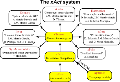
Figure 1: Graphical depiction of the xAct packages and their dependencies. The packages coloured in yellow can be regarded as the system Kernel and have been developed by J.M. Martín-García.

The system xAct is organised as a suite of inter-dependent Mathematica packages which can be regarded as different-purpose modules loadable on-demand. The packages and the relations among them are depicted in figure 1. The arrows indicate which packages of the suite a given package relies upon and we can see that there are three packages (xCore, xPerm and xTensor) which act as kernel for the whole implementation. This means that these packages yield the basic framework to set up any computation requiring tensor analysis. In addition the module xperm.c is a piece of code in C language devised to speed-up the group theoretical computations needed to canonicalize tensor expressions [11]. When loading any other package of xAct, all the necessary packages are loaded sequentially, following the order shown in figure 1.

The xAct system can be enlarged by adding new packages for specific purposes, as long as the dependencies just described are kept. Some of the packages shown in figure 1 have been already described in the literature. This is the case of xPerm [11], Invar [12, 13] and xPert [14]. In addition to these references, each package included in xAct has a documentation file, which explains its main features and contains a tutorial.

The xAct system provides support to define and work with general vector bundles on any manifold and dimension. This means that the main features of spinor algebra and spinor calculus are generically built into xAct for any dimension. However, in the particular case of Lorentzian geometry in dimension four, extra features arise as described in section 2 and hence it was necessary to develop a new package to take care of these features. For example the presence of the antisymmetric metric $\epsilon_{AB}$ forces us to be careful with the conventions to raise and lower indices. Also we need to decide which index configuration represents the basic Kronecker delta and which index configuration represents a derived quantity. In our case all these conventions were laid in eqs. (2)-(3) and one needs to take these particular conventions to the software implementation. Another delicate task is the 2-index representation of the spin covariant derivatives and their properties (eqs. (23)- (24)). This representation only occurs in the spinor calculus and hence we had to code the corresponding properties explicitly for the Spinors package. Finally the formulae relating spinors and tensors had to be studied and coded from scratch (this was perhaps one of the most time-consuming tasks in the development of Spinors). The conclusion of all of this is that spinor theory is complex enough to develop a new package for the xAct suite.

The package spinors has already been used by a number of authors in their research. An example of this is the invariant construction of Kerr initial data in [15, 16] (see also [17] for a generalisation of these results). The present authors have also used Spinors in the investigation of the invariant properties of type D vacuum solutions of the Einstein’s field equations [18].

4 Working with Spinors

Assuming xAct has been installed one loads Spinors in a Mathematica session by typing

In[1]:=   << xAct`Spinors`
------------------------------------------------------------

Package xAct‘Spinors‘ version 1.0.2, {2011,10,25}

CopyRight (C) 2006-2011, Alfonso Garcia-Parrado Gomez-Lobo and Jose M. Martin-Garcia, under the General Public License. ------------------------------------------------------------

This will load the package Spinors together with the other packages of the xAct suite which Spinors relies on. These are xCore, xPerm and xTensor (see section 3 and figure 1). In this work we will only explain the features of these packages which are required for our implementation and we refer the reader to their documentation for further details.

Next we need to declare a 4-dimensional Lorentzian manifold by means of the standard xAct machinery:

In[2]:=   DefManifold[M4, 4, {a, b, c, d, f, h, p}]
In[3]:=   DefMetric[{1,3,0}, g[-a,-b], CD]

The list {a, b, c, d, f, h, p} corresponds to the space-time abstract indices which will be used in tensor expressions and the list {1,3,0} in DefMetric serves to indicate the canonical form of the metric tensor g (its canonical form contains once +1, three times -1 and zero times 0, thus it corresponds to a Lorentzian metric). The symbol CD represents the Levi-Civita connection compatible with the metric g and in addition a number of quantities (the Riemann tensor, the Ricci tensor, the Weyl tensor, etc) are also created automatically after issuing the command DefMetric.

So far we have used commands belonging to xTensor and we have now the set-up necessary to start working with Spinors. The first step is the introduction of a spin structure. This is achieved as follows

In[4]:=   DefSpinStructure[g, Spin, {A, B, C, D, F, P}, $\epsilon$, $\sigma$, CDe]

Several new objects are defined alongside this command. These are the spin bundle Spin, its abstract indices {A, B, C, D, F, P}, the spin metric $\epsilon$, the soldering form $\sigma$ and the spin covariant derivative CDe compatible with both the space-time metric g and the spin metric $\epsilon$. The spin bundle Spin  ​  together with its structures and the curvature spinors are automatically defined with this command. For example the Weyl and Ricci spinors are

In[5]:=   {PsiCDe[-A, -B, -C, -D], PhiCDe[-A, -B, -C  ​ , -D  ​  ]}
Out[5]=   $\{\Psi[\nabla]_{\rm ABCD},\;\Phi[\nabla]_{\rm ABC\;\rule{0.5123pt}{4.26773pt}\!\raisebox{2.84526pt}{\rule{2.27626pt}{0.56917pt}}D\;\rule{0.5123pt}{4.26773pt}\!\raisebox{2.84526pt}{\rule{2.27626pt}{0.56917pt}}}\}$

Additional options controlling the displayed form of the different quantitites automatically defined can be supplied to DefSpinStructure. For example we may add the options

SpinorPrefix-> SP,   SpinorMark-> "S".

The symbol SP will be prepended to the tensor (spinor) counterpart of any spinor (tensor) and the string "S" will be used in the displayed representation (see below for explicit examples). From now on it will be understood that these options were used in the command DefSpinStructure above.

Primed indices are entered with the “dagger” symbol   ​  (entered via the keyboard shortcut

In[6]:=   SP​$\underbracket{\ \ }_{\ }$RicciCD[-A, -A  ​ , -B, -B  ​ ]
Out[6]=   $S{\rm R}[\nabla]_{\rm AA\;\rule{0.5123pt}{4.26773pt}\!\raisebox{2.84526pt}{\rule{2.27626pt}{0.56917pt}}BB\;\rule{0.5123pt}{4.26773pt}\!\raisebox{2.84526pt}{\rule{2.27626pt}{0.56917pt}}}$

The linking symbol “$\underbracket{\ \ }_{\ }$” (entered through the key combinations

In[7]:=   PrintAs[A  ​ ] ^∧="A^′"; PrintAs[B  ​ ] ^∧="B^′";
PrintAs[C  ​ ] ^∧="C^′"; PrintAs[D  ​ ] ^∧="D^′"; PrintAs[F  ​ ] ^∧="F^′";

Also we can modify the printing output of any tensor or spinor

In[8]:=   PrintAs[$\epsilon\;\rule{0.5123pt}{4.26773pt}\!\raisebox{2.84526pt}{\rule{2.27626pt}{0.56917pt}}$] ^∧= "$\bar{\epsilon}$";

The command Decomposition can be used to find the decomposition into irreducible parts of any other curvature spinor (it is possible to indicate the curvature spinor being decomposed as an additional argument). For example

In[9]:=   SP​$\underbracket{\ \ }_{\ }$RiemannCD[-A, -A  ​ , -B, -B  ​ ,-C, -C  ​ , -D, -D  ​ ]
// Decomposition
Out[9]=   $\Psi[\triangledown]\;\rule{0.5123pt}{4.26773pt}\!\raisebox{2.84526pt}{\rule{2.27626pt}{0.56917pt}}_{\rm A^{\prime}B^{\prime}D^{\prime}C^{\prime}}\epsilon_{\rm AB}\epsilon_{\rm CD}-\Phi[\triangledown]_{\rm ABD^{\prime}C^{\prime}}\epsilon_{\rm DC}\bar{\epsilon}_{\rm A^{\prime}B^{\prime}}-2\Lambda[\triangledown](\epsilon_{\rm AD}\epsilon_{\rm BC}\bar{\epsilon}_{\rm A^{\prime}D^{\prime}}\bar{\epsilon}_{\rm B^{\prime}C^{\prime}}-\epsilon_{\rm AC}\epsilon_{\rm BD}\ \bar{\epsilon}_{\rm A^{\prime}C^{\prime}}\bar{\epsilon}_{\rm B^{\prime}D^{\prime}})-\ \Phi[\triangledown]_{\rm DCA^{\prime}B^{\prime}}\epsilon_{\rm AB}\ \bar{\epsilon}_{\rm D^{\prime}C^{\prime}}+\Psi[\triangledown]_{\rm ABDC}\bar{\epsilon}_{\rm A^{\prime}B^{\prime}}\bar{\epsilon}_{\rm C^{\prime}D^{\prime}}$

The spin covariant derivative CDe can be handled as a 2-index covariant derivative …

In[10]:=   CDe[-F,-F  ​ ]@PsiCDe[-A,-B,-C,-D]
Out[10]=   $\nabla_{\rm FF^{\prime}}\Psi[\nabla]_{\rm ABCD}$

.. or as a covariant derivative in a vector bundle

In[11]:=   SeparateSolderingForm[][%]
Out[11]=   $\sigma^{\rm a}{}_{\rm FF^{\prime}}\triangledown_{\rm a}\Psi[\triangledown]_{\rm ABCD}$.

The command SeparateSolderingForm enables us to transform spinor indices into tensor ones (cf. §4.1 for more details about this).

Spinors are defined by means of DefSpinor, which is just a special call to the xAct command DefTensor (by default the option Dagger->Complex is assumed).

In[12]:=   DefSpinor[$\kappa$[-A, -A  ​ ], M4]
** DefTensor: Defining tensor $\kappa$[-A, -A  ​ ].
** DefTensor: Defining tensor $\kappa$  ​ [-A  ​ , -A].

If one wishes to work with Hermitian spinors then this is done by using the option Dagger -> Hermitian on the command DefSpinor. Under this assumption one has that $\kappa$[-A,-A  ​ ] is invariant under complex conjugation

In[13]:=   $\kappa$[-A,-A  ​ ] // Dagger // InputForm
Out[13]=   $\kappa$[-A,-A  ​ ]

The canonicalizer of xAct is ToCanonical and it can deal with the canonicalization of spinor expressions without any additional user input. It is beyond the present article to explain the workings of the canonicalization procedure and the reader is referred to [11] and the xTensor documentation for additional details. Similarly, the xAct command ContractMetric takes care automatically of the conventions for raising and lowering indices in spinor expressions. We present next some explicit examples about these issues

In[14]:=   DefSpinor[$\mu$[A], M4]
** DefTensor: Defining tensor $\mu$[A].
** DefTensor: Defining tensor $\mu$  ​ [A  ​ ].

In[15]:=   {$\mu$[-B]$\epsilon$[A,B],$\mu$[B]$\epsilon$[-B,-A],$\epsilon$  ​ [C  ​ ,A  ​ ] CDe[-A,-A  ​ ]@$\mu$[-B]}
Out[15]=   $\{\epsilon^{\rm AB}\mu_{\rm B},\ \epsilon_{\rm BA}\mu^{\rm B},\ \bar{\epsilon}^{\rm C^{\prime}A^{\prime}}\triangledown_{\rm AA^{\prime}}\mu_{\rm B}\}$

In[16]:=   ContractMetric[%]
Out[16]=   $\{\mu^{\rm A},\ \mu_{\rm A},\ \triangledown_{\rm A}{}^{\rm C^{\prime}}\mu_{\rm B}\}$

In[17]:=   { $\mu$[A]$\mu$[-A], $\kappa$[-A, -B  ​ ]$\mu$[B  ​ ], CDe[-F, -F  ​ ]@CDe[-A, F  ​ ]@PsiCDe[-B, -C, -D, -P]+ CDe[-F, F  ​ ]@CDe[-A, -F  ​ ]@PsiCDe[-B, -C, -D,-P] }
Out[17]=   $\{\mu_{\rm A}\mu^{\rm A},\ \kappa_{\rm AB^{\prime}}\bar{\mu}^{\rm B^{\prime}},\ \triangledown_{\rm FF^{\prime}}\triangledown_{\rm A}{}^{\rm F^{\prime}}\Psi[\triangledown]_{\rm BCDP}+\triangledown_{\rm F}{}^{\rm F^{\prime}}\triangledown_{\rm AF^{\prime}}\Psi[\triangledown]_{\rm BCDP}\}$

In[18]:=   ToCanonical[%]
Out[18]=   $\{0,\ -\kappa_{\rm A}{}^{\rm B^{\prime}}\bar{\mu}_{\rm B^{\prime}},\ 0\}$

Also the commutation of the spin covariant derivatives shown in (24) is implemented

In[19]:=   CDe[-C,-C  ​ ]@CDe[-B,-B  ​ ]@$\kappa$[-A,-A  ​ ]-
CDe[-B,-B  ​ ]@CDe[-C,-C  ​ ]@$\kappa$[-A,-A  ​ ]
Out[19]=   - $\triangledown_{\rm BB^{\prime}}\triangledown_{\rm CC^{\prime}}\kappa_{\rm AA^{\prime}}+\triangledown_{\rm CC^{\prime}}\triangledown_{\rm BB^{\prime}}\kappa_{\rm AA^{\prime}}$

In[20]:=   SortSpinCovDs[%,CDe]
Out[20]=   $\bar{\epsilon}_{\rm C^{\prime}B^{\prime}}(\square[\triangledown]_{\rm CB}\kappa_{\rm AA^{\prime}})+\epsilon_{\rm CB}(\square[\triangledown]_{\rm C^{\prime}B^{\prime}}\kappa_{\rm AA^{\prime}})$

The differential operator $\raise-1.13809pt\hbox{\large$\Box$}_{AB}$ can be written in terms of the spin 2-index covariant derivatives as illustrated in the following example

In[21]:=   BoxCDe[-A,-B]@$\kappa$[-C,-C  ​ ]
Out[21]=   $\square[\nabla]_{\rm AB}\kappa_{\rm CC^{\prime}}$

In[22]:=   BoxToCovD[%,BoxCDe]
Out[22]=   $\frac{1}{2}(\nabla_{\rm AA^{\prime}}\nabla_{\rm B}{}^{\rm A^{\prime}}\kappa_{\rm CC^{\prime}}+\nabla_{\rm BA^{\prime}}\nabla_{\rm A}{}^{\rm A^{\prime}}\kappa_{\rm CC^{\prime}})$

In[23]:=   BoxToCurvature[%%,BoxCDe]
Out[23]=   - $\Phi[\nabla]_{\rm ABA^{\prime}C^{\prime}}\kappa_{\rm C}{}^{\rm A^{\prime}}-X[\nabla]_{\rm DCAB}\kappa^{\rm D}{}_{\rm C^{\prime}}$

In our previous examples we worked with the spin covariant derivative arising from the Levi-Civita connection but we can introduce other arbitrary spin covariant derivatives. For example

In[24]:=   DefSpinCovD[nb[-a], $\sigma$, SymbolOfCovD-> {"|","D"}, Torsion->True]

As we see in the example the command DefSpinCovD shares some similarities with the xTensor command DefCovD. In addition to the spin covariant derivative output symbols, we also need to specify the spin structure which the spin covariant derivative is compatible with (this is $\sigma$ in our example). Hence

In[25]:=   {nb[-a]@$\sigma$[b, -A, -A  ​ ], nb[-a]@$\sigma$[-b, A, A  ​ ] }
Out[25]=   {0, 0}

Also, a number of quantities are automatically defined in addition to the spin covariant derivative nb. Since we used the option Torsion->True the torsion is among those and one can work with both its tensor and spinor forms.

In[26]:=   SeparateSolderingForm[]@Torsionnb[a,-b,-c]
Out[26]=   ${\rm ST}[{\rm D}]^{\rm AA^{\prime}}{}_{\rm BB^{\prime}CC^{\prime}}\sigma^{\rm a}{}_{\rm AA^{\prime}}\sigma_{\rm b}{}^{\rm BB^{\prime}}\sigma_{\rm c}{}^{\rm CC^{\prime}}$

In[27]:=   PutSolderingForm@Decomposition@%
Out[27]=   $\epsilon^{\rm AD}\bar{\epsilon}^{\rm A^{\prime}D^{\prime}}(\Omega[{\rm D}]\;\rule{0.5123pt}{4.26773pt}\!\raisebox{2.84526pt}{\rule{2.27626pt}{0.56917pt}}_{\rm DD^{\prime}B^{\prime}C^{\prime}}\epsilon_{\rm BC}+\Omega[{\rm D}]_{\rm D^{\prime}DBC}\bar{\epsilon}_{\rm B^{\prime}C^{\prime}})$

In[28]:=   ContractMetric@%
Out[28]=   $\Omega[{\rm D}]\;\rule{0.5123pt}{4.26773pt}\!\raisebox{2.84526pt}{\rule{2.27626pt}{0.56917pt}}^{\rm AA^{\prime}}{}_{\rm B^{\prime}C^{\prime}}\epsilon_{\rm BC}+\Omega[{\rm D}]^{\rm A^{\prime}A}{}_{\rm BC}\bar{\epsilon}_{\rm B^{\prime}C^{\prime}}$

The first step finds the relation between the torsion tensor and the torsion spinor and the second step computes its irreduccible decomposition according to eq. (19). Any spin covariant derivative can be represented in single index and two-index notation.

In[29]:=   nb[-A,-A  ​ ]@$\mu$[-C]
Out[29]=   $D_{\rm AA^{\prime}}\mu_{\rm C}$

In[30]:=   SeparateSolderingForm[][%,nb]
Out[30]=   $\sigma^{\rm a}{}_{\rm AA^{\prime}}D_{\rm a}\mu_{\rm C}$

Finally we remark that it is possible to define a spin structure for a metric connection with torsion. In this case DefSpinStructure defines the torsion spinors automatically.

4.1 Relations between tensors and spinors

One of the strongest points of Spinors is its ability to transform tensor expressions into spinor ones and back. The transformation rules are ilustrated by (4)-(5) and to work out these expressions in explicit examples we need to repeatedly use (8). To illustrate how this works in Spinors let us consider the following example: suppose that we have the Riemann tensor associated to the Levi-Civita connection and we wish to find its spinor form by following (4). The procedure is then

In[31]:=   PutSolderingForm@RiemannCD[-a,-b,-c,-d]
Out[31]=   ${\rm R}[\triangledown]_{\rm abcd}\sigma^{\rm a}{}_{\rm AA^{\prime}}\sigma^{\rm b}{}_{\rm BB^{\prime}}\sigma^{\rm c}{}_{\rm CC^{\prime}}\sigma^{\rm d}{}_{\rm DD^{\prime}}$

In[32]:=   ContractSolderingForm@%
Out[32]=   ${\rm SR}[\triangledown]_{\rm AA^{\prime}BB^{\prime}CC^{\prime}DD^{\prime}}$

The Riemann spinor can be transformed back into a tensor as follows

In[33]:=   SeparateSolderingForm[$\sigma$][%]
Out[33]=   ${\rm R}[\triangledown]_{\rm abcd}\sigma^{\rm a}{}_{\rm AA^{\prime}}\sigma^{\rm b}{}_{\rm BB^{\prime}}\sigma^{\rm c}{}_{\rm CC^{\prime}}\sigma^{\rm d}{}_{\rm DD^{\prime}}$

In[34]:=   PutSolderingForm@%
Out[34]=   ${\rm R}[\triangledown]_{\rm abcd}$

As we see in this simple example a tensor (resp. a spinor) is transformed into a spinor (resp. a tensor) by contracting it with a number of soldering forms in the appropriate way. The insertion of soldering forms is achieved with the command PutSolderingForm and the elimination of their dummy indices with ContractSolderingForm. The command SeparateSolderingForm also inserts a number of soldering forms but unlike PutSolderingForm, the expression on which it acts (a tensor or a spinor) is automatically replaced by its tensor or spinor counterpart. If the tensor or spinor counterpart has not been previously defined, then it is created automatically. Example:

In[35]:=   DefTensor[M[-a, -b], M4]
** DefTensor: Defining tensor M[-a, -b].

In[36]:=   SeparateSolderingForm[]@M[-a, -b]
SpinorOfTensor::name: Spinor of M not defined. Prepending SP.
** DefTensor: Defining tensor SP​$\underbracket{\ \ }_{\ }$M[-Q$3,-Q  ​ $3,-Q$5,-Q  ​ $5].
** DefTensor: Defining tensor SP​$\underbracket{\ \ }_{\ }$M  ​ [-Q  ​ $3,-Q$3,-Q  ​ $5,-Q$5].
Out[36]=   ${\rm SM}_{\rm AA^{\prime}BB^{\prime}}\sigma_{\rm a}{}^{\rm AA^{\prime}}\sigma_{\rm b}{}^{\rm BB^{\prime}}$

All these commands admit a number of options to select the tensor (spinor) indices on which one wants to act and what tensor (spinor) indices are going to be contracted. We refer the reader to the on-line documentation of each command for the complete list of available options. Another related possibility also covered is the case in which one has a tensor (resp. spinor) already defined in the session and one wishes to introduce its spinor (resp. tensor) counterpart. The way in which this is achieved is through the command DefSpinorOfTensor (resp. DefTensorOfSpinor). These commands allow the user to choose the symbols representing the tensor or spinor counterparts. For example take the tensor M[-a,-b] defined above and suppose that we have not used the automatic procedure to define its spinor counterpart described above. Then one can do the following

In[37]:=   DefSpinorOfTensor[SPM[-A,-A  ​ ,-B,-B  ​ ], M[-a,-b], $\sigma$, PrintAs $\rightarrow\mbox{"}\mathcal{M}\mbox{"}$]
** DefTensor: Defining tensor SPM[-A,-A  ​ ,-B,-B  ​ ].
** DefTensor: Defining tensor SPM  ​ [-A  ​ ,-A,-B  ​ ,-B].

The tensor M and the spinor SPM are now paired to each other. For example, if we act on M with SeparateSolderingForm[] the system will use the spinor which we have defined above rather than an automatic definition.

In[38]:=   SeparateSolderingForm[]@M[-a,-b]
Out[38]=   ${\mathcal{M}}_{\rm AA^{\prime}BB^{\prime}}\sigma_{\rm a}{}^{\rm AA^{\prime}}\sigma_{\rm b}{}^{\rm BB^{\prime}}$

If the tensor M had had any symmetry, then the symmetries of the spinor SPM would have been automatically computed.

When translating spinor into tensor expressions it is important to control how products of soldering forms transform into tensors. A simple example of such a transformation is shown in eq. (7) and products of soldering forms with more factors will arise when transforming complicated spinor expressions into tensor ones. The way of computing products of soldering forms in Spinors is through the command ContractSolderingForm. For example, the simplest case is the product of two soldering forms

In[39]:=   $\sigma$[a,-A,-A  ​ ] $\sigma$[b,-B,A  ​ ]//ContractSolderingForm
Out[39]=   $\Sigma\sigma^{\rm ab}{}_{\rm AB}$

The mixed quantity $\Sigma\sigma^{\rm ab}{}_{\rm AB}$ is entered through the keyboard as Sigma$\sigma$[a, b, -A, -B] and its square results in the tensor $G_{abcd}$ introduced in eq. (8). The tensor $G_{abcd}$ will be referred to as the tetra-metric and it is one of the quantities automatically defined by DefMetric when the manifold dimension is four. In this way, if the metric name symbol is g then $G_{abcd}$ is represented by the symbol Tetrag and eq. (8) by the rule TetraRule[g]

In[40]:=   Tetrag[-a, -b, -c, -d]
Out[40]=   $\rm{Gg_{abcd}}$

In[41]:=   % /. TetraRule[g]
Out[41]=   $\rm{\frac{1}{2}i\epsilon g_{abcd}+\frac{1}{2}g_{ad}g_{bc}-\ \frac{1}{2}g_{ac}g_{bd}+\frac{1}{2}g_{ab}g_{cd}}$

The square of $\Sigma\sigma^{\rm ab}{}_{\rm AB}$ is always automatically replaced by the tetra-metric

In[42]:=   Sigma$\sigma$[-a, -b, -A, -B] Sigma$\sigma$[-c, -d, A, B]
Out[42]=   $\rm{Gg_{dbac}}$

The main interest of the tetra-metric is that any contracted product of soldering forms with no free spinor indices can be always expressed as a product of tetra-metrics. This is precisely the kind of product which arises naturally when translating spinor expressions into tensor ones and back. Consider the following example: if $\Psi_{ABCD}$ is the Weyl spinor, we wish to write the scalar quantity $\Psi_{ABCD}\Psi^{ABCD}$ as an expression in terms of the Weyl tensor. The Weyl spinor and the Weyl tensor $W_{abcd}$ are related through the relation

$$\Psi_{ABCD}=\frac{1}{4}W_{abcd}\ \sigma^{a}{}_{A}{}^{A^{\prime}}\sigma^{b}{}_{BA^{\prime}}\sigma^{c}{}_{C}{}^{C^{\prime}}\ \sigma^{d}{}_{DC^{\prime}}\;,$$ (27)

and hence the scalar $\Psi_{ABCD}\Psi^{ABCD}$ can be computed by replacing the Weyl spinor according to (27). Equation (27) can be written as a xAct rule in the following way

In[43]:=   WSToWT= IndexRule[PsiCDe[A_, B_, C_, D_],
1/4WeylCD[-a, -b, -c, -d]$\sigma$[a, A, A  ​ ]$\sigma$[b, B, -A  ​ ]
$\sigma$[c, C, C  ​ ]$\sigma$[d, D, -C  ​ ]]
Out[43]=   HoldPattern[$\Psi[\nabla]^{\underline{ABCD}}$]: ​​​​​​$\rightarrow$
Module[{a, A  ​ , b, c, C  ​ , d}, $\frac{1}{4}W[\triangledown]_{\rm abcd}\sigma^{\rm aA}{}^{\rm A^{\prime}}\ \sigma^{\rm bB}{}_{\rm A^{\prime}}\sigma^{\rm cC}{}^{\rm C^{\prime}}\sigma^{\rm dD}{}_{\rm C^{\prime}}$]

This construct is called in xAct an index rule. Its difference with a Mathematica (delayed) rule is that dummy indices can be included in the right hand side of the index rule without caring about the collision of these indices with other dummy indices already present in the expression in which the replacement is being done. Dummy indices will be automatically re-named to avoid any index collision. The reader is referred to the xAct documentation for further details about this.

We can use now the rule defined above to find the tensor expression of any scalar invariant written in terms of the Weyl spinor. In our example the actual computation runs as follows

In[44]:=  
PsiCDe[-A, -B, -C, -D] PsiCDe[A, B, C, D] /. WSToWT
Out[44]=   $\frac{1}{16}W[\triangledown]_{\rm acfj}W[\triangledown]_{\rm bdhl}\ \sigma^{\rm a}{}_{\rm A}{}^{\rm A^{\prime}}\sigma^{\rm bAB^{\prime}}\sigma^{\rm c}{}_{\rm BA^{\prime}}\ \sigma^{\rm dB}{}_{\rm B^{\prime}}\sigma^{\rm f}{}_{\rm C}{}^{\rm C^{\prime}}\sigma^{\rm hCD^{\prime}}\ \sigma^{\rm j}{}_{\rm DC^{\prime}}\sigma^{\rm lD}{}_{\rm D^{\prime}}$

In[45]:=   ContractSolderingForm[%, IndicesOf[Spin]]
Out[45]=   $\frac{1}{16}g^{\rm af}g^{\rm bm}Gg^{\rm dc}{}_{\rm a}{}^{\rm h}Gg^{\rm lj}{}_{\rm b}{}^{\rm n}W[\triangledown]_{\rm cfjm}W[\triangledown]_{\rm dhln}$

The option IndicesOf[Spin] used in ContractSolderingForm indicates that only spinor (dummy) indices in the product of soldering form have to be taken into account in the contraction. In this way the final result does not contain any spinor index and it is thus a tensor expression as desired. One can now use the TetraRule[g] discussed before to transform the tetra-metrics into ordinary metrics and epsilon symbols (volume elements).

In[46]:=   % /. TetraRule[g];
In[47]:=   ToCanonical@ContractMetric@%
Out[47]=   $\frac{1}{8}W[\triangledown]_{\rm abcd}W[\triangledown]^{\rm abcd}+\frac{1}{16}{\rm i}\epsilon g_{\rm cdfh}W[\triangledown]_{\rm ab}{}^{\rm fh}W[\triangledown]^{\rm abcd}$

5 Example: The Sparling identity

As a final exercise with Spinors we show how to use the software to derive the Sparling identity. This identity has the same information as the Einstein field equations and can be formulated either in tensor or spinor form. The spinor form of the equation has its origins in Witten’s proof of the positive mass theorem [19] (see also [20]) while the tensor form was found by Sparling (see [21, 22] for a geometric derivation of this form of the equation).

The set-up is as follows: let $\lambda^{A}$ be any rank-1 spinor and define the following quantity

$$\Xi_{AA^{\prime}BB^{\prime}}\equiv\frac{\rm i}{2}(\bar{\lambda}_{A^{\prime}}\nabla_{BB^{\prime}}\lambda_{A}-\bar{\lambda}_{B^{\prime}}\nabla_{AA^{\prime}}\lambda_{B}).$$ (28)

The spinor $\Xi_{AA^{\prime}BB^{\prime}}$ is called the Nester-Witten spinor and it has the algebraic property $\Xi_{AA^{\prime}BB^{\prime}}+\Xi_{BB^{\prime}AA^{\prime}}=0$. Hence, its tensor counterpart, defined by

$$\mathcal{F}_{ab}\equiv\sigma_{a}^{\phantom{a}AA^{\prime}}\sigma_{b}^{\phantom{b}BB^{\prime}}\Xi_{AA^{\prime}BB^{\prime}}$$ (29)

is an antisymmetric tensor and it can be regarded as a 2-form.

Theorem 3.

The 2-form $\mathcal{F}_{ab}$ fulfills the relation (Sparling identity)

$$3\nabla_{[a}{\mathcal{F}}_{bc]}=\eta_{abcf}\left(\mathcal{Z}_{d}^{\phantom{d}[df]}-\frac{1}{4}G_{d}{}^{f}\xi^{d}\right)\;,$$ (30)

where $\xi^{a}$ is the tensor representing the spinor $\lambda^{A}\bar{\lambda}^{A^{\prime}}$, $G_{ab}$ is the Einstein tensor, $\eta_{abcd}$ the volume 4-form (both with respect to the space-time metric) and ${\mathcal{Z}}_{abc}$ is a tensor fulfilling the “dominant property”, namely for any three causal future-directed null vectors $k_{1}^{a}$, $k_{2}^{a}$, $k_{3}^{a}$ one has the property

$${\mathcal{Z}}_{abc}k_{1}^{a}k_{2}^{b}k_{3}^{c}\geq 0.$$ (31)

Proof: We carry out the proof of this result using the tools introduced in section 4 (we work in the same Spinors session as the one used in that section). First of all, we need to define the spinors and tensors intervening in our problem

In[48]:=   DefSpinor[$\lambda$[-A], M4]
** DefTensor: Defining tensor $\lambda$[-A].
** DefTensor: Defining tensor $\lambda$  ​ [-A  ​ ].

In[49]:=   PrintAs@$\lambda$  ​  ^∧= "$\overline{\lambda}$";

In[50]:=   DefSpinor[$\Xi$[-A, -A  ​ , -B, -B  ​ ], M4, GenSet[-Cycles[{-A, -B}, {-A  ​ , -B  ​ }]]]
** DefTensor: Defining tensor $\Xi$[-A,-A  ​ ,-B,-B  ​ ].
** DefTensor: Defining tensor $\Xi$  ​ [-A  ​ ,-A,-B  ​ ,-B].

In[51]:=   PrintAs@$\Xi$  ​  ^∧= "$\overline{\Xi}$";

In[52]:=  
DefTensorOfSpinor[$\mathcal{F}$[-a, -b], $\Xi$[-A, -A  ​ , -B, -B  ​ ], $\sigma$]
** DefTensor: Defining tensor $\mathcal{F}$[-a,-b].
** DefTensor: Defining tensor $\mathcal{F}$  ​ [-a,-b].

In[53]:=   PrintAs@$\mathcal{F}$ ^∧= "$\mathcal{F}$"; PrintAs@$\mathcal{F}$  ​  ^∧= "$\overline{\mathcal{F}}$";

In[54]:=   DefTensor[$\xi$[-a], M4]
** DefTensor: Defining tensor $\xi$[-a].

We change the default formatting of the volume form epsilong

In[55]:=   PrintAs[epsilong] ^∧= "$\eta$";

We introduce a short form for the xTensor command IndexSolve (see the documentation of xTensor for further details about IndexSolve)

In[56]:=   IndSV[expr_Equal]:= IndexSolve[expr, First@expr];

We also define the shortcut canonicalization function TC (combination of the xAct commands ContractMetric and ToCanonical)

In[57]:=   TC[expr_] := ToCanonical[ContractMetric[expr]];

Also we define a function named EqualTimes to multiply by a quantity both sides of an equation and canonicalize the result in just one step.

In[58]:=   EqualTimes[Equal[lhs_, rhs_], x_] :=
Equal[TC[x lhs], TC[x rhs]];

With all these preparations we introduce the Nester-Witten spinor definition, as given by (28), in our Spinors session.

In[59]:=   NesterWittenSpinor =
$\Xi$[-A, -A  ​ , -B, -B  ​ ] == 1/2(-I $\lambda$  ​ [-B  ​ ] CDe[-A, -A  ​ ]@$\lambda$[-B] +
I $\lambda$  ​ [-A  ​ ] CDe[-B, -B  ​ ]@$\lambda$[-A])
Out[59]=   $\Xi_{\rm AA^{\prime}BB^{\prime}}=\frac{1}{2}(-{\rm i}\overline{\lambda}_{\rm B^{\prime}}\triangledown_{\rm AA^{\prime}}\lambda_{\rm B}+{\rm i}\overline{\lambda}_{\rm A^{\prime}}\triangledown_{\rm BB^{\prime}}\lambda_{\rm A})$

Our aim is to compute the quantity

In[60]:=   d${\mathcal{F}}$ = CDe[-c]@${\mathcal{F}}$[-a, -b] // Antisymmetrize // TC
Out[60]=   $\frac{1}{3}\triangledown_{\rm a}\mathcal{F}_{\rm bc}-\frac{1}{3}\triangledown_{\rm b}\mathcal{F}_{\rm ac}+\frac{1}{3}\triangledown_{\rm c}\mathcal{F}_{\rm ab}$

We transform $\mathcal{F}_{ab}$ into the Nester-Witten spinor $\Xi_{AA^{\prime}BB^{\prime}}$ and then insert its explicit definition by means of the xAct command IndexSolve.

In[61]:=   (d${\mathcal{F}}$ // SeparateSolderingForm[$\sigma$]) /. IndSV[NesterWittenSpinor];

The resulting expression (not shown due to lack of space) consists of second covariant spin derivatives of $\lambda_{A}$ and terms formed out of the product $\nabla_{AA^{\prime}}\lambda_{B}$, $\nabla_{AA^{\prime}}\bar{\lambda}_{B^{\prime}}$. The second covariant derivatives can be eliminated by means of the spinor Ricci identity (24) and (26). In Spinors the procedure for doing this is as follows

In[62]:=   SortSpinCovDs[%, CDe];

In[63]:=   BoxToCurvature[%, BoxCDe];

The arising curvature spinors have to be decomposed into irreducible parts

In[64]:=   d$\Xi$ = Decomposition[%, Chi, CDe] // TC;

We split the previous equation into two parts: terms containing covariant derivatives of $\lambda_{A}$ and terms which do not contain any covariant derivative.

In[65]:=   {d$\Xi$1 = d$\Xi$ /. CDe[_​_​_​_ ]@$\lambda$[_​_ ]-> 0, d$\Xi$2 = d$\Xi$ - d$\Xi$1};

The aim is now to find the explicit tensor form of each part. The first part d$\Xi$1 is an expression which is linear in the curvature spinors. We write the curvature spinors $\Phi_{ABA^{\prime}B^{\prime}}$ and $\Psi_{ABCD}$ in terms of the trace-free Ricci tensor and the Weyl tensor respectively (the rule WSToWT was defined from eq. (27), see explanations coming after that equation.)

In[66]:=   d$\Xi$1 /. WSToWT /.
IndexRule[PhiCDe[-A_, -B_, -A  ​ _, -B  ​ _], -1/2 TFRicciCD[-a, -b] $\sigma$[a, -A, -A  ​ ] $\sigma$[b, -B, -B  ​ ]] ;

Also we need to replace the products $\lambda_{A}\bar{\lambda}_{A^{\prime}}$ by $\xi_{a}$.

In[67]:=  
% /. IndexRule[$\lambda$[B_] $\lambda$  ​ [B  ​ _], $\xi$[-a]$\sigma$[a, B, B  ​ ]] // TC

Finally we eliminate the spinor indices in the previous expression.

In[68]:=  
d$\Xi$1 =ContractSolderingForm[%, IndicesOf@Spin] // TC;

We study next the part containing the covariant derivatives of $\lambda_{A}$ (the expression d$\Xi 2$). This expression is a linear combination of spinors of the form $\nabla_{BC^{\prime}}\lambda_{A}\nabla_{CB^{\prime}}\bar{\lambda}_{A^{\prime}}$ whose tensor counterpart has rank 3. This is the tensor we define next.

In[69]:=   DefTensor[$\mathcal{Z}$[-a, -b, -c], M4]
** DefTensor: Defining tensor $\mathcal{Z}$[-a, -b, -c].

By definition

In[70]:=   PutSolderingForm@$\mathcal{Z}$[-a, -b, -c]
Out[70]=   $\mathcal{Z}_{\rm abc}\sigma^{\rm a}{}_{\rm AA^{\prime}}\sigma^{\rm b}{}_{\rm BB^{\prime}}\sigma^{\rm c}{}_{\rm CC^{\prime}}$

In[71]:=   $\mathcal{Z}$rule =
IndexRule[CDe[-B_, -C  ​ _]@$\lambda$[-A_] CDe[-C_, -B  ​ _]@ $\lambda$  ​ [-A  ​ _], %]
Out[71]=   HoldPattern[$\nabla_{\underline{B}\underline{C^{\prime}}}\lambda_{\underline{A}}\nabla_{\underline{CB^{\prime}}}\bar{\lambda}_{\underline{A^{\prime}}}$]:$\rightarrow$
Module[{a, b, c}, $\mathcal{Z}_{\rm abc}\sigma^{\rm a}{}_{\rm AA^{\prime}}\sigma^{\rm b}{}_{\rm BB^{\prime}}\sigma^{\rm c}{}_{\rm CC^{\prime}}$]

We use now this rule in the expression for d$\Xi$2 getting

In[72]:=   d$\Xi$2 =
ContractSolderingForm[d$\Xi$2 /. $\mathcal{Z}$rule, IndicesOf@Spin] // TC
Out[72]=  
$\frac{1}{6}{\rm i}Gg_{\rm bdcf}\mathcal{Z}_{\rm a}{}^{\rm df}-\frac{1}{6}{\rm i}Gg_{\rm bfcd}\mathcal{Z}_{\rm a}{}^{\rm df}-\frac{1}{6}{\rm i}Gg_{\rm adcf}\mathcal{Z}_{\rm b}{}^{\rm df}+\frac{1}{6}{\rm i}Gg_{\rm afcd}\ \mathcal{Z}_{\rm b}{}^{\rm df}+\frac{1}{6}{\rm i}Gg_{\rm adbf}\ \mathcal{Z}_{\rm c}{}^{\rm df}-\frac{1}{6}{\rm i}Gg_{\rm afbd}\mathcal{Z}_{\rm c}{}^{\rm df}$

We combine now the values just found for d$\Xi$1 and d$\Xi$2 and expand the tetra-metrics (see subsection 4.1). The final result is

In[73]:=   d$\mathcal{F}$ == d$\Xi$1 + d$\Xi$2 /. TetraRule@g // TC;

The right hand side of this expression is a complicated tensor expression of 26 terms. It can be simplified though if we compute its double dual (we carry out the computation in two steps)

In[74]:=   EqualTimes[%, epsilong[-p, a, b, c]]
Out[74]=   $\eta_{\rm p}{}^{\rm abc}\triangledown_{\rm c}\mathcal{F}_{\rm ab}=\mathcal{Z}^{\rm a}{}_{\rm ap}-\mathcal{Z}^{\rm a}{}_{\rm pa}-\frac{1}{2}S[\triangledown]_{\rm pa}\xi^{\rm a}+3\Lambda[\triangledown]\xi_{\rm p}$

In[75]:=   EqualTimes[%, epsilong[p, -d, -h, -f]/2]
Out[75]=  
$\triangledown_{\rm d}\mathcal{F}_{\rm fh}-\triangledown_{\rm f}\mathcal{F}_{\rm dh}+\triangledown_{\rm h}\mathcal{F}_{\rm df}=\frac{1}{2}\eta_{\rm dfhp}\mathcal{Z}^{\rm a}{}_{\rm a}{}^{\rm p}-\frac{1}{2}\eta_{\rm dfhp}\mathcal{Z}^{\rm ap}{}_{\rm a}+\frac{3}{2}\eta_{\rm dfha}\Lambda[\triangledown]\xi^{\rm a}-\frac{1}{4}\eta_{\rm dfhp}S[\triangledown]_{a}{}^{p}\xi^{a}$

In[76]:=   % // TFRicciToRicci // RicciToEinstein // Decomposition // TC
Out[76]=  
$\triangledown_{\rm d}\mathcal{F}_{\rm fh}-\triangledown_{\rm f}\mathcal{F}_{\rm dh}+\triangledown_{\rm h}\mathcal{F}_{\rm df}=\frac{1}{2}\eta_{\rm dfhp}\mathcal{Z}^{\rm a}{}_{\rm a}{}^{\rm p}-\frac{1}{2}\eta_{\rm dfhp}\mathcal{Z}^{\rm ap}{}_{\rm a}-\frac{1}{4}G[\triangledown]_{\rm a}{}^{\rm p}\eta_{\rm dfhp}\xi^{\rm a}$

This last equation coincides with (30) and thus we conclude its validity. In addition from the spinor expression for $\mathcal{Z}_{abc}$ we easily deduce the algebraic property (31) if we express the null vectors $k^{a}_{1}$, $k^{a}_{2}$ and $k^{a}_{3}$ as tensor products of spinors of rank-1 (see e.g. theorem 2.3.6 of [23]). ∎

The spinor form of (30) has been used as the starting point of a proof of the positive mass theorem. The rough idea is to prove that the integrals of the Einstein and Sparling 3-form over suitable hypersurfaces extending to infinity yield a positive quantity. This is straightforward for the Einstein 3-form if the dominant energy condition on the matter is assumed, but it requires more efforts for the sparling 3-form. In fact one needs to make a special choice of the spinor $\lambda_{A}$ in order to ensure the positivity and there is more than one way of achieving this (a good accounnt of the different choices tried can be found in [24]).

References

- [1] R. Penrose, A spinor approach to general relativity, Ann. of Phys. 10 (1960) 171–201.
- [2] J. M. Martín-García, xAct: efficient tensor computer algebra, http://www.xact.es.
- [3] D. Maître, P. Mastrolia, S@m, a Mathematica implementation of the spinor-helicity formalism, Comput. Phys. Comm. 179 (7) (2008) 501–534.
- [4] K. Peeters, Introducing Cadabra: a symbolic computer algebra system for field theory problems, http://www.arxiv.org/abs/hep-th/0701238.
- [5] S. R. Czapor, R. G. McLenaghan, J. Carminati, The automatic conversion of spinor equations to dyad form in MAPLE, Gen. Relativity Gravitation 24 (9) (1992) 911–928.
- [6] R. Penrose, W. Rindler, Spinors and space-time. Vol. 1, Cambridge Monographs on Mathematical Physics, Cambridge University Press, Cambridge, 1987.
- [7] A. Ashtekar, Lectures on non-perturbative canonical gravity, Advanced Series in Astrophysics and Cosmology, World Scientific, Singapore, 1991.
- [8] M. Nakahara, Geometry, topology and physics, Graduate Student Series in Physics, Adam Hilger Ltd., Bristol, 1990.
- [9] A. Ashtekar, G. T. Horowitz, A. Magnon-Ashtekar, A generalization of tensor calculus and its applications to physics, Gen. Relativity Gravitation 14 (5) (1982) 411–428.
- [10] J. A. Schouten, Ricci Calculus, Die Grundlehren der Matematischen Wissenschaften, Springer Verlag, Berlin, 1954.
- [11] J. M. Martín-García, xPerm: fast index canonicalization for tensor computer algebra, Computer Physics Communications 179 (2008) 597–603.
- [12] J. M. Martín-García, R. Portugal, L. Manssur, The Invar tensor package, Comp. Phys. Comm. 177 (8) (2007) 640–648.
- [13] J. M. Martín-García, D. Yllanes, R. Portugal, The Invar tensor package: Differential invariants of Riemann, Comp. Phys. Comm. 179 (8) (2008) 586–590.
- [14] D. Brizuela, J. M. Martín-García, G. A. Mena Marugán, xPert: computer algebra for metric perturbation theory, Gen. Relativity Gravitation 41 (10) (2009) 2415–2431.
- [15] T. Bäckdahl, J. A. Valiente Kroon, On the construction of a geometric invariant measuring the deviation from Kerr data, Ann. Henri Poincaré 11 (2010) 1225–1271.
- [16] T. Bäckdahl, J. A. Valiente Kroon, Geometric invariant measuring the deviation from Kerr data, Phys. Rev. Lett. 104 (2010) 231102, 4.
- [17] T. Bäckdahl, J. A. Valiente Kroon, The ’non-Kerrness’ of domains of outer communication of black holes and exteriors of stars, Proc. Roy. Soc. A 467 (2011) 1701–1718.
- [18] S. B. Edgar, A. García-Parrado, J. M. Martín-García, Petrov D vacuum spaces revisited: identities and invariant classification, Class. Quantum Grav. 26 (10) (2009) 105022, 13.
- [19] E. Witten, A new proof of the positive energy theorem, Comm. Math. Phys 80 (3) (1981) 381–402.
- [20] J. M. Nester, A new gravitational energy expression with a simple positivity proof, Phys. Lett. A 83 (6) (1981) 241–242.
- [21] J. Frauendiener, Geometric description of energy-momentum pseudotensors, Classical Quantum Gravity 6 (12) (1989) L237–L241.
- [22] L. B. Szabados, On canonical pseudotensors, Sparling’s form and Noether currents, Class. Quantum Gravity 9 (11) (1992) 2521–2541.
- [23] J. Stewart, Advanced general relativity, Cambridge Monographs on Mathematical Physics, Cambridge University Press, Cambridge, 1991.
- [24] G. Bergqvist, Simplified spinorial proof of the positive energy theorem, Phys. Rev. D (3) 48 (2) (1993) 628–630.