Non-perturbative renormalization group preserving full-momentum dependence: implementation and quantitative evaluation

Abstract

We present in detail the implementation of the Blaizot-Méndez-Wschebor (BMW) approximation scheme of the nonperturbative renormalization group, which allows for the computation of the full momentum dependence of correlation functions. We discuss its signification and its relation with other schemes, in particular the derivative expansion. Quantitative results are presented for the testground of scalar $O(N)$ theories. Besides critical exponents which are zero-momentum quantities, we compute in three dimensions in the whole momentum range the two-point function at criticality and, in the high temperature phase, the universal structure factor. In all cases, we find very good agreement with the best existing results.

I Introduction

The exact or non perturbative renormalization group (NPRG), as formulated in the seminal work of Wetterich Wetterich93 , leads to an exact flow equation for an effective action (see also Refs. Ellwanger93 ; Wilson for the original formulation of the NPRG). This equation cannot be solved in general, but offers the possibility of developing approximation schemes qualitatively different from those based on perturbation theory, allowing us in particular to tackle non-perturbative problems.

The “derivative expansion” (DE) is such a scheme: based on an expansion of the running effective action in terms of gradients of the fields, it has been applied successfully to a variety of physical problems, in condensed matter, particle physics or statistical mechanics (see e.g. Berges02 ). The DE scheme allows us to calculate not only universal, but also non-universal quantities defined at vanishing momenta, such as critical exponents and phase diagrams (see e.g. Berges02 ; delamotte03 ; ref6 ). However, it does not give access to the full momentum dependence of correlation functions, something desirable in many situations.

The present paper deals with another scheme, namely with the strategy proposed by Blaizot, Méndez-Galain and Wschebor (BMW) in Blaizot:2005xy ; Blaizot:2005wd which is reminiscent of earlier attempts by Parola and Reatto Parola . The BMW scheme makes use of the cutoff function $R_{k}(q)$, typical of NPRG studies, which renders all vertex functions smooth, and insures that the flow at scale $k$ involves the integration of fluctuations with momenta $q$ at most of order $k$. At order $s$, the approximation consists in setting the internal momentum $q$ to zero in the vertex functions of order larger than $s$, leaving a closed set of flow equations for the first $s$ vertex functions. It was shown in Blaizot:2005xy that the BMW method encompasses any perturbative results, provided it is pushed to high-enough orders $s$. For the particular $s=2$ case studied in the following it is one-loop exact for the two-point function. It has also been shown in Blaizot:2005xy that in the $N\to\infty$ limit of the $O(N)$ scalar models the BMW scheme becomes exact and allows for the computation of any correlation functions.

The BMW approximation scheme has been applied to $O(N)$ models with success, in simplified versions involving either expansions in the fields Guerra or an approximated propagator BMWnum . In this paper, we provide a full account of the practical implementation of the method without further simplifications. We also detail and extend the first results obtained recently at order $s=2$ Benitez09 . In particular, we extract the universal scaling function governing the critical region. At the quantitative level, we find very good agreement with the best existing results.

The remainder of this paper is organized as follows: after a general presentation of the NPRG framework (Sect.II), we detail the BMW approximation scheme in Section III, and show how to implement it in practice in Section IV. In Section V, we report on the results obtained at criticality (critical exponent values, shape of two-point function, etc.), while in Section VI we compare the universal scaling function obtained in the whole critical region to existing results. In Section VII, we show how the BMW results shed new light on the derivative expansion approximation scheme, and we discuss in particular its validity domain. Conclusions can be found in Section VIII, while the appendices gather technical material.

II The NPRG framework

For the sake of simplicity, in the following, we only discuss a scalar field theory in the Ising universality class, and defer to Appendix D the presentation of the equations that hold for general $O(N)$-symmetric models.

We consider the usual partition function

$${\cal Z}[j]=\int{\cal D}\varphi\,{\rm e}^{-S+\int_{x}j\varphi}$$ (1)

with the classical action

$$S=\int{d}^{d}x\,\left\{{\frac{1}{2}}\left(\partial_{\mu}\varphi\right)^{2}+\frac{m^{2}}{2}\,\varphi^{2}+\frac{u}{4!}\,\varphi^{4}\right\}\,.$$ (2)

In Eq. (1), $j(x)$ is an external source and $\int_{x}j\varphi$ is a shorthand for $\int d^{d}x\,j(x)\varphi(x)$.

The NPRG strategy is to build a family of theories indexed by a momentum scale parameter $k$, such that fluctuations are smoothly taken into account as $k$ is lowered from the microscopic scale $\Lambda$ down to 0 Wetterich93 ; Ellwanger93 ; Tetradis94 ; Morris94 ; Morris94c ; Bagnuls:2000ae ; Berges02 ; delamotte07 ). In practice, this is achieved by adding to the original Euclidean action $S$ a $k$-dependent quadratic (mass-like) term of the form

$$\Delta S_{k}[\varphi]=\frac{1}{2}\int_{q}\>R_{k}(q)\varphi(q)\varphi(-q),$$ (3)

with

$$\int_{q}\equiv\int\frac{d^{d}q}{(2\pi)^{d}},$$

so that the partition function at scale $k$ reads

$${\cal Z}_{k}[j]=\int{\cal D}\varphi\,{\rm e}^{-S-\Delta S_{k}+\int_{x}j\varphi}\,.$$ (4)

The cut-off function $R_{k}(q)$ is chosen so that: i) it is of order $k^{2}$ for $q\ll k$, which effectively suppresses the modes $\varphi(q\ll k)$; ii) it vanishes for $q\gg k$, leaving the modes $\varphi(q)$ with $q\gg k$ unaffected. Thus, when $k=\Lambda$, $R_{k}(q)$ is of order $\Lambda^{2}$ for all $q\leq\Lambda$, and fluctuations are essentially frozen. On the other hand, when $k=0$, $R_{k}(q)$ vanishes identically so that ${\cal Z}_{k=0}={\cal Z}$, and the original theory is recovered. The specific form of the cut-off function $R_{k}(q)$ will be specified later.

Following Wetterich Wetterich93 , an effective action at scale $k$, $\Gamma_{k}[\phi]$, is defined through the (slightly modified) Legendre transform

$$\Gamma_{k}[\phi]+\log{\cal Z}_{k}[j]=\int_{x}j\phi-\Delta S_{k}[\phi],$$ (5)

where $\phi(x)=\delta\ln{\cal Z}_{k}[j]/\delta j(x)$. This effective action obeys the exact flow equation Wetterich93 (up to a volume factor):

$$\partial_{t}\Gamma_{k}[\phi]=\frac{1}{2}\int_{q}\,\frac{\partial_{t}R_{k}(q)}{\Gamma_{k}^{(2)}[q,-q;\phi]+R_{k}(q)}$$ (6)

where $\partial_{t}\equiv k\partial_{k}$ and $\Gamma_{k}^{(2)}[q,-q;\phi]$ is the Fourier transform of the second functional derivative of $\Gamma_{k}[\phi]$:

$$\Gamma_{k}^{(2)}[x_{1},x_{2};\phi]\equiv\frac{\delta^{2}\Gamma_{k}}{\delta\phi(x_{1})\delta\phi(x_{2})}\;.$$ (7)

Thus, $(\Gamma_{k}^{(2)}[q,-q;\phi]+R_{k}(q))^{-1}$ is the full propagator in the presence of the field $\phi(x)$. The initial condition of the flow equation (6) is specified at the microscopic scale $k=\Lambda$ where fluctuations are frozen by $\Delta S_{k}$, so that $\Gamma_{k=\Lambda}[\phi]\approx S[\phi]$. The effective action $\Gamma[\phi]$ of the original scalar field theory is obtained as the solution of Eq. (6) for $k\to 0$, at which point $R_{k}(q)$ vanishes identically.

When $\phi$ is constant, the functional $\Gamma_{k}[\phi]$ reduces, to within a volume factor $\Omega$, to the effective potential $V_{k}(\phi)$:

$$\Gamma_{k}[\phi]=\Omega V_{k}(\phi),\qquad\phi{\mbox{\;}{\rm constant.}}$$ (8)

The flow equation for $V_{k}$ reads

$$\partial_{t}V_{k}(\rho)=\frac{1}{2}\int_{q}\,\partial_{t}R_{k}(q)\,G_{k}(q,\phi),$$ (9)

where

$$G^{-1}_{k}(q,\phi)=\Gamma^{(2)}_{k}(q,\phi)+R_{k}(q),$$ (10)

(see Appendix A for notation).

Let us now consider the flow of $n$-point functions. By taking two functional derivatives of Eq. (6), letting $\phi$ be constant, and Fourier transforming, one obtains the equation for the 2-point function:

$$\partial_{t}\Gamma_{k}^{(2)}(p,\phi)=\int_{q}\partial_{t}R_{k}(q)G_{k}^{2}(q,\phi)\bigg{\{} \Gamma_{k}^{(3)}(p,q,-p-q,\phi)G_{k}(q+p,\phi)\Gamma_{k}^{(3)}(-p,p+q,-q,\phi)$$ (11)

$$-\frac{1}{2}\Gamma_{k}^{(4)}(p,-p,q,-q,\phi)\bigg{\}}.$$

The flow equations (9) and (11) are the first equations of an infinite tower of coupled equations for the $n$-point functions: typically the equation for $\Gamma_{k}^{(n)}$ involves all the vertex functions up to $\Gamma_{k}^{(n+2)}$. Approximations and truncations are thus needed to obtain any practical result.

The presence of a sufficiently-smooth cutoff function $R_{k}(q)$, (i) insures that the $\Gamma^{(n)}_{k}$’s remain regular functions of the momenta and (ii) limits, through the term $\partial_{t}R_{k}(q)$, the internal momentum $q$ in equations such as Eq. (11), to $q\lesssim k$. These key remarks allow for approximations without equivalent in more traditional frameworks and thus constitute one of the specificities of the NPRG approach.

The approximation scheme most widely used is the derivative expansion, which is entirely based on the above remarks about the analyticity of the vertex functions. It amounts to formulating an ansatz for $\Gamma_{k}[\phi]$ as an expansion in the derivatives of the field. For instance, at order $\nabla^{2}$:

$$\Gamma_{k}[\phi]=\int_{x}\left(V_{k}(\phi)+\frac{1}{2}Z_{k}(\phi)\left(\nabla\phi\right)^{2}+\mathcal{O}(\nabla^{4})\right).$$ (12)

The flow equation (6) then reduces to a set of two coupled, partial differential equations for the functions $V_{k}(\phi)$ and $Z_{k}(\phi)$. The derivative expansion scheme has produced, along the years, a wealth of remarkable results (see e.g. Berges02 ; delamotte03 ; tarjus04 ) but it does not allow to access the full-momentum dependence of the vertex functions, something inherently possible within the BMW scheme. We discuss this point in Section VII, where we show how the BMW approach sheds new light on the derivative expansion.

III The BMW approximation scheme

The BMW scheme at order $s$ aims at preserving the full momentum dependence of $\Gamma^{(s)}_{k}$ and approximating the momentum dependence of $\Gamma^{(s+1)}_{k}$ and $\Gamma^{(s+2)}_{k}$ in the flow equation of $\Gamma^{(s)}_{k}$ Blaizot:2005xy ; Blaizot:2005wd .

For uniform fields, the following formula:

$$\Gamma^{(s+1)}_{k}(\left\{p_{i}\right\},0,\phi)=\partial_{\phi}\Gamma^{(s)}_{k}(\left\{p_{i}\right\},\phi)$$ (13)

where the index $i$ runs between 1 and $s$, allows to reduce the order of the vertex functions as soon as one momentum is vanishing.

The BMW approximation relies on this formula, together with the analyticity of the vertex functions and the fact that the internal momentum $q$ in the flow equations such as Eq. (11) is effectively limited to $q\lesssim k$. The BMW scheme at order $s$ thus consists in:

(i) neglecting the dependence on the internal momentum $q$ of $\Gamma^{(s+1)}_{k}$ and $\Gamma^{(s+2)}_{k}$:

$$\Gamma^{(s+1)}_{k}(p_{1},\dots,p_{s}-q,q,\phi)\to\\ \Gamma^{(s+1)}_{k}(p_{1},\dots,p_{s},0,\phi),$$ (14)

and similarly for $\Gamma^{(s+2)}_{k}(p_{1},\dots,p_{s},-q,q,\phi)$;

(ii) using Eq. (13) which allows us to express the approximated expressions (14) as derivatives of $\Gamma^{(s)}_{k}$ with respect to $\phi$, thereby closing the hierarchy of RG equations at the level of the flow equation for $\Gamma^{(s)}_{k}$.

Note that the substitution in Eq.(14) is not applied to the $q$-dependence already present in the bare $n$-point functions Blaizot:2005xy ; Blaizot:2005wd . Thus, for instance, at the lowest level of the approximation ($s=0$, the local potential approximation discussed below in Sect. III.1), one leaves untouched the bare $q^{2}$ dependence of $\Gamma^{(2)}_{k}(q)$. This ensures in particular that the propagator is one-loop exact.

The accuracy of the scheme depends on the rank $s$ at which one operates the approximation. Obviously the implementation becomes increasingly complicated as $s$ grows. We will show later that good results can be obtained with low order truncations, i.e., at the levels $s=0$ and $s=2$. The corresponding approximations are discussed in the next subsections.

III.1 $s=0$: The local potential approximation

The local potential approximation (LPA) is often seen as the leading order of the DE approximation scheme Berges02 ; delamotte07 . In this subsection, we show that it can be seen also as the zeroth order of the BMW scheme.

The BMW approximation for $s=0$, consists in neglecting the (nontrivial) $q$-dependence of the 2-point function in the flow equation (9) of the “zero-point” function, that is of the effective potential $V_{k}$. That is, one substitutes

$$\Gamma^{(2)}_{k}(q,\phi)\to q^{2}+\Gamma^{(2)}_{k}(0,\phi)=q^{2}+\partial_{\phi}^{2}V_{k}\,.$$ (15)

Note that the equality in the equation above is a particular case of the general relation (13). By substituting Eq.(15) in Eq.(9), one gets the equation for the potential in the form

$$\partial_{t}V_{k}(\rho)=\frac{1}{2}\int_{q}\;\frac{\partial_{t}R_{k}(q)}{q^{2}+R_{k}(q)+\partial_{\phi}^{2}V_{k}}.$$ (16)

This is the flow equation for the potential obtained within the DE truncated at the LPA level. There, Eq.(9) is derived by computing the propagator from the ansatz

$$\Gamma_{k}^{\rm LPA}[\phi]=\int d^{d}x\left\{\frac{1}{2}\left(\nabla\phi\right)^{2}+V_{k}(\phi)\right\}$$ (17)

and inserting it Eq.(9).

Since it allows for the calculation of the entire effective potential, the LPA provides information on all the $\Gamma^{(n)}_{k}$’s at once but only for vanishing external momenta: these functions are indeed those that are obtained by taking the derivatives of the effective potential, i.e.,

$$\Gamma_{k}^{(n)}(0,\cdots,0,\phi)=\partial_{\phi}^{n}V_{k}.$$ (18)

Non trivial momentum dependence will appear at the next level of approximation, to be described in the next subsection.

III.2 First order with full momentum dependence: $s=2$

The order $s=2$ is the first order of the approximation where a non-trivial momentum dependence is kept. The loop momentum $q$ in the 3 and 4-point functions in the right hand side of Eq. (11) is neglected, and Eq. (13) is applied. The flow equation for $\Gamma_{k}^{(2)}(p,\phi)$ becomes then a closed equation

$$\partial_{t}\Gamma_{k}^{(2)}=J_{3}(p,\phi)\left(\partial_{\phi}\Gamma_{k}^{(2)}\right)^{2}\!-\frac{1}{2}I_{2}(\phi)\partial^{2}_{\phi}\Gamma_{k}^{(2)},$$ (19)

where we have introduced the notation:

$$I_{n}(\phi)\equiv J_{n}(p=0,\phi),\\ J_{n}(p,\phi)\equiv\int_{q}\;\partial_{t}R_{k}(q)\;G_{k}(p+q,\phi)G^{n-1}_{k}(q,\phi).$$ (20)

Again, as was the case for the LPA, the approximation at $s=2$ provides information on all the $n$-point functions. This time, the $n$-point functions depend on a single momentum. They may be obtained as derivatives of the 2-point function, according to

$$\Gamma_{k}^{(n)}(p,-p,0,\cdots,0,\phi)=\partial_{\phi}^{n-2}\Gamma_{k}^{(2)}(p,\phi),$$ (21)

which may be viewed as a generalization of Eq. (18). Thus, for instance, the momentum dependence that remains within the 3 and 4-point vertices in Eq. (19) is indeed that of the 2-point function itself.

At this point an important subtlety appears, coming from the fact that the flow of the potential (or of its second derivative) can be calculated either from Eq.(9), in which $G_{k}(q,\phi)$ is obtained from (19) and (10), or directly from Eq.(19) at $p=0$, since $\Gamma_{k}^{(2)}(0,\phi)=\partial_{\phi}^{2}V_{k}$. If no approximations were made, both results would be identical. However, once approximations are done, as it is the case here, both results do not coincide.

At any order $s$ of the BMW approximation scheme, the same ambiguity takes place for any correlation function $\Gamma_{k}^{(n)}$ up to $n=s-1$. Given the fact that the approximation is imposed only on the flow equation of $\Gamma_{k}^{(s)}$ and not on those of the $\Gamma_{k}^{(n)}$ with $n<s$, it is natural to compute these functions from their own flow equation (which is exact) and not from the flow equation of $\Gamma_{k}^{(s)}$ (which is approximate).

One then subtracts from $\Gamma_{k}^{(s)}$ the parts of it that can be expressed in terms of lower order correlation functions, and perform the BMW approximation in the equation for the difference. For $s=2$, this amounts to computing the potential from Eq.(9) and to implementing the BMW approximation on $\Gamma_{k}^{(2)}(p,\phi)-\Gamma_{k}^{(2)}(0,\phi)$.

The rationale behind this choice is that computing the flow of $\partial_{\phi}^{2}V_{k}$ from the equation for $\Gamma^{(2)}_{k}(p,\phi)$ at $p=0$ would imply two approximations: the equation (19) for $\Gamma^{(2)}_{k}(p,\phi)$ is itself approximated, and propagators and vertices in its r.h.s. are also approximated. On the contrary, Eq.(9) for the potential is formally exact and only the propagator used in it is approximated. This general consideration can be made more concrete in the perturbative regime: The function $\Gamma^{(2)}_{k}(p,\phi)$ obtained from Eq.(19) is one-loop exact and so is $\Gamma^{(2)}_{k}(p=0,\phi)=\partial_{\phi}^{2}V_{k}$. When the corresponding propagator, computed from Eq.(10), is inserted in Eq.(9), the obtained potential becomes two-loop exact. By generalizing the above subtraction procedure at higher orders similar perturbative considerations can be made: at order $s=2s^{\prime}$ of the BMW scheme, the potential computed from Eqs.(9,10) is $(s^{\prime}+1)-$loop exact, $\Gamma^{(2)}_{k}$ computed from Eq.(11) is $s^{\prime}-$loop exact, and so on. We thus expect that implementing the BMW approximation only on the part of $\Gamma_{k}^{(s)}$ which is genuinely of order $s$, will have a decreasing impact on the lower order correlation functions as $s$ grows.

In practice, for $s=2$, we rewrite

$$\Gamma^{(2)}_{k}(p,\phi)=p^{2}+\Delta_{k}(p,\phi)+\partial_{\phi}^{2}V_{k}(\phi),$$ (22)

where $V_{k}(\phi)$ is obtained by solving (9), and moreover, for numerical convenience (see below), the bare $p^{2}$ term has been extracted. The BMW approximation is implemented only on the flow for $\Delta_{k}$. The equation for $\Delta_{k}(p,\phi)$ can be deduced from (19) by subtracting its $p=0$ form:

$$\partial_{t}\Delta_{k}(p,\rho)=2\rho J_{3}(p,\rho)\;\left[u_{k}(\rho)+\Delta_{k}^{\prime}(p,\rho)\right]^{2}-2\rho I_{3}(\rho)\;u_{k}^{2}(\rho)-\frac{1}{2}I_{2}(\rho)\;\left[\Delta_{k}^{\prime}(p,\rho)+2\rho\Delta_{k}^{\prime\prime}(p,\rho)\right],$$ (23)

with

$$\rho=\frac{1}{2}\phi^{2}$$ (24)

$$m_{k}^{2}(\rho)\equiv\Gamma_{k}^{(2)}(0,\rho)=\partial_{\phi}^{2}V_{k}$$ (25)

$$u_{k}(\rho)\equiv\partial_{\rho}m_{k}^{2}(\rho)\;,$$ (26)

and the symbol ^′ denotes the derivative with respect to $\rho$.

In closing this section, let us mention that the relationships between the BMW scheme at order $s=2$ and, on one the hand the large $N$ expansion and, on the other hand the DE, are discussed respectively in Sections V.3 and VII.

IV Implementation at criticality

In order to treat efficiently the low momentum region at criticality and, in particular, to capture accurately the fixed point structure, we first introduce dimensionless and renormalized variables, to be denoted with a tilda. We thus introduce a renormalization factor $Z_{k}$, which reflects the finite change of normalization of the field between the ultraviolet scale $\Lambda$ and the scale $k$. Within the DE at $O(\nabla^{2})$ this factor describes the overall variation with $k$ of the function $Z_{k}(\phi)$ in Eq.(12). We define here $Z_{k}$ by

$$Z_{k}=\left.\frac{\partial\Gamma^{(2)}_{k}(p,\rho)}{\partial p^{2}}\right|_{p=p_{0};\rho=\rho_{0}},$$ (27)

where $p_{0}$ and $\rho_{0}$ are a priori arbitrary. From $Z_{k}$ we define the running anomalous dimension $\eta_{k}$ by

$$\eta_{k}=-k\partial_{k}\ln Z_{k}.$$ (28)

Momenta are naturally rescaled according to $p=k\tilde{p}$. Other quantities are made dimensionless by dividing them by appropriate powers of $k$ (and possibly conveniently extracting numerical factors). Thus we define

$$\rho=K_{d}k^{d-2}Z_{k}^{-1}\tilde{\rho},\quad m^{2}_{k}(\rho)=Z_{k}k^{2}\,\tilde{m}_{k}^{2}(\tilde{\rho}),$$

$$u_{k}(\rho)=Z_{k}^{2}k^{4-d}K_{d}^{-1}\,\tilde{u}_{k}(\tilde{\rho}),$$ (29)

where $K_{d}$ is a constant originating from angular integrals,

$$K_{d}^{-1}=2^{d-1}d\pi^{d/2}\Gamma(d/2).$$ (30)

We also set

$$G_{k}(p,\rho) =\frac{1}{Z_{k}k^{2}}\tilde{G}_{k}(\tilde{p},\tilde{\rho}),$$ (31)

$$J_{n}(p,\rho) =K_{d}\,\frac{k^{d+2-2n}}{Z_{k}^{n-1}}\tilde{J}_{n}(\tilde{p},\tilde{\rho}).$$ (32)

Instead of $R_{k}(q)$ it is convenient to work with a dimensionless cut-off function considered as a function of $y=q^{2}/k^{2}$:

$$r(y)\equiv\frac{R_{k}(q)}{q^{2}Z_{k}}.$$ (33)

Now, we note that as $p\to 0$ at fixed $k$, $\Delta_{k}(p,\rho)\propto p^{2}$. This $p^{2}$-dependence may generate numerical instabilities in the equation for $\Delta$ (once transformed to dimensionless variables). In order to avoid these, we found it convenient to introduce the renormalized and dimensionless 2-point function $\tilde{Y}_{k}(\tilde{p},\tilde{\rho})$:

$$1+\frac{\Delta_{k}(p,\rho)}{p^{2}}\equiv Z_{k}(1+\tilde{Y}_{k}(\tilde{p},\tilde{\rho})),$$ (34)

The function $\tilde{Y}_{k}(\tilde{p},\tilde{\rho})$ is a slowly varying function of $\tilde{p}$ and its flow equation is regular. This equation is easily obtained from the flow equation for $\Delta(p,\rho)$, Eq. (23). It reads

$$\partial_{t}\tilde{Y}_{k}= \eta_{k}(1+\tilde{Y}_{k})+\tilde{p}\,\partial_{\tilde{p}}\tilde{Y}_{k}-(2-d-\eta_{k})\tilde{\rho}\tilde{Y}_{k}^{\prime}$$ (35)

$$+2\tilde{\rho}\,\tilde{p}\,^{-2}[(\tilde{p}\,^{2}\tilde{Y}_{k}^{\prime}+\tilde{u}_{k})^{2}\tilde{J}_{3}-\tilde{u}_{k}^{2}\tilde{I}_{3}]$$

$$-\tilde{I}_{2}(\tilde{Y}_{k}^{\prime}/2+\tilde{\rho}\tilde{Y}_{k}^{\prime\prime})\;.$$

The normalization condition (27) is now expressed as:

$$\tilde{Y}_{k}(\tilde{p}=\tilde{p}_{0},\tilde{\rho}=\tilde{\rho}_{0})=0,\quad\forall k.$$ (36)

The equation for $\tilde{Y}_{k}(\tilde{p},\tilde{\rho})$ needs to be completed by the flow equation for the dimensionless effective potential $\tilde{V}_{k}(\tilde{\rho})=k^{-d}V_{k}(\rho)$, or rather, the equation for its derivative $\tilde{W}_{k}(\tilde{\rho})=\tilde{V}_{k}^{\prime}(\tilde{\rho})$, which is more convenient since $\tilde{V}_{k}$ contains a trivial constant part which induces a numerical divergence. The equation for $\tilde{W}_{k}$ reads:

$$\partial_{t}\tilde{W}_{k}(\tilde{\rho})=-(2-\eta_{k})\tilde{W}_{k}(\tilde{\rho})+(d-2+\eta_{k})\tilde{\rho}\,\tilde{W}_{k}^{\prime}(\tilde{\rho})\\ +\frac{1}{2}\tilde{I}_{1}^{\prime}(\tilde{\rho}).\ \ \ \ \ \ \ \ \ \ \ \ \ \ \ \ \ \$$ (37)

Finally $\eta_{k}$ in Eq.(35) is implicitly determined by inserting the renormalization condition (36) in the flow equation of $\tilde{Y}_{k}(\tilde{p},\tilde{\rho})$ and evaluating the r.h.s. at $\tilde{\rho}=\tilde{\rho}_{0}$ and $\tilde{p}=\tilde{p}_{0}$.

In principle, and if no approximations were performed, no physical quantity would depend on the choice of $\tilde{\rho}_{0}$ and $\tilde{p}_{0}$, nor on the relatively free choice of the cut-off function $r(y)$. In practice, the BMW scheme, as any approximation scheme, introduces spurious dependence on these choices. Below, we use the one-parameter family of cut-off functions:

$$r(y)=\frac{\alpha}{{\rm e}^{y}-1}\;,$$ (38)

and study the dependence of our results on $\tilde{\rho}_{0}$, $\tilde{p}_{0}$, and $\alpha$ Canet03 .

We numerically solved the flow equations from given initial conditions:

$$\begin{array}[]{ll}\tilde{W}_{\Lambda}(\tilde{\rho})&=r/\Lambda^{2}+(u/3)\Lambda^{d-4}K_{d}\tilde{\rho}\\ \tilde{Y}_{\Lambda}(\tilde{\rho},\tilde{p})&=0\;,\end{array}$$ (39)

searching for the critical point by dichotomy on the initial parameters. We set $\tilde{u}\equiv u\Lambda^{d-4}K_{d}$.

The numerical resolution is done on a fixed, regular, $(\tilde{p},\tilde{\rho})$ grid, with $0\leq\tilde{p}\leq\tilde{p}_{\rm max}$ and $0\leq\tilde{\rho}\leq\tilde{\rho}_{max}$. With our choice of cut-off function, the contribution of the momentum interval $\tilde{q}\in[4,\infty]$ to the integrals $\tilde{I}_{n}$ and $\tilde{J}_{3}$ is extremely small and thus we neglect it by restricting the integration domain to $\tilde{q}\in[0,4]$. When computing the double integrals $\tilde{J}_{3}(\tilde{p},\tilde{\rho})$, we need to evaluate $\tilde{Y}$ for momenta $\tilde{p}+\tilde{q}$ beyond $\tilde{p}_{\rm max}$. In such cases, we set $\tilde{Y}(\tilde{p}>\tilde{p}_{\rm max})=\tilde{Y}(\tilde{p}_{\rm max})$, an approximation checked to be excellent for $\tilde{p}_{\rm max}\geq 5$. To access the full momentum dependence, we also calculate $\Gamma^{(2)}_{k}(p,\tilde{\rho})$ at a set of fixed, freely chosen, external $p$ values. For a given such $p$, $p/k$ is within the grid at the beginning of the flow. This is no longer so when $k<p/\tilde{p}_{\rm max}$; then, we switch to the dimensionful version of Eq. (35), and also set $J_{3}(p,\tilde{\rho})=G(p,\tilde{\rho})J_{2}(0,\tilde{\rho})$, an excellent approximation when $p>k\,\tilde{p}_{\rm max}$.

We found that the simplest time-stepping (explicit Euler), a finite-difference evaluation of derivatives on a regular $(\tilde{p},\tilde{\rho})$ grid, and the use of Simpson’s rule to calculate integrals, are sufficient to produce stable and fast-converging results. For all the quantities calculated, the convergence to at least three significant digits is reached with a $(\tilde{p},\tilde{\rho})$ grid of $50\times 60$ points and elementary steps $\delta\tilde{p}=0.1$ and $\delta\tilde{\rho}=0.1$. With such a grid, a typical run takes a few minutes on a current personal computer. The step in $t=\log k/\Lambda$ is $\Delta t=10^{-4}$, and the flow is run down to $t\sim-20$. In order to find the fixed point, we performed a simple dichotomy procedure on the bare mass $m^{2}_{\Lambda}=r/\Lambda^{2}$ at fixed $u$, by studying the flow of $\tilde{W}_{k}(0)$. Fig. 1 illustrates the flow of $\eta_{k}$ as one approaches the fixed point.

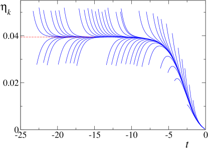
Figure 1: (color online) Example of the dichotomy procedure used for reaching the fixed point ($N=1$, $d=3$, $\tilde{u}=6\times 10^{-2},\tilde{\rho}_{0}=0,\tilde{p}_{0}=0$, $\alpha=2.25$). The plot shows the running anomalous dimension $\eta_{k}$ as a function of $t=\ln(k/\Lambda)$. Each curve corresponds to a different initial value of $r$ (see Eq.(39)). The red dashed line indicates the estimated asymptotic value $\eta\simeq 0.03943$.

V Results at criticality

Although the main goal of the BMW method is to provide access to full-momentum dependence, it can of course also be used to compute critical exponents and other zero-momentum quantities Benitez09 . In this section, where we return to the $O(N)$ models (with general $N$), we provide details on the calculation of the critical exponents and check their robustness with respect to variations of the different parameters of the method such as the numerical resolution, the choice of the cut-off function and the location of the normalization point ($\tilde{\rho}_{0}$,$\tilde{p}_{0}$).

Since we focus here on the regime of small momenta, it is convenient to take as initial condition a value of the dimensionless coupling $\tilde{u}$ not too small compared to 1 in order to initialize the flow far from the Gaussian fixed point $\tilde{u}=0$ and thus to approach quickly the infrared fixed point. This is useful, not only because of the shortened time needed to reach the critical regime, but also because otherwise, due to the 16-digit precision used, our dichotomy procedure does not allow for an accurate determination of the fixed point directly from initial parameters. The results to be presented below have been calculated for $\tilde{u}=6\times 10^{-2}/N$.

V.1 Numerical extraction of critical exponents

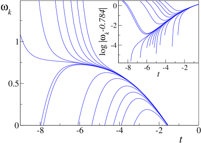
Figure 2: (color online) Running exponent $\omega_{k}$ ($d=3$, $N=1$, $\alpha=2.25$, $p_{0}=0$ and $\rho_{0}=0$). Each curve corresponds to a different initial value of $r$ (see Eq.(39)). Inset: the exponential approach to the asymptotic exponent is used to estimate $\omega\simeq 0.784$.

The anomalous dimension $\eta$ comes out of the solution of the flow equations, which provide a direct estimate of $\eta_{k}$ (Fig. 1). It can also be extracted from $\Gamma_{k=0}^{(2)}(p,\rho=0)\propto p^{2-\eta}$ at small momentum with the same result, although this is a much less practical way.

In the vicinity of the fixed point, the behavior of any dimensionless and renormalized quantity, such as the dimensionless mass, is as follows (recall that $t=\ln k/\Lambda<0$)

$$\tilde{m}_{k}^{2}=\tilde{m}^{2}_{*}+\tilde{m}_{1}^{2}{\rm e}^{-\frac{t}{\nu}}+\tilde{m}_{2}{\rm e}^{\omega t}+\tilde{m}_{3}{\rm e}^{\omega_{2}t}+\dots$$ (40)

with the universal critical exponent $\nu$ describing the departure from the critical surface, and the correction to scaling exponents $\omega,\omega_{2},\ldots$ describing the initial approach to the fixed point.

In practice, we use the flow of the mass (the flow of $\eta_{k}$ could also be used) to extract $\nu$ and $\omega$ ref20 . We explore successively regions of $t$-values where one of the exponentials in the equation above dominates. For instance, for $t$ negative enough, we write:

$$\log|\partial_{t}\tilde{m}^{2}|\sim-\frac{t}{\nu}+{\rm constant}$$ (41)

to find $\nu$. To extract $\omega$, we choose $|t|$ large enough but not so large as to leave the vicinity of the fixed point. We then write

$$\log|\partial_{t}\tilde{m}^{2}|\sim\omega t+{\rm constant}.$$ (42)

Notice that away from the fixed point, the exponents thus determined depend themselves weakly on $t$ since, strictly speaking, (40) holds only in the infinitesimal vicinity of the fixed point. We thus obtain only (slowly) running exponents $\nu_{k}$ and $\omega_{k}$. In practice, these exponents are calculated by taking the $t$-derivative of Eqs.(41,42). The procedure is then repeated for a set of initial conditions that bring the system closer and closer to the critical point. The estimates of $\nu_{k}$ and $\omega_{k}$ saturate to their fixed point values reflected in the plateau seen in Fig. 2 for $\omega_{k}$ ($\omega$ is the most difficult exponent to determine numerically). Given such curves, one can further extract even more accurate estimates from the (exponential) approach to the asymptotic plateau values, see inset of Fig. 2.

With this method we could, in principle, extract exponents with almost arbitrary numerical accuracy. In practice, however, only a few digits are significant: our results suffer indeed from an uncertainty related to the choice of the cut-off function (see next subsection); besides, it is not necessary to present results with an accuracy that far exceeds the deviation from those with which they are compared.

V.2 Dependence on renormalization point and regulator

Although as explained above the values of the critical exponents should in principle depend neither on the normalization point $(\tilde{p}_{0},\tilde{\rho}_{0})$ nor on the shape of the cut-off function $R_{k}(q)$ this is no longer the case once approximations are performed.

In practice, we apply the “principle of minimal sensitivity”, searching for a local extremum of the physical quantities under study Stevenson ; Canet03 in a “reasonable” subspace of values taken by $\alpha$ (the parameter of our cut-off function (38)), $\tilde{p}_{0}$, and $\tilde{\rho}_{0}$. It is then expected that the corresponding values are “optimal” in the sense that they show, locally, the weakest dependence on the above parameters.

Here, we first notice that at fixed $\alpha$ and $\tilde{\rho}_{0}$, the dependence of our estimates on $\tilde{p}_{0}$ is much weaker than that found by varying $\alpha$ and $\tilde{\rho}_{0}$. Fig.3 shows the variation of the anomalous dimension $\eta$ with $\alpha$ for two typical values of $N$ in three dimensions. As in all other cases studied, we observe the existence of a unique extremum. In the following, we always use these extremum values to report our best estimates for the critical exponents. Note that we do not show the variations of the exponents with $\tilde{\rho}_{0}$ as they can be shown to be equivalent to those with $\alpha$ TBP .

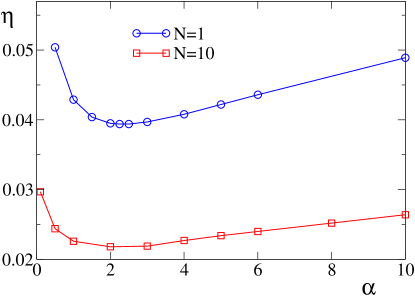
Figure 3: (color online) $\eta$ as a function of the cut-off parameter $\alpha$, for $N=1$ and $N=10$ ($d=3$, $\tilde{\rho}_{0}=0,\tilde{p}_{0}=0$).

V.3 Results for the critical exponents

We now present our results for the critical exponents of the scalar $O(N)$ models in $d=3$. They have been obtained with a two-dimensional grid in $\tilde{\rho}$ and $\tilde{q}$ with $n_{\rho}=51$ points in the $\tilde{\rho}$-direction, $n_{q}=60$ points in $\tilde{q}$ and with $\tilde{q}_{max}=4$, $\tilde{p}_{max}=6$, and a $\tilde{\rho}_{max}=5N$. Tables 1, 2 and 3 contain our results for the critical exponents $\eta$, $\nu$ and $\omega$, together with some of the best estimates available in the literature, obtained either from Monte Carlo or resummed perturbative calculations (that we refer to as field theory (FT)). Our numbers are all given for the optimal values $\alpha^{*}$ of the cut-off parameter, and the digits quoted remain stable when $\alpha$ varies in the range $[\alpha^{*}-{1}/{2},\alpha^{*}+{1}/{2}]$. The quality of these numbers is obvious: our results for $\nu$ agree with previous estimates to within less than a percent, for all $N$; as for the values of $\eta$ and $\omega$, they are typically at the same distance from the Monte-Carlo and high temperature series estimates (for instance, for $N=1$, $\nu=0.6298(3)$ arisue2004 ) as the results from resummed perturbative calculations. Our numbers also compare favorably with those obtained at order $\nabla^{2}$ in the DE scheme Canet03 .

Table 1: Results for the anomalous dimension $\eta$ in $d=3$, compared with results obtained within the DE at order $O(\nabla^{2})$, field theory (FT) and Monte Carlo (MC) methods

$N$	BMW	DE	FT	MC
0	0.034	0.039Gersdorff00	0.0272(3)Suslov08	0.0303(3))grassberger
1	0.039	0.0443Canet03	0.0318(3) Suslov08	0.03627(10) hasenbusch10
2	0.041	0.049Gersdorff00	0.0334(2) Suslov08	0.0381(2)Campostrini06
3	0.040	0.049Gersdorff00	0.0333(3) Suslov08	0.0375(5)Campostrini01
4	0.038	0.047Gersdorff00	0.0350(45) Guida98	0.0365(10)Hasenbusch01
10	0.022	0.028Gersdorff00	0.024 Antonenko98	-
100	0.0023	0.0030Gersdorff00	0.0027 Moshe03	-
$\mathcal{O}(1/N)$	$0.23/N$		$0.270/N$ Moshe03	-

Table 2: Results for the critical exponent $\nu$ in $d=3$, compared with results obtained within the DE at order $O(\nabla^{2})$, field theory (FT) and Monte Carlo (MC) methods

$N$	BMW	DE	FT	MC
0	0.589	0.590Gersdorff00	0.5886(3) Suslov08	0.5872(5) Pelisseto07
1	0.632	0.6307Canet03	0.6306(5) Suslov08	0.63002(10) hasenbusch10
2	0.674	0.666Gersdorff00	0.6700(6) Suslov08	0.6717(1) Campostrini06
3	0.715	0.704Gersdorff00	0.7060(7) Suslov08	0.7112(5)Campostrini01
4	0.754	0.739Gersdorff00	0.741(6)Guida98	0.749(2)Hasenbusch01
10	0.889	0.881Gersdorff00	0.859 Antonenko98	-
100	0.990	0.990 Gersdorff00	0.989Moshe03	-
$\mathcal{O}(1/N)$	$1-1.034/N$		$1-1.081/N$ Moshe03	-

Table 3: Results for the correction to scaling exponent $\omega$ in $d=3$ compared with results obtained within the BMW method, field theory (FT) and Monte Carlo (MC) results

$N$	BMW	FT	MC
0	0.83	0.794(6) Suslov08	0.88 grassberger
1	0.78	0.788(3) Suslov08	0.832(6) hasenbusch10
2	0.75	0.780(10) Suslov08	0.785(20) Campostrini06
3	0.73	0.780(20) Suslov08	0.773 Campostrini01
4	0.72	0.774(20) Guida98	0.765 Hasenbusch01
10	0.80	-	-
100	1.00	-	-

In the limit of large $N$, the BMW scheme becomes exact for the 2-point function for $s\geq 2$ Blaizot:2005xy ; Blaizot:2005wd . This generalizes the fact, shown in D'Attanasio97 , that the LPA ($s=0$) is exact in the large $N$ limit for the effective potential. It can be verified from the tables 1 to 4 that the large $N$ limit values $\eta=0$, $\nu=1$ and $\omega=1$ are approached for large values of $N$.

We can also perform a $1/N$ expansion ZINN ; Moshe03 . This was already done in BMWnum , where the BMW scheme was further approximated by the use of LPA propagators. As the LPA becomes exact in the large $N$ limit, these results are unchanged at first order in $1/N$, except for the use of another type of regulator profile. An analytical study of the BMW equations in this limit provides the following values for the critical exponents at order $1/N$: $\eta={0.23}/{N}$ and $\nu=1-{1.034}/{N}$, to be compared with the exact results Moshe03 $\eta={0.27}/{N}$ and $\nu=1-1.081/N$. In BMWnum the use of another regulator profile allowed us to obtain somewhat better results for $\eta$ in this limit: $\eta={0.25}/{N}$. Notice that all these analytical results are recovered in our numerical solution for large values of $N$ (notice in fact that terms of order $1/N^{2}$ are very small already for $N>4$).

The two-dimensional case, for which exact results exist, provides a very stringent test of the BMW scheme. We focus here on the Ising model $N=1$ which exhibits a standard critical behavior in $d=2$, and the corresponding critical exponents. Notice that the perturbative method that works well in $d=3$ fails here: for instance, the fixed-dimension expansion that provides the best results in $d=3$ yields, in $d=2$ and at five loops, $\eta=0.145(14)$ pogorelov07 in contradiction with the exact value $\eta={1}/{4}$. We find instead $\eta=0.254$, $\nu=1.00$ in excellent agreement with the exact values $\eta={1}/{4}$, $\nu=1$. A more detailed study of $O(N)$ models in $d=2$, at and out of criticality, will be presented in a separate work.

V.4 The function $\Gamma^{(2)}$ at criticality and further tests at intermediate and large momenta

We now study the momentum dependence of the two-point function at criticality. In dimension three, the bare coupling constant $u$ has the dimension of a momentum and thus sets a scale (the Ginzburg length: $\xi_{G}\sim u^{\frac{1}{d-4}}$). There are typically three momentum domains for $\Gamma^{(2)}(p,\rho=0)$ BMWnum ; Benitez09 :

(i) the infrared domain defined by $p\ll u$ where $\Gamma^{(2)}(p)\sim u^{\eta}p^{2-\eta}$. We show in Fig. 4 that this behavior is well reproduced by our solution of the flow equation. To clearly see this regime on a large range of momentum we have integrated the flow with a bare value of $u$ not too far from the value of $\Lambda$: $\tilde{u}=6.10^{-2}/N$.

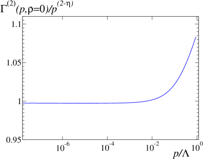
Figure 4: (color online) The ratio of the 2-point function $\Gamma^{(2)}(p,0)$ and of $p^{2-\eta}$ at criticality as a function of $p/\Lambda$ ($d=3,N=2,\alpha=2,p_{0}=0,\rho_{0}=0$). The normalization has been chosen so that this ratio starts close to 1 at small $p$. The bare dimensionless coupling is $\tilde{u}=6.10^{-2}/N$.

(ii) the ultra-violet domain defined by $p\gg u$ (and $\Lambda\gg p$) where $\Gamma^{(2)}(p)$ can be studied perturbatively and is found to behave at two loops as $\Gamma^{(2)}(p)-p^{2}\sim-(\mathcal{C}_{N}/{96\pi^{2}})u^{2}\log p/u$ (with $\mathcal{C}_{N}=(N+2)/3$). It was shown in BMWnum that in the BMW approximation, and at large momenta $\Delta(p,\rho=0)$ behaves as $u^{2}\ln(p/u)$, more precisely,

$$\frac{\partial\Delta_{k=0}(p,0)}{\partial|p|}=\mathcal{C}_{N}\frac{u^{2}}{2|p|}\int_{l,q}\partial_{t}R_{k}(l)G_{0}^{2}(l)G^{2}_{0}(q).$$ (43)

The $u^{2}\log p/u$ behavior is thus retrieved, see Fig.5, with a prefactor that however depends on $R_{k}(q)$. With the exponential cut-off function, Eq.(38), the prefactor can only be calculated numerically. We have studied its dependence on $\alpha$ and shown that there is an extremum around $\alpha\sim 5$ where the difference with the exact result is about 8$\%$. Of course, this UV behavior shows up only if the bare coupling $u$ is sufficiently small compared to $\Lambda$. We have chosen $\tilde{u}=10^{-6}/N$ to have a large UV domain where this behavior is clearly seen. Note that at small $p$, $\Gamma^{(2)}(p)-p^{2}\sim p^{2-\eta}$ which is visible on Fig.5 although this regime is approached very slowly.

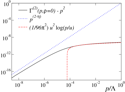
Figure 5: (color online) The difference $\Gamma^{(2)}(p,0)-p^{2}$ at criticality as a function of $p/\Lambda$, compared with its expected ultra-violet behavior $\sim u^{2}\log p/u$ ($d=3,N=2,\alpha=2,p_{0}=0,\rho_{0}=0$). The infrared $p^{2-\eta}$ behavior is also shown (see text). The bare dimensionless coupling is $\tilde{u}=10^{-6}/N$.

(iii) the cross-over between the infrared and ultra-violet domains. This regime of momentum is visible on both figures 4 and 5 for $p\simeq u$.

Table 4: Results for the quantity $c$ defined in the text.

$N$	BMW	lattice	$7$ loops Kastening03
1	1.15	1.09(9)Sun02	1.07(10)
2	1.37	1.32(2) Arnold01	1.27(10)
		1.29(5)Kashurnikov01
3	1.50		1.43(11)
4	1.63	1.60(10)Sun02	1.54(11)
10	2.02
100	2.36

For purposes of probing the intermediate momentum region between the IR and the UV, we have calculated the quantity

$$c=-\frac{256}{uN}\zeta[{3}/{2}]^{-\frac{4}{3}}\,\!\int\!{\rm d}^{3}p\left(\frac{1}{\Gamma^{(2)}(p)}\!-\!\frac{1}{p^{2}}\right)$$ (44)

which is very sensitive to the cross-over regime: the integrand in Eq. (44) is peaked at $p\sim(Nu)/10$ Blaizot04 . For this reason, the calculation of $c$ has been used as a benchmark for non-perturbative approximations in the $O(N)$ model.

In the $O(2)$ case and for $d=3$, this quantity determines the shift of the critical temperature of the weakly repulsive Bose gas Baym99 (notice that $c$ is not defined for $d=2$). It has thus been much studied recently using various methods, even for other values of $N$. In particular, the large $N$ limit for this quantity has been calculated analytically and found to be $c=2.3$ Baym00 . In this work, we have found the values for $c$ for some representative values of $N$. Our results, compared to the best ones available in the literature (with their corresponding errors when available), are presented in Table 4. For all values of $N$ where lattice and/or 7-loops resummed calculations exist, our results are within the error bars of those calculations (and comparable to those obtained from an approximation specifically designed for this quantity Blaizot:2005wd ; ref41 ), except for $N=2$, where very precise lattice results are available. In the large $N$ limit, one can see that our results differs from the exact value by less than 3%. Notice that the large $N$ behavior of the quantity $c$ is in fact of order $1/N$ Baym00 , which as we have seen is not calculated exactly at this level of the BMW approximation.

Altogether, we can see that the BMW method is able to reproduce the correct behavior of the 2-point function at criticality in all momentum regimes. Note in particular that this is not the case of conformal field theoretical methods that are only able to capture at criticality the conformally invariant $p^{2-\eta}$ behavior but that can reproduce neither the ultra-violet behavior, corresponding to $u\ll p\ll\Lambda$, nor the cross-over between the infrared and ultra-violet regions, corresponding to $p\simeq u$.

VI Scaling functions

As an approximation of the NPRG, the BMW scheme allows us to investigate all momentum, temperature and external magnetic field regimes, and is not restricted to the long distance physics at criticality. A particularly interesting, and a priori difficult regime is the critical domain, where the correlation length is large but finite. In this case, an appropriately rescaled two-point function shows a universal behavior. As the BMW approximation allows for the calculation of genuine momentum-dependent quantities, the calculation of this scaling function and its comparison with the best available theoretical results from the literature and with experimental data represent one of the most stringent tests of the approximation.

In this work, we consider the case $N=1$ relevant, for instance, to describe the critical behavior of fluids near the liquid-gas critical point. Near this point and for $p\ll\xi_{G}^{-1}\sim u$ one expects the general scaling behavior

$$G^{(2)}_{\pm}(p)=\chi g_{\pm}(p\xi)$$ (45)

with, by definition, $G^{(2)}$ the density-density correlation function, $\chi^{-1}=\Gamma^{(2)}(p=0)$ the compressibility and $\xi^{-2}=k^{2}\tilde{m}^{2}_{k},$ with $k\to 0$, the correlation length that diverges close to criticality with the $\nu$ critical exponent. Here $\pm$ refers to the two phases, above and below the critical temperature respectively. The functions $g_{\pm}(x)$, normalized so that

$$g^{-1}(x)=1+x^{2}+O(x^{4}),$$ (46)

are universal. Their limiting behavior is well known. For small $x$ they are well described by the Ornstein-Zernicke (mean-field) approximation:

$$g_{OZ}(x)=\frac{1}{1+x^{2}}.$$ (47)

The corrections to the Ornstein-Zernicke behavior are usually parameterized as martin-mayor02

$$g_{\pm}(x)^{-1}=1+x^{2}+\sum_{n=2}c_{n}^{\pm}x^{2n}\;.$$ (48)

The above behavior of $g_{\pm}(x)^{-1}$ is a priori valid only for $x<1$ but since the coefficients $c_{n}$ are very small, it turns out that the Ornstein-Zernicke approximation is actually valid over a wide range of $x$ values, as we shall see later. For large $x$ (that is, $\xi\gg p^{-1}$) the scaling functions show critical behavior with an anomalous power law decay

$$g_{\pm}(x)=\frac{C_{1}^{\pm}}{x^{2-\eta}},$$ (49)

which allows for the experimental determination of the exponent $\eta$. This expression also allows for corrections, as given by Fischer and Langer fisher68

$$g_{\pm}(x)=\frac{C_{1}^{\pm}}{x^{2-\eta}}\bigg{(}1+\frac{C_{2}^{\pm}}{x^{(1-\alpha)/\nu}}+\frac{C_{3}^{\pm}}{x^{1/\nu}}+\dots\bigg{)}.$$ (50)

Different approximate results for the universal scaling functions exist in the literature, obtained either by Monte Carlo methods martin-mayor02 , or by the use of an analytical ansatz, interpolating between the two know limiting regimes (48) and (49), using $\varepsilon$ expansion results (the Bray approximation bray76 ). Experimental results from neutron scattering in ${\rm CO}_{2}$ near the critical point also exist damay98 .

In Bray’s interpolation for the high temperature phase one assumes $g^{-1}_{+}(x)$ to be well defined in the complex $x^{2}$ plane, with a branch cut in the negative real $x^{2}$ axis, starting at $x^{2}=-r^{2}_{+}$, where $r_{+}^{2}=9M_{\rm gap}^{2}\xi^{2}\equiv 9S_{M}$, following the theoretical expectation that the singularity of $g_{+}(x)$ nearest to the origin is the three-particle cut ferrell75 ; bray76 . The parameter $M_{\rm gap}$ is the mass gap of the Minkowskian version of the model. For the $\phi^{4}$ theory, it is known that the difference between the mass gap and $\xi^{-1}$ is very small and replacing one by the other corresponds to an error which is beyond the accuracy of our calculation martin-mayor02 . Then Bray’s ansatz in the high temperature phase (the only phase studied in the following) reads:

$$g^{-1}_{+}(x)= \frac{2\sin\pi\eta/2}{\pi C_{1}^{+}}$$ (51)

$$\times\int_{r+}^{\infty}du\;F_{+}(u)\bigg{[}\frac{S_{M}}{u^{2}-S_{M}}+\frac{x^{2}}{u^{2}+x^{2}}\bigg{]}$$

where $F_{+}(u)$ is the spectral function, which satisfies $F_{+}(+\infty)=1$, $F_{+}(u)=0$ for $u<r_{+}$, and $F_{+}(u)\geq 0$ for $u\geq r_{+}$. On top of this, one must impose $g^{-1}(0)=1$, which fixes the value for $C_{1}^{+}$.

One must then specify $F_{+}(u)$. Bray bray76 proposed the use of a spectral function with the exact Fischer-Langer asymptotic behavior, of the type

$$F_{+,B}(u)=\frac{P_{+}(u)-Q_{+}(u)\cot\frac{1}{2}\pi\eta}{P_{+}(u)^{2}+Q_{+}(u)^{2}}$$ (52)

where

$$P_{+}(u) =1+\frac{C_{2}^{+}}{u^{\iota}}\cos\frac{\pi\zeta}{2}+\frac{C_{3}^{+}}{u^{1/\nu}}\cos\frac{\pi}{2\nu}$$

$$Q_{+}(u) =\frac{C_{2}^{+}}{u^{\iota}}\sin\frac{\pi\zeta}{2}+\frac{C_{3}^{+}}{u^{1/\nu}}\sin\frac{\pi}{2\nu}$$ (53)

with $\zeta\equiv(1-\alpha)/\nu$. This definition contains a certain number of parameters. On top of the critical exponents, which can be injected using either the BMW values or the best available results in the literature, one must also fix $S_{M}^{+}$, $C_{2}^{+}$ and $C_{3}^{+}$. For $S_{M}^{+}$ one can use the best estimate in the literature, given by the high temperature expansion of improved models Campostrini02b . Bray proposed to fix $C_{2}^{+}+C_{3}^{+}$ to its $\varepsilon$-expansion value $C_{2}^{+}+C_{3}^{+}=-0.9$, and to then determine $C_{1}^{+}$ by requiring $F_{+,B}(r_{+})=0$. These conditons allows for a little parameter tuning, by adjusting the relative weight of the $C_{2}^{+}$ and $C_{3}^{+}$ parameters. When comparing our results with Bray’s ansatz, we shall use this freedom. We now turn to the scaling function computed by the BMW method.

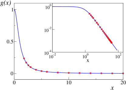
Figure 6: (color online) The 2-point scaling function $g(p\xi)$ as a function of $x=p\xi$ in the high-temperature phase ($d=3$, $N=1$). Solid blue line: BMW result. Red squares: Experimental results of damay98 . Inset: same data with logarithmic scales.

In terms of the variables used in this paper, we find that

$$g^{-1}(p\xi)=\frac{(p\xi)^{2}+\Delta(p\xi,0)+Z_{k}k^{2}m^{2}_{k}(0)}{Z_{k}k^{2}m^{2}_{k}(0)}$$ (54)

when $k\to 0$. In this work, for purposes of comparison with existing results, we have only computed the high temperature scaling function. We have performed the calculation for different values of the correlation length (and hence of the reduced temperature). When plotted, one can indeed see perfect data collapse for different values of $\xi$, which is the first non trivial test of the quality of our results for the scaling function.

In Fig.6 we plot the BMW scaling function together with the experimental results from reference damay98 . Due to the small values taken by the coefficients $c_{n}$ and the critical exponent $\eta$ in $d=3$, the Ornstein-Zernicke behavior dominates even beyond $p\xi=1$. In order to measure the deviation from this behavior, one usually makes use of the auxiliary function

$$h(x)=\log\bigg{[}\frac{g(x)}{g_{OZ}(x)}\bigg{]}.$$ (55)

In Fig.7 we plot this function together with the experimental results from damay98 and the results from the Bray ansatz for two “extreme” choices of the $C_{2}^{+}$ and $C_{3}^{+}$ parameters. One can there see that the BMW approximated result compares very well with all these results. In particular, it is in between the results obtained from the two Bray ansatz considered.

Let us mention that even with large system sizes, the Monte Carlo results suffer from significant systematic errors for $p\xi$ larger than typically 5 to 10. This probably comes from the fact that the universal behavior of the structure factor shows up only when $\xi$ and the separation $l$ between the spins at which we calculate the correlation function are large compared to the lattice spacing and small compared to the lattice size: even for lattice sizes of a few hundreds of lattice spacings this leaves only a small window of useful values of $\xi/l$ martin-mayor02 .

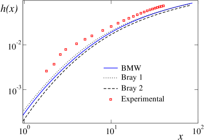
Figure 7: (color online) Deviation of the scaling function to its trivial Ornstein-Zernicke form, Eq.(55). The dotted and dashed lines correspond to two “extreme” choices of the parameters $C_{2}$ and $C_{3}$ of Bray’s ansatz. Dotted line: $C_{1}=0.924$, $C_{2}=1.8$, $C_{3}=-2.28$. Dashed line: $C_{1}=0.918$, $C_{2}=2.55$, $C_{3}=-3.45$.

On top of these results we can also compare results for the values of the coefficients $c_{2}^{+}$ and $C_{1}^{+}$. The results for BMW are $c_{2}^{+}\sim-4.5\times 10^{-4}$ to be compared with the IHT best estimate Campostrini02b $c_{2}^{+}=-3.90(6)\times 10^{-4}$, whereas for $C_{1}^{+}$ BMW yields $C_{1}^{+}=0.914$, to be compared with the $\varepsilon$-expansion result $C_{1}^{+}=0.92$.

We conclude this section by noting that (i) the structure factor encompasses much more informations on the universal behavior of a model than the (leading) critical exponents (that are moreover difficult to measure experimentally), (ii) Bray’s ansatz, although powerful, depends on two parameters $C_{2}$ and $C_{3}$ that are poorly determined perturbatively as well as on two critical exponents, (iii) the present state of the art of the Monte Carlo simulations is by far insufficient to compute reliably the structure factor in the interesting region of momentum where $p\xi$ is large, (iv) the BMW method leads to a determination of the structure factor that has no free parameter once a choice of regulator has been made (possibly involving an optimization procedure as described in Section V.2). The results above, summarized in Fig.7, suggest that the BMW method leads to an accurate determination of the structure factor in the whole momentum range while the experimental results seem to suffer at small momentum from systematic deviations.

VII Relation with the derivative expansion

The validity of the DE is rarely questioned, satisfactory results being taken as an a posteriori check. We show now that the BMW approach allows for a deeper understanding of its range of applicability, and of some of its peculiar features.

The ansatz defining the order of the DE (see, for instance, Eq.(12) for the order 2) is used to

(i) define the quantities to be determined, which, in the case of order 2, are the effective potential and the field normalization, both functions of the (constant) field $\phi$

$$\left\{\begin{array}[]{l}\displaystyle{V_{k}(\phi)=\frac{1}{\Omega}{\Gamma_{k}[\phi(x)]}{\big{|}_{\phi(x)=\phi}}}\\ \\ \displaystyle{Z_{k}(\phi)=\partial_{p^{2}}\left(\Gamma_{k}^{(2)}[p,\phi]\right){\big{|}_{p=0,\phi}}}\,.\end{array}\right.$$ (56)

(ii) compute the $n$-point functions $\Gamma_{k}^{(n)}$ and the propagator $G_{k}=(\Gamma_{k}^{(2)}+R_{k})^{-1}$ that enter the right hand sides of the flow equations of $V_{k}$, $Z_{k}$, etc.

In short, the DE projects the functional $\Gamma_{k}[\phi]$ on a polynomial expansion in powers of the derivatives of the field, the expansion coefficients being field dependent. In Fourier space, the DE amounts to a polynomial expansion of the $n$-point functions $\Gamma_{k}^{(n)}(p_{1},\cdots,p_{n},\phi)$ in powers of the momenta $p_{i}$, around vanishing momenta (see for instance Eq. (18)). At this point, it is useful to introduce a distinction between external momenta, the momenta that appear in the $n$-point function $\Gamma_{k}^{(n)}(p_{1},\cdots,p_{n},\phi)$ whose flow is being considered, and the internal momentum, denoted by $q$, appearing in the $n$-point functions in the r.h.s. of the corresponding flow equation and which is integrated over. In contrast to what is done in the BMW approximation, in the DE no distinction is made between these two sets of momenta, which can lead to inconsistencies. For instance, in the flow equation for $Z_{k}(\phi)$ at order 2, the product $\Gamma_{k}^{(3)}(p,q,-p-q)\Gamma_{k}^{(3)}(-p,-q,p+q)$ (see Eq.(11)) leads to four terms of order four: $(p^{2})^{2},p^{2}q^{2},(p.q)^{2},(q^{2})^{2}$, that, in a strict expansion to this order, should be neglected (note that this is not what is usually done in the DE context). In fact, since $Z_{k}(\phi)$ is already the coefficient of the $p^{2}$ term in the expansion of $\Gamma_{k}^{(2)}(p,\phi)$, any dependence of $\Gamma_{k}^{(3)}$ (and of $\Gamma_{k}^{(4)}$) on the internal momentum $q$ should be neglected in $\partial_{k}Z_{k}(\phi)$ at this order of the DE. Since the BMW approximation at order $s=2$ precisely consists in setting $q=0$ in $\Gamma_{k}^{(3)}$ and $\Gamma_{k}^{(4)}$ in the flow equation of $\Gamma_{k}^{(2)}$, we conclude that at this order the BMW approximation contains all terms of the DE at order $\nabla^{2}$.

The BMW approximation, that disentangles the roles of the internal and external momenta, differs deeply from the DE precisely on the point explained above: as the DE, it takes advantage of the fact that the internal momentum is cut-off by $\partial_{k}R_{k}(q)$ in order to expand in powers of $q/k$ (in fact only the leading term, $q=0$, is retained), but does not rely on the smallness of the external momenta.

In fact, the natural expansion parameter of the DE is the ratio $p/k$ or $p/m$, whichever is smallest, where $m$ is the smallest of the masses that may appear in the problem considered: When $k$ is much larger that all masses, these can be ignored and $p/k$ is the expansion parameter. When $k$ becomes smaller that the smallest mass, the flow essentially stops and the expansion parameter becomes $p/m$ in the limit $k\to 0$. Thus, it is plausible that the DE performed as a power series in $p/k$ in a critical theory ($m=0$) possesses a radius of convergence of the same order as the DE performed as a power series in $p/m$ in a massive theory at $k=0$. In this last case, the radius of convergence is known for $N=1$ in dimension three (ferrell75 ; bray76 ): It is 3 in the symmetric phase and 2 in the broken phase .

The above arguments suggest that the DE is not able to describe $k$-dependent correlation functions with external momenta higher than typically $3\,\mathrm{max}(k,m)$. In particular, in the critical case where massless modes are present, the DE is only suited for the calculation of physical (that is at $k=0$) correlation functions at $p=0$: The anomalous momentum behaviour $\Gamma_{k=0}^{(2)}(p)\sim p^{2-\eta}$, valid at small $p$, will not emerge at any order of the DE. Of course, this does not mean that the anomalous dimension cannot be determined within the DE, as one can exploit general scaling relations and the fact that the anomalous dimension enters also quantities that are defined at zero momentum. Thus, for instance, $\eta$ can be estimated from the $k$-dependence of the normalization factor $Z_{k}\sim k^{-\eta}$ (or alternatively from the large field behavior of the fixed-point dimensionless effective potential). In contrast, the BMW approximation correctly captures the anomalous scaling of $\Gamma_{k=0}^{(2)}(p)$ at small $p$, and this is a direct consequence of the fact that no expansion in external momenta is performed.

The origin of the difficulties of the DE is that it does not have good decoupling properties in the momentum range $p\gg k$. The decoupling property, crucial for universality, means, on the example on the 2-point function, that $\Gamma_{k}^{(2)}(p)$ becomes almost $k$-independent when $k\ll p$ and that therefore $\Gamma_{k=0}^{(2)}(p)\simeq\Gamma_{k=p}^{(2)}(p)$. One could thus naively expect that external momenta $\{p_{i}\}$, $i=1,\dots,n$ play the role of infrared regulators in the flow of $\Gamma_{k}^{(n)}(\{p_{i}\})$ and that when $k<p_{i},\forall i$ the flow of $\Gamma_{k}^{(n)}$ (almost) stops. In fact, in flow equations, external momenta play, at best, the role of infrared regulators when all momenta involved (external and internal) are not in an exceptional configuration. The problem is that even when the external momenta are not exceptional, the integral over the internal momentum $q$ in the flow equation of $\Gamma_{k}^{(n)}$ involves vertex functions ($\Gamma_{k}^{(n+1)}$ or $\Gamma_{k}^{(n+2)}$) in exceptional configurations. Depending on the approximation scheme, this can spoil the decoupling property that, undoubtly, should hold for the (physical, that is $k\ll p$) correlation functions themselves when they are evaluated in non-exceptional configurations. The difficulty is therefore to devise an approximation scheme that satisfies the decoupling property. While this is the case of the BMW scheme it is neither of perturbation theory nor of the DE. One can nevertheless try to extract from the DE the gross behavior of $\Gamma^{(2)}(p)$ (and of the other functions) by stopping by hand the flow at $k=p$ and identifying $\Gamma_{k=p}^{(2)}(p)$ with $\Gamma_{k=0}^{(2)}(p)$. This idea has been explored in Blaizot:2005wd (see also Dupuis2009 ). The resulting correlation functions roughly show the expected momentum behavior, but as analyzed in detail in Blaizot:2005wd , it does not seem possible to extend this first qualitative analysis and to obtain quantitatively precise correlation functions without having recourse to BMW.

To gain further insight into the validity of the DE, we may consider a simple analytical representation of the function $\Gamma_{k=0}^{(2)}(p,\phi)$ determined with the BMW approximation at order $s=2$, which, as we have shown, is very close to the exact 2-point function over the whole momentum range. The following formula (inspired by Eq.(2.33) of Berges02 )

$$\begin{array}[]{ll}\Gamma_{k}^{(2)}(p,\rho)=&Ap^{2}\left(p^{2}+b\,k^{2}+b^{\prime}\,M^{2}_{k}(\rho)\right)^{-\eta_{k}/2}\\ &+V_{k}^{\prime}+2\rho V_{k}^{\prime\prime}\end{array}$$ (57)

where $A$, $b$, and $b^{\prime}$ are independent of $p$ and $\rho$, and $M^{2}_{k}(\rho)$ is a function homogeneous to a square mass, provides a good fit of the BMW results when $k$, as well as $M^{2}_{k}(\rho)$, are very small compared to the ultra-violet cut-off $\Lambda$. This formula encompasses the two different regimes that characterize the behavior of $\Gamma_{k}^{(2)}(p)$ at small $p$: First, for $p$ small compared to $\Lambda$ and large compared to $k$ and to the mass, it yields $\Gamma_{k}^{(2)}(p)\sim p^{2-\eta_{k}}$, with $\eta_{k}$ the running anomalous dimension. Thus, the critical behavior is captured for $k$ sufficiently small for $\eta_{k}$ to be quasi-stationary and (almost) equal to $\eta$. Second, for $p$ small compared to either $M_{k}$ or $k$, one can expand $\Gamma_{k}^{(2)}(p,\phi)$ in powers of $p^{2}/(k^{2}+M_{k}^{2})$ and get:

$$\Gamma_{k}^{(2)}(p,\rho)=A^{\prime}\left(k^{2}+b^{\prime\prime}\,M^{2}_{k}(\rho)\right)^{-\eta_{k}/2}\\ \times p^{2}\left(1+f_{1,k}(\rho)p^{2}+f_{2,k}(\rho)p^{4}+\dots\right)\\ +V_{k}^{\prime}+2\rho V_{k}^{\prime\prime}.\ \ \ \ \ \ \ \$$ (58)

This is the kind of ansatz considered by the DE and it illustrates how the anomalous dimension can be extracted from the $k$-dependence of the coefficient of the $p^{2}$ term in the running action Blaizot:2005wd .

Finally, let us stress that the above remarks, while they provide some justification for the DE and in particular specify the conditions for its validity, are not sufficient to prove convergence, which may be strongly affected by the regulator. In particular, one may expect systematic errors in cases where the range of the cut-off function $R_{k}(q)$ is not smaller than the natural radius of convergence of the DE. Notice however that at least for $N=1$ in $d=3$, the smallness of the $c_{n}$ coefficients in Eq. (48) suggest that even at low order the DE should be able to capture the low momentum physics. An in-depth study of this issue will be presented in TBP .

VIII Conclusions

In this paper we have presented the complete numerical implementation of the BMW approximation scheme that allows for a solution of the NPRG flow equations keeping the full momentum dependence of the 2-point function. At the level considered in this paper, this amounts to solve two coupled equations for the effective potential and the 2-point function. These equations can be solved by elementary numerical techniques.

We have considered applications to the $O(N)$ models, mostly in dimension $d=3$. An accurate momentum dependence of the 2-point function has been obtained from the low momentum critical region to the high momentum, perturbative, region (such a region exists when the dimensionful bare coupling is small compared to the ultraviolet cutoff). In particular, the critical exponents are accurately determined as was already reported in Benitez09 . The additional results presented in this paper concerns the scaling functions which probe a different aspect of the momentum dependence of the 2-point function in the vicinity of the critical point. We have considered more specifically the scaling function for the case $N=1$ above the critical point and have shown that it is in excellent agreement with the best available theoretical estimates. Interestingly, these estimates, including ours, differ significantly from the experimental data at small momenta. These scaling functions, which are difficult to obtain with other more conventional techniques, including Monte Carlo simulations, come out directly from the 2-point function obtained by solving the flow equations.

Another information of physical interest which is also contained in the 2-point function that we compute is its field dependence. Thus a natural application of the present method could be the investigation of the $O(N)$ models in the presence of an external magnetic field. We could also contemplate extracting from the 2-point function information about possible bound states Caselle02 . Finally, we note that the BMW method paves the way towards understanding a variety of situations where the momentum structure plays a crucial role. For instance, a method similar in spirit has been applied successfully to the determination of the fixed point structure of the Kardar-Parisi-Zhang equation KPZPRL ; Canet11TBP and to the calculation of the spectral function in a Bose gas Dupuis2009 .

IX Acknowledgements

We thank N. Dupuis for discussions and remarks on a first version of the manuscript.

Appendix A Notation and conventions

By taking successive functional derivatives of $\Gamma_{k}[\phi]$ with respect to $\phi(x)$, and then letting the field be constant, one gets the $n$-point functions

$$\Gamma_{k}^{(n)}(x_{1},\cdots,x_{n},\phi)\equiv\left.\frac{\delta^{n}\Gamma_{k}}{\delta\phi(x_{1})\dots\delta\phi(x_{n})}\right|_{\phi(x)\equiv\phi}$$ (59)

in a constant background field $\phi$. Since the background is constant, these functions are invariant under translations of the coordinates, and it is convenient to factor out of the definition of their Fourier transform the $\delta$-function that expresses the conservation of the total momentum. Thus, with the usual abuse of notation, we define the $n$-point functions $\Gamma_{k}^{(n)}(p_{1},\dots,p_{n},\phi)$ as:

$$\hskip-14.22636pt(2\pi)^{d}\;\delta^{(d)}\Big{(}\sum_{j}p_{j}\Big{)}\;\Gamma_{k}^{(n)}(p_{1},\cdots,p_{n},\phi)\equiv\qquad\qquad$$

$$\hskip-14.22636pt\int d^{d}x_{1}\dots d^{d}x_{n}\;e^{i\sum_{j}p_{j}x_{j}}\Gamma_{k}^{(n)}(x_{1},\cdots,x_{n},\phi).$$

We use here the convention of incoming momenta, and it is understood that in $\Gamma_{k}^{(n)}(p_{1},\dots,p_{n},\phi)$ the sum of all momenta vanishes, so that $\Gamma_{k}^{(n)}$ is actually a function of $n-1$ momentum variables (and of $\phi$). Notice that we use brackets for functional, e.g. $\Gamma_{k}[\phi]$, and parenthesis for functions, e.g. $\Gamma_{k}^{(n)}(p_{1},\cdots,p_{n},\phi)$ when $\phi$ is uniform. For the 2-point function evaluated in a uniform field configuration, which effectively depends on a single momentum $p$, we often use the simplified notation $\Gamma_{k}^{(2)}(p,\phi)$ in place of $\Gamma_{k}^{(2)}(p,-p,\phi)$.

Appendix B Extension of BMW

In the approximation BMW with $s=2$, we make the following substitutions in the r.h.s. of the flow equation for $\Gamma_{k}^{(2)}(p)$: $\Gamma_{k}^{(4)}(p,-p,q,-q)\longrightarrow\Gamma_{k}^{(4)}(p,-p,0,0)$, and $\Gamma_{k}^{(3)}(p,q,-p-q)\longrightarrow\Gamma_{k}^{(3)}(p,0,-p)$, that is, we set the loop momentum $q$ to zero in the 3 and 4-point functions. (In this appendix we do not indicate explicitly the dependence on $\phi$ of all $n$-point functions in order to alleviate the notation.) By doing so, one obtains a closed equation for the 2-point function $\Gamma_{k}^{(2)}(p)$, which is the object calculated with optimum accuracy at the level $s=2$. As explained in the main part of the article, the general strategy to obtain the 3 and 4-point functions with comparable accuracy is to consider higher orders ($s>2$) in the approximation scheme. However, in this appendix we show that one can already improve the accuracy of $\Gamma_{k}^{(3)}$ and $\Gamma_{k}^{(4)}$ simply by exploiting the information available on $\Gamma_{k}^{(2)}(p)$.

Let us consider first the function $\Gamma_{k}^{(4)}$. We know that, at one-loop and in vanishing fields, it has the following structure

$$\Gamma_{k}^{(4),1\,{\rm loop}}(p_{1},p_{2},p_{3},p_{4})$$

$$=f(p_{1}+p_{2})+f(p_{1}+p_{3})+f(p_{1}+p_{4}),$$

where the function $f(p)$ is easily found to be

$$f(p)=\frac{1}{2}\Gamma_{k}^{(4)}(p,-p,0,0)-\frac{1}{6}\Gamma_{k}^{(4)}(0,0,0,0).$$

Since $\Gamma_{k}^{(4)}(p,-p,0,0)=\partial_{\phi}^{2}\Gamma_{k}^{(2)}(p)$ (for constant field $\phi$), we arrive at the following expression for the 4-point function in terms of the 2-point function $\Gamma_{k}^{(2)}(p)$:

$$\Gamma_{k}^{(4)}(p_{1},p_{2},p_{3},p_{4})\approx\frac{1}{2}\partial_{\phi}^{2}\Gamma_{k}^{(2)}(p_{1}+p_{2})$$

$$+\frac{1}{2}\partial_{\phi}^{2}\Gamma_{k}^{(2)}(p_{1}+p_{3})+\frac{1}{2}\partial_{\phi}^{2}\Gamma_{k}^{(2)}(p_{1}+p_{4})$$

$$-\frac{1}{2}\partial_{\phi}^{2}\Gamma_{k}^{(2)}(0).$$ (62)

Note that this expression is, by construction, symmetric under the exchange of the external legs, and it is 1-loop exact at zero external field.

For the function $\Gamma_{k}^{(3)}$, one can extract the following equivalent in the limit of vanishing field:

$$\frac{\Gamma_{k}^{(3)}(p,q,l)}{\phi} \sim\partial_{\phi}\Gamma_{k}^{(3)}(p,q,l)\Big{|}_{\phi=0}$$ (63)

$$\sim\Gamma_{k}^{(4)}(p,q,l,0)\Big{|}_{\phi=0}\ .$$

Then, by using the approximation above for $\Gamma_{k}^{(4)}$ (B) one obtains the following expression for $\Gamma_{k}^{(3)}$, whose zero field equivalent is exact at one-loop:

$$\Gamma_{k}^{(3)}(p,q,l)\approx\frac{1}{2}\partial_{\phi}\Gamma_{k}^{(2)}(p)+\frac{1}{2}\partial_{\phi}\Gamma_{k}^{(2)}(q)$$

$$+\frac{1}{2}\partial_{\phi}\Gamma_{k}^{(2)}(l)-\frac{1}{2}\partial_{\phi}\Gamma_{k}^{(2)}(0).$$ (64)

At this point, we note that we may use the new expressions that we have obtained for $\Gamma_{k}^{(3)}$ and $\Gamma_{k}^{(4)}$ in the flow equation for $\Gamma_{k}^{(2)}$. Since these $n$-point functions are now one-loop exact, the resulting approximation for $\Gamma_{k}^{(2)}$ will be 2-loop exact in zero external field. This yields therefore an improvement of the BMW approximation, in particular in the high momentum region where we know that it loses accuracy.

Consider then Eq. (11) for $\Gamma_{k}^{(2)}$, and re-write it in terms of $\Delta_{k}(p)$:

$$\partial_{t}\Delta_{k}(p;\rho)=\int_{q}\,\partial_{t}R_{k}(q)\,G_{k}^{2}(q)$$

$$\times\Big{\{}[\Gamma_{k}^{(3)}(p,q,-p-q)]^{2}G_{k}(q+p)$$

$$\hskip 14.22636pt-[\Gamma_{k}^{(3)}(0,q,-q)]^{2}G_{k}(q)$$

$$- \frac{1}{2}[\Gamma_{k}^{(4)}(p,-p,q,-q)-\Gamma_{k}^{(4)}(0,0,q,-q)]\Big{\}}.$$

Next, perform the substitutions (B) and

$$\Gamma_{k}^{(4)}(p,-p,q,-q) \to \frac{1}{2}\partial_{\phi}^{2}\Gamma_{k}^{(2)}(p+q,-p-q)$$ (66)

$$+\frac{1}{2}\partial_{\phi}^{2}\Gamma_{k}^{(2)}(p-q,-p+q).$$

One then gets

$$\partial_{t}\Delta_{k}(p)=2\rho H(p)-\frac{1}{2}L(p),$$ (67)

with

$$H(p)\equiv\int_{q}\,\partial_{t}R_{k}(q)\,G_{k}^{2}(q)\Big{\{}G_{k}(q+p)\big{[}\frac{1}{2}\Delta_{k}^{\prime}(p)$$

$$\ \ \ \ \ +\frac{1}{2}\Delta_{k}^{\prime}(q)+\frac{1}{2}\Delta_{k}^{\prime}(p+q)+3V_{k}^{\prime\prime}+2\rho V_{k}^{\prime\prime\prime}\big{]}^{2}$$

$$\ \ \ \ \ -G_{k}(q)\big{[}\Delta_{k}^{\prime}(q)+3V_{k}^{\prime\prime}+2\rho V_{k}^{\prime\prime\prime}\big{]}^{2}\Big{\}},$$ (68)

and

$$L(p) = \int_{q}\,\partial_{t}R_{k}(q)\,G_{k}^{2}(q)\Big{\{}\Delta_{k}^{\prime}(p+q)+$$ (69)

$$\hskip-28.45274pt2\rho\,\Delta_{k}^{\prime\prime}(p+q)-\Delta_{k}^{\prime}(q)-2\rho\,\Delta_{k}^{\prime\prime}(q)\Big{\}}.$$

It is not difficult to generalize these expressions to the $O(N)$ model with arbitrary $N$. However, we do not present these here because, in spite of the good properties presented above, this extended version of the BMW approximation proves to be numerically unstable and we have not been able to solve the corresponding equations with simple techniques. A further analysis, using more elaborate numerical techniques, is called for.

Appendix C Integrals

In this appendix, we give details on the calculation of the integrals $I_{n}(k;\rho)$ and $J_{n}(p;k;\rho)$.

In the case of the integral $I_{n}(k;\rho)$, since $G_{k}(q)$ (in a uniform external field) depends only on $q^{2}$, the angular integral is straightforward. One gets

$$I_{n}=\frac{S_{d}}{(2\pi)^{d}}\int_{0}^{\infty}dq\,q^{d-1}\,\,\partial_{t}R_{k}(q)\,\,G^{n}_{k}(q;\rho),$$

where

$$S_{d}=\frac{2\pi^{d/2}}{\Gamma(d/2)},\qquad K_{d}=\frac{S_{d}}{d(2\pi)^{d}}.$$ (71)

In the case of the integral $J_{n}(p;k;\rho)$, the presence of the external momentum $p$ makes the angular integral more involved.

C.1 Angular integrations

Consider integrals generically of the form

$$\int_{q}\,g(q)\,F(|p+q|)\equiv{\cal I}(p).$$ (72)

One can proceed as follows

$${\cal I}(p) = \int_{q}\,g(q)\,F(|p+q|)$$ (73)

$$= \int_{0}^{\infty}dq\,q^{d-1}\,g(q)\,\int\frac{d\Omega_{d}}{(2\pi)^{d}}F(|p+q|)$$

$$= \frac{S_{d-1}}{(2\pi)^{d}}\int_{0}^{\infty}dq\,q^{d-1}\,g(q)$$

$$\hskip-11.38092pt\times\int_{0}^{\pi}d\theta\sin^{d-2}\theta\,\,F(\sqrt{p^{2}+q^{2}+2pq\cos\theta})$$

$$= \frac{S_{d-1}}{(2\pi)^{d}}\int_{0}^{\infty}dq\,q^{d-2}\,\frac{g(q)}{p}$$

$$\times\int_{|p-q|}^{p+q}d\xi\,\xi\,{\cal J}_{d}(\xi,p,q)\,F(\xi),$$

where we made the change of variables $\xi\equiv\sqrt{p^{2}+q^{2}+2pq\cos\theta}$, and

$${\cal J}_{d}(\xi,p,q)\equiv\left[1-\left(\frac{\xi^{2}-p^{2}-q^{2}}{2pq}\right)^{2}\right]^{\frac{d-3}{2}}.$$ (74)

The interest of the last formula (73) lies in the fact that the needed integration points belong to the grid so that the integral can be calculated numerically without the need of interpolation. Furthermore, this method is particularly convenient in $d=3$ because the Jacobian (74) is then trivial.

C.2 Dimensions less than- 3

The Jacobian (74), is unity in $d=3$, and regular for $d>3$, but becomes singular for $d<3$. More precisely, for $d<3$ it diverges when $\xi$ approaches the boundaries of its integration domain ($\xi=p+q$ or $|p-q|$). Even if the integral eventually converges, this divergence is the source of numerical difficulties.

We then use for $d<3$ a different strategy, based on Cartesian variables. We define $q_{1}$ as the component of $q$ along $p$, and proceed as follows

$${\cal I}(p) = \int\frac{d^{d-1}q_{2}}{(2\pi)^{d-1}}\int_{-\infty}^{+\infty}\frac{dq_{1}}{2\pi}\,g(q)\,F(|p+q|)$$

$$= \frac{S_{d-1}}{(2\pi)^{d}}\int_{0}^{\infty}q_{2}^{d-2}dq_{2}$$

$$\hskip-22.76228pt\times\int_{-\infty}^{\infty}dq_{1}\,g(q)\,F\Big{(}\sqrt{p^{2}+q_{1}^{2}+q_{2}^{2}+2pq_{1}}\Big{)},$$

with $q$ the modulus of the vector ${\bf q}$: $q=\sqrt{q_{1}^{2}+q_{2}^{2}}$ and $|p+q|=\sqrt{p^{2}+q_{1}^{2}+q_{2}^{2}+2pq_{1}}$.

This expression has no singularities for $d\geq 2$ but it requires multiple interpolations that make the numerics more involved than in $d\geq 3$.

C.3 Small momentum limits

The integral $J_{n}(p;k;\rho)$ is regular when $p\to 0$. However, the expression given by the angular integration does not make this manifest. To get the small $p$ behavior of the generic integral (72), one can expand directly $F(|{\bf p+q}|)-F(q)$ in the first line of eq. (73):

$$F(|{\bf p+q}|) - F(q)=\frac{2{\bf p\cdot q}+p^{2}}{2q}\partial_{q}F(q)$$ (76)

$$+ \frac{({\bf p}\cdot{\bf q})^{2}}{2q^{2}}\left(\partial_{q}^{2}F(q)-\frac{1}{q}\partial_{q}F(q)\right)$$

$$+{\cal O}(p^{3}).$$

Then one can use, with the brackets denoting angular averages,

$$\langle f(q)\rangle = \frac{1}{S_{d}}\int d\Omega_{d}\,f(q)=f(q)$$

$$\langle({\bf q\cdot p})\,f(q)\rangle = \frac{1}{S_{d}}\int d\Omega_{d}\,({\bf q\cdot p})\,f(q)=0$$

$$\langle({\bf q\cdot p})^{2}\,f(q)\rangle = \frac{1}{S_{d}}\int d\Omega_{d}\,({\bf q\cdot p})^{2}\,f(q)$$ (77)

$$=\frac{p^{2}\,q^{2}}{d}f(q),$$

to obtain

$$\left\langle F(|{\bf p+q}|)-F(q)\right\rangle$$

$$=\frac{p^{2}}{2d}\left(\partial_{q}^{2}F(q)+\frac{d-1}{q}\partial_{q}F(q)\right)+{\cal O}(p^{4}),$$

and

$${\cal I}(p) - {\cal I}(0)$$ (79)

$$\ \ \ = \frac{p^{2}}{2}\,K_{d}\int_{0}^{\infty}dq\,g(q)\,\,q^{d-1}\,$$

$$\times\Big{(}\partial_{q}^{2}F(q)+\frac{d-1}{q}\partial_{q}F(q)\Big{)}+{\cal O}(p^{4})$$

$$\ \ \ = \frac{p^{2}}{2}\,K_{d}\int_{0}^{\infty}dq\,g(q)\,\partial_{q}\Big{(}q^{d-1}\,\partial_{q}F(q)\Big{)}$$

$$+{\cal O}(p^{4}).$$

Appendix D Generalization to $O(N)$ models

In this appendix the $s=2$ BMW approximation and the corresponding flow equations are presented for $O(N)$ models. The exact flow of the 2-point function in a constant external field reads (we omit the renormalization group parameter $k$ in this appendix for notational simplicity):

$$\partial_{t}\Gamma_{ab}^{(2)}(p,\mbox{\boldmath$\phi$})=\int_{q}\partial_{t}(R(q))_{in}\Big{\{}G_{ij}(q,\mbox{\boldmath$\phi$})$$

$$\times\Gamma_{ajh}^{(3)}(p,q,-p-q,\mbox{\boldmath$\phi$})G_{hl}(q+p,\mbox{\boldmath$\phi$})$$

$$\times\Gamma_{blm}^{(3)}(-p,p+q,-q,\mbox{\boldmath$\phi$})G_{mn}(q,\mbox{\boldmath$\phi$})$$

$$-\frac{1}{2}G_{ij}(q,\mbox{\boldmath$\phi$})\Gamma_{abjh}^{(4)}(p,-p,q,-q,\mbox{\boldmath$\phi$})G_{hn}(q,\mbox{\boldmath$\phi$})\Big{\}},$$

where $a,b,\ldots$ denote $O(N)$ indices and $\phi$ a $N$-component uniform field. Within the BMW approximation, we make the substitutions:

$$\Gamma_{ajh}^{(3)}(p,q,-p-q,\mbox{\boldmath$\phi$}) \to\frac{\partial\Gamma_{ah}^{(2)}(p,-p,\mbox{\boldmath$\phi$})}{\partial\phi_{j}},$$

$$\Gamma_{abjh}^{(4)}(p,-p,q,-q,\mbox{\boldmath$\phi$}) \to\frac{\partial^{2}\Gamma_{ab}^{(2)}(p,-p,\mbox{\boldmath$\phi$})}{\partial\phi_{j}\partial\phi_{h}}.$$

In order to manifestly preserve the $O(N)$ symmetry along the flow, the regulator $\Delta S_{k}$ has to be an $O(N)$ scalar and, accordingly, the cut-off function a tensor

$$(R(q))_{ij}\equiv R(q)\delta_{ij}.$$

The symmetry of the theory also implies that the matrix of 2-point functions can be written in terms of two independent tensors. We chose to write it in the form

$$\Gamma_{ab}^{(2)}(p,-p,\mbox{\boldmath$\phi$})=\Gamma_{A}(p,\rho)\delta_{ab}+\phi_{a}\phi_{b}\Gamma_{B}(p,\rho),$$ (82)

with $\rho=\frac{1}{2}\sum_{a}\phi_{a}\phi_{a}$. This form turns out to be convenient in the limit $\rho\to 0$.

The symmetry also allows us to write the propagator in this equation in terms of its longitudinal and transverse components with respect to the external field

$$G_{ab}(p^{2},\mbox{\boldmath$\phi$}) = G_{T}(p^{2},\rho)\left(\delta_{ab}-\frac{\phi_{a}\phi_{b}}{2\rho}\right)$$ (83)

$$+G_{L}(p^{2},\rho)\frac{\phi_{a}\phi_{b}}{2\rho}.$$

It is easy to find the relationship between these propagators and $\Gamma_{A}$ and $\Gamma_{B}$

$$G_{T}^{-1}(p,\rho)= \Gamma_{A}(p,\rho)+R(p),$$ (84)

$$G_{L}^{-1}(p,\rho)= \Gamma_{A}(p,\rho)+2\rho\Gamma_{B}(p,\rho)+R(p).$$ (85)

Using the definition (82) of the functions $\Gamma_{A}$ and $\Gamma_{B}$, as well as the form given above for the propagators, one can decompose the flow equation (D) in two equations for $\Gamma_{A}$ and $\Gamma_{B}$.

As in the case $N=1$, we introduce the functions

$$\Delta_{A}(p,\rho)= \Gamma_{A}(p,\rho)-p^{2}-\Gamma_{A}(p=0,\rho),$$ (86)

$$\Delta_{B}(p,\rho)= \Gamma_{B}(p,\rho)-\Gamma_{B}(p=0,\rho).$$ (87)

Notice that at bare level $\Gamma_{A}(p,\rho)-\Gamma_{A}(p=0,\rho)=p^{2}$ while $\Gamma_{B}(p,\rho)-\Gamma_{B}(p=0,\rho)=0$, which explains the difference between the two definitions. In terms of these functions, $\Gamma_{A}$ and $\Gamma_{B}$ read

$$\Gamma_{A}(p,\rho)= p^{2}+\Delta_{A}(p,\rho)+V^{\prime},$$ (88)

$$\Gamma_{B}(p,\rho)= \Delta_{B}(p,\rho)+V^{\prime\prime},$$ (89)

where the primes denote derivatives with respect to $\rho$. The equations for $\Delta_{A}$ and $\Delta_{B}$ read:

$$\partial_{t}\Delta_{A}(p,\rho)=2\rho\Big{\{}J_{3}^{LT}(\Delta_{A}^{\prime}+V^{\prime\prime})^{2}$$

$$+J_{3}^{TL}(\Delta_{B}+V^{\prime\prime})^{2}-(I_{3}^{LT}+I_{3}^{TL})V^{\prime\prime 2}\Big{\}}$$

$$-\frac{1}{2}I_{2}^{LL}(\Delta_{A}^{\prime}+2\rho\Delta_{A}^{\prime\prime})$$

$$-\frac{1}{2}I_{2}^{TT}((N-1)\Delta_{A}^{\prime}+2\Delta_{B}),$$ (90)

$$\partial_{t}\Delta_{B}(p,\rho) =J_{3}^{TT}(N-1)(\Delta_{B}+V^{\prime\prime})^{2}$$

$$\hskip-17.07182pt-J_{3}^{LT}(\Delta_{A}^{\prime}+V^{\prime\prime})^{2}-J_{3}^{TL}(\Delta_{B}+V^{\prime\prime})^{2}$$

$$\hskip-17.07182pt+J_{3}^{LL}\Big{\{}(\Delta_{A}^{\prime}+2\Delta_{B}+3V^{\prime\prime})^{2}$$

$$\hskip-17.07182pt+4\rho\big{(}\Delta_{B}^{\prime}+V^{\prime\prime\prime}\big{)}\big{(}\Delta_{A}^{\prime}+2\Delta_{B}+3V^{\prime\prime}\big{)}$$

$$\hskip-17.07182pt+4\rho^{2}(\Delta_{B}^{\prime}+V^{\prime\prime\prime})^{2}\Big{\}}-\frac{1}{2}I_{2}^{TT}(N-1)\Delta_{B}^{\prime}$$

$$\hskip-17.07182pt-\frac{1}{2}I^{LL}_{2}(5\Delta_{B}^{\prime}+2\rho\Delta_{B}^{\prime\prime})$$

$$\hskip-17.07182pt-\left((N-1)I^{TT}_{3}-I^{LT}_{3}-I^{TL}_{3}\right)V^{\prime\prime 2}$$

$$\hskip-17.07182pt-I^{LL}_{3}(3V^{\prime\prime}+2\rho V^{\prime\prime\prime})^{2}+\Delta_{B}I_{A},$$ (91)

where we have omitted the $\rho$ and $p$ dependences on the right hand side for compactness. We have introduced the integrals ($n>1$)

$$J_{n}^{\alpha\beta}(p,\rho) = \int_{q}\partial_{t}R(q)G_{\alpha}^{n-1}(q,\rho)G_{\beta}(p+q,\rho),$$

$$I_{n}^{\alpha\beta}(\rho) = J_{n}^{\alpha\beta}(p=0,\rho),$$ (92)

with $\alpha$, $\beta$ standing either for $L$ (longitudinal) or $T$ (transversal). For $n=1$ we set

$$I_{1}=(N-1)I_{1}^{TT}(\rho)+I_{1}^{LL}(\rho).$$ (93)

It turns out to be useful to also introduce the integral

$$I_{A}(\rho)\equiv\int_{q}\partial_{t}R(q)(G_{L}(q,\rho)+G_{T}(q,\rho))\\ \times G_{L}(q,\rho)G_{T}(q,\rho),\\$$ (94)

and, in intermediate steps, we have used the identity

$$\frac{1}{\rho}\big{(}G_{T}^{2}(q,\rho)-G_{L}^{2}(q,\rho)\big{)}=2G_{L}(q,\rho)G_{T}(q,\rho)\\ \times\Gamma_{B}(q,\rho)\big{(}G_{L}(q,\rho)+G_{T}(q,\rho)\big{)},$$ (95)

which allows us to handle expressions that are manifestly regular for $\rho=0$.

As said in the main text, an accurate study of the critical regime requires to use dimensionless variables. Using again $W(\rho)=V^{\prime}(\rho)$ we define:

$$k^{2}Z_{k}\left(\tilde{p}^{2}+\tilde{\Delta}_{A}(\tilde{p},\tilde{\rho})\right)=p^{2}+\Delta_{A}(p,\rho),$$ (96)

$$\tilde{\Delta}_{B}(\tilde{p},\tilde{\rho})=\frac{K_{d}\Delta_{B}(p,\rho)}{Z_{k}^{2}k^{4-d}}.$$ (97)

We also have to use the dimensionless functions corresponding to (D):

$$\tilde{I}_{3}^{\alpha\beta}(\tilde{\rho}) =I_{3}^{\alpha\beta}(\rho)\frac{Z_{k}^{2}k^{4-d}}{K_{d}},$$

$$\tilde{J}_{3}^{\alpha\beta}(\tilde{p},\tilde{\rho}) =J_{3}^{\alpha\beta}(p,\rho)\frac{Z_{k}^{2}k^{4-d}}{K_{d}},$$ (98)

$$\tilde{I}_{2}^{\alpha\beta}(\tilde{\rho}) =I^{\alpha\beta}_{2}(\rho)\frac{Z_{k}k^{2-d}}{K_{d}}.$$

For numerical reasons, as explained in the main text for the $N=1$ case, we study the flow of

$$\tilde{Y}_{A}(\tilde{p},\tilde{\rho}) =\frac{\tilde{\Delta}_{A}}{\tilde{p}^{2}}\ , \tilde{Y}_{B}(\tilde{p},\tilde{\rho}) =\frac{\tilde{\Delta}_{B}}{\tilde{p}^{2}}.$$ (99)

The dimensionless flow equations can then be calculated from equations (D) and (D):

$$\partial_{t}\tilde{Y}_{A}(\tilde{p},\tilde{\rho}) =\eta(\tilde{Y}_{A}+1)+\tilde{p}\frac{\partial\tilde{Y}_{A}}{\partial\tilde{p}}+(d-2+\eta)\tilde{\rho}\tilde{Y}_{A}^{\prime}$$

$$+2\tilde{\rho}\Big{\{}\tilde{J}_{3}^{LT}\tilde{p}^{2}\big{(}\tilde{Y}_{A}^{\prime}+\frac{\tilde{W}^{\prime}}{\tilde{p}^{2}}\big{)}^{2}+\tilde{J}_{3}^{TL}\tilde{p}^{2}\big{(}\tilde{Y}_{B}+\frac{\tilde{W}^{\prime}}{\tilde{p}^{2}}\big{)}^{2}-(\tilde{I}_{3}^{LT}+\tilde{I}_{3}^{TL})\frac{\tilde{W}^{\prime 2}}{\tilde{p}^{2}}\Big{\}}$$

$$-\frac{1}{2}\tilde{I}_{2}^{LL}(\tilde{Y}_{A}^{\prime}+2\tilde{\rho}\tilde{Y}_{A}^{\prime\prime})-\frac{1}{2}\tilde{I}_{2}^{TT}\big{(}(N-1)\tilde{Y}_{A}^{\prime}+2\tilde{Y}_{B}\big{)},$$ (100)

$$\partial_{t}\tilde{Y}_{B}(\tilde{p},\tilde{\rho}) =(d-2+2\eta)\tilde{Y}_{B}+\tilde{p}\frac{\partial\tilde{Y}_{B}}{\partial\tilde{p}}+(d-2+\eta)\tilde{\rho}\tilde{Y}_{B}^{\prime}$$

$$+(N-1)\tilde{J}_{3}^{TT}\tilde{p}^{2}\big{(}\tilde{Y}_{B}+\frac{\tilde{W}^{\prime}}{\tilde{p}^{2}}\big{)}^{2}+\tilde{J}_{3}^{LL}\Big{\{}\tilde{p}^{2}\big{(}\tilde{Y}_{A}^{\prime}+2\tilde{Y}_{B}+\frac{3\tilde{W}^{\prime}}{\tilde{p}^{2}}\big{)}^{2}$$

$$+4\tilde{\rho}\tilde{p}^{2}\big{(}\tilde{Y}_{A}^{\prime}+2\tilde{Y}_{B}^{\prime}\frac{3\tilde{W}}{\tilde{p}^{2}}\big{)}\big{(}\tilde{Y}_{B}^{\prime}+\frac{\tilde{W}^{\prime\prime}}{\tilde{p}^{2}}\big{)}+4\tilde{\rho}^{2}\tilde{p}^{2}\big{(}\tilde{Y}_{B}^{\prime}+\frac{\tilde{W}^{\prime\prime}}{\tilde{p}^{2}}\big{)}^{2}\Big{\}}$$

$$-\tilde{J}_{3}^{LT}\tilde{p}^{2}\big{(}\tilde{Y}_{A}^{\prime}+\frac{\tilde{W}^{\prime}}{\tilde{p}^{2}}\big{)}^{2}-\tilde{J}_{3}^{TL}(\tilde{p}^{2}\tilde{Y}_{B}^{2}+2\tilde{Y}_{B}\tilde{W}^{\prime}+\frac{\tilde{W}^{\prime 2}}{\tilde{p}^{2}})$$

$$-\frac{\tilde{I}_{3}^{LL}}{\tilde{p}^{2}}\big{(}3\tilde{W}^{\prime}+2\tilde{\rho}\tilde{W}^{\prime\prime}\big{)}^{2}-\big{(}(N-1)\tilde{I}_{3}^{TT}-\tilde{I}_{3}^{LT}-\tilde{I}_{3}^{TL}\big{)}\frac{\tilde{W}^{\prime 2}}{\tilde{p}^{2}}$$

$$-\frac{1}{2}\tilde{I}_{2}^{TT}(N-1)\tilde{Y}_{B}^{\prime}-\frac{1}{2}\tilde{I}_{2}^{LL}(5\tilde{Y}_{B}^{\prime}+2\tilde{\rho}\tilde{Y}_{B}^{\prime\prime})+\tilde{Y}_{B}I_{A},$$ (101)

with the primes now denoting derivatives w.r.t. $\tilde{\rho}$, and we have omitted the $\tilde{\rho}$ and $\tilde{p}$ dependences on the right hand side for compactness.

The flow equation for the potential, which reads

$$\partial_{t}V(\rho)=\frac{1}{2}I_{1}(\rho),$$ (102)

allows us to derive an equation for the dimensionless derivative of the potential

$$\partial_{t}\tilde{W}(\tilde{\rho})=-(2-\eta)\tilde{W}+(d-2+\eta)\tilde{\rho}\tilde{W}^{\prime}+\frac{1}{2}\frac{\partial\tilde{I}_{1}(\tilde{\rho})}{\partial\tilde{\rho}}.$$ (103)

The flow of $\eta_{k}$ follows from fixing a renormalization condition analogous to Eq. (36). We impose for all values of $k$,

$$\tilde{Y}_{A}(\tilde{p}_{0},\tilde{\rho}_{0})=0.$$ (104)

The simplest choice is $\tilde{p}_{0}=0$ and $\tilde{\rho}_{0}=0$. It leads to

$$\eta_{k}=\frac{1}{2}(N\tilde{Y}_{A}^{\prime}(0,0)+2\tilde{Y}_{B}(0,0))\tilde{I}_{2}^{TT}(\tilde{\rho}=0),$$ (105)

where we have used $\tilde{I}_{2}^{TT}(\tilde{\rho}=0)=\tilde{I}_{2}^{LL}(\tilde{\rho}=0)$.

In the case of a generic renormalization point, the equation for $\eta_{k}$ is more cumbersome

$$\eta_{k} =\frac{-1}{1+\tilde{\rho}_{0}\tilde{Y}_{A}^{\prime}}\times\bigg{\{}\tilde{p}_{0}\frac{\partial\tilde{Y}_{A}}{\partial\tilde{p}}+(d-2)\tilde{\rho}_{0}\tilde{Y}_{A}^{\prime}$$

$$\hskip-17.07182pt+2\tilde{\rho}_{0}\left[\tilde{J}_{3}^{LT}(\tilde{p_{0}}^{2}\tilde{Y}_{A}^{\prime 2}+2\tilde{Y}_{A}^{\prime}\tilde{W}^{\prime}+\frac{\tilde{W}^{\prime 2}}{\tilde{p_{0}}^{2}})-\tilde{I}_{3}^{LT}\frac{\tilde{W}^{\prime 2}}{\tilde{p_{0}}^{2}}\right]$$

$$\hskip-17.07182pt+2\tilde{\rho}_{0}\left[\tilde{J}_{3}^{TL}(\tilde{p_{0}}^{2}\tilde{Y}_{B}^{2}+2\tilde{Y}_{B}\tilde{W}^{\prime}+\frac{\tilde{W}^{\prime 2}}{\tilde{p_{0}}^{2}})-\tilde{I}_{3}^{TL}\frac{\tilde{W}^{\prime 2}}{\tilde{p_{0}}^{2}}\right]$$

$$\hskip-17.07182pt-\frac{1}{2}\tilde{I}_{2}^{LL}(\tilde{Y}_{A}^{\prime}+2\tilde{\rho}_{0}\tilde{Y}_{A}^{\prime\prime})-\frac{1}{2}\tilde{I}_{2}^{TT}((N-1)\tilde{Y}_{A}^{\prime}+2\tilde{Y}_{B})\bigg{\}},$$ (106)

with all functions evaluated at $\tilde{p}=\tilde{p}_{0}$, $\tilde{\rho}=\tilde{\rho}_{0}$.

We also define

$$r_{t}(\tilde{q})=-\eta\tilde{q}^{2}r(\tilde{q})-\tilde{q}^{3}\partial_{\tilde{q}}r(\tilde{q}),$$ (107)

and the dimensionless propagators

$$\tilde{G}_{T}(\tilde{p},\tilde{\rho}) =\frac{1}{\tilde{p}^{2}(\tilde{Y}_{A}+1+r(\tilde{p}))+\tilde{W}},$$ (108)

$$\tilde{G}_{L}(\tilde{p},\tilde{\rho}) =\frac{1}{\tilde{p}^{2}(\tilde{Y}_{A}+1+2\tilde{\rho}\tilde{Y}_{B}+r(\tilde{p}))+\tilde{W}+2\tilde{\rho}\tilde{W}^{\prime}},$$ (109)

from which follow the expressions

$$\tilde{I}_{n}^{\alpha\beta}(\tilde{\rho}) =d\int_{0}^{\infty}d\tilde{q}\,\tilde{q}^{d-1}r_{t}(\tilde{q})\tilde{G}_{\alpha}^{n-1}(\tilde{q})\tilde{G}_{\beta}(\tilde{q}),$$ (110)

$$\tilde{J}_{3}^{\alpha\beta}(\tilde{p},\tilde{\rho})= \frac{S_{d-1}}{K_{d}(2\pi)^{d}}\int_{0}^{\infty}d\tilde{q}\,\frac{\tilde{q}^{d-2}}{\tilde{p}}r_{t}(\tilde{q})\tilde{G}_{\alpha}^{2}(\tilde{q})$$

$$\times\int_{|\tilde{p}-\tilde{q}|}^{\tilde{p}+\tilde{q}}d\xi\,\xi\mathcal{J}_{d}(\xi,\tilde{p},\tilde{q})\tilde{G}_{\beta}(\xi),$$ (111)

with $\mathcal{J}_{d}(\xi,\tilde{p},\tilde{q})$ as defined in Eq. (74). We also need the functions

$$\tilde{I}_{A}(\tilde{\rho})= \int_{0}^{\infty}d\tilde{q}\;\tilde{q}^{d-1}\Big{\{}r_{t}(\tilde{q})(\tilde{G}_{L}(\tilde{q})$$

$$+\tilde{G}_{T}(\tilde{q}))\tilde{G}_{L}(\tilde{q})\tilde{G}_{T}(\tilde{q})(\tilde{Y}_{B}(\tilde{q})\tilde{q}^{2}+\tilde{W}^{\prime})\Big{\}},$$ (112)

$$\tilde{K}^{\alpha\beta}(\tilde{\rho})=\frac{1}{2dK_{d}}\frac{S_{d}}{(2\pi)^{d}}\int_{0}^{\infty}d\tilde{q}\;r_{t}(\tilde{q})\tilde{G}_{\alpha}(\tilde{q})\\ \times\partial_{\tilde{q}}\left(\tilde{q}^{d-1}\partial_{\tilde{q}}\tilde{G}_{\beta}(\tilde{q})\right),$$ (113)

that are used in the small momentum region of the flow equations (cf. Appendix C in the $N=1$ case).

References

- (1) C. Wetterich, Phys. Lett., B301, 90 (1993).
- (2) U. Ellwanger, Z. Phys., C58, 619 (1993).
- (3) K. Wilson and J. Kogut, Phys. Rep. C 12, 75 (1974); F. J. Wegner and A. Houghton, Phys. Rev. A 8, 401 (1973); J. Polchinski, Nucl. Phys. B 231, 269 (1984).
- (4) J. Berges, N. Tetradis and C. Wetterich, Phys. Rep. 363, 223 (2002).
- (5) M. Tissier, B. Delamotte and D. Mouhanna, Phys. Rev. Lett. 84, 5208 (2000); B. Delamotte, D. Mouhanna and M. Tissier, Phys. Rev. B 69, 134413 (2004); N. Dupuis, Phys. Rev. Lett. 102, 190401 (2009); A. Rançon and N. Dupuis, Phys. Rev. B 83, 172501 (2011); L. Canet, H. Chaté and B. Delamotte, Phys. Rev. Lett. 92, 255703 (2004); L. Canet, H. Chaté, B. Delamotte, I. Dornic and M. A. Muñoz, Phys. Rev. Lett. 95, 100601 (2005).
- (6) S. Seide and C. Wetterich, Nucl. Phys. B 562, 524 (1999); L. Canet, H. Chat ̵́ , and B. Delamotte, Phys. Rev. Lett. 92, 255703 (2004); T. Machado and N. Dupuis, Phys. Rev. E 82, 041128 (2010).
- (7) J-. P. Blaizot, R. Mendéz-Galain and N. Wschebor, Phys. Lett. B 632, 571 (2006).
- (8) J-. P. Blaizot, R. Mendéz-Galain and N. Wschebor, Phys. Rev. E 74, 051116 (2006), Ibid. 74, 051117 (2006).
- (9) A. Parola and L. Reatto, Adv. Phys. 44, 211 (1995); A. Parola, L. Reatto, and D. Pini, Phys. Rev. E. 48, 3321 (1993).
- (10) D. Guerra, R. Mendéz-Galain and N. Wschebor, Eur. Phys. J. B 59, 357 (2007).
- (11) J-. P. Blaizot, R. Méndez-Galain and N. Wschebor, Eur. Phys. J. B 58, 297 (2007); F. Benitez, R. Méndez-Galain and N. Wschebor, Phys. Rev. B 77, 024431 (2008).
- (12) F. Benitez, J.-P. Blaizot, H. Chaté, B. Delamotte, R. Méndez-Galain and N. Wschebor, Phys. Rev. E 80 030103(R) (2009).
- (13) N. Tetradis and C. Wetterich, Nucl. Phys. B 422, 541 (1994).
- (14) T. R. Morris, Int. J. Mod. Phys., A9, 2411 (1994).
- (15) T. R. Morris, Phys. Lett. B 329, 241 (1994).
- (16) C. Bagnuls and C. Bervillier, Phys. Rept. 348, 91 (2001).
- (17) B. Delamotte, arXiv:cond-mat/0702365.
- (18) G. Tarjus and M. Tissier, Phys. Rev. Lett. 93, 267008 (2004); M. Tissier and G. Tarjus, Phys. Rev. Lett. 96, 087202 (2006); G. Tarjus and M. Tissier, Phys. Rev. B 78, 024203 (2008); M. Tissier and G. Tarjus, Phys. Rev. B 78, 024204 (2008); J.-P. Kownacki and D. Mouhanna, Phys. Rev. E 79, 040101 (2009); K. Essafi, J.-P. Kownacki and D. Mouhanna, Phys. Rev. Lett. 106, 128102 (2011); L. Canet, B. Delamotte, O. Deloubrière and N. Wschebor, Phys. Rev. Lett. 92, 195703 (2004); L. Canet, H. Chaté, B. Delamotte and N. Wschebor, Phys. Rev. Lett. 104, 150601 (2010).
- (19) L. Canet, B. Delamotte, D. Mouhanna and J. Vidal, Phys. Rev. D 67, 065004 (2003); Phys. Rev. B 68, 064421 (2003); L. Canet, Phys. Rev. B 71, 012418 (2005).
- (20) C. Bagnuls and C. Bervillier, Condens. Matter Phys. 3, 559 (2000).
- (21) P. Stevenson, Phys. Rev. D 23, 2916 (1981).
- (22) L. Canet, H. Chaté, B. Delamotte and C. Gombaud, in preparation.
- (23) H. Arisue, T. Fujiwara and K. Tabata, Nucl. Phys. B (Proc. Suppl.) 129, 774 (2004).
- (24) M. D’Attanasio and T. R. Morris, Phys. Lett. B 409, 363 (1997).
- (25) J. Zinn-Justin, Quantum Field Theory and Critical Phenomena, (Clarendon Press, Oxford, 2002).
- (26) M. Moshe and J. Zinn-Justin, Phys. Rept. 385, 69 (2003).
- (27) A.A. Pogorelov and I.M. Suslov, JETP 105, 360 (2007).
- (28) G. Von Gersdorff and C. Wetterich, Phys. Rev. B 64, 054513 (2001).
- (29) A.A. Pogorelov and I.M. Suslov, J. of Experimental and Theoretical Physics 106, 1118 (2008).
- (30) P. Grassberger, P. Sutter and L. Schäfer, J. Phys. A 30, 7039 (1997).
- (31) M. Hasenbusch, Phys. Rev. B 82, 174433 (2010).
- (32) M. Campostrini, M. Hasenbusch, A. Pelissetto and E. Vicari, Phys. Rev. B 74, 144506 (2006).
- (33) M. Campostrini, M. Hasenbusch, A. Pelissetto, P. Rossi and E. Vicari Phys. Rev. B 65, 144520 (2002).
- (34) R. Guida and J. Zinn-Justin, J. Phys. A 31, 8103 (1998).
- (35) M. Hasenbusch, J. Phys. A 34, 8221 (2001).
- (36) S. A. Antonenko and A. I. Sokolov, Phys. Rev. E 51, 1894 (1995).
- (37) A. Pelissetto and E. Vicari, J. Phys. A 40, F539 (2007).
- (38) J.-P. Blaizot, R. Mendéz Galain and N. Wschebor, Europhys. Lett. 72, 705 (2005).
- (39) G. Baym, J-. P. Blaizot, M. Holzmann, F. Laloe and D. Vautherin, Phys. Rev. Lett. 83, 1703 (1999).
- (40) G. Baym, J.-P. Blaizot and J. Zinn-Justin, Europhys. Lett. 49, 150 (2000).
- (41) S. Ledowski, N. Hasselmann, P. Kopietz, Phys. Rev. A 69, 061601(R) (2004).
- (42) B. M. Kastening, Phys. Rev. A 69, 043613 (2004).
- (43) X. Sun, Phys. Rev. E 67, 066702 (2003).
- (44) P. Arnold and G. Moore, Phys. Rev. Lett. 87, 120401 (2001).
- (45) V.A. Kashurnikov, N. V. Prokof’ev and B. V. Svistunov, Phys. Rev. Lett. 87, 120402 (2001).
- (46) V. Martin-Mayor, A. Pelissetto and E. Vicari, Phys. Rev. E 66 (2002) 026112.
- (47) M.E. Fisher and J.S. Langer, Phys. Rev. Lett. 20, 665 (1968).
- (48) A.J. Bray, Phys. Rev. B 76, 1248 (1976).
- (49) P. Damay, F. Leclercq, R. Magli, F. Formisano and P. Lindner, Phys. Rev. B 58, 12038 (1998).
- (50) R.A. Ferrell and D.J. Scalapino, Phys. Rev. Lett. 34, 200 (1975).
- (51) M. Campostrini, A. Pelissetto, P. Rossi and E. Vicari Phys. Rev. E 65, 066127 (2002).
- (52) N. Dupuis, Phys. Rev. A 80, 043627 (2009).
- (53) M. Caselle, M. Hasenbusch, P. Provero and K. Zarembo, Nucl. Phys. B 623, 474 (2002).
- (54) L. Canet, H. Chaté, B. Delamotte and N. Wschebor, Phys. Rev. Lett. 104, 150601 (2010).
- (55) L. Canet, H. Chaté, B. Delamotte and N. Wschebor, arXiv:1107.2289.
- (56) A. Pelissetto and E. Vicari, Phys. Rept. 368, 549 (2002).