Ξ

Abstract

Vacuum characteristics quantifying dynamical tendency toward self–duality in gauge theories could be used to judge the relevance of classical solutions or the viability of classically motivated vacuum models. Here we decompose the field strength of equilibrium gauge configurations into self–dual and anti–self–dual parts, and apply absolute $X$–distribution method to the resulting polarization dynamics in order to construct such characteristics. Using lattice regularization and focusing on pure–glue SU(3) gauge theory at zero temperature, we find evidence for positive but very small dynamical tendency for self–duality of vacuum in the continuum limit.

1. Introduction. The availability of topologically non–trivial classical solutions to Yang–Mills equations [1], combined with technology of semiclassical calculations, provided the framework for discussion of important non–perturbative effects such as the $U_{A}(1)$ problem of QCD [2], $\theta$–dependence [3] or the baryon number violation in the Standard Model [2]. However, the merits of semiclassical approximations have been questioned since the early days, especially at zero temperature and away from the Higgs phase [4].

The applicability of semiclassical approach is related to vacuum properties of the theory in question. Indeed, if classical solutions represent a sensible starting point of a systematic analysis, then it is expected that their properties will manifest themselves in configurations dominating the associated path integral. In that vein, the semiclassically motivated picture of QCD vacuum based on instantons has been evolving [5, 6], focusing mainly on the physics of spontaneous chiral symmetry breaking [7] and with confinement being rather problematic. In fact, the large N–motivated arguments of Witten [4] qualitatively amount to the proposition that, in the confining vacuum, the condition of field being pure gauge on a boundary enclosing 4–dimensional subvolume cannot be satisfied even approximately. This implies that the topological charge of true QCD vacuum is not expected to be locally quantized in near–integer values as predicted by instanton–based picture. The absence of this local quantization is consistent with direct lattice QCD calculations [8]. Moreover, it has been found [9] and confirmed [10] that the topological charge in pure–glue QCD vacuum organizes into a lower–dimensional sign–coherent global structure. This signals vacuum arrangement of very different nature than the one suggested by semiclassical reasoning.

It would be convenient and desirable to have a vacuum–based measure at our disposal, capable of probing the “degree of classicality” in the theory. What we have in mind is a simple characteristic, computable by lattice methods, that could signal the basic expectation for validity of semiclassical approximations and the semiclassical picture of the vacuum. Possible strategy for such an approach has been put forward in Ref. [11], but it has not been properly carried out. In particular, for gauge theories, classicality is intimately connected to (anti)self–duality. Indeed, self–duality of a field configuration suffices to solve the equations of motion in pure–glue SU(N) gauge theory (see e.g. [12] for recent review), and the true local minima of the action are of this type. Thus, in practical terms, self–duality of vacuum configurations is almost synonymous with what we wish to characterize.

In their initial study of self–duality, the authors of Ref. [11] pursued an indirect approach via Dirac eigenmodes. In particular, they proposed a differential characteristic of local chiral behavior in the near–zero modes ($X$–distribution), which could also be viewed as a low–energy reflection of possible self–duality in the gauge field. In Ref. [13] the same technique has then been used in conjunction with a particular form of truncated eigenmode expression for field strength itself. However, the crucial shortcoming of the above attempts is that they are arbitrary with respect to the choice of the polarization measure. Indeed, as demonstrated in Ref. [14], it is possible to obtain any desired behavior of $X$–distribution by the appropriate adjustment of the reference frame (polarization function). Thus, the method in this form is inherently kinematical.

This issue has been recently addressed in detail, and resulted in the general polarization method of absolute $X$–distribution [14]. The polarization measure is uniquely fixed in this framework, so as to provide a differential comparison of polarization tendencies in question relative to those involving statistically independent polarization components. By virtue of being a valid polarization measure and, at the same time, a comparator to statistical independence, absolute $X$–distribution $P_{A}(X)$ represents a dynamical polarization characteristic. The associated integrated quantity, the correlation coefficient of polarization ${C}_{A}$ ($-1\leq{C}_{A}\leq 1$), expresses the overall dynamical tendency for polarization.

One noteworthy virtue of adopting correlational characteristics is that it alleviates the usual worries about distortions of vacuum structure due to “ultraviolet noise”. These worries typically result in attempts to suppress high frequency fluctuations, and were in fact part of the reason for focusing on low–lying Dirac modes in the above context of self–duality. However, with absolute polarization methods, this is not necessary and it is appropriate to approach the problem directly in equilibrium configurations of the gauge field thus capturing the properties of full dynamics. Indeed, if ultraviolet fluctuations represent pure noise, they will not affect the direction of dynamical tendencies. On the other hand, if these fluctuations exhibit correlations, then there is no reason to suppress them since they can affect the physics, even at low energy.

Given the above, we propose the correlation coefficient of polarization ${C}_{A}$ (and the underlying absolute $X$–distribution), evaluated for the duality decomposition of the gauge field strength tensor, as a suitable vacuum measure of self–duality, and thus a candidate for computationally accessible characteristic of classicality in 4–dimensional gauge theories. Utilizing the method, we show that pure–glue QCD exhibits very small positive dynamical tendency for self–duality. Specifically, using Wilson lattice definition of the theory and overlap–based definition of the field strength tensor, we find that the absolute $X$–distribution is mildly convex with ${C}_{A}\approx 0.018$. This means that in head-to-head comparisons of samples chosen from QCD–generated field strength and from ensemble of its statistically independent duality components, the probability for the former being more self–dual is only by ${C}_{A}/2\approx 0.009$ larger than equal chance. We also construct the effective low energy field strength based on overlap eigenmode expansion, which is found to have comparable degree of dynamical self–duality.

2. The Absolute $X$–Distribution Method. We begin with a brief description of the absolute $X$–distribution method. Detailed discussion is given in Ref. [14]. Consider a quantity $Q$ with values in some vector space that can be decomposed into a fixed pair of equivalent orthogonal subspaces, i.e. $Q=Q_{1}+Q_{2}$ with $Q_{1}\cdot Q_{2}=0$. The dynamics of $Q$ is governed by the probability distribution ${{\cal P}}_{f}(Q_{1},Q_{2})$ which is assumed to be symmetric with respect to the two subspaces, i.e. ${{\cal P}}_{f}(Q_{1},Q_{2})={{\cal P}}_{f}(Q_{2},Q_{1})$. In field theory applications the distribution ${{\cal P}}_{f}(Q_{1},Q_{2})$ descends from the distribution of field configurations defined by the local action.

We are interested in characterizing the property of polarization, namely the tendency for asymmetry in the contribution of the two subspaces in the preferred values of $Q$. The contribution of each subspace in sample $Q$ is measured by magnitudes $q_{i}\equiv|Q_{i}|$ of their components, and one can thus reduce the full distribution ${{\cal P}}_{f}(Q_{1},Q_{2})$ to the distribution of magnitudes ${{\cal P}}_{b}(q_{1},q_{2})$ for this purpose. Moreover, the asymmetry in the contribution of the two subspaces in $Q$ can be assessed by the ratio $q_{2}/q_{1}$ which can be cast into a normalized variable by considering a combination such as [11]

$$x\,=\,\frac{4}{\pi}\,\tan^{-1}\Bigl{(}\frac{q_{2}}{q_{1}}\Bigr{)}\,-\,1\equiv{{\mathscr{X}}}_{r}(q_{1},q_{2})\qquad\quad x\in[-1,1]$$ (1)

namely the reference polarization coordinate. Notice that $x=-1$ if sample $Q$ is strictly polarized in first direction, $x=1$ if it is strictly polarized in second direction, and $x=0$ for strictly unpolarized sample $q_{1}=q_{2}$. The marginal distribution of reference polarization coordinate in distribution ${{\cal P}}_{b}(q_{1},q_{2})$, namely

$${P}_{r}(x)\,=\,\int_{0}^{\infty}dq_{1}\int_{0}^{\infty}dq_{2}\,{{\cal P}}_{b}(q_{1},q_{2})\;\delta\Bigl{(}x-{\mathscr{X}}_{r}(q_{1},q_{2})\Bigr{)}$$ (2)

is the reference X–distribution [11]. It can be viewed as detailed but kinematical polarization characteristic of ${{\cal P}}_{f}(Q_{1},Q_{2})$ since its qualitative properties depend on the choice of ${{\mathscr{X}}}_{r}$.

Rather than the distribution of reference polarization function (coordinate) ${\mathscr{X}}_{r}(x)=x$, the absolute $X$–distribution $P_{A}(X)$ represents a distribution of the polarization function

$${\mathscr{X}}_{A}(x)\equiv 2\int_{-1}^{x}dy\,{P}_{r}^{u}(y)-1$$ (3)

where the reference $X$–distribution ${P}_{r}^{u}(x)$ is computed for the dynamics of statistically independent components, namely

$${{\cal P}}_{b}^{u}(q_{1},q_{2})\,\equiv\,p(q_{1})\,p(q_{2})\qquad\quad p(q)\equiv\int_{0}^{\infty}dq_{2}\,{{\cal P}}_{b}(q,q_{2})\,=\,\int_{0}^{\infty}dq_{1}\,{{\cal P}}_{b}(q_{1},q)$$ (4)

There are three important points to note about $P_{A}(X)$ so constructed. (i) ${\mathscr{X}}_{A}(x)$ is a valid polarization measure in exactly the same sense as $x$ itself is: it quantifies the degree of polarization in the sample. (ii) As one can easily check, the distribution of ${\mathscr{X}}_{A}(x)$ is uniform in uncorrelated distribution ${{\cal P}}_{b}^{u}(q_{1},q_{2})$ and thus the absolute $X$–distribution directly measures polarization tendencies relative to statistical independence. One can best see the differential nature of this direct comparison from the explicit form

$$P_{A}(X)\,=\,\frac{1}{2}\,\frac{{P}_{r}\Bigl{(}{\mathscr{X}}_{A}^{-1}\,(\,X\,)\Bigr{)}}{{P}_{r}^{u}\Bigl{(}{\mathscr{X}}_{A}^{-1}\,(\,X\,)\Bigr{)}}$$ (5)

(iii) The distribution $P_{A}(X)$ is invariant under the choice of reference polarization function (coordinate) used in its construction, and is in this sense absolute.

Taken together, properties (i–iii) indicate that the absolute $X$–distribution represents a dynamical polarization characteristics. This differential information can be reduced to integrated form by computing the associated correlation coefficient of polarization, namely

$${C}_{A}\,\equiv\,2\,\int_{-1}^{1}dX\,|X|\,P_{A}(X)\,-\,1$$ (6)

The positive value of ${C}_{A}\in[-1,1]$ indicates that the dynamics enhances polarization relative to statistical independence, while the negative value implies its dynamical suppression. Indeed, the precise statistical meaning of ${C}_{A}$ is as follows. Consider the experiment wherein samples are independently drawn from ${{\cal P}}_{b}(q_{1},q_{2})$ and ${{\cal P}}_{b}^{u}(q_{1},q_{2})$ in order to be compared, head to head, with respect to their degree of polarization. The result of this experiment is the probability ${\Gamma}_{A}$ that a sample drawn from ensemble in question is more polarized than sample drawn from ensemble of statistically independent components. Then ${\Gamma}_{A}=({C}_{A}+1)/2$ thus implying the above interpretation of ${C}_{A}$.

3. Duality Decomposition. Our object of interest is the Euclidean field-strength tensor $F(x)$ of SU(N) gauge theory in four dimensions. To analyze its dynamical polarization properties with respect to duality, we decompose it into its self–dual and anti–self–dual parts, i.e.

$$F\,=\,F_{S}+F_{A}\qquad\;\mbox{\rm with}\qquad\;F_{S}\equiv{\mathchoice{\textstyle{1\over 2}}{\scriptstyle{1\over 2}}{\scriptscriptstyle{1\over 2}}{1/2}}(F+{\tilde{F}})\qquad F_{A}\equiv{\mathchoice{\textstyle{1\over 2}}{\scriptstyle{1\over 2}}{\scriptscriptstyle{1\over 2}}{1/2}}(F-{\tilde{F}})$$ (7)

where the dual tensor ${\tilde{F}}$ is defined in a standard way, namely

$${\tilde{F}}_{\mu\nu}\,\equiv\,{\mathchoice{\textstyle{1\over 2}}{\scriptstyle{1\over 2}}{\scriptscriptstyle{1\over 2}}{1/2}}\epsilon_{\mu\nu\rho\sigma}F_{\rho\sigma}\qquad\quad\epsilon_{1234}\equiv 1$$ (8)

The above split represents an orthogonal decomposition of the field–strength tensor relative to the scalar product

$$A\cdot B\equiv{\mathchoice{\textstyle{1\over 2}}{\scriptstyle{1\over 2}}{\scriptscriptstyle{1\over 2}}{1/2}}\sum_{\mu\nu}\mathop{\rm tr}A_{\mu\nu}B_{\mu\nu}$$ (9)

with $A\equiv\{A_{\mu\nu}\}$, $B\equiv\{B_{\mu\nu}\}$ representing arbitrary antisymmetric collections of $N\times N$ Hermitian matrices. Thus, to evaluate dynamical tendency for self–duality in SU(N) gauge theory we apply absolute polarization methods to objects $(Q_{1},Q_{2})\equiv(F_{S},F_{A})$, which in practice involves statistical analysis of pairs $(q_{1},q_{2})\leftrightarrow(|F_{S}|,|F_{A}|)$ with the norm defined by the scalar product above.

4. Lattice QCD Setup. Our exploratory calculations will be performed in the context of pure glue SU(3) lattice gauge theory with Iwasaki action [17]. Table 1 summarizes the parameters of the ensembles. Lattice scale has been determined from the string tension following the methods and results of Ref. [18]. Ensembles $E_{2}$, $E_{3}$, $E_{8}$, $E_{4}$ and $E_{7}$ have the same physical volume, and serve to investigate the continuum limit. Ensemble $E_{6}$ has larger physical volume to check for possible finite size effects.

Ensemble	Size	Volume	Lattice Spacing	Iwasaki $\beta$	$N_{\rm config}^{F}$	$N_{\rm config}^{\rm eigen}$
$E_{2}$	$12^{4}$	$(1.32\mathop{\rm fm})^{4}$	$0.110\mathop{\rm fm}$	$2.530$	400	97
$E_{3}$	$16^{4}$	$(1.32\mathop{\rm fm})^{4}$	$0.0825\mathop{\rm fm}$	$2.725$	200	99
$E_{8}$	$20^{4}$	$(1.32\mathop{\rm fm})^{4}$	$0.066\mathop{\rm fm}$	$2.892$	80
$E_{4}$	$24^{4}$	$(1.32\mathop{\rm fm})^{4}$	$0.055\mathop{\rm fm}$	$3.0375$	39	96
$E_{7}$	$32^{4}$	$(1.32\mathop{\rm fm})^{4}$	$0.041\mathop{\rm fm}$	$3.278$	19
$E_{6}$	$32^{4}$	$(1.76\mathop{\rm fm})^{4}$	$0.055\mathop{\rm fm}$	$3.0375$	20	20

Table 1: Ensembles used in the overlap calculations of $F_{\mu\nu}(x)$. Column $N_{\rm config}^{F}$ shows the number of configurations for which local field strength (10) has been computed. Column $N_{\rm config}^{\rm eigen}$ lists the number of configurations with computed eigenmodes when available.

We will utilize the local lattice definition of gauge field strength tensor based on the relation [19, 20, 21]

$${\mathop{\rm tr}}_{s}\,\sigma_{\mu\nu}\,D_{0,0}(U(a))\;=\;c^{T}\,a^{2}\,F_{\mu\nu}(0)\;+\;{\cal O}(a^{4})$$ (10)

with $c^{T}\equiv c^{T}(\rho,r)$ being generically non–zero for overlap Dirac operator $D\equiv D^{\rho,r}$ [22]. The above expression is valid for discretization $U(a)$ of arbitrary classical field $A_{\mu}$, and ${\mathop{\rm tr}}_{s}$ denotes trace over spin indices only. Parameters $r=1$ and $\rho=26/19$ were used for calculations throughout this paper. Local values of $F_{\mu\nu}(x)$ in equilibrium lattice QCD configurations were obtained by evaluating the needed matrix elements of $D$ using point sources.

One advantage of the above definition for the field strength is that it can be naturally eigenmode–expanded to provide an effective low–energy representation. To do that, we follow the same strategy as one used in definition of the effective topological density in Ref. [8]. In particular, rather than truncating the expression for lattice field implied by (10), we take advantage of the fact that $\mathop{\rm tr}\sigma_{\mu\nu}=0$ and rather expand

$$F_{\mu\nu}(x)\equiv\frac{1}{c^{T}}\,{\mathop{\rm tr}}_{s}\,\sigma_{\mu\nu}\,D_{x,x}\,=\,-\frac{1}{c_{T}}\,{\mathop{\rm tr}}_{s}\,\sigma_{\mu\nu}\,(2\rho-D_{x,x})$$ (11)

Indeed, while the expansion of the former gives lowest weight to low–lying modes and highest weight to the modes at the cutoff, the latter reverses this and gives highest modes zero weight as naturally desired. The effective field at the fermionic scale $\Lambda$ is then

$$\Bigl{[}F_{\mu\nu}^{\Lambda}(x)\Bigr{]}_{a,b}\equiv-\frac{1}{c_{T}}\,\sum_{|\lambda|\leq\Lambda a}(2\rho-\lambda)\Bigl{[}\psi_{\lambda}(x)\Bigr{]}_{b}^{\dagger}\sigma_{\mu\nu}\Bigl{[}\psi_{\lambda}(x)\Bigr{]}_{a}$$ (12)

where $\psi_{\lambda}(x)$ is the eigenmode of $D$ with eigenvalue $\lambda$ and $a,b$ are color indices.

Low–lying eigenmodes needed for the construction of effective field strength were computed using our own implementation of the implicitly restarted Arnoldi algorithm with deflation [23]. The zero modes and about 50 pairs of lowest near–zero modes with complex–conjugated eigenvalues were obtained for each configuration. In Table 1 we indicate the ensembles with eigenmodes available for these purposes. One point to note here is that, as one can easily check, the terms associated with chiral zero modes are strictly self–dual. While the relative weight of this contribution is zero both in the infinite volume limit at fixed lattice spacing, and in the continuum limit at fixed physical volume, the zeromodes do contribute in finite lattice calculations and are included.

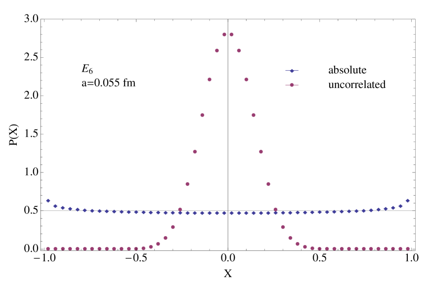
Figure 1: Absolute $X$–distribution in duality and reference $X$–distribution of statistically independent duality components for ensemble $E_{6}$.

5. Main Results. We have computed absolute $X$-distributions in duality for all ensembles listed in Table 1. The plot of Fig. 1 shows the result for ensemble $E_{6}$ which has the largest physical volume. Note that the associated kinematical background represented by the reference $X$–distribution of statistically independent components is also shown. As can be clearly seen, despite the completely “unpolarized–looking” kinematics, there is a slight dynamical tendency of the gauge field strength tensor to polarize itself. Indeed, the absolute $X$–distribution shows a small excess of probability near the extremal values of absolute polarization coordinate. This observation represents the central message of this work since, as we discuss below, the data suggests that such dynamical behavior persists both in the continuum and infinite volume limits.

Focusing on absolute $X$-distributions from now on, we show them more closely for all ensembles with fixed physical volume in Fig. 2. As can be directly inspected, these distributions are all mildly convex, implying small positive dynamical tendency for polarization in duality. Despite the fact that this tendency slowly decreases toward the continuum limit, the data strongly suggests that a finite positive continuum limit does exist. In Fig. 2 we also show a fit to quadratic polynomial in lattice spacing, which we take to facilitate this continuum extrapolation.

  

  

  

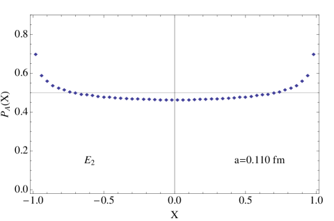
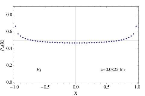
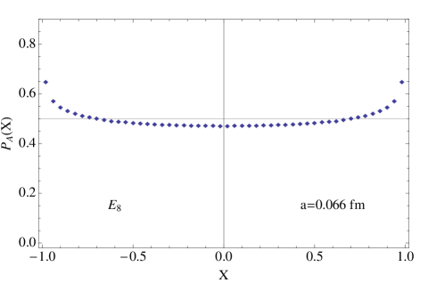
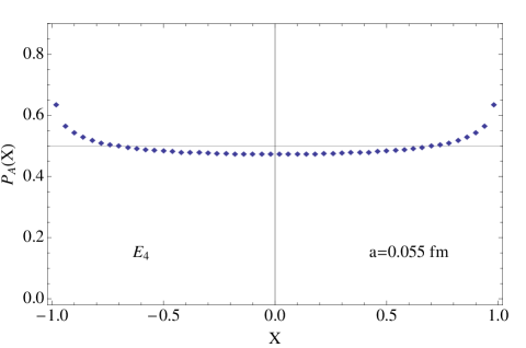
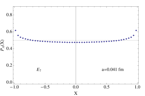
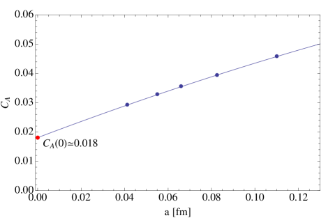
Figure 2: Absolute duality $X$–distributions for all ensembles at fixed physical volume $V=(1.32\,{\mbox{\rm fm}})^{4}$. Lattice spacing is decreasing in lexicographic order of plots. The last panel shows the corresponding lattice spacing dependence of the polarization correlation coefficient, together with the quadratic fit for extrapolation to the continuum limit. All data points in the above plots have errorbars too small to be clearly seen.

Although the physical volume in the above continuum extrapolation is rather small, the finite volume corrections for observables at hand turn out to be negligible. Indeed, in Fig. 3 we show the comparison of absolute $X$–distributions for ensembles $E_{4}$ and $E_{6}$ that have identical couplings ($a=0.055$ fm) but with $E_{6}$ representing a significantly larger physical volume. As can be seen in this close–up view, the two distributions are rather difficult to distinguish one from another.

The above results make strong case for the following proposition that we suggest for further investigation.

Proposition 1:  Absolute $X$–distributions for duality in SU(3) pure glue lattice gauge theory are convex. This property, and thus the associated positive tendency for (anti)self–duality, will persist in the continuum limit.

It needs to be emphasized that the observed polarization tendency, as objectively quantified by the associated correlation coefficient, is very small. In particular, $C_{A}\approx 0.018$ for continuum limit taken using Iwasaki lattice gauge action and overlap-based definition of the field–strength tensor.

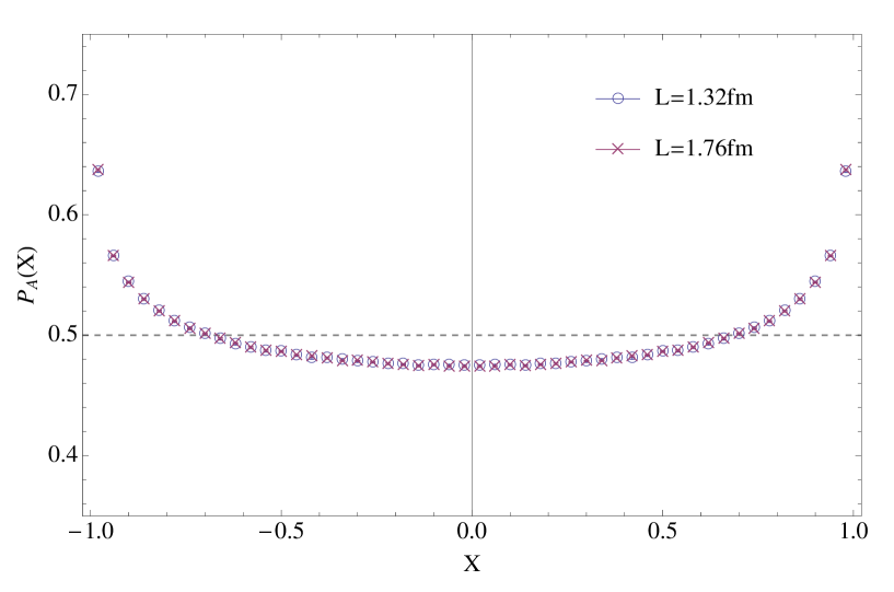
Figure 3: The comparison of absolute $X$–distributions at the same lattice spacing but different volumes ($E_{4}$ and $E_{6}$).

6. Effective Field Strength Tensor. It is revealing to compare dynamical polarization tendencies of fully fluctuating field strength to those of effective fields defined by equation (12). In Fig.4 (top right) we show the comparison of absolute $X$–distributions for $F$ and $F^{\Lambda}$, $\Lambda=1000$ MeV, in ensemble $E_{4}$. The construction of effective field strength in this case involved the inclusion of $47$ overlap near–zero modes on average. As one can see, while the dynamical polarization tendency has somewhat increased in the effective field, the two cases do not differ qualitatively at all. This happens despite the fact that the associated reference $X$–distributions, which are only kinematic, differ significantly (top left of Fig.4). In the bottom panel of Fig.4 we added to the continuum extrapolation plot of Fig.2 the correlation coefficients $C_{A}$ at $\Lambda=1000$ MeV for ensembles with available eigenmodes. This shows that the correlation coefficients in the effective field are of comparable magnitudes to those for full field strength, and more so in the continuum limit.

Effective fields at fermionic scale $\Lambda$ suppress short distance fluctuations regardless of whether they contribute dynamically or represent pure noise. The above comparison thus speaks to the fact that absolute polarization measure has little sensitivity to the presence of noise, as emphasized in the opening remarks, and to the fact that the dynamical self–duality effect is mainly due to low–energy fields.

  

  

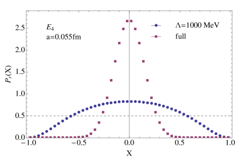
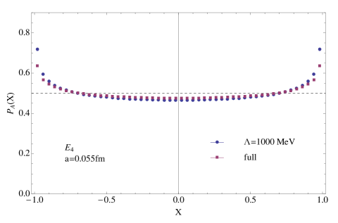
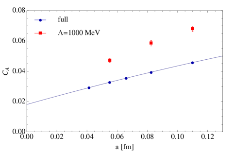
Figure 4: Comparison of dynamical polarization properties for field strength tensor $F$ and the effective field strength $F^{\Lambda}$, $\Lambda=1000$ MeV. See discussion in the text.

7. Discussion. In this work we constructed dynamical measures of self–duality in the gauge field. These measures are based on the notion of absolute $X$–distribution [14] which in turn represents a differential correlational characteristic of polarization. From the conceptual standpoint, this is an important step forward from initial approaches of Refs. [11, 13] that are only kinematical, and thus arbitrary. Indeed, not even a sign of dynamical tendency can be deduced from such results.

Using the above framework, we performed a detailed study of self–duality in pure–glue SU(3) gauge theory using lattice regularization. Our results indicate that this theory involves positive dynamical tendency for self–duality, meaning that QCD dynamics produces enhancement of self–duality relative to statistical independence in duality components. However, the observed effect is very weak. Indeed, the measured correlation coefficient is only ${C}_{A}\approx 0.018$ while, for example, it is straightforward to prescribe dynamics for measured marginal distributions of duality components, that would enhance this correlation at least 20–30 times. It is significant in this regard that the same is true for low–energy effective fields obtained via eigenmode expansion of the field–strength tensor, despite of the associated “noise reduction”. We are thus led to conclude that self–duality, and hence classicality, does not manifest itself as a significant feature of pure–glue QCD dynamics. This is consistent with previous arguments [4, 24, 8] as well as with lattice QCD studies [8, 9, 25, 10] indicating an intrinsically non–classical paradigm of QCD topological charge fluctuations.

Acknowledgments: Andrei Alexandru is supported in part by U.S. Department of Energy under grant DE-FG02-95ER-40907. Ivan Horváth acknowledges warm hospitality of the BNL Theory Group during which part of this work has been completed.

References

- [1] A.M. Polyakov, Phys. Lett. 59B, 82 (1975); Nucl. Phys. B121, 429 (1977); A.A. Belavin, A.M. Polyakov, A. Schwartz, Y. Tyupkin, Phys. Lett. 59B, 85 (1975).
- [2] G. ’t Hooft, Phys. Rev. Lett. 37, 8 (1976); Phys. Rev. D14, 3432 (1976).
- [3] C. Callan, R. Dashen, D.J. Gross, Phys. Lett. 63B, 334 (1976); R. Jackiw and C. Rebbi, Phys. Rev. Lett. 37, 172 (1976).
- [4] E. Witten, Nucl. Phys. B149, 285 (1979); Nucl. Phys. B256, 269 (1979).
- [5] C.G. Callan, R. Dashen, D.J. Gross, Phys. Rev. D17, 2717 (1978).
- [6] E.V. Shuryak, Nucl. Phys. B198, 83 (1982); D.I. Diakonov and V.Y. Petrov, Nucl. Phys. B245, 259 (1984); T. Schäfer, E. Shuryak, Rev. Mod. Phys. 70, 323 (1998).
- [7] D.I. Diakonov, V.Y. Petrov, Nucl. Phys. B272, 457 (1986).
- [8] I. Horváth, S.J. Dong, T. Draper, F.X. Lee, K.F. Liu, H.B. Thacker, J.B. Zhang, Phys. Rev. D67, 011501 (2003).
- [9] I. Horváth, S.J. Dong, T. Draper, F.X. Lee, K.F. Liu, N. Mathur, H.B. Thacker, J.B. Zhang, Phys. Rev. D68, 114505 (2003).
- [10] E.M. Ilgenfritz, K. Koller, Y. Koma, G. Schierholz, T. Streuer, V. Weinberg, Phys. Rev. D76, 034506 (2007).
- [11] I. Horváth, N. Isgur, J. McCune, H.B. Thacker, Phys. Rev. D65, 014502 (2002).
- [12] M. Creutz, Acta Physica Slovaca 61, No.1, 1 (2011). [arXiv:1103.3304]
- [13] C. Gattringer, Phys. Rev. Lett. 88, 221601 (2002).
- [14] A. Alexandru, T. Draper, I. Horváth, T. Streuer, Annals Phys. 326, 1941 (2011), arXiv:1009.4451.
- [15] T. Draper et al, Nucl. Phys. B (Proc. Suppl.) 140, 623 (2005), arXiv:hep-lat/0408006.
- [16] T. DeGrand, A. Hasenfratz, Phys. Rev. D65, 014503 (2002); T. Blum et al, Phys. Rev. D65, 014504 (2002); I. Hip et al., Phys. Rev. D65, 014506 (2002); R. Edwards, U. Heller, Phys. Rev. D65, 014505 (2002); C. Gattringer et al., Nucl. Phys. B618 (2001) 205; Nucl. Phys. B617 (2001) 101; I. Horváth et al., Phys. Rev. D66, 034501 (2002).
- [17] Y. Iwasaki, Nucl. Phys. B258 (1985) 141.
- [18] M. Okamoto et al. Phys. Rev. D60, 094510 (1999).
- [19] I. Horváth, hep-lat/0607031.
- [20] K.F. Liu, A. Alexandru, I. Horváth, Phys. Lett. B659 (2008) 773.
- [21] A. Alexandru, I. Horváth, K.F. Liu, Phys. Rev. D78, 085002 (2008).
- [22] H. Neuberger, Phys. Lett. B417 (1998) 141; Phys. Lett. B427 (1998) 353.
-
[23]
D.C. Sorensen, SIAM J. Matrix Anal. Appl 13 (1992) 357.
R.B. Lehoucq, D.C. Sorensen, SIAM J. Matrix Anal. Appl 17 (1996) 789. - [24] E. Witten, Phys. Rev. Lett. 81, 2862 (1998).
- [25] I. Horváth, A. Alexandru, J.B. Zhang, S.J. Dong, T. Draper, F.X. Lee, K.F. Liu, N. Mathur, H.B. Thacker, Phys. Lett. B612 (2005) 21.