On the temporal Wilson loop in the Hamiltonian approach in Coulomb gauge

Abstract

We investigate the temporal Wilson loop using the Hamiltonian approach to Yang-Mills theory. In simple cases such as the Abelian theory or the non-Abelian theory in $(1+1)$ dimensions, the known results can be reproduced using unitary transformations to take care of time evolution. We show how Coulomb gauge can be used for an alternative solution if the exact ground state wave functional is known. In the most interesting case of Yang-Mills theory in $(3+1)$ dimensions, the vacuum wave functional is not known, but recent variational approaches in Coulomb gauge give a decent approximation. We use this formulation to compute the temporal Wilson loop and find that the Wilson and Coulomb string tension agree within our approximation scheme. Possible improvements of these findings are briefly discussed.

I Introduction

In recent years there has been a renewed interest in studying Yang-Mills theory in Coulomb gauge, both in the continuum Zwanziger (2003) and on the lattice Langfeld and Moyaerts (2004); Quandt et al. (2007); Voigt et al. (2007, 2008); Burgio et al. (2009, 2010); Quandt et al. (2010). These developments are mainly based on the fact that the consequences of the Gribov-Zwanziger picture of confinement Gribov (1978); Zwanziger (1997) are particularly transparent in Coulomb gauge: Physical states in the Hamiltonian formulation have to obey Gauss’ law, without the need of additional restrictions such as a vanishing color charge based, in turn, on the assumption of a globally conserved BRST charge. Furthermore, since Gauss’ law can be resolved explicitly in Coulomb gauge, any renormalizable Ansatz for a vacuum wave functional is admissible in this gauge without having to explicitly construct the physical Hilbert space Burgio et al. (2000), which is a key fact to make variational approaches viable. (The equivalent Gupta-Bleuler type of constraints in covariant gauges have no such simple resolution.)

Consequently, much work was devoted to a variational solution of the Yang-Mills Schrödinger equation in Coulomb gauge Szczepaniak and Swanson (2002); Feuchter and Reinhardt (2004, 2004); Reinhardt and Feuchter (2005); Epple et al. (2007, 2008); Reinhardt and Schleifenbaum (2009); Schleifenbaum et al. (2006); Reinhardt and Epple (2007). Using Gaussian type of Ansätze for the vacuum wave functional, a set of Dyson-Schwinger equations for the gluon and ghost propagators was derived by minimizing the vacuum energy density. An infrared analysis Schleifenbaum et al. (2006) of these equations exhibits solutions in accord with the Gribov-Zwanziger confinement scenario. Imposing Zwanziger’s horizon condition one finds an infrared diverging gluon energy and a linear rising static quark (Coulomb) potential Schleifenbaum et al. (2006) and also a perimeter law for the ’t Hooft loop Reinhardt and Epple (2007). These infrared properties are reproduced by a full numerical solution of the Dyson-Schwinger equations over the entire momentum regime Epple et al. (2007), and are also supported by lattice calculations Quandt et al. (2007); Burgio et al. (2009). Moreover, since the inverse of the ghost dressing function can be identified with the dielectric function of the Yang-Mills vacuum Reinhardt (2008), the latter behaves in the infra-red, by the horizon condition, like a perfect color dia-electric medium, i.e. a dual superconductor. This suggests that the linearly rising Coulomb potential is a manifestation of confinement via the dual Meissner effect.

These nice physical conclusions are, however, a bit premature. Using variational arguments, one can show that the Coulomb potential is only an upper bound for the true potential between heavy quarks, which implies "no confinement without Coulomb confinement" Zwanziger (2003), but not the converse. To get a sufficient criterion for confinement, one has to study the true potential extracted from the temporal Wilson loop. In the non-Abelian continuum theory, the Wilson loop is difficult to calculate because of path ordering. In ref. Pak and Reinhardt (2009), the spatial Wilson loop was computed from a Dyson–Schwinger equation, which has previously been derived in ref. Erickson et al. (2000) in the context of supersymmetric Yang-Mills theory. Although a linearly rising potential was extracted from the obtained Wilson loop, it is not clear to which extend this approach also applies to non-supersymmetric Yang-Mills theory.

As was clarified in ref. Haagensen and Johnson (1997), it is by no means trivial to extract the static potential from the Wilson loop even in simple cases such as QED, due to the presence of singular self-energy terms. Another attempt to extract the static Coulomb potential of QED from the Wilson loop was undertaken in ref. Gaete (1999), where a partial wave expansion has been used. We have not been able to reproduce the result of ref. Gaete (1999) for the static potential in QED, and we reconsider the relevant partial wave expansion in appendix A. In the present paper, we will instead show that the proper and elegant way to extract the QED potential from the Wilson loop should be based on a separation of longitudinal and transversal degrees of freedom. In Coulomb gauge, this separation is accomplished automatically, which is the main reason why this particular gauge is so convenient for our purposes.

In the present paper, we will attempt to extract the static quark potential from the Wilson loop within the Hamiltonian approach, using gauge-invariant and Coulomb gauge techniques in exactly solvable cases, and approximate results from variational calculations for the most interesting case of non-Abelian Yang-Mills theory in $D=3+1$.

Our paper is organized as follows: In the next section, we demonstrate how a unitary transformation similar to the one that leads to the interaction picture in quantum mechanics gives rise to an induced electric field that allows to compute the Wilson potential exactly in special cases. To prepare for the non-Abelian theory in $(3+1)$ dimensions, we also show how Coulomb gauge can be incorporated in these exactly solvable models. In section 3, we first treat the case of an Abelian $U(1)$ theory reproducing the usual Coulomb potential from Maxwell’s theory. Section 4 treats Yang-Mills theory in $(1+1)$ dimensions on a cylindrical spacetime manifold. Finally, section five employs the known Gaussian wave functional from variational approaches to compute, with additional approximations, the Wilson string tension, which happens to agree with the Coulomb string tension within the given approximation scheme. We conclude with a brief summary and an outlook on further improvements of our calculation.

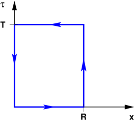
Figure 1: Temporal rectangular Wilson loop.

II The temporal Wilson loop in the Hamilton approach

Below, we investigate the temporal Wilson loop in the Hamiltonian approach to $SU(N)$ Yang-Mills theory. This formulation assumes the Weyl gauge, $A_{0}=0$, leaving a residual symmetry under spatial gauge rotations. Since the Wilson loop operator is gauge invariant, it is not necessary to further fix this residual symmetry in all cases. In fact, we will show that a gauge-invariant Hamiltonian treatment of the temporal Wilson loop is successful in simple cases, while more complex situations require gauge fixing as a technical tool to simplify the separation of physical degrees of freedom.

II.1 Physical interpretation

We consider a planar time-like Wilson loop as shown in figure 1. If the (Euclidean) time coordinate $\tau=x_{0}$ is unrestricted, the Weyl gauge $A_{0}=0$ can be adopted and the Wilson loop operator in the quark representation $r$ reads

$$W=\frac{1}{d_{r}}\,\mathrm{tr}_{r}\,\Big{[}U[\mathbf{A}](\mathbf{0},\mathbf{R}\,;\,\tau=T)\cdot U[\mathbf{A}](\mathbf{R},\mathbf{0}\,;\,\tau=0)\Big{]}=\mathrm{tr}\Big{[}U[\mathbf{A}](\mathbf{R},\mathbf{0}\,;\,T)^{\dagger}\cdot U[\mathbf{A}](\mathbf{R},\mathbf{0}\,;\,0)\Big{]}\hskip 2.84544pt,$$ (1)

where $tr_{r}$ is the trace in the $SU(N)$ representation $r$, $d_{r}\equiv\mathrm{tr}_{r}\,\mathbbm{1}$ is its dimension and $\mathrm{tr}\equiv d_{r}^{-1}\,\mathrm{tr}$ denotes the normalised trace. Furthermore, the parallel transporter along the path $\mathscr{C}$ running from $\mathbf{x}_{1}$ to $\mathbf{x}_{2}$ at the time $x_{0}=\tau$ is given by

$$U[\mathbf{A}]\left(\mathbf{x}_{2},\mathbf{x}_{1}\,;\,\tau\right)=\mathsf{P}\exp\left[-\int\limits_{\mathscr{C}\,:\,{\mbox{\boldmath$\scriptstyle{x}$\unboldmath}}_{1}\to{\mbox{\boldmath$\scriptstyle{x}$\unboldmath}}_{2}}d\mathbf{x}\,\mathbf{A}(\mathbf{x},\tau)\right]\,.$$ (2)

In this expression, we have absorbed the gauge coupling $g$ in the connection $\mathbf{A}$, which entails that the Yang-Mills Hamiltonian (in the absence of gauge fixing) takes the form

$$H = \frac{g^{2}}{2}\int dx\,\mbox{\boldmath$\Pi$\unboldmath}^{2}+\frac{1}{2g^{2}}\int dx\,\mathbf{B}^{2}\,,$$ (3)

$$\Pi^{a}_{k}(x) = -i\,\frac{\delta}{\delta A^{a}_{k}(x)}\,,\qquad\quad B^{a}_{k}(x)=\epsilon_{k\ell m}\,\partial_{\ell}\,A^{a}_{m}(x)+f^{abc}\,A_{\ell}^{b}(x)\,A_{m}^{c}(x)\,.$$ (4)

The time evolution of the gauge field in Euclidean space is then formally

$$\mathbf{A}(\mathbf{x},\tau)=e^{-H\tau}\,\mathbf{A}(\mathbf{x},0)\,e^{H\tau}\,.$$

and it is easy to see that the same semi-group law applies to the parallel transporter, so that the vev of the Wilson loop becomes

$$\langle\,W\,\rangle=\mathrm{tr}\,\langle\,0\,|\,U^{\dagger}(\mathbf{R})\,e^{-(H-E_{0})T}\,U(\mathbf{R})\,|\,0\,\rangle\hskip 2.84544pt=\mathrm{tr}\,\langle\,\mathbf{R}\,|\,e^{-T(H-E_{0})}\,|\,\mathbf{R}\,\rangle\,.$$ (5)

Here, $E_{0}$ is the energy of the YM vacuum $|\,0\,\rangle$ and the abbreviation $U(\mathbf{R})=U[\mathbf{A}](\mathbf{R},\mathbf{0};\tau=0)$ for the straight line transporter $\mathbf{0}\to\mathbf{R}$ made from gauge fields at time $\tau=0$ was introduced.

The next step is to insert a complete set of energy eigenstates in the matrix element eq. (5). To do this properly, we have to recall that the Hamiltonian eq. (3) is accompanied by a Hilbert space which decomposes into charge subspaces by virtue of Gauss’ law,

$$\hat{\Gamma}^{a}(\mathbf{z})\,\Psi_{i_{1},\ldots i_{n}}(\mathbf{A}\,;\,\mathbf{x}_{1},\ldots,\mathbf{x}_{n})=-\left\{\sum_{\ell=0}^{n}\sum_{\{k_{\ell}\}}\left[T^{a}_{(r_{\ell})}\right]_{i_{\ell}k_{\ell}}\,\delta(\mathbf{z}-\mathbf{x}_{\ell})\prod_{m\neq\ell}\delta_{i_{m}k_{m}}\right\}\cdot\,\Psi_{k_{1},\ldots,k_{n}}(\mathbf{A}\,;\,\mathbf{x}_{1},\ldots\mathbf{x}_{n})$$ (6)

where the sum is over the color spins of static quarks with color representation $T_{r}$ located at positions $\mathbf{x}_{1},\ldots,\mathbf{x}_{n}$. Since the Gauss law operator $\Gamma^{a}(\mathbf{x})\equiv\hat{\mathbf{D}}^{ab}(\mathbf{x})\mbox{\boldmath$\Pi$\unboldmath}^{b}(\mathbf{x})$ commutes with the (gauge-invariant) Hamiltonian, the charge subspaces are invariant under the YM dynamics and mutually orthogonal. By Schur’s lemma, the Hamilton operator eq. (3) is thus proportional to the color unit matrix when acting on any of the charge subspaces. Moreover, the Gauss law operator generates time-independent gauge transformations $U(\mathbf{x})$, i.e. the iteration of eq. (6) states (in the absence of a vacuum angle $\theta=0$) that a physical state from the $n$-quark sector transforms under gauge rotations as

$$\Psi_{i_{1},\ldots,i_{n}}(\mathbf{A}^{U}\,;\,\mathbf{x}_{1},\ldots,\mathbf{x}_{n})=\sum_{k_{1},\ldots,k_{n}}\mathscr{D}^{(r_{1})}_{i_{1}k_{1}}[U(\mathbf{x}_{1})]\cdots\mathscr{D}^{(r_{n})}_{i_{n}k_{n}}[U(\mathbf{x}_{n})]\,\Psi_{k_{1},\ldots,k_{n}}(\mathbf{A}\,;\,\mathbf{x}_{1},\ldots,\mathbf{x}_{n})\,,$$ (7)

where $\mathscr{D}^{(r)}[\Omega]$ denotes the color matrix $\Omega$ in representation $r$. For notational simplicity, we will henceforth assume that the Wilson loop is in the fundamental representation, so that all representation symbols $\mathscr{D}^{(r)}$ can be omitted.

It is now trivial to see that the Wilson state Heinzl et al. (2008, 2008) $|\mathbf{R}\rangle=U(\mathbf{R})\,|0\rangle$ from eq. (5) corresponds to the charge sector with a quark at position $\mathbf{R}$ and an antiquark in the origin. In fact, the identity

$$\Gamma^{a}(\mathbf{z})U(\mathbf{R})=-\delta(\mathbf{z}-\mathbf{R})\,iT^{a}\,U(\mathbf{R})+\delta(\mathbf{z}-\mathbf{0})\,U(\mathbf{R})\,iT^{a}\,,$$ (8)

implies the matrix relation

$$\Gamma^{a}(\mathbf{z})\,|\,\mathbf{R}\,\rangle_{ij}=-\Big{\{}\delta(\mathbf{z}-\mathbf{R})\,(iT^{a})_{ik}\,\delta_{j\ell}-\delta(\mathbf{z})\,\delta_{ik}\,(iT^{a})_{\ell j}\Big{\}}\,|\,\mathbf{R}\,\rangle_{k\ell}\,,$$ (9)

which corresponds to eq. (6). For finite gauge transformations $\Omega$ acting on the Wilson state, the equivalent of eq. (7) is

$$|\,\mathbf{R}\,\rangle_{ij}\to\Omega(\mathbf{R})_{ik}\cdot|\,\mathbf{R}\,\rangle_{k\ell}\,\cdot\Omega(0)^{-1}_{\ell j}\,.$$

Finally, for quark and antiquark in the same color representation, it is often convenient to parallel transport the charges to the same local color frame so that the charge density matrix acts on a single spin index only. In the present case, this can be achieved by the identity

$$\big{[}U\cdot(iT^{a})\big{]}_{i\ell}=\big{[}U\,iT^{a}\,U^{\dagger}\big{]}_{ik}\cdot U_{k\ell}$$ (10)

so that eq. (8) takes the simpler form

$$\Gamma^{a}(\mathbf{z})\,U_{i\ell}(\mathbf{R})=\Big{\{}\delta(\mathbf{z})\,[U(\mathbf{R})\,iT^{a}\,U(\mathbf{R})^{\dagger}]_{ik}-\delta(\mathbf{z}-\mathbf{R})\,iT^{a}_{ik}\Big{\}}\,U_{k\ell}(\mathbf{R})\equiv-{\rho}^{a}_{ik}(\mathbf{z})\cdot U_{k\ell}(\mathbf{R})\,,$$ (11)

where the second spin index ($\ell$) is not affected. As a consequence of the parallel transport, the two charges at the endpoints of the Wilson line do not exactly compensate

$$Q^{a}=\int d\mathbf{z}\,\rho^{a}(\mathbf{z})=i\,\big{[}\,U(\mathbf{R})\,T^{a}\,U(\mathbf{R})^{\dagger}-T^{a}\,\big{]}\neq 0$$ (12)

unless the color group is Abelian. (In any case, however, $\mathrm{tr}\,Q^{a}=0$.)

Returning to eq. (5), we insert a complete set of energy eigenstates from all charge sectors, but only the states from the proper quark-antiquark sector will give a non-vanishing contribution,

$$\langle W\rangle=\mathrm{tr}\,\sum_{n}\langle\,0\,|\,U^{\dagger}(\mathbf{R})\,|\,n\,\rangle_{q\bar{q}}\cdot e^{-(H-E_{0})T}\cdot{}_{q\bar{q}}\langle\,n\,|\,U(\mathbf{R})\,|\,0\,\rangle=\sum_{n}\,e^{-T(E_{n}^{(q\bar{q})}-E_{0})}\,\|\langle\mathbf{R}\,|\,n\,\rangle_{q\bar{q}}\|^{2}\,,$$ (13)

where $\|\Omega\|^{2}\equiv\mathrm{tr}(\Omega^{\dagger}\Omega)$. In the limit of large Euclidean time extensions, we project out the static quark potential

$$-\lim_{T\to\infty}\,T^{-1}\,\ln\,\langle W\rangle=E_{0}^{(q\bar{q})}-E_{0}\equiv V(R)\,,$$

provided that the Wilson line has non-vanishing overlap with the true vacuum in the proper quark-antiquark sector. (We will come back to this issue in section IV below.)

II.2 Induced electric field

To proceed, we use the spatial parallel transporter $U(\mathbf{R})$ to induce a transformation similar to the one that leads to the interaction picture in quantum mechanics. For instance, the new Hamilton operator becomes

$$\widetilde{H}=U^{\dagger}(\mathbf{R})\,H\,U(\mathbf{R})\equiv\widetilde{H}(\mathbf{R})\,.$$ (14)

All transformed quantities will be $\mathbf{R}$-dependent and denoted, generally, by a tilde; they will also be color matrices in the representation chosen for the Wilson loop, although we will sometimes omit color indices for simplicity. For the transformed momentum operator, we obtain

$$\widetilde{\Pi}^{a}_{i}(\mathbf{x})=U^{\dagger}(\mathbf{R})\,\Pi^{a}_{i}(\mathbf{x})\,U(\mathbf{R})=\Pi^{a}_{i}(\mathbf{x})+\epsilon^{a}_{i}(\mathbf{x})\,,$$ (15)

where a new color electric flux field

$$\mbox{\boldmath$\epsilon$\unboldmath}^{a}(\mathbf{x})\equiv\int\limits_{\mathscr{C}\,:\,\mathbf{0}\to\mathbf{R}}d\mathbf{y}\,\delta(\mathbf{x}-\mathbf{y})\,iU(\mathbf{y})^{\dagger}\,T^{a}\,U(\mathbf{y})=\int\limits_{\mathscr{C}\,:\,\mathbf{0}\to\mathbf{R}}d\mathbf{y}\,\delta(\mathbf{x}-\mathbf{y})\,i\widetilde{T}^{a}(\mathbf{y})$$ (16)

with $\widetilde{T}^{a}(\mathbf{y})\equiv U(\mathbf{y})^{\dagger}\,T^{a}\,U(\mathbf{y})$ has emerged. The unitary transformation (15) removes the parallel transporters from the Wilson state so that the Wilson loop becomes the expectation value of the transformed time evolution operator in the Yang-Mills (zero charge) vacuum,

$$\langle\,W\,\rangle=\mathrm{tr}\,\langle\,0\,|\,e^{-T(\widetilde{H}-E_{0})}\,|\,0\,\rangle\,.$$ (17)

The effect of the Wilson lines is now shuffled into the kinetic term of the new Hamiltonian,

$$\widetilde{H}=\frac{g^{2}}{2}\int d^{3}x\,\Big{[}\mbox{\boldmath$\Pi$\unboldmath}^{a}(\mathbf{x})\,\mathbbm{1}+\mbox{\boldmath$\epsilon$\unboldmath}^{a}(\mathbf{x})\Big{]}^{2}+\frac{1}{2g^{2}}\int d^{3}x\,\mathbf{B}(\mathbf{x})^{2}\,\mathbbm{1}\,.\hskip 2.84544pt$$ (18)

Note that $\mbox{\boldmath$\epsilon$\unboldmath}^{a}(\mathbf{x})$ depends on the gauge field, so that $[\Pi^{a}(\mathbf{x}),\epsilon^{b}(\mathbf{x})]\neq 0$ which complicates the treatment of the new Hamiltonian considerably. The induced electric field satisfies Gauss’ law for the external charge density induced by the Wilson line,

$$[\,\hat{\mathbf{D}}^{ab}(\mathbf{x})\,,\,\mbox{\boldmath$\epsilon$\unboldmath}^{b}(\mathbf{x})\,]=U(\mathbf{R})^{\dagger}\,\rho^{a}(\mathbf{x})\,U(\mathbf{R})=iT^{a}\,\delta(\mathbf{x})-i\widetilde{T}^{a}(\mathbf{R})\,\delta(\mathbf{x}-\mathbf{R})\equiv\widetilde{\rho}^{a}(\mathbf{x})\,.$$ (19)

This charge density $\widetilde{\rho}(\mathbf{x})$ is again a color matrix similar to eq. (11).

Before proceeding, let us briefly discuss the piece in the transformed Hamiltonian (18) which is quadratic in the induced electric field,

$$V_{\rm ind}[\mathscr{C}]=\frac{g^{2}}{2}\int d^{3}x\,\big{[}\mbox{\boldmath$\epsilon$\unboldmath}^{a}(\mathbf{x})\big{]}^{2}\,.$$ (20)

After a simple calculation using the definition of the quadratic Casimir operator $\widetilde{T}^{a}\,\widetilde{T}^{a}=T^{a}\,T^{a}=C_{2}\,\mathbbm{1}$, we find

$$V_{\rm ind}[\mathscr{C}]=\frac{g^{2}}{2}\,C_{2}\int\limits_{\mathscr{C}\,:\,\mathbf{0}\to\mathbf{R}}d\mathbf{x}\,\int\limits_{\mathscr{C}\,:\,\mathbf{0}\to\mathbf{R}}d\mathbf{y}\,\delta^{3}(\mathbf{x}-\mathbf{y})\,\mathbbm{1}\hskip 2.84544pt.$$ (21)

This term is independent of the gauge field and thus also of the vacuum wave functional used, but it does depend on the shape of the contour $\mathscr{C}\,:\,\mathbf{0}\to\mathbf{R}$ in the spatial part of the Wilson loop. Choosing $\mathscr{C}$ to be a straight line connecting $\mathbf{0}$ and $\mathbf{R}$, we have

$$V_{\rm ind}[\mathscr{C}]=\frac{g^{2}}{2}\,C_{2}\,\delta^{2}_{\perp}(0)\cdot|\mathbf{R}|\,\mathbbm{1}\hskip 2.84544pt\,.$$ (22)

The color unit matrix disappears when the trace of the Wilson loop is taken. While eq. (22) is formally a linearly rising potential, the corresponding string tension

$$\frac{g^{2}}{2}\,C_{2}\,\delta^{2}_{\perp}(0)=\frac{\Lambda^{2}}{8\pi}\,g^{2}\,C_{2}$$ (23)

is UV-divergent (cutoff $\Lambda$) and of purely kinematic origin. Except for the Casimir operator $C_{2}\to 1$, the same contribution is also found in the case of QED which does not confine; so it must be spurious. In fact, the singular energy is due to the infinitely thin Wilson lines whose point-like cross section gives rise to the factor $\delta^{2}_{\perp}(0)$ in eq. (23). If the lines are smeared out to an effective tube with cross section $\sim\Lambda^{-2}$, the self-energy is regularized, $\delta^{2}_{\perp}(0)\sim\Lambda^{2}$, but it will still obscure the physical potential unless it is properly isolated and removed.

To see the origin of the problem in more detail, consider the Abelian case where Gauss’ law for the induced electric field, $\nabla\mbox{\boldmath$\epsilon$\unboldmath}=\rho$, indicates that only the longitudinal part of $\epsilon$ is sensitive to external charges. As a consequence, the static potential (20) decomposes into two parts,

$$V_{\rm ind}[\mathscr{C}]=\frac{g^{2}}{2}\,\int d^{3}x\,\big{[}\mbox{\boldmath$\epsilon$\unboldmath}_{\perp}(\mathbf{x})\big{]}^{2}+\frac{g^{2}}{2}\,\int d^{3}x\,\big{[}\mbox{\boldmath$\epsilon$\unboldmath}_{\|}(\mathbf{x})\big{]}^{2}\equiv V_{\perp}[\mathscr{C}]+V_{\|}[\mathscr{C}]\,.$$

The first piece $V_{\perp}$ is built from $\mbox{\boldmath$\epsilon$\unboldmath}_{\perp}$ alone and thus insensitive to external charges; it represents a vacuum property that renormalizes the Wilson loop but does not affect the physical potential between static quarks. The latter is given exclusively by the second piece $V_{\|}$ which will be shown below to describe the well-known Coulomb interaction. The separation of transversal and longitudinal degrees of freedom is thus essential to disentangle the physical potential from renormalization effects. In ref. Gaete (1999), a different approach to remove the self-energies of the Wilson line and to isolate the proper quark potential was proposed, which is based on partial wave expansion. Appendix A compares this method to our reasoning based on Gauss’ law.

II.3 Coulomb gauge

Gauge invariant calculations of the Wilson loop are only possible in special cases where the exact ground state is known analytically. In realistic cases, the vacuum wave functional is unknown and one has to resort to approximate calculations which usually require some sort of gauge fixing. For the Hamiltonian approach, Coulomb gauge is a natural choice which simplifies the separation of dynamical from gauge degrees of freedom. In QED, for instance, the Coulomb gauge fixed field represents the physical (gauge invariant) degrees of freedom.

Not surprisingly, the variational approach to YM theory in Coulomb gauge has recently become an excellent tool to obtain approximate ground state wave functionals which are suitable for practical computations. We will use this approach for YM-theory in $D=3+1$ in section V.

In view of our previous analysis, we can choose to fix the Coulomb gauge either before or after the unitary transformation (14) that led from expression (5) to eq. (17). That is, starting from the invariant Hamiltonian $H$ in eq. (3), we can either

1. gauge fix $H$ directly and compute $\langle W\rangle$ from eq. (5): $\quad\langle W\rangle=\mathrm{tr}\,\left\langle\,\mathbf{R}\,\left|\,e^{-T(H-E_{0})}\,\right|\,\mathbf{R}\,\right\rangle$

   The gauge fixed Coulomb Hamiltonian can be obtained either by canonical or by path integral techniques. The well-known result is the expression Christ and Lee (1980)

   $$H = \frac{g^{2}}{2}\,\int d^{3}x\,\mathscr{J}^{-1}\,\mbox{\boldmath$\Pi$\unboldmath}^{\perp}_{a}(\mathbf{x})\,\mathscr{J}\,\mbox{\boldmath$\Pi$\unboldmath}^{\perp}_{a}(\mathbf{x})+\frac{1}{2g^{2}}\,\int d^{3}x\,\big{[}\,\mathbf{B}^{a}(\mathbf{x})\,\big{]}^{2}+H_{C}$$ (24)

   $$H_{C} = \frac{g^{2}}{2}\,\int d^{3}(x,y)\,\mathscr{J}^{-1}\,\big{[}\rho^{a}(\mathbf{x})+\rho^{a}_{\rm dyn}(\mathbf{x})\big{]}\,\mathscr{J}\cdot F^{ab}(\mathbf{x},\mathbf{y})\,\big{[}\rho^{b}(\mathbf{y})+\rho_{\rm dyn}^{b}(\mathbf{y})\big{]}\,,$$ (25)

   where $\mathscr{J}[A]=\det(-\hat{\mathbf{D}}\nabla)$ is the Faddeev–Popov determinant and the Coulomb kernel $F$ reads

   $$F=(-\hat{\mathbf{D}}\nabla)^{-1}(-\Delta)\,(-\hat{\mathbf{D}}\nabla)^{-1}\,.$$

   The resolution of Gauss’ law must take into account that the state $|\,\mathbf{R}\,\rangle$ in eq. (5) is charged, i.e. besides the dynamical charge of the gluons, $\rho_{\rm dyn}^{a}(\mathbf{x})\equiv-\hat{\mathbf{A}}^{ab}_{\perp}(\mathbf{x})\,\mbox{\boldmath$\Pi$\unboldmath}^{b}_{\perp}(\mathbf{x})$ (with $\hat{A}_{\perp}^{ab}\equiv f^{acb}\,A_{\perp}^{c}$), we also have to include the external charge $\rho^{a}$ induced by the Wilson line. For instance, from Gauss’ law in the form eq. (11)

   $$\big{(}\hat{\mathbf{D}}^{ab}\,\mbox{\boldmath$\Pi$\unboldmath}^{b}\big{)}\,\Psi_{ij}=-\rho^{a}_{ik}\,\Psi_{kj}\qquad\Longrightarrow\qquad\nabla\mbox{\boldmath$\Pi$\unboldmath}^{a}\,\Psi_{ij}=-\big{[}\rho^{a}+\rho_{\rm dyn}^{a}\,\mathbbm{1}\big{]}_{ik}\,\Psi_{kj}$$

   the usual resolution entails that the charges in eq. (25) are really matrices $[\rho^{a}+\rho^{a}_{\rm dyn}\,\mathbbm{1}]$, and so is the Coulomb kernel $H_{C}$. The Wilson state $|\,\mathbf{R}\,\rangle$, after gauge fixing, depends on $\mathbf{A}^{\perp}$ only and is thus no longer from the $q\bar{q}$-sector; it will, in fact, have overlap with the zero-charge sector.

2. compute $\widetilde{H}=U(\mathbf{R})\,H\,U(\mathbf{R})^{\dagger}$ and gauge fix expression eq. (17): $\langle W\rangle=\langle\,0\,|\,\mathrm{tr}\,e^{-T(\widetilde{H}-E_{0})}\,|\,0\,\rangle$

   Since the Wilson lines have been taken care of by the unitary transformation $H\to\widetilde{H}$ in eq. (14), no further external charges have to be included, and Gauss’ law takes the form $\hat{\mathbf{D}}\hat{\mbox{\boldmath$\Pi$\unboldmath}}\,|\,0\,\rangle=0$. All calculations can thus be done in the zero-charge sector. From eq. (18), we could now follow the standard route and apply the Faddeev–Popov procedure to the vev

   $$\langle\,0\,|\,\widetilde{H}\,|\,0\,\rangle=\int\mathscr{D}\mathbf{A}\,\big{[}(\mbox{\boldmath$\Pi$\unboldmath}+\mbox{\boldmath$\epsilon$\unboldmath})\,\Psi_{0}\big{]}^{\ast}\,\big{[}(\mathbf{\Pi}+\mathbf{\epsilon})\,\Psi_{0}\big{]}+\cdots\,\qquad\quad\Psi_{0}[\mathbf{A}]\equiv\langle\,\mathbf{A}\,|\,0\,\rangle\,.$$

   Using Gauss’ law to solve for $\mathbf{\Pi}^{\|}\,\Psi_{0}$ eliminates all longitudinal d.o.f. and yields the vev $\langle\,0\,|\,\widetilde{H}^{\perp}\,|\,0\,\rangle$ in terms of transversal fields only. However, this is usually not sufficient to find the required vev of the gauge fixed evolution operator $\langle\,0\,|e^{-T\widetilde{H}^{\perp}}\,|\,0\,\rangle$, except for special cases such as QED.

Thus for the non-Abelian case, we prefer to follow the first method based on the standard Coulomb gauge Hamiltonian, while Abelian systems can be treated with both approaches.

III Quantum electrodynamics

III.1 Gauge invariant treatment

In the Abelian case $G=U(1)$, the Maxwell gauge potentials do not carry a color index, and the hermitian generator of the non-Abelian gauge group, $(iT^{a})$, has to be replaced by $1$, so that also $C_{2}=1$. The formula for the induced electric field in the representation eq. (18) simplifies to

$$\mbox{\boldmath$\epsilon$\unboldmath}(\mathbf{x})=\int\limits_{\mathscr{C}}d\mathbf{y}\,\delta^{(3)}(\mathbf{x}-\mathbf{y})\,.$$ (26)

In particular, $\mbox{\boldmath$\epsilon$\unboldmath}(\mathbf{x})$ is field-independent and the parallel transporter $\mathbf{0}\to\mathbf{R}$ becomes

$$U(\mathbf{R})=\exp\left[i\int d^{3}x\,\mbox{\boldmath$\epsilon$\unboldmath}(\mathbf{x})\cdot\mathbf{A}(\mathbf{x})\right].$$

To isolate the physical degrees of freedom, we split all vector fields in longitudinal and transversal parts. Without gauge fixing, the ground state $\Psi_{0}[\mathbf{A}]=\langle\,\mathbf{A}\,|\,0\,\rangle$ is eigenstate of the gauge invariant Hamiltonian, and thus gauge invariant itself; as a consequence, it can only depend on the physical (i.e. transversal) field $\mathbf{A}^{\perp}$ , so that $\mbox{\boldmath$\Pi$\unboldmath}^{\|}\,|\,0\,\rangle=0$. From eq. (17) and (18), this entails

$$\langle\,W\,\rangle = \left\langle\,0\,\left|\,e^{-T\left(\widetilde{H}_{\rm QED}^{\perp}-E_{0}\right)}\,\right|\,0\,\right\rangle$$

$$\widetilde{H}_{\rm QED}^{\perp} = \frac{1}{2}\int d^{3}x\left[g^{2}\,\big{[}\mathbf{\Pi}^{\perp}(x)+\mbox{\boldmath$\epsilon$\unboldmath}^{\perp}(x)\big{]}^{2}+\frac{1}{g^{2}}\,\mathbf{B}^{2}(x)+g^{2}\,\big{[}\mbox{\boldmath$\epsilon$\unboldmath}^{\|}(x)\big{]}^{2}\right]\,.\hskip 2.84544pt$$ (27)

Since $\epsilon$ is independent of the gauge field, the last term in $\widetilde{H}_{\rm QED}^{\perp}$ commutes with the remainder and can be pulled out of the vev,

$$\langle\,W\,\rangle = e^{-TV^{\|}}\cdot\left\langle\,0\,\left|\,e^{-T\left(\widetilde{H}_{\rm QED}^{\prime}-E_{0}\right)}\,\right|\,0\,\right\rangle$$

$$V^{\|} = \frac{g^{2}}{2}\,\int d^{3}\mathbf{x}\,\big{[}\mbox{\boldmath$\epsilon$\unboldmath}^{\|}(\mathbf{x})\big{]}^{2}\,,$$ (28)

where $V_{\|}$ is the part of the induced static potential that is sensitive to external charges, cf. our previous discussion. The remaining Hamiltonian

$$\widetilde{H}_{\rm QED}^{\prime}=\frac{1}{2}\int d^{3}x\left[g^{2}\,\big{[}\mathbf{\Pi}^{\perp}(\mathbf{x})+\mbox{\boldmath$\epsilon$\unboldmath}^{\perp}(\mathbf{x})\big{]}^{2}+\frac{1}{g^{2}}\,\big{[}\nabla\times\mathbf{A}^{\perp}(\mathbf{x})\big{]}^{2}\right]$$

depends on the physical degrees of freedom $\mathbf{A}^{\perp}$ only. It is most easily treated by reversing the transformation eq. (15), but this time with the parallel transporter made of physical gauge fields $\mathbf{A}^{\perp}$ only,

$$U^{\perp}(\mathbf{R})\equiv\exp\left[i\int_{\mathscr{C}\,:\,\mathbf{0}\to\mathbf{R}}d\mathbf{x}\,\mathbf{A}^{\perp}(\mathbf{x})\right]=\exp\left[i\int d^{3}\mathbf{x}\,\mbox{\boldmath$\epsilon$\unboldmath}^{\perp}(\mathbf{x})\cdot\mathbf{A}^{\perp}(\mathbf{x})\right]\,.$$ (29)

As a result, the induced transversal electric field $\mbox{\boldmath$\epsilon$\unboldmath}^{\perp}$ is removed from the Hamiltonian and re-shuffled into the state $|\,\mathbf{R}^{\perp}\,\rangle=U^{\perp}(\mathbf{R})\,|\,0\,\rangle$. Although this new state $|\,\mathbf{R}^{\perp}\,\rangle$ resembles the Wilson state, it depends on $\mathbf{A}^{\perp}$ only and is thus gauge invariant, i.e. $|\,\mathbf{R}^{\perp}\,\rangle$ lies in the zero-charge sector. Inserting a complete set of zero-charge (gauge invariant) eigenstates of the standard QED Hamiltonian,

$$H_{\rm QED}=\frac{1}{2}\int d^{3}x\left[g^{2}\,\big{[}\mathbf{\Pi}^{\perp}(\mathbf{x})\big{]}^{2}+\frac{1}{g^{2}}\,\big{[}\nabla\times\mathbf{A}^{\perp}(\mathbf{x})\big{]}^{2}\right]$$ (30)

with $\mbox{\boldmath$\Pi$\unboldmath}^{\perp}=\delta/i\delta\mathbf{A}^{\perp}$ we find

$$\langle\,W\,\rangle=e^{-TV_{\|}}\,\sum\limits_{n}e^{-\left(E_{n}-E_{0}\right)T}\,\left|\,\left\langle\,n\,\left|\,U^{\perp}(\mathbf{R})\,\right|\,0\,\right\rangle\,\right|^{2}\hskip 2.84544pt\,.$$ (31)

It is clear that only the first term ($n=0)$ in the sum survives in the limit $T\to\infty$, provided that the matrix element $\langle\,0\,|\,U^{\perp}(\mathbf{R})\,|\,0\,\rangle=\langle\,0\,|\,\mathbf{R}^{\perp}\,\rangle$ is non-vanishing. In the present case, this matrix element can be computed explicitly, since the vacuum wave functional is Gaussian,

$$\Big{\langle}\,\mathbf{A}^{\perp}(\mathbf{x})\,\Big{|}\,0\,\Big{\rangle}=\mathscr{N}\,\exp\left[-\frac{1}{g^{2}}\,\int d^{3}(x,y)\,\mathbf{A}^{\perp}(\mathbf{x})\,\omega(\mathbf{x},\mathbf{y})\,\mathbf{A}^{\perp}(\mathbf{y})\right]\,.$$

A simple Gaussian integral gives

$$\langle\,0\,|\,U^{\perp}(\mathbf{R})\,|\,0\,\rangle = \left\langle\,0\,\left|\,\exp\left[i\int d^{3}x\,\mathbf{A}^{\perp}(\mathbf{x})\cdot\mbox{\boldmath$\epsilon$\unboldmath}^{\perp}(\mathbf{x})\right]\,\right|\,0\,\right\rangle=$$

$$=\,\,\,\exp\left[-\frac{g^{2}}{4}\,\int d^{3}(x,y)\,\mbox{\boldmath$\epsilon$\unboldmath}^{\perp}(\mathbf{x})\,\omega^{-1}(\mathbf{x},\mathbf{y})\,\mbox{\boldmath$\epsilon$\unboldmath}^{\perp}(\mathbf{y})\right]=\exp\left[-\frac{g^{2}}{4}\,\int_{\mathbf{0}}^{\mathbf{R}}dx_{i}\int_{\mathbf{0}}^{\mathbf{R}}dy_{j}\,t_{ij}(\mathbf{x})\,\omega^{-1}(\mathbf{x},\mathbf{y})\right]\,,$$

where $t_{ij}$ is the usual transversal projector. This expression can be further evaluated if we choose the path $\mathbf{0}\to\mathbf{R}$ to be a straight line and employ the QED dispersion relation $\omega(\mathbf{k})=|\mathbf{k}|$ to invert the kernel $\omega(\mathbf{x},\mathbf{y})$ in momentum space. Introducing spherical coordinates in momentum space, the parameter integrals for the Wilson lines can be done first, while the subsequent angle integral can be expressed through the integral sinus, $\mathrm{Si}(x)$. For the remaining integral over $k=|\mathbf{k}|$, we use a sharp UV cutoff (i.e. a $O(3)$ invariant cutoff in 3-space), to find

$$\langle\,0\,|\,\mathbf{R}^{\perp}\,\rangle = \exp\left[-\frac{g^{2}}{8\pi^{2}}\left(4\gamma+2\cos(\Lambda R)-4\ln(\Lambda R)+4\,\mathrm{Ci}(\Lambda R)-2\,\frac{\sin(\Lambda R)}{\Lambda R}+2\,\Lambda R\,\mathrm{Si}(\Lambda R)\right)\,\right]$$ (32)

$$= \exp\left[-\frac{g^{2}}{8\pi^{2}}\left(\pi\Lambda R-4\ln(\Lambda R)-4\gamma+\mathscr{O}(\Lambda^{-3})\right)\,\right]\,.$$

In the limit $T\to\infty$, the bare Wilson loop thus becomes

$$\langle\,W\,\rangle=Z_{W}(\Lambda R)\cdot\exp\left[-T\,V_{\|}(R)\right]$$ (33)

where

$$Z_{W}(x)=\exp\left[-\frac{g^{2}}{4\pi^{2}}\,\left(\pi x-4\ln x-4\gamma\right)\right]\,.$$

Formally, $Z_{W}$ vanishes in the limit $\Lambda\to\infty$, which indicates that the state $|\,\mathbf{R}^{\perp}\,\rangle$ with support on an infinitely thin line has poor overlap with the true QED ground state. On the other hand, $Z_{W}$ is independent of $T$ and therefore does not contribute to the potential. The correct interpretation is given by the operator product expansion (OPE) Collins (1984): Since the Wilson loop $W$ is a composite operator involving products of arbitrarily many gauge fields, we expect short-distance OPE divergences associated with the operator $W$, in addition to those counter terms which are necessary to render elementary Green functions finite. Eq. (33) shows that this is indeed the case, with one overall multiplication of the operator $W\to W_{R}\equiv Z_{W}^{-1}\cdot W$ rendering all matrix elements finite. This renormalization property of Wilson loops is an exact result that has been known for a long time both in the Abelian and non-Abelian case Gervais and Neveu (1980); Polyakov (1980). From the renormalized value

$$\langle\,W_{R}\,\rangle=\exp\left[-T\,V^{\|}(R)\right]\,,\qquad\quad T\to\infty$$

we conclude that, in the Abelian case, the Wilson potential agrees with $V_{\|}$. A simple explicit calculation gives first the induced electric field

$$\mbox{\boldmath$\epsilon$\unboldmath}^{\|}(\mathbf{x}) = -\nabla_{x}\,(-\Delta_{x}^{-1})\,\nabla_{x}\,\mbox{\boldmath$\epsilon$\unboldmath}(\mathbf{x})=\nabla_{x}\,(-\Delta_{x}^{-1})\,\int_{\mathbf{0}}^{\mathbf{R}}dy\,\nabla_{y}\,\delta(\mathbf{x}-\mathbf{y})$$ (34)

$$\qquad\qquad=\,\,\,-\nabla_{x}\,(-\Delta_{x}^{-1})\,\left[-\delta(\mathbf{x}-\mathbf{R})+\delta(\mathbf{x})\right]\equiv-\nabla_{x}\,(-\Delta_{x}^{-1})\,\rho(\mathbf{x})$$

and thus Gauss’ law $\nabla\mbox{\boldmath$\epsilon$\unboldmath}^{\|}=\rho$. The Wilson potential becomes, after integration by parts and using the Green function $G(\mathbf{x},\mathbf{y})=\langle\,\mathbf{x}\,|\,(-\Delta)^{-1}\,|\,\mathbf{y}\,\rangle=(4\pi|\mathbf{x}-\mathbf{y}|)^{-1}$

$$V^{\|}(R) = \frac{g^{2}}{2}\,\int d^{3}\mathbf{x}\,\Big{[}\mbox{\boldmath$\epsilon$\unboldmath}^{\|}(\mathbf{x})\Big{]}^{2}=\frac{g^{2}}{2}\int d^{3}(\mathbf{x},\mathbf{y},\mathbf{z})\Big{[}-\nabla_{x}\,G(\mathbf{x},\mathbf{y})\,\rho(\mathbf{y})\Big{]}\cdot\Big{[}-\nabla_{x}\,G(\mathbf{x},\mathbf{z})\,\rho(\mathbf{z})\Big{]}=$$ (35)

$$= \frac{g^{2}}{2}\int d^{3}(\mathbf{x},\mathbf{y})\,\rho(\mathbf{x})\,G(\mathbf{x},\mathbf{y})\,\rho(\mathbf{y})=\frac{g^{2}}{2}\,\int d^{3}(\mathbf{x},\mathbf{y})\,\frac{\rho(\mathbf{x})\,\rho(\mathbf{y})}{4\pi\,|\mathbf{x}-\mathbf{y}|}=$$

$$= \frac{g^{2}}{4\pi|\mathbf{R}|}-\frac{g^{2}}{4\pi\,|\mathbf{0}|}\,.$$

This is just the familiar Coulomb law including the self-energy of the two charges.

III.2 Coulomb gauge

In the Abelian case, we can apply both methods described in section II.3 to evaluate the Wilson loop in Coulomb gauge:

1. In the Abelian case, the gauge fixed Hamiltonian eq. (24) simplifies considerably. From $\mathscr{J}=\mbox{const}$, $F=(-\Delta)^{-1}$ and $\rho_{\rm dyn}=0$, we have

   $$H=\frac{1}{2}\int d^{3}x\left[g^{2}\,\mathbf{\Pi}^{\perp}(\mathbf{x})^{2}+\frac{1}{g^{2}}\,\mathbf{B}(\mathbf{x})^{2}\right]+\frac{g^{2}}{2}\int d^{3}(x,y)\,\rho(\mathbf{x})(-\Delta)^{-1}(\mathbf{x},\mathbf{y})\,\rho(\mathbf{y})\equiv H_{\rm QED}+H_{C}\,.$$

   The second piece $H_{C}$ is a field-independent $c$-number, so that $e^{-TH}=e^{-T\,H_{\rm QED}}\cdot e^{-T\,H_{C}}$. Taking into account that $|\,\mathbf{R}\,\rangle=U[\mathbf{A}^{\perp}]\,|\,0\,\rangle$ and inserting a complete set of eigenstates of $H_{\rm QED}$, we arrive directly at eq. (31), from which we can follow all the steps to the final expression eq. (35) for the Wilson loop.

2. Resolution of Gauss’ law in the chargeless sector gives $\mbox{\boldmath$\Pi$\unboldmath}^{\|}\,|\,0\,\rangle=0$, and after splitting into longitudinal and transversal fields and Coulomb gauge fixing, the operator $\widetilde{H}$ in eq. (18) becomes $\widetilde{H}^{\perp}_{\rm QED}$ in eq. (27). From there, we can again follow all the steps that led eventually to the expression eq. (35) for the Wilson loop.

IV Yang-Mills theory in $D=1+1$

In the non-Abelian case, the exact vacuum wave functional is only known for the special case of one space dimension, which is nonetheless a good testing ground since the exact result for the string tension is known e.g. from path integral techniques Witten (1991); Blau and Thompson (1992). However, YM theory in $D=1+1$ is (almost) topological and non-trivial results can only be obtained on non-contractible Euclidean spacetime-manifolds. Our Hamiltonian approach at zero temperature requires that Euclidean time be unrestricted, so that the only non-trivial spacetime manifold is $\mathsf{M}=\mathbbm{R}\times S^{1}$, where the first factor is time and the second factor is space. In the following, we will therefore assume that the spacetime is a cylinder, i.e. space is the interval $[0,L]$ with periodic boundary conditions. (The general theory of fiber bundles indicates that transition functions on $\mathsf{M}$ can be taken trivial, i.e. gauge fields are strictly periodic while gauge transformations are periodic up to a center element.)

IV.1 Gauge invariant treatment

In $D=1+1$, there is no magnetic field and the vacuum is characterized by the condition $\Pi^{a}(x)\,\big{|}\,0\,\big{\rangle}=0$. This is because then $\langle\,0\,|\,H\,|\,0\,\rangle=0$ which in view of $H\geq 0$ is an absolute minimum so that $|\,0\,\rangle$ must be the ground state with zero energy $E_{0}=0$. The condition $\Pi^{a}\,\big{|}\,0\,\big{\rangle}=0$ can be readily solved by a constant

$$\Psi_{0}[A]=\langle\,A\,|\,0\,\rangle=\mbox{const}\,.$$ (36)

If we first ignore the commutator $[\Pi^{a}(\mathbf{x}),\epsilon^{b}(\mathbf{x})]\neq 0$ in eq. (18), we find immediately $\widetilde{H}\,|\,0\,\rangle=V_{\rm ind}[\mathscr{C}]\cdot|\,0\,\rangle$, where $V_{\rm ind}[\mathscr{C}]$ is the static potential defined in eq. (21). As a consequence, we have

$$\langle\,W\,\rangle=\mathrm{tr}\,\big{\langle}\,0\,\big{|}\,e^{-T\widetilde{H}}\,\big{|}\,0\,\big{\rangle}=\mathrm{tr}\,e^{-TV_{\rm ind}[\mathscr{C}]}$$

i.e. the Wilson potential matches the induced potential eq. (21),

$$V(R)=V_{\rm ind}[0\to R]=\frac{g^{2}}{2}\,C_{2}\,\mathbbm{1}\,\int_{0}^{R}dx\int_{0}^{R}dy\,\delta(x,y)=\frac{g^{2}}{2}\,C_{2}\,R\,\mathbbm{1}.$$ (37)

We are thus led to a linearly rising potential with the string tension

$$\sigma_{1+1}=\frac{g^{2}}{2}\,C_{2}\,.$$ (38)

This is the correct result known e.g. from path integral techniques Witten (1991); Blau and Thompson (1992) or from the lattice Hamiltonian Burgio et al. (2000). However, there are two caveats to this result:

• we have neglected the commutator $[\Pi^{a}(x),\epsilon^{a}(x)]$ in the Hamiltonian ;

• we have not yet made use of the periodic boundary conditions and the resulting potential eq. (37) is not invariant under the replacement $R\to L-R$, nor is it periodic in $R$.

We will not try to solve the first problem here, since the correct treatment of the dynamics will be easier in Coulomb gauge as described in the next section. As for the periodicity, the distances $R$ and $L-R$ are indeed equivalent on a spacetime cylinder, but the Wilson loop will not be invariant under the replacement $R\to L-R$. This is not a contradiction since the physical potential in the compact spacetime setting is no longer given by the exponential of any single Wilson loop.

Figure 2: Two possible Wilson lines connecting the same points on the compact space interval with periodic boundary conditions.

To understand this subtle point in more detail, we have to go back to the physical interpretation of the Wilson loop in section II.1. The identification of the (exponent of the) Wilson loop with the static quark potential relies on the assumption that the Wilson state made by the direct path $\mathscr{C}\,:\,0\to R$ has non-vanishing overlap with the true YM ground state in the $q\bar{q}$-sector for all values of $R$. However, the compact space interval allows for many more Wilson states from the same $q\bar{q}$-subspace, namely (i) the state where the path $\mathscr{C}$ winds around the compact space $S^{1}$ in the opposite direction (cf. figure 2), and (ii) all states which can be obtained by winding the Wilson line an additional integer number of times around the space in any direction. We can label all these states by the end point of the Wilson line used to create them, $\big{\{}|\,R+mL\,\rangle\,;\,m\in\mathbbm{Z}\big{\}}$. (A negative end point indicates that the Wilson line winds around space in negative direction; for instance, the two lines in figure 2 correspond to the states $|\,R\,\rangle$ and $|\,R-L\,\rangle$, respectively.)

At small $R\ll L$, we expect that the state $|\,R\,\rangle$ is energetically favored, but this may change at larger $R$ so that the Wilson loop with the direct path connecting $0\to R$ will no longer give the correct quark potential. Assuming that at least one of the Wilson states $|\,R+mL\,\rangle$ has overlap with the true $q\bar{q}$ ground state, we can extract the true quark potential from the largest eigenvalue of the matrix

$$\langle\,R+mL\,|\,e^{-T(H-E_{0})}\,|R+nL\,\rangle\,,\qquad\quad m,n\in\mathbbm{Z}\,.$$ (39)

The same information may also be obtained from the diagonal matrix elements,

$$V(R)=\min_{m\in\mathbbm{Z}}\Big{[}-\lim_{T\to\infty}T^{-1}\,\ln\,\langle\,R+mL\,|\,e^{-T(H-E_{0})}\,|\,R+mL\,\rangle\Big{]}\,.$$ (40)

This follows from section II.1, because the quantity in square brackets is simply $(E_{\ell(m)}^{(q\bar{q})}-E_{0})$, where $E_{\ell(m)}^{(q\bar{q})}$ refers to the lowest Yang-Mills eigenstate in the $q\bar{q}$-sector which has non-vanishing overlap with the Wilson state $|\,R+mL\,\rangle$. Assuming that at least one of these Wilson states has overlap with the true $q\bar{q}$-vacuum, we must have $\ell(m)=0$ for at least one $m$. Thus taking the minimum with respect to $m$ yields $(E_{0}^{(q\bar{q})}-E_{0})$ on the rhs of eq. (40), which is the proper static quark potential. However, since the minimum can (and will be) be at different $m$ for different distances $R$, the true quark potential is not obtained from any single Wilson loop. It is already evident that the potential (40) has all the required periodicity properties; the explicit evaluation of the matrix elements is, however, best performed in Coulomb gauge.

IV.2 Coulomb gauge

Our treatment of Yang-Mills theory in $D=1+1$ in Coulomb gauge will follow the first method outlined in section II.3, i.e. we gauge fix the usual Yang-Mills Hamiltonian directly, before removing the Wilson line from the states. In $(1+1)$ dimensions, the Coulomb condition

$$\partial_{1}A^{a}_{1}=0$$ (41)

leaves a (spatially) constant gauge field $A^{a}_{1}=\mathrm{const}$, which can be further diagonalized by means of the residual global color symmetry (diagonal Coulomb gauge) Reinhardt and Schleifenbaum (2009); Hetrick (1994). For simplicity, we will restrict the color group in this subsection to $G=SU(2)$ with the antihermitean generators $T^{a}=\tau^{a}/(2i)$, where $\tau^{a}$ are the Pauli matrices. In the diagonal Coulomb gauge, we are then left with only one physical degree of freedom, $A_{1}^{a=3}$, which we normalize to the dimensionless variable

$$\vartheta=\frac{1}{2}\,A_{1}^{3}\,L\in[0,\pi]\,.$$ (42)

The restriction to the compact range — the fundamental modular region — ensures uniqueness of the gf. section and avoids the Gribov problem. Using this variable, the gauge-fixed Hamiltonian in the absence of external charges becomes Reinhardt and Schleifenbaum (2009)

$$H=-\frac{1}{2L}\left(\frac{gL}{2}\right)^{2}\frac{1}{\sin^{2}\vartheta}\frac{d}{d\vartheta}\sin^{2}\vartheta\frac{d}{d\vartheta}\hskip 2.84544pt.$$ (43)

The corresponding eigenfunctions $H\,|\,n\,\rangle=E_{n}\,|\,n\,\rangle$ are just the characters of $SU(2)$ and thus known explicitly,

$$\langle\,\vartheta\,|\,n\,\rangle=\sqrt{\frac{2}{\pi}}\cdot\frac{\sin(n+1)\vartheta}{\sin\vartheta}\,,\qquad\quad E_{n}=\frac{1}{2L}\,\left(\frac{gL}{2}\right)^{2}\,n(n+2)\,,\qquad\quad n\in\mathbbm{N}\,.$$ (44)

In diagonal Coulomb gauge, both $\mathbf{A}$ and $\Pi$ live in the Cartan algebra, so that their color commutator (the gluon charge) $\rho_{\rm dyn}$ vanishes. As a consequence, the Coulomb term $H_{C}$ from eq. (25) vanishes completely unless external charges $\rho\neq 0$ are present. For the Wilson loop, the external charge $\rho$ is given by eq. (11); it is field dependent but contains no derivative operator $\mathbf{\Pi}$ and thus commutes with the Jacobian $\mathscr{J}$. We are thus left with

$$H_{C}=\frac{g^{2}}{2}\int d(x,y)\,\rho^{a}(x)\,F^{ab}(x,y)\,\rho^{b}(x)\hskip 2.84544pt\,.$$ (45)

Notice that this expression differs from the static Coulomb potential because the charges $\rho(x)$ from eq. (11) still contain the parallel transporters from the original Wilson lines.

To further compute eq. (45), it is convenient to introduce a polar basis in color space,

$$\mathbf{e}_{\sigma=1}=-\frac{1}{\sqrt{2}}\left(\begin{array}[]{c}1\\ i\\ 0\end{array}\right)\hskip 2.84544pt,\hskip 2.84544pt\mathbf{e}_{\sigma=-1}=\frac{1}{\sqrt{2}}\left(\begin{array}[]{c}1\\ -i\\ 0\end{array}\right)\hskip 2.84544pt,\hskip 2.84544pt\mathbf{e}_{\sigma=0}=\left(\begin{array}[]{c}0\\ 0\\ 1\end{array}\right)\hskip 2.84544pt$$ (46)

and expand all relevant color vectors in this basis,

$$\begin{array}[]{r@{\,\,\,=\,\,\,}l@{\qquad}r@{\,\,\,}c@{\,\,\,}l}\rho_{\sigma}&e_{\sigma}^{a}\,\rho_{a}&\rho_{\sigma}^{\dagger}&=&(e_{\sigma}^{a})^{\ast}\,\rho_{a}\\[5.69054pt] \tau_{\sigma}&e^{a}_{\sigma}\,\tau_{a}&\tau_{\sigma}^{\dagger}&=&(e_{\sigma}^{a})^{\ast}\,\tau_{a}=(-1)^{\sigma}\,\tau_{-\sigma}\\[5.69054pt] (e_{\sigma}^{a})^{\ast}\,F^{ab}(x,y)\,e_{\tau}^{b}&\delta_{\sigma\tau}\,F_{\sigma}(x-y)\,.&&&\end{array}$$ (47)

After a simple calculation, we find the rotated generators

$$\begin{array}[]{r@{\,\,\,=\,\,\,}l@{\qquad}r@{\,\,\,=\,\,\,}l}U^{\dagger}\,\tau_{\sigma}\,U&e^{-2i\alpha\sigma}\,\tau_{\sigma}&U^{\dagger}\,\tau_{\sigma}^{\dagger}\,U&e^{2i\alpha\sigma}\,\tau^{\dagger}_{\sigma}\\ U\,\tau_{\sigma}\,U^{\dagger}&e^{2i\alpha\sigma}\,\tau_{\sigma}&U\,\tau^{\dagger}_{\sigma}\,U^{\dagger}&e^{-2i\alpha\sigma}\,\tau_{\sigma}\hskip 2.84544pt.\end{array}$$

where $U$ is the parallel transporter $0\to R+mL$ in diagonal Coulomb gauge,

$$U=\exp\left(i\alpha\,\tau_{3}\right)\,,\qquad\quad\alpha=\left(\frac{R}{L}+m\right)\,\vartheta\,.$$ (48)

We can now insert this representation in eq. (11) to find the external charge of the Wilson state $|\,R+mL\,\rangle$ in the form

$$\rho_{\sigma}(x)=-\delta(x-R-mL)+\delta(x)\,e^{2i\sigma\left(\frac{R}{L}+m\right)\vartheta}\,.$$ (49)

As mentioned earlier, this differs from the sum of two static point charges by the Wilson line connecting them. The Coulomb Hamiltonian eq. (45) can now be put in the form

$$H_{C} = \frac{g^{2}}{8}\sum_{\sigma=-1}^{+1}h_{\sigma}(z)\,\tau_{\sigma}\tau^{\dagger}_{\sigma}\equiv H_{C}(z)$$

$$h_{\sigma}(z) \equiv 2F_{\sigma}(0)-\left[e^{-2i\sigma\frac{z}{L}\vartheta}\,F_{\sigma}(z)+e^{2i\sigma\frac{z}{L}\vartheta}\,F_{\sigma}(-z)\right]\hskip 2.84544pt,$$ (50)

where $z=R+mL$. To complete the calculation of $H_{C}$, we can use the explicit expressions for the Coulomb kernel derived in ref. Reinhardt and Schleifenbaum (2009) to find the polar basis representation

$$F_{0}(z) = \frac{L}{2\pi^{2}}\sum_{n=1}^{\infty}\frac{\cos(2\pi nz/L)}{n^{2}}=\frac{z^{2}}{2L}-\frac{|z|}{2}+\frac{L}{12}\hskip 2.84544pt$$

$$F_{\pm}(R) = \frac{L}{4}\sum_{n=-\infty}^{\infty}\frac{e^{-2\pi inz/L}}{(\pi n\pm\vartheta)^{2}}=e^{2i\sigma\frac{z}{L}\vartheta}\left[\frac{L}{4\sin^{2}\vartheta}-\frac{|z|}{2}\mp i\,\frac{z}{2}\,\cot\vartheta\right]\hskip 2.84544pt\,.$$ (51)

The Fourier representation shows that the Coulomb kernel is indeed periodic, $F_{\sigma}(R+mL)=F_{\sigma}(R)$, while the explicit expressions on the rhs. are only valid for $|z|\leq R$, with periodic continuation outside this range. After a brief calculation, we find, again in the range $|z|\leq L$,

$$h_{0}(z)=|z|-\frac{z^{2}}{L}\,,\qquad\quad h_{\pm}(z)=|z|\hskip 2.84544pt.$$ (52)

With $\tau_{\sigma}\tau_{\sigma}^{\dagger}=\mathbbm{1}+\sigma\,\tau_{3}$, the Coulomb term is finally given by

$$H_{C}(z)=\frac{g^{2}}{8}\,\left[3|z|-\frac{z^{2}}{L}\right]\,\mathbbm{1}\,,\qquad\quad|z|\leq L\,.$$ (53)

Notice that this formula is only valid for $|z|=|R+mL|<L$, i.e. for the two states $|\,R\,\rangle$ and $|\,R-L\,\rangle$ from figure 2. For other Wilson states, we have to go back to the Fourier representation in eq. (51) and do the sums numerically. It is then easy to see that for $0\leq R\leq L$, only the two states $|\,R\,\rangle$ and $|\,R-L\,\rangle$ compete for the minimum, while all other Wilson states have higher energy, cf. figure 3. Since the Coulomb Hamiltonian is color diagonal and field-independent for these states, we can complete the calculation of the relevant matrix elements as follows:

$$\mathrm{tr}\,\langle\,z\,|\,e^{-T(H+H_{C})}\,|\,z\,\rangle=\mathrm{tr}\,e^{-TH_{C}(z)}\cdot\langle\,z\,|\,e^{-TH}\,|\,z\,\rangle=e^{-TV_{C}(z)}\cdot\sum_{n=0}^{\infty}e^{-T(E_{n}-E_{0})}\,\mathrm{tr}\,\left|\langle\,n\,|\,U(z)\,|\,0\,\rangle\right|^{2}\,,$$ (54)

where $z=R$ or $z=R-L$ and $H_{C}(z)=V_{C}(z)\,\mathbbm{1}$. In the last step, we have inserted a complete set of eigenstates from the zero quark sector, since the Wilson state $|z\rangle$ made from transversal gauge fields is no longer in the $q\bar{q}$ sector and expected to have overlap with the zero-charge ground state. In fact, the overlap can be worked out explicitly with the result

$$\mathrm{tr}\,\Big{|}\,\langle\,n\,|\,U(z)\,|\,0\,\rangle\,\Big{|}^{2}=\frac{2}{\pi^{2}}\left(\frac{z}{L}\right)^{2}\left(1-(-)^{n}\cos\frac{z}{L}\pi\right)\left(\frac{1}{\left(\frac{z}{L}\right)^{2}-n^{2}}-\frac{1}{\left(\frac{z}{L}\right)^{2}-(n+2)^{2}}\right)^{2}\,.$$ (55)

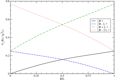
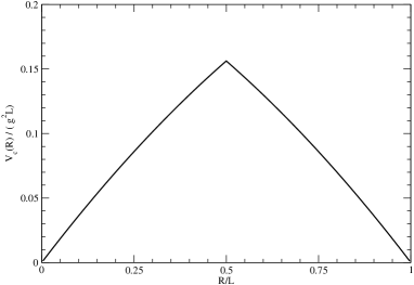
Figure 3: Left panel: The Coulomb Hamiltonian $V_{C}(z)$ for the four shortest Wilson states $|\,z\,\rangle$. Right panel: The true quark-antiquark potential for $D=1+1$ Yang-Mills theory on the spacetime cylinder, as extracted from the prescription eq. (40).

The final sum over energy eigenvalues $n$ in eq. (54) can only be performed numerically. At large spacetime volumes $LT\gg g^{-2}$, the ground state $n=0$ dominates the sum, and all remaining contributions are exponentially suppressed. The relevant matrix element $|\langle\,0\,|\,R\,\rangle|^{2}$ is then independent of $T$ and approaches unity for large space extensions $L\gg R$. This entails that

$$-\lim_{T\to\infty}T^{-1}\,\ln\,\mathrm{tr}\,\langle\,z\,|\,e^{-T(H-E_{0})}\,|\,z\,\rangle=V_{C}(z)\,,\qquad\qquad z\in\{R\,,R-L\}\,.$$

The prescription (40) (with only $m=0$ and $m=-1$ competing for the minimum if $|R|<L$) yields the final result

$$V(R)=\min_{m\in\{0,-1\}}\,V_{C}(R+mL)=\min_{m\in\{0,-1\}}\,\left[\frac{3}{8}g^{2}(R+mL)\,\left(1-\frac{1}{3}\frac{R+mL}{L}\right)\right]\,.$$ (56)

This function is plotted in the right panel of figure 3. It is symmetric around $R=L/2$ and thus invariant under the replacement $R\to L-R$. The previous construction also entails that $V(R)$ has to be extended periodically outside the range $0\leq R\leq L$, although we have not performed that calculation explicitly. The level crossing at $R=L/2$ is clearly visible, when the two Wilson states from figure 2 exchange their roles. The effective string tension is

$$\sigma_{1+1}\equiv\left.\frac{dV(R)}{dR}\right|_{R/L\to 0}=\frac{3}{8}\,g^{2}$$ (57)

and this agrees with eq. (38) and calculations using path integrals Witten (1991); Blau and Thompson (1992) or explicit quark wave functions Engelhardt and Schreiber (1995). In the infinite volume limit $L\to\infty$, the potential is exactly linear, since all Wilson states other than $|\,R\,\rangle$ have energy of order $\mathscr{O}(L)$ and thus decouple from the spectrum.

V Yang-Mills theory in $(3+1)$ dimensions

Let us finally address the most complex example, viz. non-Abelian Yang-Mills theory in $(3+1)$ dimensions. We employ again the first method based on the standard gauge fixed Hamiltonian eq. (24),

$$\langle W\rangle=\mathrm{tr}\,\langle\,\mathbf{R}^{\perp}\,|\,e^{-T(H-E_{0})}\,|\,\mathbf{R}\,\rangle=\int\mathscr{D}A^{\perp}\mathscr{J}[A^{\perp}]\,\Psi_{R}[\mathbf{A}^{\perp}]\,e^{-T(H-E_{0})}\,\Psi_{R}[\mathbf{A}^{\perp}]\,.$$ (58)

Here, $\mathscr{J}$ is the Faddeev-Popov determinant and $\Psi_{{\mbox{\boldmath$\scriptstyle{R}$\unboldmath}}}[\mathbf{A}^{\perp}]=\langle\,\mathbf{A}^{\perp}\,|\,U(\mathbf{R})\,|\,0\,\rangle$ is the wave function of the Wilson state $|\,\mathbf{R}\,\rangle$ in Coulomb gauge.

To proceed, we could take a model for the true Yang-Mills ground state in Coulomb gauge, $|\,0\,\rangle$ and compute $\Psi_{R}[\mathbf{A}^{\perp}]$ by application of the Wilson line. Below, we will instead apply an approximation where only the vev. of the Hamiltonian (rather than the full evolution operator) is required. In such cases, it is expedient to perform the same unitary transformation eq. (15) which transfers the Wilson line in the Hamiltonian, this time however with the gauge fixed version eq. (24) of the initial Hamiltonian. Retracing the steps that led from eq. (5) to eq. (17) with the parallel transporter $U(\mathbf{R})$ now depending on $\mathbf{A}^{\perp}$ only, we find that a transversal electric field $\mbox{\boldmath$\epsilon$\unboldmath}^{\perp}$ is induced which shifts the momentum operator in eq. (24). Moreover, the transformation of the Coulomb term eq. (25) replaces the full charge $(\rho+\rho_{\rm dyn})$ with $(\widetilde{\rho}+\rho_{\rm dyn}+\rho_{\rm ind})$, where $\widetilde{\rho}$ is the rotated external charge eq. (19), $\rho_{\rm dyn}\equiv-[\,\hat{\mathbf{A}}^{\perp}\,,\,\mbox{\boldmath$\Pi$\unboldmath}^{\perp}\,]$ and $\rho_{\rm ind}\equiv-[\,\hat{\mathbf{A}}^{\perp}\,,\,\mbox{\boldmath$\epsilon$\unboldmath}^{\perp}\,]$. The effective gauge fixed Hamiltonian is therefore

$$\widetilde{H}^{\rm fix}=H_{YM}^{\rm fix}+\tilde{V}_{C}+\Delta H\,,$$ (59)

where the first piece is just the usual gauge-fixed Hamiltonian in the absence of external charges,

$$H_{\rm YM}^{\rm fix} = \frac{g^{2}}{2}\,\int d^{3}x\,\mathscr{J}^{-1}\,\mbox{\boldmath$\Pi$\unboldmath}^{\perp}_{a}(\mathbf{x})\,\mathscr{J}\,\mbox{\boldmath$\Pi$\unboldmath}^{\perp}_{a}(\mathbf{x})+\frac{1}{2g^{2}}\,\int d^{3}x\,\big{[}\,\mathbf{B}^{a}(\mathbf{x})\,\big{]}^{2}+$$ (60)

$$\qquad\qquad{}+\frac{g^{2}}{2}\,\int d^{3}(x,y)\,\mathscr{J}^{-1}\,\rho^{a}_{\rm dyn}(\mathbf{x})\,\mathscr{J}\cdot F^{ab}(\mathbf{x},\mathbf{y})\,\rho_{\rm dyn}^{b}(\mathbf{y})\,\,.$$

The two additional pieces comprise a non-Abelian Coulomb potential

$$\widetilde{V}_{C}=\frac{g^{2}}{2}\int d^{3}(x,y)\,\widetilde{\rho}^{a}(\mathbf{x})\,F^{ab}(\mathbf{x},\mathbf{y})\,\widetilde{\rho}^{b}(\mathbf{y})$$ (61)

and a new contribution which contains the coupling of the external charges $\widetilde{\rho}$ to the dynamical charge of the gluon, as well as the terms induced by the electric field due to the Wilson line,

$$\Delta H = \frac{g^{2}}{2}\int d^{3}x\,\Big{\{}\mathscr{J}^{-1}\,\mbox{\boldmath$\Pi$\unboldmath}^{\perp}(\mathbf{x})\,\mathscr{J}\,\mbox{\boldmath$\epsilon$\unboldmath}^{\perp}(\mathbf{x})+\mbox{\boldmath$\epsilon$\unboldmath}^{\perp}(\mathbf{x})\,\mbox{\boldmath$\Pi$\unboldmath}^{\perp}(\mathbf{x})+\big{[}\,\mbox{\boldmath$\epsilon$\unboldmath}^{\perp}(\mathbf{x})\,\big{]}^{2}\Big{\}}+$$

$${}+\frac{g^{2}}{2}\,\int d^{3}(x,y)\,\Bigg{[}\mathscr{J}^{-1}\,\rho_{\rm dyn}\mathscr{J}\,F\,(\widetilde{\rho}+\rho_{\rm ind})+(\widetilde{\rho}+\rho_{\rm ind})\,F\,\rho_{\rm dyn}+$$

$$\qquad\qquad\qquad\qquad+\rho_{\rm ind}\,F\,\rho_{\rm ind}+\rho_{\rm ind}\,F\,\widetilde{\rho}+\widetilde{\rho}\,F\,\rho_{\rm ind}\Bigg{]}$$

While a full calculation of $\langle W\rangle$ cannot be done with a Hamiltonian as complicated as eq. (59), it naturally lends itself to approximations based on models for the (uncharged) vacuum wave functional, since the whole effect of the Wilson line is already incorporated in the dynamics, i.e. in the transformed Hamiltonian $\widetilde{H}$. In the following, we will sketch such an approximation based on a Gaussian model for the vacuum wave functional, as obtained recently by variational calculations Feuchter and Reinhardt (2004, 2004); Reinhardt and Feuchter (2005); Epple et al. (2007, 2008); Reinhardt and Schleifenbaum (2009); Schleifenbaum et al. (2006); Reinhardt and Epple (2007).

In a first step, we use Jensen’s inequality to obtain a lower bound for the Wilson loop (and thus an upper bound for the Wilson potential),

$$\langle\,W\,\rangle=\left\langle\,0\,\left|\,\mathrm{tr}\,e^{-T(\widetilde{H}^{\rm fix}-E_{0})}\,\right|\,0\,\right\rangle\geq\mathrm{tr}\,\exp\Big{[}-\left\langle\,0\,\left|\,T\,(\widetilde{H}^{\rm fix}-E_{0})\,\right|\,0\,\right\rangle\Big{]}\,.$$

The advantage of the rhs is that only the vev of the Hamiltonian is required. In particular, the eigenvalue equation $H_{\rm YM}^{\rm fix}\,|0\,\rangle=E_{0}\,|\,0\,\rangle$ entails that the YM Hamiltonian drops out and we are left with

$$\langle\,W\,\rangle\geq\mathrm{tr}\,\exp\left[-\left\langle\,0\,\left|\,T\,(\widetilde{V}_{C}+\Delta H)\,\right|\,0\,\right\rangle\right]\,.$$ (62)

To compute the exponent on the rhs of this equation, we write out $\Delta H$ explicitly,

$$\langle\,0\,|\,\widetilde{V}_{C}+\Delta H\,|\,0\,\rangle=\langle\,0\,|\,\widetilde{V}_{C}\,|\,0\,\rangle+\Big{\langle}\,0\,\Big{|}\,\frac{g^{2}}{2}\int\left(\mbox{\boldmath$\epsilon$\unboldmath}^{\perp}\mbox{\boldmath$\Pi$\unboldmath}^{\perp}+\mbox{\boldmath$\Pi$\unboldmath}^{\perp}\mbox{\boldmath$\epsilon$\unboldmath}^{\perp}+\mathscr{J}^{-1}\,[\,\mbox{\boldmath$\Pi$\unboldmath}^{\perp}\,,\,\mathscr{J}\,]\,\mbox{\boldmath$\epsilon$\unboldmath}^{\perp}+\big{[}\mbox{\boldmath$\epsilon$\unboldmath}^{\perp}\big{]}^{2}+\overline{\Delta H}\right)\,\Big{|}\,0\,\Big{\rangle}\,.$$

(The explicit form of the remainder $\overline{\Delta H}$ will be given below.) Next we neglect the commutators

$$[\,\mbox{\boldmath$\Pi$\unboldmath}^{\perp}\,,\,\mathscr{J}\,]\approx 0\,,\qquad\quad[\,U^{\perp}(\mathbf{R})\,,\,T^{a}\,]\approx 0$$ (63)

where $U^{\perp}(\mathbf{R})$ is the Wilson line $\mathbf{0}\to\mathbf{R}$ built from the transversal vector field $\mathbf{A}^{\perp}$. The first equation means that the gauge field dependence of the Faddeev–Popov determinant is neglected, $\mathscr{J}=\mbox{const}$, while the second equation discards the matrix structure of the non-Abelian parallel transporter, $U^{\perp}\sim\mathbbm{1}$. (This is stronger than just neglecting path ordering). As a consequence, the external charge and the induced electric field also become independent of the gauge field,

$$\widetilde{\rho}^{a}(\mathbf{x}) \to iT^{a}\,\big{[}\delta(\mathbf{x})-\delta(\mathbf{x}-\mathbf{R})\big{]}$$

$$\big{[}\epsilon^{\perp}\big{]}^{a}_{i}(\mathbf{x}) \to iT^{a}\int dy_{k}\,t_{ik}(\mathbf{x})\,\delta(\mathbf{x}-\mathbf{y})\,.$$ (64)

The relevant matrix element in the exponent of eq. (62) now reads

$$\langle\,0\,|\,\widetilde{V}_{C}+\Delta H\,|\,0\,\rangle\approx\frac{g^{2}}{2}\int\widetilde{\rho}\,\overline{F}\,\widetilde{\rho}+\frac{g^{2}}{2}\int d^{3}x\,\big{[}\mbox{\boldmath$\epsilon$\unboldmath}^{\perp}_{a}(\mathbf{x})\big{]}^{2}+\langle\,0\,|\,\overline{\Delta H}\,|\,0\,\rangle$$ (65)

where we used global color and translation invariance to infer the structure

$$\langle\,0\,|\,\mbox{\boldmath$\Pi$\unboldmath}^{\perp}_{a}(\mathbf{x})\,|\,0\,\rangle=0\,,\qquad\qquad\langle\,0\,|\,F^{ab}(\mathbf{x},\mathbf{y})\,|\,0\,\rangle=\delta^{ab}\,\overline{F}(\mathbf{x}-\mathbf{y})\,.$$ (66)

The first term on the rhs of eq. (65) is the non-Abelian Coulomb interaction, i.e. the remaining terms describe, within our approximation scheme, the difference between the (non-Abelian) Coulomb potential and the Wilson potential. We will now investigate these corrections:

The third term on the rhs of eq. (65) involves the coupling of the various charges via the Coulomb kernel,

$$\overline{\Delta H}=\frac{g^{2}}{2}\int\Big{[}\mathscr{J}^{-1}\rho_{\rm dyn}\mathscr{J}F\left(\tilde{\rho}+\rho_{\rm ind}\right)+\left(\tilde{\rho}+\rho_{\rm ind}\right)\,F\,\rho_{\rm dyn}+\rho_{\rm ind}\,F\,\rho_{\rm ind}+\rho_{\rm ind}\,F\,\tilde{\rho}+\tilde{\rho}\,F\,\rho_{\rm ind}\Big{]}\hskip 2.84544pt.$$ (67)

Its vev is still too complex for a direct evaluation. To further simplify it, we make yet another approximation and assume that the Coulomb kernel, $F$, inside charge interactions can be replaced by its vev eq. (66). In an obvious notation, this means

$$\langle\,0\,|\,Q^{a}\,F^{ab}\,Q^{\prime b}\,|\,0\rangle\approx\langle\,0\,|\,Q^{a}\,Q^{\prime b}\,|\,0\,\rangle\cdot\langle\,0\,|\,F^{ab}\,|\,0\,\rangle=\langle\,0\,|\,Q^{a}\,Q^{\prime a}\,|\,0\,\rangle\cdot\overline{F}$$ (68)

for any two operators $Q,Q^{\prime}$. We can now use the previous approximation eq. (63) and consequently eq. (64) to put $\langle\,0\,|\,\overline{\Delta H}\,|\,0\rangle\,$ in the form

$$\frac{g^{2}}{2}\int\Big{[}\,\langle\rho_{\rm dyn}\rangle\,\overline{F}\,\widetilde{\rho}+\langle\rho_{\rm dyn}\,\rho_{\rm ind}\rangle\,\overline{F}+\widetilde{\rho}\,\overline{F}\,\langle\rho_{\rm dyn}\rangle+\langle\rho_{\rm ind}\,\rho_{\rm dyn}\rangle\,\overline{F}+\langle\rho_{\rm ind}\,\rho_{\rm ind}\rangle\,\overline{F}+\langle\rho_{\rm ind}\rangle\,\overline{F}\,\widetilde{\rho}+\widetilde{\rho}\,\overline{F}\,\langle\rho_{\rm ind}\rangle\,\Big{]}\,.$$

Since Coulomb gauge does not single out a color or space direction, global color and translation invariance tells us that

$$\langle\,0\,|\,\mathbf{A}^{\perp}_{a}(\mathbf{x})\,|\,0\,\rangle=0\,,\qquad\qquad\langle\,0\,|\,\mathbf{A}^{\perp}_{a}(\mathbf{x})\,\mbox{\boldmath$\Pi$\unboldmath}^{\perp}_{b}(\mathbf{x})\,|\,0\,\rangle\sim\delta_{ab}$$

so that $\langle\rho_{\rm dyn}\rangle=\langle\rho_{\rm ind}\rangle=0$. Furthermore, we have the charge correlator

$$\langle\,\rho_{\rm dyn}\,\rho_{\rm ind}\,\rangle=\langle\,\rho_{\rm ind}\,\rho_{\rm dyn}\,\rangle=\epsilon_{k}^{\perp\,a}(\mathbf{x})\,\langle\,0\,|\,f^{abe}\,f^{edc}\,\mathbf{A}_{k}^{\perp\,b}(\mathbf{x})\,\mathbf{A}_{i}^{\perp\,c}(\mathbf{x})\,\mbox{\boldmath$\Pi$\unboldmath}^{\perp\,d}_{i}(\mathbf{x})\,|\,0\,\rangle\,.$$

(For the first equality, we have to commute $\Pi$ to the right and use $\langle\mathbf{A}\rangle=0$.) The vev is a single component of a color and space vector, and again global color and (spatial) rotation invariance tells us that it has to vanish. We are thus left with only a single term

$$\langle\,0\,|\,\overline{\Delta H}\,|\,0\,\rangle=\frac{g^{2}}{2}\,f^{abc}\,f^{ade}\int d^{3}(x,y)\,\epsilon_{i}^{\perp\,b}(\mathbf{x})\,\epsilon_{k}^{\perp\,d}(\mathbf{x})\,\overline{F}(\mathbf{x}-\mathbf{y})\cdot\langle\,0\,|\,A_{i}^{\perp\,c}(\mathbf{x})\,A_{k}^{\perp\,e}(\mathbf{y})\,|\,0\,\rangle\,.$$

Using global color and translation invariance one last time, the gluon propagator must take the form

$$\langle\,0\,|\,A_{i}^{\perp\,c}(\mathbf{x})\,A_{k}^{\perp\,e}(\mathbf{y})\,|\,0\,\rangle=\delta^{ce}\,t_{ik}(\mathbf{x})\,D(|\mathbf{x}-\mathbf{y}|)$$ (69)

with an unknown scalar function $D(r)$. Thus eventually, with $f^{abc}\,f^{adc}=N_{C}\,\delta^{bd}$,

$$\langle\,0\,|\,\overline{\Delta H}\,|\,0\,\rangle=\frac{g^{2}}{2}\,N_{C}\int\mbox{\boldmath$\epsilon$\unboldmath}^{\perp}_{a}(\mathbf{x})\,\overline{F}(\mathbf{x}-\mathbf{y})\,D(\mathbf{x}-\mathbf{y})\,\mbox{\boldmath$\epsilon$\unboldmath}^{\perp}_{a}(\mathbf{y})\,.$$ (70)

We observe that this expression can be combined with the second term in eq. (65).

The first term in eq. (65) is the non-Abelian Coulomb interaction. It can easily be computed within our approximation scheme, since the simplified form eq. (64) for the external charge implies

$$\langle\,0\,|\,\widetilde{V}_{C}\,|\,0\,\rangle=\frac{g^{2}}{2}\int\widetilde{\rho}\,\overline{F}\,\widetilde{\rho}=-\frac{g^{2}}{2}\,C_{2}\Big{[}\,\overline{F}(R)-\overline{F}(0)\,\Big{]}$$ (71)

with the quadratic Casimir $C_{2}(N_{c})=-\sum_{a}\,T^{a}\,T^{a}$. Putting everything together, we arrive at

$$\langle\,W\,\rangle \approx \exp\Bigg{\{}-T\,\frac{g^{2}}{2}\,N_{C}\int d^{3}(x,y)\,\mbox{\boldmath$\epsilon$\unboldmath}_{a}^{\perp}(\mathbf{x})\,\Big{[}\,N_{C}^{-1}\,\delta(\mathbf{x}-\mathbf{y})+\overline{F}(\mathbf{x}-\mathbf{y})\,D(\mathbf{x}-\mathbf{y})\Big{]}\,\mbox{\boldmath$\epsilon$\unboldmath}_{a}^{\perp}(\mathbf{y})\Bigg{\}}\times$$ (72)

$${}\times\exp\Bigg{\{}-T\,C_{2}\,g^{2}\,\Big{[}\overline{F}(R)-\overline{F}(0)\,\Big{]}\,\Bigg{\}}\,.$$

To estimate the contribution from the first line, we require some dynamical input on the gluon propagator $D$ and the Coulomb kernel $\overline{F}$. (Within our approximation, this is the only place where the actual form of the vacuum wave functional enters.) The exact analytical expressions are unknown, but we have reliable data from recent variational calculations Feuchter and Reinhardt (2004, 2004); Reinhardt and Feuchter (2005); Epple et al. (2007, 2008); Reinhardt and Schleifenbaum (2009); Schleifenbaum et al. (2006); Reinhardt and Epple (2007), which are also in decent agreement with high precision lattice measurements Quandt et al. (2007); Burgio et al. (2009). The latter give

$$D(k) = \frac{1}{2\,\omega(k)}\,,\qquad\qquad\omega(k)\approx\sqrt{k^{2}+M^{4}/k^{2}}$$

$$\overline{F}(k) \simeq 8\pi\,\frac{\sigma_{C}}{k^{4}}\,,\qquad\qquad k\to 0\,,$$ (73)

where $M\approx 880\,\mathrm{MeV}$ is the Gribov mass and $\sigma_{C}$ is the Coulomb string tension, which is about $2\ldots 3$ times the Wilson string tension.

With this input, it is shown in appendix B that the integral in the first line of eq. (72) yields a Coulomb type of potential which decays as $1/R$ at large distances and is thus subleading as compared to the second line (which gives a linearly rising potential). Thus,

$$\langle\,W\,\rangle\approx\mathrm{const}\cdot\exp\Big{\{}\,-T\,C_{2}\,g^{2}\,\overline{F}(R)+\mathrm{subleading}\Big{\}}$$ (74)

and the Wilson string tension equals the Coulomb string tension.

This simple result should, however, be taken with some caution: In deriving it, we had to make a number of approximations,

1. Jensen’s inequality eq. (62)

2. the commutator approximations eq. (63)

3. the factorization eq. (68)

4. the variational solutions for the Green functions $D(r)$ and $\overline{F}(\mathbf{x})\,$

The corresponding errors are not all under good control: While lattice calculations indicate that the variational solutions in item #4 are close to the exact results, Jensen’s inequality #1 entails that our potential is, a priori, only an upper bound to the true Wilson potential, and it is hard to predict the quality of that bound. Even more severe is the factorization #3, since it causes most of the couplings between the various charges to vanish. In particular, we have lost the coupling of the external charges at the end points of the Wilson lines with the dynamical charges of the gluon, as described by the contribution

$$\frac{g^{2}}{2}\int\Big{[}\mathscr{J}^{-1}\rho_{\rm dyn}\mathscr{J}F\,\widetilde{\rho}+\widetilde{\rho}\,F\,\rho_{\rm dyn}\Big{]}\hskip 2.84544pt.$$ (75)

In perturbation theory, one can show explicitly that this term reduces the Coulomb potential $\frac{1}{2}\,g^{2}\int\rho\,F\,\rho$. It is tempting to expect that eq. (75) will screen the Coulomb interaction when treated non-perturbatively, and that this effect provides the major reduction of the Coulomb string tension to the Wilsonian one. A detailed study of the screening of external color charges by dynamical gluons is subject to ongoing research.

VI Conclusions

In this paper, we have investigated the temporal Wilson loop in the Hamiltonian formulation of Yang-Mills theory. Using a unitary transformation we have demonstrated that the effect of the Wilson lines is to introduce a new non-Abelian (field-dependent) electric field in the Hamiltonian. This formulation leads to the correct result in some simple cases where the exact gauge-invariant ground state is known.

Without the exact ground state at hand, we need to fix the gauge, for which Coulomb gauge is a particularly useful choice: Since the only constraint on physical states is Gauss’ law which can be resolved exactly, any normalizable Ansatz for the ground state wave functional is admissible and the formulation is ideal for variational approaches. We have shown how to treat the exactly solvable cases in Coulomb gauge, and applied these methods to the physically important case of Yang-Mills theory in $(3+1)$ dimensions using the optimal Gaussian wave functional from recent variational approaches as input. Unfortunately, the dynamics of the system was still too complex so that additional approximations were necessary to find an analytical result. Within these approximation, the Wilson string tension was found to match the Coulomb string tension, $\sigma\approx\sigma_{c}$. Finally, we have discussed the qualitative effect of the neglected couplings in the Hamiltonian, which are expected to suppress the Wilson string tension towards the value $\sigma/\sigma_{c}\simeq 0.3\,\ldots\,0.5$ favored by lattice simulations. A closer investigation of those missing couplings is currently underway.

Appendix A The Abelian Coulomb potential in spherical coordinates

It is convenient to use spherical coordinates $\mathbf{x}=(r,\hat{x}),\mathbf{R}=(R,\hat{\mathbf{R}})$ and express the $\delta$-function by

$$\delta(\mathbf{x}-s\mathbf{R})=\frac{\delta(r-sR)}{r^{2}}\sum\limits_{l,m}Y^{*}_{lm}(\hat{x})Y_{lm}(\hat{R})\hskip 2.84544pt.$$ (76)

With this representation we find with (20)

$$\frac{g^{2}}{2}\int d^{3}x\,\mbox{\boldmath$\epsilon$\unboldmath}(\mathbf{x})^{2} = \frac{g^{2}}{2}R^{2}\int\limits^{1}_{0}ds\int\limits^{1}_{0}ds^{\prime}\int\limits^{\infty}_{0}drr^{2}\frac{\delta(r-sR)}{r^{2}}\frac{\delta(r-s^{\prime}R)}{r^{2}}\times$$ (77)

$${}\times\sum\limits_{lm}\sum\limits_{l^{\prime}m^{\prime}}\int d\Omega_{x}Y^{*}_{lm}(\hat{x})Y_{l^{\prime}m^{\prime}}(\hat{x})Y_{lm}(\hat{R})Y^{*}_{l^{\prime}m^{\prime}}(\hat{R})\hskip 2.84544pt.$$

Performing the integrals over $r,s^{\prime}$ and $\Omega_{x}$ by means of the orthonormality of $Y_{lm}(\hat{x})$ we obtain

$$\frac{g^{2}}{2}\int d^{3}x\,\mbox{\boldmath$\epsilon$\unboldmath}(\mathbf{x})^{2}=\frac{g^{2}}{2}\frac{1}{R}\int\limits^{1}_{0}\frac{ds}{s^{2}}\,\delta^{(2)}_{\sphericalangle}(\hat{0})\hskip 2.84544pt,$$ (78)

where $\delta^{(2)}_{\sphericalangle}$ is defined by

$$\delta^{(2)}_{\sphericalangle}(\Omega-\Omega^{\prime})=\sum\limits_{lm}Y^{*}_{lm}(\hat{\Omega})Y_{lm}(\Omega^{\prime})=\delta(\cos\vartheta-\cos\vartheta^{\prime})\delta(\varphi-\varphi^{\prime})\hskip 2.84544pt.$$ (79)

Note that $\delta^{(2)}_{\sphericalangle}(\hat{\Omega})$ is dimensionless. From the final integral

$$\left.\int\limits^{1}_{0}\frac{ds}{s^{2}}=-\frac{1}{s}\right|^{1}_{s=0}=-1+\infty$$ (80)

we ignore the divergent contribution from the lower integration limit, which represents the self-energy contribution of the two charges. The divergent factor $\delta^{(2)}_{\sphericalangle}(\hat{0})$ has a different origin: it is due to the infinitely thin Wilson line between the charges and gives rise to the renormalization of the Wilson loop operator, cf. eq. (33). In the present context, this amounts to the renormalization of the bare charge,

$$g^{2}\,\delta^{(2)}_{\sphericalangle}(\hat{0})=\frac{e^{2}}{4\pi}\hskip 2.84544pt,$$ (81)

so that the Coulomb potential from eq. (78) becomes eventually

$$V(R)=\frac{g^{2}}{2}\int d^{3}x\,\mbox{\boldmath$\epsilon$\unboldmath}(\mathbf{x})^{2}=-\frac{e^{2}}{4\pi R}\hskip 2.84544pt.$$ (82)

Our result (78) disagrees with the similar calculation in ref. Gaete (1999), where the divergent factor $\delta^{(2)}_{\sphericalangle}(\hat{0})$ is replaced by $1/(4\pi)$, so that no renormalization seems necessary (except for the subtraction of the self-energy).

To relate the present calculation to our reasoning in section II.1 of the main text, it should be noted that eq. (76) implies $s=r/R=|\mathbf{x}|/R$ and the lower bound $s=0$ in eq. (80) should therefore be $s_{\rm min}=|\mathbf{x}|_{\rm min}/R$, with $|\mathbf{x}|_{\rm min}$ a minimal distance of the two charges. If we put a cutoff $s_{\rm min}=a/R$ for the lower integration limit in eq. (80), the (unrenormalized) potential becomes

$$V(R)=-\frac{g^{2}}{2}\,\delta^{(2)}_{\sphericalangle}(\hat{0})\,\left(\frac{1}{R}-\frac{1}{a}\right)\,.$$

Clearly, the self-energy of the charges corresponds to the second term in the parenthesis. However, even with a minimal distance cutoff $a>0$, there is still a divergent prefactor coming from the infinitely thin Wilson line. To see this, recall that $\mbox{\boldmath$\epsilon$\unboldmath}(\mathbf{x})$ has support on the Wilson line only, so that $\hat{\mathbf{x}}=\hat{\mathbf{R}}$ if the Wilson line is infinitely thin, and hence the argument of the angular delta-function $\delta^{(2)}_{\sphericalangle}$ in eq. (78) vanishes. The divergent prefactor is thus well understood as a typical OPE divergence for the thin Wilson line which involves field operators $\mathbf{A}(\mathbf{x})$ at arbitrarily close positions. It must be absorbed in the multiplicative renormalization $Z_{W}$ of the Wilson loop operator, cf. the discussion following eq. (33) in the main text.

Appendix B Contribution of $\mbox{\boldmath$\epsilon$\unboldmath}^{\perp}$ to the Coulomb potential

To estimate the role of $\mbox{\boldmath$\epsilon$\unboldmath}^{\perp}$ we calculate the vacuum expectation value of the induced Coulomb term

$$\Delta H^{(1)}_{c}=\frac{g^{2}}{2}\int\hat{\mathbf{A}}\cdot\mbox{\boldmath$\epsilon$\unboldmath}^{\perp}F\hat{\mathbf{A}}\cdot\mbox{\boldmath$\epsilon$\unboldmath}^{\perp}\hskip 2.84544pt.$$ (83)

Using the approximation

$$\langle\hat{A}F\hat{A}\rangle\simeq\langle\hat{A}\hat{A}\rangle\langle F\rangle\equiv\frac{\overline{F}}{2\omega}$$ (84)

and ignoring the path ordering in $\mbox{\boldmath$\epsilon$\unboldmath}^{\perp}(x)$, i.e. $\widetilde{T}_{a}(x)\simeq T_{a}$, we obtain

$$\langle\Delta H^{(1)}_{c}\rangle=C_{2}\,\frac{g^{2}}{2}\int\limits^{\mbox{\boldmath$\scriptstyle R$\unboldmath}}_{0}dx_{i}\int\limits^{\mbox{\boldmath$\scriptstyle R$\unboldmath}}_{0}dy_{j}\,t_{ij}(x)\omega^{-1}(x,y)\,\overline{F}(x,y)\hskip 2.84544pt,$$ (85)

where $C_{2}\,\mathbbm{1}=-T_{a}\,T_{a}$ is the quadratic Casimir operator in the color representation of the Wilson loop. Putting the path along the $z$-axis from $0$ to $R$

$$x_{i}=\delta_{i3}Rs\hskip 2.84544pt,\qquad\hskip 2.84544pty_{i}=\delta_{i3}Rt$$ (86)

we find after Fourier transformation and using spherical coordinates in momentum space

$$\langle\Delta H^{(1)}_{c}\rangle = R^{2}\left(\frac{1}{2\pi}\right)^{4}\int\limits^{\infty}_{0}\frac{dkk^{2}}{\omega(k)}\int\limits^{\infty}_{0}dp\,p^{2}F(p)\int\limits^{1}_{0}ds\int\limits^{1}_{0}dt\times$$ (87)

$${}\times\int\limits^{1}_{-1}dz\,(1-z^{2})e^{izkR(s-t)}\int\limits^{1}_{-1}dz^{\prime}\,e^{iz^{\prime}pR(s-t)}\,.$$

We are interested in the large $R$ behavior of this quantity. Assuming the usual IR-behavior of the Green functions,

$$\omega(k)\sim\frac{1}{k}\hskip 2.84544pt,\qquad\overline{F}(k)\sim\frac{1}{k^{4}}$$ (88)

as $k\to 0$, and furthermore introducing dimensionless variables

$$\bar{k}=kR\hskip 2.84544pt,\qquad\bar{p}=pR\,,$$ (89)

on finds

$$\langle\Delta H^{(1)}_{c}\rangle\sim\frac{1}{R}\hskip 2.84544pt\qquad\quad\mbox{as\quad}R\to\infty\hskip 2.84544pt.$$ (90)

This quantity is therefore subleading at large distances and hence irrelevant for the screening of the Coulomb string tension.

References

- Zwanziger (2003) D. Zwanziger, Phys.Rev.Lett., 90, 102001 (2003), arXiv:hep-lat/0209105 [hep-lat] .
- Langfeld and Moyaerts (2004) K. Langfeld and L. Moyaerts, Phys.Rev., D70, 074507 (2004), arXiv:hep-lat/0406024 [hep-lat] .
- Quandt et al. (2007) M. Quandt, G. Burgio, S. Chimchinda, and H. Reinhardt, PoS, LAT2007, 325 (2007), arXiv:0710.0549 [hep-lat] .
- Voigt et al. (2007) A. Voigt, E.-M. Ilgenfritz, M. Muller-Preussker, and A. Sternbeck, PoS, LAT2007, 338 (2007), arXiv:0709.4585 [hep-lat] .
- Voigt et al. (2008) A. Voigt, E.-M. Ilgenfritz, M. Muller-Preussker, and A. Sternbeck, Phys.Rev., D78, 014501 (2008), arXiv:0803.2307 [hep-lat] .
- Burgio et al. (2009) G. Burgio, M. Quandt, and H. Reinhardt, Phys.Rev.Lett., 102, 032002 (2009), arXiv:0807.3291 [hep-lat] .
- Burgio et al. (2010) G. Burgio, M. Quandt, and H. Reinhardt, Phys.Rev., D81, 074502 (2010), arXiv:0911.5101 [hep-lat] .
- Quandt et al. (2010) M. Quandt, H. Reinhardt, and G. Burgio, Phys.Rev., D81, 065016 (2010), arXiv:1001.3699 [hep-lat] .
- Gribov (1978) V. Gribov, Nucl.Phys., B139, 1 (1978).
- Zwanziger (1997) D. Zwanziger, Nucl.Phys., B485, 185 (1997), arXiv:hep-th/9603203 [hep-th] .
- Burgio et al. (2000) G. Burgio, R. De Pietri, H. Morales-Tecotl, L. Urrutia, and J. Vergara, Nucl.Phys., B566, 547 (2000), arXiv:hep-lat/9906036 [hep-lat] .
- Szczepaniak and Swanson (2002) A. P. Szczepaniak and E. S. Swanson, Phys.Rev., D65, 025012 (2002), arXiv:hep-ph/0107078 [hep-ph] .
- Feuchter and Reinhardt (2004) C. Feuchter and H. Reinhardt, Phys.Rev., D70, 105021 (2004a), arXiv:hep-th/0408236 [hep-th] .
- Feuchter and Reinhardt (2004) C. Feuchter and H. Reinhardt, (2004b), arXiv:hep-th/0402106 [hep-th] .
- Reinhardt and Feuchter (2005) H. Reinhardt and C. Feuchter, Phys.Rev., D71, 105002 (2005), arXiv:hep-th/0408237 [hep-th] .
- Epple et al. (2007) D. Epple, H. Reinhardt, and W. Schleifenbaum, Phys.Rev., D75, 045011 (2007), arXiv:hep-th/0612241 [hep-th] .
- Epple et al. (2008) D. Epple, H. Reinhardt, W. Schleifenbaum, and A. Szczepaniak, Phys.Rev., D77, 085007 (2008), arXiv:0712.3694 [hep-th] .
- Reinhardt and Schleifenbaum (2009) H. Reinhardt and W. Schleifenbaum, Annals Phys., 324, 735 (2009), * Temporary entry *, arXiv:0809.1764 [hep-th] .
- Schleifenbaum et al. (2006) W. Schleifenbaum, M. Leder, and H. Reinhardt, Phys.Rev., D73, 125019 (2006), arXiv:hep-th/0605115 [hep-th] .
- Reinhardt and Epple (2007) H. Reinhardt and D. Epple, Phys.Rev., D76, 065015 (2007), arXiv:0706.0175 [hep-th] .
- Reinhardt (2008) H. Reinhardt, Phys.Rev.Lett., 101, 061602 (2008), arXiv:0803.0504 [hep-th] .
- Pak and Reinhardt (2009) M. Pak and H. Reinhardt, Phys.Rev., D80, 125022 (2009), arXiv:0910.2916 [hep-th] .
- Erickson et al. (2000) J. Erickson, G. Semenoff, R. Szabo, and K. Zarembo, Phys.Rev., D61, 105006 (2000), arXiv:hep-th/9911088 [hep-th] .
- Haagensen and Johnson (1997) P. E. Haagensen and K. Johnson, (1997), arXiv:hep-th/9702204 [hep-th] .
- Gaete (1999) P. Gaete, Phys.Rev., D59, 127702 (1999), arXiv:hep-th/9812245 [hep-th] .
- Heinzl et al. (2008) T. Heinzl, A. Ilderton, K. Langfeld, M. Lavelle, W. Lutz, et al., Phys.Rev., D77, 054501 (2008a), arXiv:0709.3486 [hep-lat] .
- Heinzl et al. (2008) T. Heinzl, A. Ilderton, K. Langfeld, M. Lavelle, W. Lutz, et al., Phys.Rev., D78, 034504 (2008b), arXiv:0806.1187 [hep-lat] .
- Christ and Lee (1980) N. Christ and T. Lee, Phys.Rev., D22, 939 (1980).
- Collins (1984) J. C. Collins, RENORMALIZATION. AN INTRODUCTION TO RENORMALIZATION, THE RENORMALIZATION GROUP, AND THE OPERATOR PRODUCT EXPANSION (Cambridge University Press, Cambridge, UK, 1984).
- Gervais and Neveu (1980) J.-L. Gervais and A. Neveu, Nucl.Phys., B163, 189 (1980).
- Polyakov (1980) A. M. Polyakov, Nucl.Phys., B164, 171 (1980).
- Witten (1991) E. Witten, Commun.Math.Phys., 141, 153 (1991).
- Blau and Thompson (1992) M. Blau and G. Thompson, Int.J.Mod.Phys., A7, 3781 (1992).
- Hetrick (1994) J. E. Hetrick, Nucl.Phys.Proc.Suppl., 34, 805 (1994), arXiv:hep-lat/9312012 [hep-lat] .
- Engelhardt and Schreiber (1995) M. Engelhardt and B. Schreiber, Z.Phys., A351, 71 (1995).