LTP and LISA
or: “look how far we have to go just to please Herr Einstein!”

Introduction and structure

This thesis addresses the problem of interferometer-based gravitational wave (GW) detection in space. The problem of detecting GW and decoupling them from the static gravitational background is an intricate one and can be viewed at least as a three-fold issue:

1. it implies a careful definition of a reference system. It is necessary to build a set of clocks and rulers in space to unequivocally measure radiative space-time variation of the Riemann tensor embedding the metric;

2. it demands the use of a detector. Pairs of particles in free-fall are the only reliable probe in this case, and then it is the ability of defining free-fall and detecting residual acceleration which need to be discussed carefully;

3. it calls for detailed knowledge of noise versus sensitivity, not to miss the wave signal or mistake noise for a signal.

The European Space Agency (ESA) and the National Aeronautics and Space Administration (NASA) are planning the Laser Interferometer Space Antenna (LISA) mission in order to detect GW. The need of accurate testing of free-fall and knowledge of noise in a space environment similar to LISA’s is considered mandatory a pre-phase for the project and therefore the LISA Pathfinder on the Small Mission for Advanced Research in Technology 2 (SMART-2) has been designed by ESA to fly the LISA Technology Package (LTP).

LTP will be blind to GW. By design, in order to detect any other disturbance which could jeopardise LISA’s sensitivity to GW themselves. Its goal will be to test free-fall by measuring the residual acceleration between two test-bodies in the dynamical scheme we address as “drag-free”, where the satellite is weakly coupled to one of the proof bodies and follows the motion of the other. The satellite is supposed to act as a shield to external disturbances and not to introduce too much noise by its internal devices. The spectral map of the residual acceleration as function of frequency will convey information on the local noise level, thus producing a picture of the environmental working conditions of LISA itself.

We’re going to show the following:

1. that construction of a freely-falling global reference frame is possible in theoretical terms, and laser detection is the utmost sensitive tool both for seeing GW - given a large baseline detector - and for mapping residual accelerations and noise (with a short baseline);

2. that a dedicated experiment can be designed fully by means of Newtonian mechanics and control theory. Carefully studied signals will be built as time-estimators of gauge-invariant observables;

3. that it just won’t be enough to send a probe to naîvely measure correlators of distance variation in outer space and deduce a spectral figure. It is necessary to design and project noise shapes, make educated “guesses” of spectra spelling all possible sources, carefully sum them to obtain overall estimates.

The description and contributions to the former tasks will be distributed as follows in the present thesis.

Chapter 1 starts from simple theoretical arguments and tries to clarify the idea of rulers and clocks as markers of $4$-locations in $4$-dimensional space-time. Using only Lorentz group local generators, we’ll show an absolute ruler may be built between two fiduciary mirrors out of a laser beam and that the phase variation $\Delta\theta_{\text{laser}}(t)$ of the laser light path is an unbiased estimator of the GW strain as:

$$\frac{\operatorname{d}\Delta\theta_{\text{laser}}(t)}{\operatorname{d}t}\simeq\frac{\pi c}{\lambda_{\text{laser}}}\left(h(t)-h\left(t-\frac{2L}{c}\right)\right)\,,$$ (1)

which is valid to $O\left(\omega_{\text{GW}}^{2}\right)$ where $\omega_{\text{GW}}$ is the GW pulsation, $h(t)$ the GW strain and $L$ is the detector baseline. $\lambda_{\text{laser}}$ is the laser wavelength and $c$ is the speed of light in vacuo.

We’ll shift to power spectral density (PSD) representation and describe the main sources of noise which can deceive this “interferometric eye”. Free-fall is replaced by drag-free and motivations are discussed. The final outcome of the chapter will be an estimate of the precision needed by the LISA detector in terms of the residual acceleration quality, which we may hereby summarise as:

$$\begin{split}S^{\nicefrac{{1}}{{2}}}_{\nicefrac{{\Delta F}}{{m}},\text{LISA}}(\omega)=&\sqrt{2}\times 3\times 10^{-15}\left(1+\left(\frac{\omega}{2\pi\times 3\,\mathrm{mHz}}\right)^{4}\right)^{\nicefrac{{1}}{{2}}}\,\nicefrac{\mathrm{m}}{\mathrm{s^{2}\sqrt{Hz}}}\,\\ \simeq&\sqrt{2}\times 3\times 10^{-15}\,\nicefrac{\mathrm{m}}{\mathrm{s^{2}\sqrt{Hz}}}\,@\,1\,\mathrm{mHz}\,,\end{split}$$ (2)

a picture of this is shown in figure 1 together with the interferometer acceleration noise. The LISA mission aims at revealing GWs by employing high-precision interferometer detection in space. Its Pathfinder will be a technology demonstrator to test free-fall and our knowledge of acceleration noise. The chapter ends with a thorough description of both and with a simplified uni-dimensional drag-free model to illustrate the features of the main interferometer measure channel and the physical discussion of measure modes.

LTP sensitivity is worsened by roughly a factor of $7$ with respect to the LISA goal, the measured acceleration will be differential and this is likely to be a worst case since the residual forces on the test-masses are considered as correlated over a short baseline:

$$S^{\nicefrac{{1}}{{2}}}_{\nicefrac{{\Delta F}}{{m}},\text{LTP}}(\omega)=3\times 10^{-14}\left(1+\left(\frac{\omega}{2\pi\times 3\,\mathrm{mHz}}\right)^{4}\right)^{\nicefrac{{1}}{{2}}}\,\nicefrac{\mathrm{m}}{\mathrm{s^{2}\sqrt{Hz}}}\,.$$ (3)

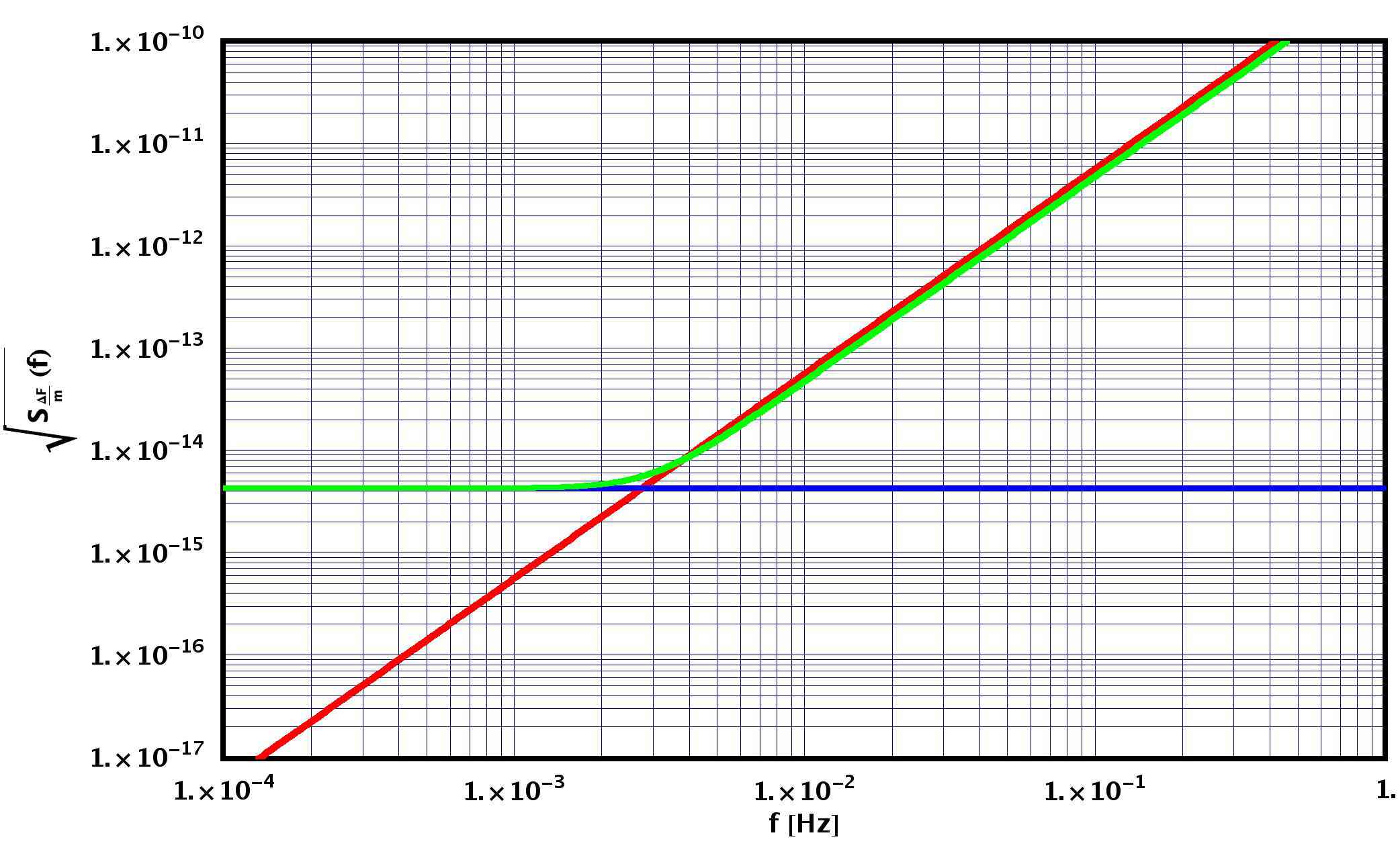
Figure 1: Noise PSDs in $\nicefrac{{\Delta F}}{{m}}$ for forces difference (blue), interferometer (red) and relaxed noise requirement of forces difference (green). Green line represents LISA’s targeted sensitivity.

Chapter 2 will complicate the simple mechanical model of chapter 1 and build the LTP dynamics from the ground up. Newtonian dynamics is employed to write down the equations of motion for the test-masses (TMs) and spacecraft (SC), with the purpose of deducing the dynamical behaviour of position/attitude variables and introduce the relative signal estimators. Controls, operating modes and limiting forms of signals are evaluated, their properties discussed and graphical behaviour sketched. The chapter is a mandatory deduction to connect the figures of chapter 1 with the world of noise in chapter 3. As we said, only the laser phase is regarded as the observable mapping the gauge-invariant Riemann variation into a distance fluctuation. The main interferometer signal, whose property we will derive in this chapter looks like:

$$\begin{split}\text{IFO}\left(x_{2}-x_{1}\right)\simeq\frac{1}{\omega_{\text{lfs},x}^{2}-\omega^{2}}\Bigl{(}&g_{2,x}-g_{1,x}-\text{IFO}_{n}(x_{1})\omega^{2}+(\delta x_{2}-\delta x_{1})\omega_{\text{p},2}^{2}+\\ &+\left(\omega_{\text{p},2}^{2}-\omega_{\text{p},1}^{2}\right)\left(\text{IFO}_{n}(x_{1})+\frac{g_{\text{SC},x}+z_{0}g_{\text{SC},\eta}}{\omega^{2}_{\text{df},x}}\right)\Bigr{)}\,,\end{split}$$ (4)

where residual local accelerations are marked with the letter $g$, stiffness with $\omega_{\text{p},i}^{2}$, deformations as ${\delta}x_{i}$. Noise in readout is embedded in the term $\text{IFO}_{n}(x_{1})$ while the terms $\omega_{\text{df}}^{2}$ and $\omega_{\text{lfs}}^{2}$ are drag-free (DF) and low-frequency suspension (LFS) transfer functions. The former signal carries the information we want, as:

$$\begin{split}S_{\nicefrac{{\Delta F}}{{m}}}^{\nicefrac{{1}}{{2}}}&=\frac{\omega^{2}}{m}S_{\Delta x}^{\nicefrac{{1}}{{2}}}\simeq\frac{\omega^{2}}{m}S_{\text{IFO}\left(\Delta x\right)}^{\nicefrac{{1}}{{2}}}=\\ &\simeq\frac{\omega^{2}}{m}\frac{\lambda_{\text{laser}}}{2\pi}S_{\text{IFO}\left(\Delta\phi_{\text{laser}}\right)}^{\nicefrac{{1}}{{2}}}\simeq\frac{\omega^{2}}{\omega_{\text{lfs},x}^{2}-\omega^{2}}S_{{\Delta}g_{x}}^{\nicefrac{{1}}{{2}}}\underset{\omega_{\text{lfs},x}^{2}\ll\omega^{2}}{\simeq}S_{{\Delta}g_{x}}^{\nicefrac{{1}}{{2}}}\,,\end{split}$$ (5)

where we denoted the difference of acceleration on the TMs along $\hat{x}$ with the symbol ${\Delta}g_{x}$. It is a very important step to impose the laser mapping in order to guarantee that a gauge-invariant measure is performed. This very signal is valid for mapping $\nicefrac{{{\Delta}F}}{{m}}$ on LTP but also for detecting a wave-strain $\nicefrac{{{\Delta}L}}{{L}}$ on a long-baseline interferometer mission such as LISA.

Noise will be dealt with in chapter 3. Every possible recognised form of noise contribution will be spelled out and analysed and its functional form and dependence upon position, distribution and sources will be identified. In writing we tried to be the as encyclopedic possible; hopefully the reader will be able to find derivations for formulae, critical numbers for constants, tables of spectra and the way to add them. The purpose of the chapter is in fact to provide an estimate on the acceleration noise for the proof-masses and to compare it to the figures of chapter 1. The achievable quality of free-fall at current status is deeply related to such an estimate. A list of noise contributions is reported in table 1, along with a graph of the noise grand-total versus the LTP sensitivity curve in picture 2 showing that the whole noise is forecasted to be well below the allowed threshold over the entire measurement band-width (MBW) ranging between $0.1\,\mathrm{mHz}$ and $1\,\mathrm{Hz}$.

Description	Name	Value $\nicefrac{\mathrm{m}}{\mathrm{s^{2}\sqrt{Hz}}}$
Drag-free	$S^{\nicefrac{{1}}{{2}}}_{a,\text{dragfree}}$	$1.36\times 10^{-15}$
Readout noise	$S^{\nicefrac{{1}}{{2}}}_{a,\text{readout}}$	$1.09\times 10^{-17}$
Thermal effects	$S^{\nicefrac{{1}}{{2}}}_{a,\text{thermal}}$	$4.97\times 10^{-15}$
Brownian Noise	$S^{\nicefrac{{1}}{{2}}}_{a,\text{Brownian}}$	$9.36\times 10^{-16}$
Magnetics SC	$S^{\nicefrac{{1}}{{2}}}_{a,\text{magnSC}}$	$8.9\times 10^{-15}$
Magnetics Interplanetary	$S^{\nicefrac{{1}}{{2}}}_{a,\text{magnIP}}$	$3.25\times 10^{-16}$
Random charging and voltage	$S^{\nicefrac{{1}}{{2}}}_{a,\text{charge}}$	$3.61\times 10^{-15}$
Cross-talk	$S^{\nicefrac{{1}}{{2}}}_{a,\text{crosstalk}}$	$6.12\times 10^{-15}$
Miscellanea	$S^{\nicefrac{{1}}{{2}}}_{a,\text{misc}}$	$6.04\times 10^{-15}$
Total	$S^{\nicefrac{{1}}{{2}}}_{a,\text{total}}$	$1.39\times 10^{-14}$
Measurement noise	$S^{\nicefrac{{1}}{{2}}}_{a,\text{meas}}$	$5.06\times 10^{-15}$
Grand Total	$S^{\nicefrac{{1}}{{2}}}_{a,\text{gtotal}}$	$1.48\times 10^{-14}$

Table 1: Acceleration noise at $f=1\,\mathrm{mHz}$, summary.

Figure 2: Grand total of acceleration noise (red) versus LTP requirement sensitivity curve (blue).

Once the Pathfinder technology has been described, its dynamics and signals at play, the predictable sources of noise located, chapter 4 will be devoted to reviewing the experiment from an overall perspective, pointing out the main experimental tasks, the sequence of tests as a “run list”, providing a scheme and description of the envisioned measurements. The chapter clarifies priorities in the perspective of LTP as a noise-probe facility, with the main task of gaining knowledge of residual noise in view of LISA.

Here we deal with the importance of reducing the residual static gravitational imbalances, particularly along $\hat{x}$. Such a worry arises in minimising the disturbances produced by the electrostatic actuation forces - dominated by the additional electrostatic stiffness and actuation force noise - needed to compensate the gravitational imbalance. Static compensation of gravity imbalance is mandatory to reduce the static parasitic stiffness and to lower the related acceleration noise. Therefore, maximal budgets have been assigned to each stiffness and noise contribution.

In the chapter we design a set of static compensation masses, whose effect to counteract the formerly described forces, without introducing excessive undesired stiffness. A simple Newtonian analysis, with the aid of some rotational geometry and the wise use of meshing software will be our tools.

In addition to self-gravity compensation, the issue of calibrating the force applied to a TM is not a minor one, its precision being of primary importance for control and feed-back application and, as such, it is addressed here as well.

At the end of the chapter we’ll present the measurement of the charge accumulated on the TMs to extend one of the main points in the “run list”. Such a feature is of paramount importance, being a fundamental prerequisite for the gravitational reference sensor (GRS) to operate properly.

Chapter 5 will briefly review and summarise tests of fundamental physics of gravity which may be carried on with the LTP as a high-performance accelerometer, other than a detector of acceleration noise for LISA. We hereby present the measure of $G$, violations of the inverse square law (ISL) and a discussion on modified dynamics (MOND). As an independent source of gravity stimulus, the originally planned NASA parallel experiment Space Technology 7 (ST-7), which was to host the Disturbance Reduction System (DRS) device, will be thought of as still in place. We confess here that at the present status of the mission planning, these measurements represent more an exercise of style than a real part of LTP forecasted schedule. We hope the gedanken-experiments form we chose shall please and inspire the reader.

In appendix A the usual theory of GWs will be refreshed, together with mechanisms of production and sources, basic figures and examples. In contrast with the highly-geometrized approach of chapter 1, this appendix provides a perspective tailored more towards an audience with a shallower training in theoretical physics, to guarantee that the basics will be understood anyway.

Appendix B re-deduces the main TT-gauge properties starting from the metric and the connections. A brief discussion of the geodesics deviation equation is carried on from two different standing points. This background constitutes a sound basis for venturing in the first part of chapter 1.

Conclusions shall tie together the idea presented here and list a number of open issues, but what we can state here is that - to our understanding - the present work shows that drag-free is achievable in good experimental TT-gauge conditions, such as to guarantee a precision measurement of acceleration noise.

This effort is done in order to clearly pave the way for LISA, map and model the noise landscape, confirm figures for future detection of GWs, a goal which is clearly moving away from science-fiction and towards realisation.

The thesis provides a review on several subjects together with original research material of the author. It seems wise here to shed light on who-is-who and what we also did during the PhD course which doesn’t appear in this work.

A considerable time was dedicated to the problem of compensating static gravity. This work appears in chapter 4 and it became an article [7] presented as a talk at the 5th International LISA Symposium, held from July 12th to July 15th 2004 at ESTEC, Noordvijk. The contribution has become a milestone and resulted in a gravitational control protocol document [8].

We dedicated a large amount of time in contributing to the development of a theory of cross-talk for the LTP experiment [9]. Cross-talk is a very important piece of noise budged, and can be found in section 3.5.7.

Furthermore, we were asked to provide a thorough construction of the laser detection procedure starting from GR and differential geometry arguments; chapter 1 extends the work we published in [10]; effort was put in pointing out the physical motivations for the choices we made. The chapter is somewhat complicated and we tried to condensate some textbook material into appendices A and B with more standard notations. In this perspective the thesis is meant as a tool for the Group and the Collaboration, and we really hope to have provided some service. The first part of chapter 1 is probably bound to become a new publication.

To our knowledge, a detailed description of LTP dynamics such as that found in chapter 2 doesn’t exist in literature. The same can be said for chapter 3, but the reader should be aware that we didn’t invent anything here, but rather have just extended, reorganized and produced an introduction to describe noise as a global phenomenon with derivations when needed.

The calibration of force to displacement in section 4.3 and the measurement of charging and discharging of the test-mass in section 4.5 are the outcome [11] of a collaboration work with Nicola Tateo, friend and then Masters student we assisted across last year’s work.

In section 5.2 we coalesced our contributions to the project of measure of $G$ onboard LTP. The Science Team created across Trento, ESA and Imperial College London worked hard to understand LTP capabilities in this perspective; as witness and collaborator I decided to address this subject in a vaster chapter about fundamental physics with LTP, chapter 5.

Outside the thesis, we contributed to the writing of the LTP Operation Master Plan [12], and the presently used high-speed real-time driver for the RS422 serial port for the engineering model of LTP front-end electronics is our creation.

We employed colours in shadings to help the reader focus the main results. Thus, fundamental theoretical formulae or high-level computational choices will be shaded as follows:

$$R_{\mu\nu}-\frac{1}{2}Rg_{\mu\nu}=\frac{8\pi G}{c^{2}}T_{\mu\nu}\,,$$ (6)

while requirements and very important numerical estimates will get the colour:

$$S^{\nicefrac{{1}}{{2}}}_{\nicefrac{{\Delta F}}{{m}},\text{LTP}}(\omega)=3\times 10^{-14}\left(1+\left(\frac{\omega}{2\pi\times 3\,\mathrm{mHz}}\right)^{4}\right)^{\nicefrac{{1}}{{2}}}\,\nicefrac{\mathrm{m}}{\mathrm{s^{2}\sqrt{Hz}}}\,.$$ (7)

Especially in the noise section, but in other several places too, numbers and figures less fundamental for the global picture are seeded. They are underlined as:

$$S^{\nicefrac{{1}}{{2}}}_{a,\text{dragfree}}=\left|{\Delta}\omega_{\text{p},x}^{2}\right|S_{x,\text{tot}}^{\nicefrac{{1}}{{2}}}\,.$$ (8)

A table of fundamental constants in Physics follows, together with a list of acronyms. I always found it so annoying to be left alone in the uncertainty of where to find these that I thought it better to place them in the preface, where they’re easy to retrieve.

The thesis was realized entirely in LaTeX, the majority of the graphs in Mathematica ®. The document is originally produced as a PDF with navigable links; an electronic version is downloadable from http://www.science.unitn.it/~armano/michele_armano_phd_thesis.pdf.

Table of fundamental constants

Description	Name	Value
Speed of light in vacuo	$c$	$2.9979\times 10^{8}\,\nicefrac{\mathrm{m}}{\mathrm{s}}$
Newton gravitational constant	$G$	$6.67\times 10^{-11}\,\nicefrac{\mathrm{m^{2}N}}{\mathrm{\text{kg}^{2}}}$
Planck constant	$h$	$6.63\times 10^{-34}\,\mathrm{Js}$
Vacuum electric permittivity	$\epsilon_{0}$	$8.85\times 10^{-12}\,\nicefrac{\mathrm{As}}{\mathrm{mV}}$
Vacuum magnetic permeability	$\mu_{0}$	$1.26\times 10^{-6}\,\nicefrac{\mathrm{sV}}{\mathrm{Am}}$
Boltzmann constant	$k_{B}$	$1.38\times 10^{-23}\,\nicefrac{\mathrm{J}}{\mathrm{K}}$
Stefan constant	$\sigma$	$5.67\times 10^{-8}\,\nicefrac{\mathrm{W}}{\mathrm{K^{4}m^{2}}}$
Electron charge	$q_{e}$	$1.6\times 10^{-19}\,\mathrm{C}$
Earth mass	$M_{\text{Earth}}$	$5.97\times 10^{24}\,\mathrm{kg}$
Earth radius	$R_{\text{Earth}}$	$6.38\times 10^{6}\,\mathrm{m}$
Gravity acceleration on Earth	$g$	$9.81\,\nicefrac{\mathrm{m}}{\mathrm{s^{2}}}$

List of acronyms

Acronym	Description
AC	Alternate Current
CDR	Critical Design Review
CmpMs	Compensation Masses
DC	Direct Current
DF(df)	Drag-Free
DOF	Degree(s) of Freedom
DRS	Disturbance Reduction System
EH	Electrode Housing
EM	Electro-Magnetic
ESA	European Space Agency
FEEP	Field Emission Electric Propulsion
GRS	Gravitational Reference System
GSR	Gravitational System Review
GW	Gravitational Waves
IFO	Interferometer (Output)
IS	Inertial Sensor
ISL	Inverse Square Law
LFS(lfs)	Low Frequency Suspension
l.h.s.	Left Hand Side
LISA	Laser Interferometer Space Antenna
LTP	LISA Technology Package
M1	Nominal Mode
M3	Science Mode
MBW	Measurement Bandwidth
MOND	Modified Newtonian Dynamics
NASA	National Aeronautics and Space Administration
OB	Optical Bench
PSD	Power Spectral Density
r.h.s.	Right Hand Side
SC	Space-Craft
SGI	Static Gravitational Imbalances
SMART-2	Small Mission for Advanced Research in Technology 2
SP	Saddle Point
ST-7	Space Technology 7
STOC	Science and Technology Operation Centre
TM	Test Mass
TT	Transverse-Traceless
VE	Vacuum Enclosure

Contents

1. Introduction and structure
2. Table of fundamental constants
3. List of acronyms
4. 1 LISA, LTP and the practical construction of TT-gauged set of coordinates
   1. 1.1 A local observer
   2. 1.2 Gauge fixing, the GW metric
   3. 1.3 Spurious effects
   4. 1.4 Detection
   5. 1.5 Noise
   6. 1.6 Laser interferometers and phase shift
   7. 1.7 The Laser Interferometer Space Antenna
   8. 1.8 The LISA Pathfinder
      1. 1.8.1 Noise identification
      2. 1.8.2 The instrument
      3. 1.8.3 A simplified model
      4. 1.8.4 Experiment performance and sensitivity, similarities and differences with LISA.
5. 2 LTP: dynamics and signals
   1. 2.1 Layout, coordinates and frames
   2. 2.2 Signals
   3. 2.3 Equations of motion
   4. 2.4 Operation modes
      1. 2.4.1 Science mode
      2. 2.4.2 Nominal mode
   5. 2.5 Suspensions and feedback
6. 3 Noise
   1. 3.1 Introduction, LTP “master” equation
   2. 3.2 Sources of noise
   3. 3.3 Electrostatics, magnetics and stiffness
      1. 3.3.1 Electrostatics in general
      2. 3.3.2 Actuation at constant stiffness
      3. 3.3.3 Magnetics and stiffness
      4. 3.3.4 Summary on stiffness
   4. 3.4 Inertial sensor displacement noise
      1. 3.4.1 Electric correlated
      2. 3.4.2 Electric uncorrelated
      3. 3.4.3 Thermal correlated distortion
      4. 3.4.4 Contribution from forces on the SC
      5. 3.4.5 Summary of displacement noise, drag-free noise
   5. 3.5 Inertial sensor acceleration noise
      1. 3.5.1 Readout circuitry back-action
         1. 3.5.1.1 Correlated
         2. 3.5.1.2 Uncorrelated
         3. 3.5.1.3 Total readout back-action noise
      2. 3.5.2 Thermal effects
         1. 3.5.2.1 Radiometric effects
         2. 3.5.2.2 Radiation pressure asymmetry
         3. 3.5.2.3 Asymmetric out-gassing
         4. 3.5.2.4 Thermal distortion
         5. 3.5.2.5 Gravitational distortion of IS
         6. 3.5.2.6 Total thermal effects noise
      3. 3.5.3 Brownian noise
         1. 3.5.3.1 Dielectric losses
         2. 3.5.3.2 Residual gas
         3. 3.5.3.3 Magnetic damping
         4. 3.5.3.4 Magnetic impurities
         5. 3.5.3.5 Total Brownian noise
      4. 3.5.4 Magnetics from the SC
         1. 3.5.4.1 Magnetic field fluctuations
         2. 3.5.4.2 Magnetic gradient fluctuations
         3. 3.5.4.3 Down-converted AC magnetic field
         4. 3.5.4.4 Total magnetic SC noise
      5. 3.5.5 Magnetics interplanetary
         1. 3.5.5.1 Magnetic field fluctuations
         2. 3.5.5.2 Lorenz force
         3. 3.5.5.3 Total magnetics interplanetary noise
      6. 3.5.6 Charging and voltage effects
         1. 3.5.6.1 Random charge
         2. 3.5.6.2 Other voltage fluctuation in the measurement bandwidth
         3. 3.5.6.3 Summary of charge and voltage noise
      7. 3.5.7 Cross-talk
      8. 3.5.8 Other noise contributions
      9. 3.5.9 Measurement noise
         1. 3.5.9.1 Actuation amplitude instability
         2. 3.5.9.2 Baseline fluctuation
         3. 3.5.9.3 Optical metrology
         4. 3.5.9.4 Summary
      10. 3.5.10 Summary of acceleration noise
7. 4 Experiment and measures
   1. 4.1 Main experimental task and phases
      1. 4.1.1 Noise shooting and PSD minimisation phase
      2. 4.1.2 Noise model detailed investigation phase
      3. 4.1.3 Extended investigation phase
      4. 4.1.4 Fundamental science phase
      5. 4.1.5 Extended mission phase
   2. 4.2 Fighting gravitational noise: compensation
      1. 4.2.1 Introduction
      2. 4.2.2 Explaining the strategy
      3. 4.2.3 Robustness and tests
         1. 4.2.3.1 Rotations and translations
         2. 4.2.3.2 Density and meshing, placing
      4. 4.2.4 Open issues. Gravitational control protocol
   3. 4.3 Calibrating force to displacement
      1. 4.3.1 Calibration of force applied to TM1
      2. 4.3.2 Calibration of force applied to TM2
      3. 4.3.3 Calibration of force applied to the SC
   4. 4.4 Experimental runs
      1. 4.4.1 Measurement of total acceleration in science mode
      2. 4.4.2 Measurement of acceleration noise in nominal mode
      3. 4.4.3 Measurement of internal forces
      4. 4.4.4 Stiffness calibration and thrust noise determination
      5. 4.4.5 Measurement of cross-talk
      6. 4.4.6 Test of continuous charge measurement
      7. 4.4.7 Test of continuous discharge
      8. 4.4.8 Drift mode
      9. 4.4.9 Acceleration at different working points
      10. 4.4.10 Acceleration noise measurement at $f<1\,\mathrm{mHz}$
      11. 4.4.11 Sensitivity to magnetic fields and thermal gradients. Estimate of parasitic DC potential
   5. 4.5 A detailed measurement: charging and discharging the proof-mass
      1. 4.5.1 Introduction
      2. 4.5.2 Tension characteristics
      3. 4.5.3 Angular displacement signal
      4. 4.5.4 Algorithms
         1. 4.5.4.1 Wiener-Kolmogorov filtering
         2. 4.5.4.2 Linear regression
      5. 4.5.5 Results
8. 5 Fundamental physics with LTP
   1. 5.1 Introduction
   2. 5.2 Measure of $G$
   3. 5.3 Violation of the ISL
   4. 5.4 MOND
   5. 5.5 Conclusions, measurable effects and limitations
9. A Gravitational waves in Einstein General Relativity
   1. A.1 Gravitational waves in Einstein’s theory
   2. A.2 Sources and energy-momentum
   3. A.3 Effects on test particles
   4. A.4 Detection of gravitational waves
10. B Basic facts in differential geometry
    1. B.1 Geodesics
    2. B.2 External forces. $3+1$ representation
    3. B.3 Congruence of geodesics. Geodesics deviation
    4. B.4 Further developments. Geodesics deviation equation at low speed
11. C Conclusions
12. D Colophon
13. E Homage

List of Figures

1. 1 Noise PSDs in $\nicefrac{{\Delta F}}{{m}}$ for forces difference (blue), interferometer (red) and relaxed noise requirement of forces difference (green). Green line represents LISA’s targeted sensitivity.
2. 2 Grand total of acceleration noise (red) versus LTP requirement sensitivity curve (blue).
3. 1.1 Space-like versors of orthonormal tetrads associated with the laser-beam shone from a mirror placed in a fiduciary point in space-time. Tetrads rotate co-moving with the laser polarisation vector, thus mapping space with the photons natural pace $\lambda=\nicefrac{{c}}{{\nu}}$.
4. 1.2 See figure 1.1. Reflecting mirror added.
5. 1.3 See figure 1.1 and 1.2. Projecting out the tetrad with space step $\lambda$.
6. 1.4 See figure 1.1 and 1.2 and 1.3. Ruler left by the projection.
7. 1.5 Interferometric measure of distance.
8. 1.6 Geodesics of freely falling mirrors in space-time. Simplified picture in $3$ dimensions; geodesics are traced in space-time as curves (green) parametrised along the up-down direction on proper time. A laser beam shone from the first bounces on the second and then back. Left: unperturbed geodesics in absence of any residual acceleration. Right: noisy geodesics embedded into maximal space-like circles whose norm is the perturbation scale; as function of the proper time the embedding takes the shape of a tube per each mirror.
9. 1.7 Upper: noise PSDs in $\nicefrac{{\Delta\omega}}{{\omega_{0}}}$ for forces difference (blue), interferometer (red) and relaxed noise requirement of forces difference (green). Green line represents LISA’s targeted sensitivity. Lower: noise PSDs in $\nicefrac{{\Delta F}}{{m}}$, same colour codes.
10. 1.8 Closeup on LISA constellation and laser beams across the space-probes.
11. 1.9 LISA’s orbit will be the same as Earth’s, following the planet by some $20$ degrees delay. The equilateral constellation will be rotating along its centre of mass while revolving around the Sun.
12. 1.10 LISA’s SC internal structure. The so-called “Y”-shape is critical for accomplishing the mission demands. Top view shows the SC from top, details of the test-masses can be seen inside the telescopes. Bottom view shows the SC from the side.
13. 1.11 LISA’s control strategy per each SC: (a) shows the nominal position of TMs inside the ISs, in (b) the masses get arbitrarily displaced (no rotation for simplicity), on (c) and (d) steps the GRSs actuate the TMs in directions orthogonal to the sensing ones, across (e) and (f) the SC moves to recenter the TMs.
14. 1.12 The concept of the LTP. The distance between 2 cubic, free floating TMs is measured by a heterodyne laser interferometer. Each proof mass is surrounded by a set of electrodes that are used to readout the mass position and orientation relative to the SC. This measurement is obtained as the motion of the proof mass varies the capacitance’s between the electrodes and the proof mass itself. The same set of electrodes is also used to apply electrostatic forces to the TMs.
15. 1.13 Left: the LTP accommodated within the central section of the LISA Pathfinder SC. Right: the injection of LISA Pathfinder in the final orbit around L1.
16. 1.14 Lissajous orbit for LTP around L1.
17. 1.15 Simple scheme of LTP.
18. 1.16 Spring and particles model for LTP.
19. 1.17 Brown curve: projected sensitivity for differential force measurement of the LTP experiment, $S_{\nicefrac{{{\Delta}F}}{{m}},\,\text{sens, LTP}}^{\nicefrac{{1}}{{2}}}$. Blue: required maximum differential acceleration noise for the LTP. Green: LISA requirements. Cyan: LISA minimum mission requirements.
20. 2.1 Fundamental reference systems on board LTP: TM1, TM2 and SC centre of mass coordinates are expressed as $6\times 3$ DOF, linear and conjugated angular.
21. 2.2 Rendering of external apparatus’s comprising Vacuum Enclosures (VE) of the Inertial Sensors (cylinders aside), Optical Bench (midway, semi-transparent), struts and fittings. The VE hold the Electrode Housings which in turn contain the TMs providing autonomous ultra high vacuum around the TMs (non visible). The optical bench in between the TMs (in grey) supports the interferometry that reads out the distance between the masses. The interferometer laser beam hits each TM by crossing the vacuum enclosures through an optical window. The entire supporting structure is made out of glass-ceramics for high therm mechanical stability. Optical fibres carrying UV light are used for contact less discharging of TMs.
22. 2.3 Top left: scheme of the LTP readout and actuation electrodes (GRS) per TM: GRS electrodes are held by the frame of the Electrode Housing and are characterised by many capacitance sleeves. The TM can be seen inside the frame structure. Top right: engineering model of housing on a table in the Low Temperature and Experimental Gravity Laboratory in Trento. GRS capacitors glitter inside the cube. Below: detail of electrodes per direction.
23. 2.4 Laser interferometer noise (lowest curve) as angular and linear displacement PSDs.
24. 2.5 $\left|\omega_{\text{df}}^{2}\right|$ as function of frequency $f=\nicefrac{{\omega}}{{2\pi}}$ for a frequency range spanning the entire MBW and beyond. Red: $\left|\omega_{\text{df},x_{1}}^{2}\right|$, green: $\left|\omega_{\text{df},\theta_{1}}^{2}\right|$, blue: $\left|\omega_{\text{df},z_{2}}^{2}\right|$
25. 2.6 $\left|\omega_{\text{lfs}}^{2}\right|$ as function of frequency $f=\nicefrac{{\omega}}{{2\pi}}$ for a frequency range spanning the entire MBW and beyond. Red: $\left|\omega_{\text{lfs},\eta_{1}}^{2}\right|$, green: $\left|\omega_{\text{lfs},\phi_{1}}^{2}\right|$, blue: $\left|\omega_{\text{lfs},x_{2}}^{2}\right|$
26. 2.7 Red: $\left|\omega_{\Theta}^{2}\right|$, green: $\left|\omega_{H}^{2}\right|$, blue: $\left|\omega_{\Phi}^{2}\right|$. All filters drawn as function of frequency $f=\nicefrac{{\omega}}{{2\pi}}$ for a frequency range spanning the entire MBW and beyond.
27. 3.1 $\hat{x}-\hat{y}$ electrodes configuration around each TM.
28. 3.2 Graph of equi-stiffness curves in the electrode potentials $V_{x,i}$. The larger the stiffness, the more red-tinged the curves. The blue line represents equal voltages - therefore no forces - applied. Employed value of capacitance is the sensor’s.
29. 3.3 Full GRS baseline actuation sequence around slave TM.
30. 3.4 Sensing bridge of the type LTP will be equipped with and similar to sensing devices of torsion pendulum facility at the University of Trento. The set of electrodes on the right mimics the TM, with charge $q$, the transformer in the middle with turn ratio $n_{0}$, the amplifier on the right. The actuation circuit is shown at top and bottom.
31. 3.5 Graph of acceleration noise contributions. Grand total is in red.
32. 3.6 Grand total of acceleration noise (red) versus LTP requirement sensitivity curve (blue).
33. 4.1 Data noise projection. The effect of measured magnetic field noise and apparatus tilt has been estimated from independent measurements and cross-spectra. Intrinsic thermal noise contribution has been calculated from measured pendulum properties. The black line is the sum of all expected contribution to total noise. Projection has been realised through the multi coherence method [13].
34. 4.2 On the left: reference system of the LTP. Schematic view of the experimental apparatus’s of the LTP with the main DOF of the freely floating TM. On the right: top-side view of the available room inside the vacuum enclosure hosting each TM (see [14, 8]).
35. 4.3 Left: tentative shape of compensating ring contributing positive gravitational stiffness. On the right: final shape of compensation masses (4 lobes) around TM1.
36. 4.4 Root squared PSD for $S_{g}(\omega)$.
37. 4.5 Data filters for IFO$(x_{1})$ to obtain $H_{1}$ (filter on the top) and $H_{2}$ (bottom).
38. 4.6 IFO$(x_{2}-x_{1})$ signal corresponding to the pulse (4.35) with parameters from (4.47).
39. 4.7 Noise from angular displacement sensor (top) and its squared PSD (bottom).
40. 4.8 Noise from angular actuation (top) and its squared PSD (bottom).
41. 4.9 Noise from per single thruster (top) and its squared PSD (bottom).
42. 4.10 Noise summary (top) and its squared PSD (bottom).
43. 4.11 PSD of torque noise per unit moment of inertia equivalent to the PSD in (4.82).
44. 4.12 Standard deviation per method as function of frequency.
45. 5.1 LTP and DRS mutual positioning and main laser beams.
46. 5.2 DRS TM degrees of freedom.
47. 5.3 Oscillation of LTP TMs mutual distance in response to DRS sine motion. Result from simulation.
48. A.1 Ring of particles reacting to the gravitational wave income. Top: $+$ mode, bottom: $\times$ mode.
49. A.2 Strain sensitivity versus known sources for three values of instrumental resolution. Values for sources can be found in table 1.1.

List of Tables

1. 1 Acceleration noise at $f=1\,\mathrm{mHz}$, summary.
2. 1.1 LISA calibration binaries. Notice $f=\nicefrac{{2}}{{T}}\,(\mathrm{mHz})$, where $T$ is the period. Signal to noise ratio SNR is averaged over $1\,\mathrm{Year}$.
3. 2.1 Expected noise levels in GRS capacitive readout.
4. 2.2 Science (M3) mode: control logic and gain factors of suspensions and filters.
5. 2.3 Nominal (M1) mode: control logic and gain factors of suspensions and filters.
6. 2.4 Low frequency suspensions coefficients for various DOF. Functional form is (2.145). Overall gain is set to $1$ and reabsorbed in the $a_{j}$ coefficients.
7. 2.5 Drag-free transfer functions coefficients for various DOF. Functional form is (2.145). Overall gain is set to $1$ and reabsorbed in the $a_{j}$ coefficients. Approach for the $\hat{\phi}$ and $\hat{\eta}$ controls has been simplified and the same control filter assumed for both TMs along $\hat{y}$ and $\hat{z}$.
8. 2.6 Attitude control functions coefficients for angular DOF of the SC. Functional form is (2.145). Overall gain is set to $1$ and reabsorbed in the $a_{j}$ coefficients.
9. 3.1 Test Masses characteristics
10. 3.2 Conjugated and co-sensed DOF versus stiffness. From left to right: the $\hat{i}$ column represents the variable, $c(\hat{i})$ the one which is sensed by the same GRS electrode surface $s(\hat{i})$, $\pi(\hat{i})$ is the dynamically conjugated DOF. Sensing, actuation and DC-force stiffness depends on the choice of electrodes and the conjugation.
11. 3.3 Stiffness, summary
12. 3.4 Tolerable maximal differential DC accelerations for linear DOF and maximal DC torques per unit moment of inertia.
13. 3.5 Gravity gradients
14. 3.6 Summary of derived quantities
15. 3.7 Electrode characteristics
16. 3.8 Readout characteristics
17. 3.9 Actuation characteristics
18. 3.10 SC characteristics and estimate of external forces
19. 3.11 Voltage and charge characteristics
20. 3.12 Summary of displacement noise
21. 3.13 Summary of correlated readout force noise
22. 3.14 Summary of uncorrelated readout force noise
23. 3.15 Pressure and thermal characteristics
24. 3.16 Gas phenomena derived quantities, summary
25. 3.17 Thermal effects, summary
26. 3.18 Magnetics characteristics
27. 3.19 Brownian effects, summary
28. 3.20 Internal magnetic field effects, summary.
29. 3.21 External magnetic field effects, summary.
30. 3.22 Charging and voltage effects, summary.
31. 3.23 ${\delta}\Omega$ relevant readout perturbations for cross-talk on IFO$(x_{2}-x_{1})$. Names have been specialised to the proper readout identifier in main science mode.
32. 3.24 ${\delta}A$ relevant actuation affinity perturbations for cross-talk on IFO$(x_{2}-x_{1})$
33. 3.25 ${\delta}K$ relevant stiffness perturbations for cross-talk on IFO$(x_{2}-x_{1})$. Values have been rescaled properly according to linear or angular coupling and renamed to $\delta\omega_{i,j}^{2}$ in adherence to standard policy.
34. 3.26 ${\delta}\Lambda_{\text{DC}}$ relevant control DC perturbations for cross-talk on IFO$(x_{2}-x_{1})$. Values per unit mass, TMs or SC at occurrence.
35. 3.27 Residual forces and torques acting on TM1, TM2 and SC for cross-talk on IFO$(x_{2}-x_{1})$. Values per unit mass or moment of inertia for TMs. We remind that in general $f_{i}=m_{i}g_{i}$ and $\gamma_{j}=I_{j}\dot{\Omega}_{j}$, where no summation is implied and $I_{j}$ represent principal moments of inertia.
36. 3.28 Readout noise for relevant channels for cross-talk on IFO$(x_{2}-x_{1})$.
37. 3.29 Miscellaneous constants
38. 3.30 Miscellaneous effects, summary.
39. 3.31 Optical bench and baseline characteristics
40. 3.32 Measurement noise effects, summary.
41. 3.33 Acceleration noise at $f=1\,\mathrm{mHz}$, summary.
42. 4.1 Requirements on forces and torques, TM1-TM2 (forces), TM1 only (torques). Absolute values. $F_{i}/m$ in $[\mathrm{nm\,s}^{-2}]$, $T_{i}/I_{i}$ in $[\mathrm{nrad\,s}^{-2}]$ for each $i$.
43. 4.2 Requirement on stiffness, linear-angular and angular-angular gradients over TM1. Absolute values. Dimensions for each element are $10^{-9}[\mathrm{s}^{-2}]$. The symbol “$-$” means no precise requirement is demanded.
44. 4.3 Forces and Torques exerted by the SC, DRS and LTP Path-finder systems over TM1-TM2 (forces) and TM1 only (torques). $F_{i}/m$ in $[\mathrm{nm\,s}^{-2}]$, $T_{i}/I_{i}$ in $[\mathrm{nrad\,s}^{-2}]$ for each $i$.
45. 4.4 Stiffness, linear-angular and angular-angular gradients exerted by the SC, DRS and LTP Path-finder systems over TM1. Dimensions for each element are $10^{-9}[\mathrm{s}^{-2}]$.
46. 4.5 Residual forces and torques on TM1-TM2 (forces) and TM1 only (torques). $F_{i}/m$ in $[\mathrm{nm\,s}^{-2}]$, $T_{i}/I_{i}$ in $[\mathrm{nrad\,s}^{-2}]$ for each $i$.
47. 4.6 Residual stiffness, linear-angular and angular-angular gradients over TM1. Dimensions for each element are $10^{-9}[\mathrm{s}^{-2}]$.
48. 5.1 Detail of modulus of forces and their gradients in Heliocentric, L1 premises and Lissajous orbits. Contributions are split into those given by Sun and Earth and the inertial ones, self-induced by LTP. Totals aside. Obviously, radial gradients for Heliocentric orbit are computed on the Sun-Earth line, while computation for the Lissajous orbit is transverse to the former.
49. 5.2 Tolerances and estimated uncertainties in key parameters for measurement of $G$ up to precision $10^{-5}$. The column of number named as requirements can be multiplied by $10$ if deemed precision is reduced to $10^{-4}$; conversely integration time can be reduced by two orders of magnitude.
50. 5.3 Figures of force and its variation for amplitude of modulation or order $10^{-3}\,\mathrm{m}$. Frequency of evaluation is $10^{-2}\,\mathrm{Hz}^{-\nicefrac{{1}}{{2}}}$
51. 5.4 $c_{1}$ fitting coefficients in the first harmonic signal (5.18).
52. 5.5 $c_{1}$ fitting coefficients times $A=200\mathrm{\mu m}$ in the first harmonic signal (5.18).
53. 5.6 Correction to first harmonic from third and fifth harmonic contributions. Values in table in comparison to table 5.5 show that the percentage error is confined to order $10^{-6}$.
54. 5.7 MOND bubbles major semi-axis lengths for three relevant binary isolated systems in the Solar System.

Chapter 1 LISA, LTP and the practical construction of TT-gauged set of coordinates

A popular gauge choice widely employed to deal with GWs is the so called “TT” - for Transverse and Traceless - gauge. Coupled with the global radiation gauge it permits to get rid of unphysical degrees of freedom of the theory and focus on measurable observables.

In this chapter we’ll try to describe carefully the concept of fiduciary measurement points in free-fall, relate it to a geometrical description of space-time (a congruence of geodesics), and build an arbitrary-sized ensemble of tetrads, evolving in time, to mark space with a rigid ruler and a reliable clock. Photons will be taken as detectors carrying the effects of radiative metric perturbations, their phase made the observable we seek for.

The Laser Interferometer Space Antenna (LISA) and its Pathfinder (LTP) will be described and their features carefully discussed. A simple model of a one-dimensional drag-free device mimicking LTP’s behaviour follows, with the purpose of giving a simplified description and introducing signals, control modes and the physics behind them.

1.1 A local observer

The absence or annihilation of local gravitational acceleration is the condition usually referred to as “free-fall”, in other words an object is is free-fall when it is in geodesic motion in the gravitational field. To claim that we can annihilate local gravitational acceleration, Newton’s theory is more than enough [15, 16]. We state a body is accelerated with constant acceleration $g$ if, simplifying to a uni-dimensional case [17] we can write:

$$m_{\text{i}}\ddot{x}=m_{\text{g}}g\,,$$ (1.1)

where $m_{\text{i}}$ is the inertial mass and $m_{\text{g}}$ is the gravitational mass. We are free nonetheless to co-move with the body, by choosing proper coordinates:

$$y\dot{=}m_{\text{i}}x-\frac{1}{2}m_{\text{g}}gt^{2}\,,$$ (1.2)

so that

$$\ddot{y}=m_{\text{i}}\ddot{x}-m_{\text{g}}g=0\,.$$ (1.3)

We assume therefore the complete physical equivalence of a gravitational field and a corresponding acceleration of the reference system: free fall is inertial motion.

The weak equivalence principle, also known as the universality of free fall, will be assumed: the trajectory of a falling test body depends only on its initial position and velocity, and is independent of its composition, or all bodies at the same spacetime point in a given gravitational field will undergo the same acceleration ($m_{\text{i}}=m_{\text{g}}$). The concept can be extended by stating that every system of coordinate is good for a description of the physical reality, provided it is Lorentz invariant.

Assuming the gravitational field to be metric and geometric accounts for its instantaneous potential to be smooth and Taylor-expandable in the position itself [18]:

$$\Phi({\boldsymbol{x}})=\Phi_{0}-\sum_{j}g_{j}x_{j}+\sum_{j,k}\frac{1}{2}R_{j0k0}x_{j}x_{k}+\ldots\,.$$ (1.4)

By changing coordinates in a similar fashion as we mentioned in (1.2), only contributions of tidal nature shall remain in the local frame ($\Phi_{0}$ is an immaterial term representing $0$-point potential). To use the theory of GR at full power, the only true accelerations left are geodesic deviations: mutual accelerations between world-lines whose dynamics is imputable to the true metric invariant object at play, the Riemann tensor, some components of which appear as second order derivatives in (1.4).

According to this simple pieces of information, if we’d like to describe and build an apparatus which we could define to be “almost intertial” or sensitive to tidal stress, we’d need some ingredients:

1. a suitable choice of coordinates to null the unphysical contributions of the Christoffel connection $\Gamma^{\mu}_{\phantom{\mu}\nu\sigma}$ in Einstein’s equations of gravitation: some of these are fictitious combinations of the metric degrees of freedom (DOF), carrying gauge nature.

2. Free-fall at its best, to get rid of all the local $g_{j}$-like contributions to the potential, in the spirit of (1.2) and (1.4). The better the quality of free-fall, the smaller the $g_{j}$ residual accelerations.

3. An electromagnetic noise reduction strategy. This takes the form of a shield from external sources which could introduce some little EM noise while shielding larger effects. Such noise is easy to disguise as a gravitational one as it would perturb geodesics just the same (see (B.19)). Moreover the shielding guarantees the system to remain quasi-inertial.

4. An intrinsic high-fidelity detection tool: if geometry and gravity are so tightly tied by Einstein’s equations so that clocks and rods get deformed, the only way out is choosing a set of clocks and rods with intrinsic spatial relation. By means of their energy-momentum light-like ties, photons wave $4$-vectors $k_{\mu}$ fulfil the relation:

   $$k_{\mu}k^{\mu}=0\,,$$ (1.5)

   which is Lorentz invariant and locally defines a dispersion relation as $c=\lambda\nu$, given the frequency $\nu$ and wavelength $\lambda$ for a monochromatic beam.

   We’ll debate on this in the following, but intuitively we can state that a photon beam has absolute clock given by its constant velocity $c$ and carries absolute metrology by the former relation. It is thus the perfect carrier for residual acceleration information as well as tidal stress of curvature.

What if, then, we’d decide to place a mirror in space, and claim it’s freely falling. First we’d have to answer to the question of coordinates: freely falling with regard to what? As a matter of fact, we’d need two mirrors in free fall, one to be employed as a measuring fiduciary “zero”, and the other to get real difference metrology from. Whatever the disposition of the mirrors, we can always claim without any loss of generality to place them face-to-face; there exists then a unique “straight” line connecting them. In absence of external forces a body keeps moving with constant velocity or, better to say, in absence of external curvature of space-time, the body follows an unperturbed geodesic: unbending world-lines in Minkowski space-time will describe the geodesic curves.

Paradoxically, a point-like body placed idle in a universe with no masses but itself, will stay idle forever but we’d still need another body to state this. The two then would have reciprocal world-lines in the relative coordinates $x^{\mu}=x^{\mu}(\tau)$ (where $\tau$ is the proper time) such that:

$$\nabla_{{\boldsymbol{V}}}x^{\mu}=0\,,$$ (1.6)

where $V^{\mu}=\nicefrac{{\operatorname{d}x^{\mu}}}{{\operatorname{d}\tau}}$; but, in presence of any Riemann curvature (background, induced on one another, by gravitational radiation…), the two bodies (and their world-lines) would accelerate and bend according to the geodesics acceleration formula (see appendix B for a demonstration):

$$\nabla_{{\boldsymbol{V}}}\nabla_{{\boldsymbol{V}}}W^{\mu}=R^{\mu}_{\phantom{\mu}\nu\beta\alpha}V^{\nu}V^{\beta}W^{\alpha}\,,$$ (1.7)

where $W^{\mu}=\nicefrac{{\operatorname{d}x^{\mu}}}{{\operatorname{d}\zeta}}$. A congruential hyper-surface of geodesics $x^{\mu}=x^{\mu}\left(\tau,\zeta\right)$ is built, and the ones we stated in (1.7) are their equations of motion.

Let’s now formalise this picture. No matter what the choice of coordinates would be, a freely falling mirror can be equipped with intrinsic axes: the Fermi-Walker tetrad associated with the body; the zero of the axes will be placed in the centre of mass of the object. In general notation, if the mirror is sitting on the abstract point $P$, this is a function of $\tau$, the proper time which defines the emanation point by $\tau=0$, a direction parameter ${\boldsymbol{n}}$ to tell on which geodesic we are moving, and an elongation parameter $\sigma$, a proper distance to tell where we are on the geodesic [19]:

$$P=P\left(\tau,{\boldsymbol{n}}=\frac{\operatorname{d}P}{\operatorname{d}\sigma}=n^{j}{\boldsymbol{e}}_{j},\sigma\right)\,.$$ (1.8)

This is true for both mirrors. How to relate the two points to one another is the matter of defining an observer with a reference frame, whose rôle is in fact casting coordinates while he/she moves or jitter:

$$x^{\mu}\left(P(\tau,{\boldsymbol{n}},\sigma)\right)=\left\{\tau,\sigma n^{j}\right\}\,,$$ (1.9)

this happens because while moving the observer carries an orthonormal tetrad with himself such that:

$${\boldsymbol{e}}_{0}\doteq{\boldsymbol{u}}=\frac{\operatorname{d}P_{0}(\tau)}{\operatorname{d}\tau}\,\qquad{\boldsymbol{e}}_{\alpha}\cdot{\boldsymbol{e}}_{\beta}=\eta_{\alpha\beta}\,,$$ (1.10)

where we defined ${\boldsymbol{u}}$ as the 4-velocity of the observer, tangent to the $P_{0}$ world-line. If the tetrad is parallel-transported along the world-line its equations of motion are [19]:

$$\nabla_{{\boldsymbol{u}}}{\boldsymbol{e}}^{\alpha}=-\Omega^{\alpha\beta}{\boldsymbol{e}}_{\beta}\,,$$ (1.11)

with

$$\Omega^{\alpha\beta}=a^{\alpha}u^{\beta}-u^{\alpha}a^{\beta}+u_{\mu}\omega_{\nu}\epsilon^{\mu\nu\alpha\beta}\,,$$ (1.12)

is the (fully antisymmetric) generator of infinitesimal local Lorentz transformations comprised by $a^{\alpha}=\nicefrac{{\operatorname{d}u^{\alpha}}}{{\operatorname{d}\sigma}}$, the 4-acceleration, and $u^{\beta}$, the 4-velocity, already mentioned, and $\omega^{\alpha}$, the angular velocity of rotation of spatial vector basis ${\boldsymbol{e}}_{j}$ relative to inertial guidance gyroscopes.

We may now think our first mirror as an observer sitting in space, with its free tetrad emanating in space-time. Along the $\hat{x}$ space direction we may shine a laser beam. To each and every instant of the photons world-line, a tetrad may be attached, one space axis collinear with $\hat{x}$, say ${\boldsymbol{e}}_{1}$, another, say ${\boldsymbol{e}}_{2}$ rigidly attached to the polarisation vector, the third space-line thus forced to belong to the polarisation plane. The frequency of rotation of the tetrad gets connected to the light frequency by $\nicefrac{{2\pi c}}{{\lambda_{\text{laser}}}}=\omega$ and its velocity is tied to be $c$ by the light dispersion relation. Picture (1.1) may illustrate the point.

Figure 1.1: Space-like versors of orthonormal tetrads associated with the laser-beam shone from a mirror placed in a fiduciary point in space-time. Tetrads rotate co-moving with the laser polarisation vector, thus mapping space with the photons natural pace $\lambda=\nicefrac{{c}}{{\nu}}$.

Accordingly, the situation is unvaried if we place the second mirror facing the first at some distance; see figure (1.2). If now we decide to choose a clock, that can be the photon’s, its “$0$” time being the laser time when leaving the mirror surface, uniquely characterised by placing the polarisation vector on the surface itself. Subsequent laser time pace is given by the parallel transport of that tetrad for frequency shifts equal to $\nu=\nicefrac{{c}}{{\lambda}}$ or rather by Fermi-Walker transporting the tetrad rotating with pulsation $\omega=\nicefrac{{2\pi c}}{{\lambda}}$ projecting fiduciary points on the path every wavelength. The reference picture is now (1.3). We are then left with a bona-fide ruler in space and a reliable clock in time! See figure (1.4).

Figure 1.2: See figure 1.1. Reflecting mirror added.

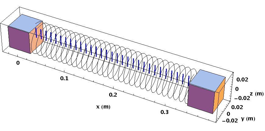
Figure 1.3: See figure 1.1 and 1.2. Projecting out the tetrad with space step $\lambda$.

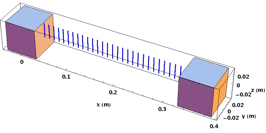
Figure 1.4: See figure 1.1 and 1.2 and 1.3. Ruler left by the projection.

1.2 Gauge fixing, the GW metric

If space-time is nearly flat, we can assume the metric to be written as

$$g_{\alpha\beta}=\eta_{\alpha\beta}+h_{\alpha\beta}\,,$$ (1.13)

where $\eta=\operatorname{diag}(-1,1,1,1)$ and $h$ is a perturbation such that $|h_{\alpha\beta}|\ll 1$. Notice component by component $\eta^{\alpha\beta}=\eta_{\alpha\beta}$ denotes the inverse.

We fix the global gauge by choosing harmonic gauge (see eq. (A.16)), so that:

$$h^{\alpha}_{\phantom{\alpha}\beta,\alpha}-\frac{1}{2}h^{\eta}_{\phantom{\eta}\eta,\beta}=0\,,$$ (1.14)

and name TT-gauge that specific local gauge-fixing of metric DOF such that:

$$\begin{split}h_{\mu 0}&=0\,,\\ \eta_{ij}h^{ij}=h_{i}^{i}&=0\,,\\ h_{ij;j}\simeq h_{ij,j}&=0\,,\end{split}$$ (1.15)

obviously the $h$ tensor retains only spatial components, it’s traceless and transverse (TT). We can always employ this choice, without loss of generality, since it won’t change the form of the physical observables made out of $R^{\mu}_{\phantom{\mu}\nu\sigma\eta}$.

We remind now that the connection for a nearly-linear theory is expressed by formula (A.4), and if the gauge choice is TT, most of the mixed components of $\Gamma^{\mu}_{\phantom{\mu}\alpha\beta}$ vanish or get simplified [20]:

$$\Gamma^{i}_{\phantom{i}00}=\Gamma^{0}_{\phantom{0}00}=\Gamma^{0}_{\phantom{0}0j} =0\,,$$ (1.16)

$$\Gamma^{0}_{\phantom{0}jk} =-\frac{1}{2}h_{jk,0}\,.$$ (1.17)

$$\Gamma^{i}_{\phantom{i}0j} =\frac{1}{2}h_{j\phantom{i},0}^{\phantom{j}i}\,.$$ (1.18)

only a few terms will survive due to the mentioned simplifications, to get from (1.6) (see appendix B):

$$\frac{\operatorname{d}^{2}x^{i}}{\operatorname{d}t^{2}}=\left(-2\Gamma^{i}_{\phantom{i}0j}-\Gamma^{i}_{\phantom{i}jk}v^{k}+\Gamma^{0}_{\phantom{i}jk}v^{i}v^{k}\right)v^{j}\,.$$ (1.19)

Thus in TT-gauge, in absence of external forces particles at rest ($v^{i}=0$) remain at rest forever, since they never accelerate. Hence their coordinates are good markers of position and time. We’ll never stress enough the point that we are now talking about coordinates; conversely distances are relative objects locally governed by geodesics acceleration equations, the presence of a tidal field may stretch or shrink them in this scenario according to (1.7).

Let’s summarise the ingredients we have collected so far:

1. we placed two bodies shielded from external disturbances in space and in free-fall (relative velocities are $\simeq 0$). Moreover this view of the coordinates is global and it’s just a choice, i.e. doesn’t modify physical observables, which are gauge-invariant functions of the Riemann tensor mapped by the laser phase [21].

2. We equipped space and time with rods and clocks independent on the presence of gravitational perturbations. Of course the situation will get more and more complicated the more curved space-time is: geodesics may cross and eclectic phenomena may appear. Nevertheless in the case of a small perturbation of the metric $h_{\mu\nu}$ we claim this to be suitable to our purposes.

3. If a gravitational radiative phenomenon occurs so to produce GW to travel till being plane in the premises of such a detection apparatus, tidal contributions to $h_{ij}$ will show up in adherence to Einstein’s theory. Hence variation of curvature will change the laser phase by changing its optical path.

If the perturbation were not there, the metric would be simply flat: $g_{\mu\nu}=\eta_{\mu\nu}$. With reference to the idle tetrad, the generator of infinitesimal motion along ${\boldsymbol{e}}_{1}$, mapped by the proper parameter $\sigma$ and by the laser beam, would get the following form:

$$\Omega^{\alpha\beta}=u_{\mu}\omega_{\nu}\epsilon^{\mu\nu\alpha\beta}\,,$$ (1.20)

since no acceleration is induced in that direction and we allow the moving tetrad to whirl with angular velocity $\omega$. The vector parameters are chosen such that:

$${\boldsymbol{u}}=\left[\begin{matrix}c\\ 0\\ 0\\ 0\end{matrix}\right]\,,\qquad{\boldsymbol{\omega}}=\xi\left[\begin{matrix}0\\ \nicefrac{{2\pi c}}{{\lambda}}\\ 0\\ 0\end{matrix}\right]\,,$$ (1.21)

indeed: ${\boldsymbol{u}}\parallel{\boldsymbol{e}}_{0}$ and ${\boldsymbol{\omega}}\parallel{\boldsymbol{e}}_{1}$. We can then normalise ${\boldsymbol{u}}$ so that ${\boldsymbol{u}}={\boldsymbol{e}}_{0}$. $\xi$ is an infinitesimal parameter. The rotating tetrad picks then the form:

$${\boldsymbol{e}}_{0}=\left[\begin{matrix}1\\ 0\\ 0\\ 0\end{matrix}\right]\,,\quad{\boldsymbol{e}}_{1}=\left[\begin{matrix}0\\ 1\\ 0\\ 0\end{matrix}\right]\,,\quad{\boldsymbol{e}}_{2}=\left[\begin{matrix}0\\ 0\\ \cos\omega t\\ \sin\omega t\end{matrix}\right]\,,\quad{\boldsymbol{e}}_{3}=\left[\begin{matrix}0\\ 0\\ -\sin\omega t\\ \cos\omega t\end{matrix}\right]\,,$$ (1.22)

where vectors have been properly normalised. Application of the $\Omega$ operator to the vectors give the infinitesimal variation of the vectors themselves:

$$\nabla_{{\boldsymbol{u}}}{\boldsymbol{e}}_{0} =\nabla_{{\boldsymbol{u}}}{\boldsymbol{u}}={\boldsymbol{0}}\,,$$ (1.23)

$$\nabla_{{\boldsymbol{u}}}{\boldsymbol{e}}_{1} ={\boldsymbol{0}}\,,$$ (1.24)

$$\nabla_{{\boldsymbol{u}}}{\boldsymbol{e}}_{2} =\xi\frac{2\pi c}{\lambda}{\boldsymbol{e}}_{3}\,,$$ (1.25)

$$\nabla_{{\boldsymbol{u}}}{\boldsymbol{e}}_{3} =-\xi\frac{2\pi c}{\lambda}{\boldsymbol{e}}_{2}\,,$$ (1.26)

as expected $\nabla_{{\boldsymbol{u}}}$ acts as an infinitesimal transporter of the tetrad along ${\boldsymbol{u}}$; moreover, its exponentiation will give the result for a finite parameter $\xi$. Let’s compute it for the evolution of ${\boldsymbol{e}}_{2}$:

$$\begin{split}\left(\exp\nabla_{{\boldsymbol{u}}}\right){\boldsymbol{e}}_{2}&=\sum_{j=0}^{\infty}\frac{1}{j!}\left(\nabla_{{\boldsymbol{u}}}\right)^{j}{\boldsymbol{e}}_{2}=\\ &=\sum_{j=0}^{\infty}\frac{1}{(2j)!}\left(\nabla_{{\boldsymbol{u}}}\right)^{2j}{\boldsymbol{e}}_{2}+\sum_{j=0}^{\infty}\frac{1}{(2j+1)!}\left(\nabla_{{\boldsymbol{u}}}\right)^{2j+1}{\boldsymbol{e}}_{2}\,,\end{split}$$ (1.27)

we now employ the facts:

$$\begin{split}\left(\nabla_{{\boldsymbol{u}}}\right)^{2}{\boldsymbol{e}}_{2}&=-\left(\frac{2\pi c}{\lambda}\xi\right)^{2}{\boldsymbol{e}}_{2}\,,\\ \left(\nabla_{{\boldsymbol{u}}}\right)^{2}{\boldsymbol{e}}_{3}&=\left(\nabla_{{\boldsymbol{u}}}\right)^{2}\nabla_{{\boldsymbol{u}}}{\boldsymbol{e}}_{2}=-\left(\frac{2\pi c}{\lambda}\xi\right)^{2}{\boldsymbol{e}}_{3}\,,\end{split}$$ (1.28)

to get

$$\left(\exp\nabla_{{\boldsymbol{u}}}\right){\boldsymbol{e}}_{2}={\boldsymbol{e}}_{2}\sum_{j=0}^{\infty}\frac{(-1)^{j}}{(2j)!}\left(\frac{2\pi c}{\lambda}\xi\right)^{2j}+{\boldsymbol{e}}_{3}\sum_{j=0}^{\infty}\frac{(-1)^{j}}{(2j+1)!}\left(\frac{2\pi c}{\lambda}\xi\right)^{2j+1}\,.$$ (1.29)

Finally, according to Taylor’s theorem and the series for sine and cosine, we get:

$${\boldsymbol{e}}_{2}^{\prime}=\left(\exp\nabla_{{\boldsymbol{u}}}\right){\boldsymbol{e}}_{2}=\cos\left(\frac{2\pi c}{\lambda}\xi\right){\boldsymbol{e}}_{2}+\sin\left(\frac{2\pi c}{\lambda}\xi\right){\boldsymbol{e}}_{3}\,,$$ (1.30)

therefore, if $\xi$ is an integer multiple of the ratio $\nicefrac{{\lambda}}{{c}}$, we get that the rotating tetrad is coincident with the reference idle one by imposing ${\boldsymbol{e}}_{2}^{\prime}={\boldsymbol{e}}_{2}$. Hence we can build a set of fiduciary points marking a ruler with pace $\lambda$, as planned.

Suppose a GW would come along direction ${\boldsymbol{e}}_{3}$, with reference to the idle tetrad placed along the first mirror surface. In TT-gauge, its relevant DOF can be expressed by means of two amplitudes $h_{\times}$ and $h_{+}$, properly added to the unperturbed flat-metric, to build an overall tensor as:

$$g_{\mu\nu}=\eta_{\mu\nu}+\left(\delta_{\mu 1}\delta_{\nu 1}-\delta_{\mu 2}\delta_{\nu 2}\right)h_{+}+\left(\delta_{\mu 2}\delta_{\nu 1}+\delta_{\mu 1}\delta_{\nu 2}\right)h_{\times}\,,$$ (1.31)

We remind that the gravity perturbation would act on the tetrad system as follows:

$$\begin{split}\Omega^{\mu\nu}{\boldsymbol{e}}_{\nu}&=\Omega^{\mu\nu}g_{\nu\chi}{\boldsymbol{e}}^{\chi}=\\ &=\Omega^{\mu\nu}\eta_{\nu\chi}{\boldsymbol{e}}^{\chi}+\Omega^{\mu\nu}h_{\nu\chi}{\boldsymbol{e}}^{\chi}\,,\end{split}$$ (1.32)

in fact, when crossing the space-time area deformed by the presence of a GW, a correction is added to the standard transporter, in the form of a Lorentz-rotational operator. In TT-gauge, by contracting the vectors ${\boldsymbol{e}}_{2}$ and ${\boldsymbol{e}}_{3}$ with the new transporter expression we’d get the eigenvalues equations:

$$\begin{split}\left(\nabla_{{\boldsymbol{u}}}\right)^{2}{\boldsymbol{e}}_{2}&=-\left(\frac{2\pi c}{\lambda}\right)^{2}\left(1-h_{\times}\right){\boldsymbol{e}}_{2}\,,\\ \left(\nabla_{{\boldsymbol{u}}}\right)^{2}{\boldsymbol{e}}_{3}&=-\left(\frac{2\pi c}{\lambda}\right)^{2}\left(1-h_{\times}\right){\boldsymbol{e}}_{3}\,,\end{split}$$ (1.33)

then, the net effect on the rotating tetrad for a finite elongation can be recovered by exponentiation; no computation needed, provided we make the parameter shift:

$$\xi\to\xi\sqrt{1-h_{\times}}\,,$$ (1.34)

to get:

$${\boldsymbol{e}}_{2}^{\prime}=\left(\exp\nabla_{{\boldsymbol{u}}}\right){\boldsymbol{e}}_{2}=\cos\left(\frac{2\pi c}{\lambda}\sqrt{1-h_{\times}}\xi\right){\boldsymbol{e}}_{2}+\sin\left(\frac{2\pi c}{\lambda}\sqrt{1-h_{\times}}\xi\right){\boldsymbol{e}}_{3}\,.$$ (1.35)

Since $h_{\times}$ is small we get:

$$\begin{split}{\boldsymbol{e}}_{2}^{\prime}=&\left(\cos\left(\frac{2\pi c}{\lambda}\xi\right)+h_{\times}\frac{\pi c}{\lambda}\xi\sin\left(\frac{2\pi c}{\lambda}\xi\right)\right){\boldsymbol{e}}_{2}+\\ &+\left(\sin\left(\frac{2\pi c}{\lambda}\xi\right)-h_{\times}\frac{\pi c}{\lambda}\xi\cos\left(\frac{2\pi c}{\lambda}\xi\right)\right){\boldsymbol{e}}_{3}\,,\end{split}$$ (1.36)

assume then for simplicity a multiple integer value $k$ of $\nicefrac{{\lambda}}{{c}}$ for the parameter $\xi$; we’ll then get:

$${\boldsymbol{e}}_{2}^{\prime}={\boldsymbol{e}}_{2}-h_{\times}k\pi{\boldsymbol{e}}_{3}\,,$$ (1.37)

and the final effect over $k$ wavelengths amounts on summing the space-time strain $h_{\times}$ acting as a phase shift over the tetrad. Notice this extra phase is what we can really measure by laser interferometry, and since $k=\left[\nicefrac{{L}}{{\lambda}}\right]$ - where $L$ now represents the flat-space distance between the mirrors and the square brackets designate integer part - it is straightforward to see that the longer the detection arm, the highest the precision in measuring the strain.

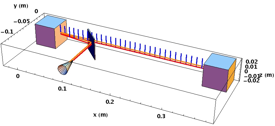
Figure 1.5: Interferometric measure of distance.

1.3 Spurious effects

A tetrad attached to the photons in the light beam will be rigidly tied to the reference mirror surface along ${\boldsymbol{e}}_{1}$. In spite of any shielding we may put around the mirror, residual stray forces as well as electromagnetic couplings may still be there, though reduced: the effect would be to add an effective acceleration to the mirror, inducing an extra phase-shift to the laser-beam. In formulae, a spurious Fermi-Walker transporter gets added to the original one:

$$\Omega^{\alpha\beta}=\tilde{a}^{\alpha}u^{\beta}-\tilde{a}^{\beta}u^{\alpha}\,,$$ (1.38)

where the $4$-acceleration $\tilde{{\boldsymbol{a}}}$ may be taken in the form:

$$\frac{e}{m}F^{\mu}_{\phantom{\mu}\chi}u^{\chi}+\frac{1}{m}f^{\mu}\,,$$ (1.39)

thus embedding EM forces and couplings in the Faraday stress-tensor $F^{\mu\nu}$ and stray, residual couplings into $f^{\mu}$. These last can of course be of any origin, from mechanical to static gravitational, to gradients of temperatures.

It is not customary to consider the problem on such a perspective. More often one solves the Einstein equations for a given energy-momentum distribution, deduces the form of the $g^{\mu\nu}$ metric and the related connection $\Gamma^{\mu}_{\phantom{\mu}\nu\sigma}$ and then calls “geodesics” the solution to the null geodesic equation in the given metric. If the “extra” accelerations are small as perturbations, the two ways are equivalent. We can still call geodesics those curves described in proper time by bodies in free fall in the globally unperturbed metric, and study the sources of acceleration noise causing the oscillations around these “ground state” geodesics.

To build up the EM spurious acceleration term, a Faraday stress tensor term must be coupled with a time-like vector representing a velocity. This last can be thought as composed by a drifting one, having a specific static orientation and a random one, highly variable in orientation: they both couple to high-frequency and low-frequency parts of $F^{\mu\nu}$. The new geodesics oscillate around the unperturbed ones; the effect on the spatial components can be upper limited by the norm of the random perturbation on a small time-scale (rapid oscillations) so that we can encompass it in a “circle” at fixed proper time. Along the curve on the proper time parameter the geodesic perturbation is thus embedded in a tube. For reference, see figure (1.6).

The nature of the spurious acceleration needs to be discussed more thoroughly:

1. it’s strongly space-dependent and localised: both the static and dynamic components depend on EM charge and currents distributions surrounding of the mirrors and sourcing electric and magnetic fields, and even for external causes (say, for instance the interplanetary magnetic field) the effect is rendered local by parasitic currents induced in conductors or in the mirrors themselves. Local charges, of static (DC) electric nature and parasitic currents will dominate the scene, justifying a low-velocity approximation in the estimate and a predominance of space derivatives and related momenta over the time ones:

   $$\left|\partial_{x}\right|\gg\left|\partial_{t}\right|\,.$$ (1.40)

2. The static contribution of EM and mechanical nature is highly predominant, thus the “drift” problem cannot be ignored. Therefore the concept of free-fall is not suitable to build an experiment under these circumstances: it is rather preferable to guarantee local motion to be almost-inertial, actively compensating for any drifting term by controlling the motion of the (first) reference mirror, “suspending” it to reduce the parasitic spring coupling to the shield too. Inertiality of this “spacecraft” can be naturally provided by going to outer space and exploiting the Keplerian gravitation around the Sun in the Solar System: motion is in fact inertial in the $5$ Lagrangian points of the Earth-Sun gravitational potential. Obviously for the noise and drag issue dedicated tactics must be planned and the device purposefully studied.

3. Dynamic contributions are faster Fourier components on the background of the static ones: basically magnetic or electric transients in nature, can be nevertheless thought to be suppressed by the $\nicefrac{{e}}{{m}}$ dependence. The larger and more sophisticated the conductors, the more unpredictable the correlated effect could be; we’ll have more space to discuss these effects in the noise chapter and we’ll retain only first-order components in the velocities here.

Our conclusion on the spurious acceleration is the following:

• it may be thought as an additional acceleration operator, whose effect is adding an undesired spatial offset, variable with time, to the positions of the mirrors. In other words, curvature picks up a locally generated term originated by many sources mainly of EM and static gravitational nature. The detection of tidal effects by perturbed freely-falling mirrors is thus jeopardised by an extra phase, variable with time, picked up by the laser on its travel and due to the real, gauge-invariant change in position of the mirrors: we will describe it as an effect in the mirrors velocities;

• according to Mach’s principle it is impossible to distinguish the local from the non-local source since tidal effects sum linearly; nevertheless EM fields are gauge invariant objects, therefore observable and measurable: this is valid for fields generated by local distributions of charges and currents but also for external ones. The same occurs for local gravitational contributions, which can be very well approximated up to quadrupole expansions. In summary this part can be detected and “projected” out of the noise picture.

• Limiting the jitter and compensating for the drift are the only feasible methods to mimic a condition of motion similar to theoretical free-fall. We call the first strategy “noise reduction” and the second “drag-free”.

Figure 1.6: Geodesics of freely falling mirrors in space-time. Simplified picture in $3$ dimensions; geodesics are traced in space-time as curves (green) parametrised along the up-down direction on proper time. A laser beam shone from the first bounces on the second and then back. Left: unperturbed geodesics in absence of any residual acceleration. Right: noisy geodesics embedded into maximal space-like circles whose norm is the perturbation scale; as function of the proper time the embedding takes the shape of a tube per each mirror.

In the low velocity approximation the perturbed geodesic acceleration equation becomes (see appendix for a proof, eq. (B.19)):

$$\frac{\operatorname{d}^{2}x^{i}}{\operatorname{d}t^{2}}=\left(-\Gamma^{i}_{\phantom{i}00}-2\Gamma^{i}_{\phantom{i}0j}v^{j}+\Gamma^{0}_{\phantom{0}00}v^{i}\right)+e\left(F^{i}_{\phantom{i}0}+F^{i}_{\phantom{i}k}v^{k}\right)+\left(f^{i}-f^{0}v^{i}\right)\,.$$ (1.41)

and if the gauge choice is TT,

$$\begin{split}\frac{\operatorname{d}^{2}x^{i}}{\operatorname{d}t^{2}}=\frac{\operatorname{d}v^{i}}{\operatorname{d}t}&=a^{i}-2\Gamma^{i}_{\phantom{i}0j}v^{j}+\frac{e}{m}\left(F^{i}_{\phantom{i}0}+F^{i}_{\phantom{i}k}v^{k}\right)+\left(f^{i}-f^{0}v^{i}\right)=\\ &=a^{i}-2\Gamma^{i}_{\phantom{i}0j}v^{j}+\frac{e}{m}\left(E^{i}+\epsilon^{ijk}v_{j}B_{k}\right)+\left(f^{i}-f^{0}v^{i}\right)\,,\end{split}$$ (1.42)

where we expanded the expression of the Faraday tensor and introduced the electric ${\boldsymbol{E}}$ and magnetic ${\boldsymbol{B}}$ fields. The term obviously hides all the geometric peculiarities of the machinery around the mirror, but we can deal with the whole of it later, in the noise section. Notice this set of terms embodies our former choices: they are strongly distributional-dependent, slowly varying, locally sourced.

We can now introduce the definition of correlator:

$$C_{\Delta\theta}(\tau)=\int_{-\infty}^{\infty}\Delta\theta(t)\Delta\theta(\tau-t)\operatorname{d}t\,,$$ (1.43)

so that the squared Power Spectral Density (PSD) associated with the phase correlator is the Fourier transform of the last expression:

$$S_{\Delta\theta}(\omega)=\int_{-\infty}^{\infty}e^{-\imath\omega\tau}C_{\Delta\theta}(\tau)\operatorname{d}\tau\,.$$ (1.44)

Hence, (1.42) may be rearranged and converted to squared PSD, assuming the terms are all uncorrelated as:

$$S_{a}\simeq\omega^{2}S_{v}+S_{\text{GW, tidal}}+S_{\text{EM, noise}}+S_{\text{extra, noise}}\,,$$ (1.45)

as it can be seen, several competitors concur to the residual acceleration PSD in the former equation.

1.4 Detection

According to formula (1.35) and by simple geometric arguments, the cosine of the angle $\theta(\xi)$ instantaneously spanned between ${\boldsymbol{e}}_{2}$ and ${\boldsymbol{e}}_{2}^{\prime}$ is:

$$\cos\theta\left(\xi\right)={\boldsymbol{e}}_{2}^{\prime}\cdot{\boldsymbol{e}}_{2}=\cos\left(\frac{2\pi c}{\lambda}\sqrt{1-h_{\times}}\xi\right)\,,$$ (1.46)

so that, now replacing $h_{\times}$ with a generic wave-strain $h$:

$$\theta\left(\xi\right)=\frac{2\pi c}{\lambda}\sqrt{1-h}\xi=\frac{2\pi c\xi}{\lambda}-\frac{\pi c\xi}{\lambda}h+O\left(h^{2}\right)\,$$ (1.47)

by dimensional power counting, we deduce now that $\xi$ must be a time, in fact, since $h$ is dimensionless and the argument of transcendental functions have to be dimensionless too, we have $\left[\xi\right]\sim\left[\nicefrac{{\lambda}}{{c}}\right]=\left[\text{time}\right]$ and identify $\xi\equiv t$. Moreover, we may very well think $h$ to be small, but we need to consider arbitrary lengths of the laser beam path, or conversely arbitrary frequency span of the GW perturbation, at least in principle. We may think of $h=h(t)=h_{0}\cos\omega_{\text{GW}}t$, where $h_{0}$ can be thought as a slowly varying function of time so to be considered almost constant over a large multiple of $\lambda_{\text{GW}}$. In this sort of rapidly rotating wave approximation we get:

$$\theta\left(t\right)\simeq\frac{2\pi c}{\lambda}t-\frac{\pi c}{\lambda}th_{0}\left(t\right)\cos\left(\omega_{\text{GW}}t\right)\,$$ (1.48)

by time derivative we get to order $h$:

$$\begin{split}\frac{\operatorname{d}\theta(t)}{\operatorname{d}t}=&-\frac{\pi c}{\lambda}h_{0}(t)\cos\left(\omega_{\text{GW}}t\right)+\frac{\pi c}{\lambda}\omega_{\text{GW}}t\,h_{0}(t)\sin\left(\omega_{\text{GW}}t\right)+\\ &-\frac{\pi c}{\lambda}t\,h_{0}^{\prime}(t)\cos\left(\omega_{\text{GW}}t\right)+\frac{2\pi c}{\lambda}\,.\end{split}$$ (1.49)

We now wish to evaluate this last across one full reflection period between the mirrors, i.e. from $t=\tau$, till $t=\tau+\Delta T_{\text{flight}}$ and this latter to $t=\tau+2\Delta T_{\text{flight}}$, where $\Delta T_{\text{flight}}=\nicefrac{{L}}{{c}}$ is the laser flight time between unperturbed mirrors in flat curvature. We get:

$$\begin{split}\frac{\operatorname{d}\theta}{\operatorname{d}t}&\Bigr{|}_{\tau-\frac{L}{c}}-\frac{\operatorname{d}\theta}{\operatorname{d}t}\Bigr{|}_{\tau}+\frac{\operatorname{d}\theta}{\operatorname{d}t}\Bigr{|}_{\tau-2\frac{L}{c}}-\frac{\operatorname{d}\theta}{\operatorname{d}t}\Bigr{|}_{\tau-\frac{L}{c}}=\\ =&\frac{\pi c}{\lambda}\Bigl{(}h_{0}(\tau)\cos\left(\omega_{\text{GW}}\tau\right)-\tau\omega_{\text{GW}}h_{0}(\tau)\sin\left(\omega_{\text{GW}}\tau\right)+\\ &-h_{0}\left(\tau-\frac{2L}{c}\right)\cos\left(\omega_{\text{GW}}\left(\tau-\frac{2L}{c}\right)\right)+\\ &+\left(\tau-\frac{2L}{c}\right)\omega_{\text{GW}}h_{0}\left(\tau-\frac{2L}{c}\right)\sin\left(\left(\tau-\frac{2L}{c}\right)\omega_{\text{GW}}\right)\Bigr{)}\,,\end{split}$$ (1.50)

where we took $h_{0}^{\prime}(t)\simeq 0$. Finally, in the low frequency GW approximation, we get, back from $\tau$ to $t$:

$$\frac{\operatorname{d}\Delta\theta(t)}{\operatorname{d}t}=\frac{\pi c}{\lambda}\left(h(t)-h\left(t-\frac{2L}{c}\right)\right)+O\left(\omega_{\text{GW}}^{2}\right)\,.$$ (1.51)

For low-frequency almost-plane GWs a laser beam shone between two mirrors in drag-free motion with respect to each-other suffers a phase shift whose instantaneous time derivative depends only on the wave strain evaluated at the laser shining point. If we now name $\omega_{0}=\nicefrac{{2\pi c}}{{\lambda}}$, the former equation shows that the relative variation of pulsation is only a function of the causal strain difference [10]:

$$\frac{\Delta\omega(t)}{\omega_{0}}\simeq\frac{1}{2}\left(h(t)-h\left(t-\frac{2L}{c}\right)\right)\,.$$ (1.52)

In fact, such an estimate is true for any polarisation of the incoming GW. To display the formula in its full glory we may define an angle $\phi$ span on the common plane by the laser beam and the “Poynting” vector of the GW, to write:

$$\begin{split}\frac{\Delta\omega(t)}{\omega_{0}}\simeq&\frac{1}{2}\left(h_{+}(t)-h_{+}\left(t-\frac{2L}{c}\right)\right)\cos 2\phi+\\ &+\frac{1}{2}\left(h_{\times}(t)-h_{\times}\left(t-\frac{2L}{c}\right)\right)\sin 2\phi\,,\end{split}$$ (1.53)

which reduces to (1.52) for optimal orientation of the detector, $\phi=0$.

1.5 Noise

As mentioned by means of general arguments, if the two mirrors are in motion, i.e. their velocity is not null with respect to one another, then there’s a real shift in position and hence in mutual distance with respect to the perfect TT frame. Obviously the accuracy of the TT-gauge definition in itself is not affected by such a motion, but the arising acceleration competes with the curvature induced by the GW perturbation $h$ and focused in eq. (1.51). In other words, if we’d like to depict the scene on the pure accounts of coordinates, detected by some sophisticated readout device as our laser (or an electrostatic capacitance detector), the shift in phase can be easily evaluated from the shift in position:

$$\begin{split}\Delta\theta(t)=\frac{2\pi}{\lambda}\Bigl{(}&x_{1}(t)-x_{2}\left(t-\frac{L}{c}\right)+\\ +&x_{1}\left(t-\frac{2L}{c}\right)-x_{2}\left(t-\frac{L}{c}\right)\Bigr{)}\,,\end{split}$$ (1.54)

where $x_{1}(t)$ is the coordinate of the mirror sending and collecting the laser beam, while $x_{2}(t)$ is that of the reflecting one. The shift is calculated to first order in $\nicefrac{{v}}{{c}}$, and if the frequency of measurement is $\ll\nicefrac{{c}}{{L}}$ we may approximate (1.54) to

$$\Delta\theta(t)=\frac{4\pi}{\lambda}\Delta L(t)\,.$$ (1.55)

where $\Delta L(t)=x_{1}(t)-x_{2}(t)$.

The former argument is somehow of questionable value when crossed with the TT-gauge demands. It is not easy to deal with observables and measurability in GR, but one sure thing is that distance is not an observable quantity. That’s why we’ve been spending so much time in building a distance estimator not relying on any absolute distance, but the fixed velocity scale $c$. Conversely the laser phase shift or better its pulsation shift is a directly measurable object, and a causal carrier of the effect of a gravitational distortion in space-time. We’d prefer to convert the former argument into one on velocities and phases: according to the geodesic equation in TT-gauge if bodies are idle to start with, they pick up no further acceleration in time; estimates on velocities and pulsations are more reliable and in the correct spirit though. The equivalent of (1.54) is thus:

$$\frac{\Delta\omega(t)}{\omega_{0}}=\frac{1}{c}\Bigl{(}v_{1}(t)-2v_{2}\left(t-\frac{L}{c}\right)+v_{1}\left(t-\frac{2L}{c}\right)\Bigr{)}\,,$$ (1.56)

and to very low frequency with respect to $\nicefrac{{c}}{{L}}$ we get:

$$\frac{\Delta\omega(t)}{\omega_{0}}\simeq\frac{2\Delta v(t)}{c}\,.$$ (1.57)

where now $\Delta v(t)\doteq v_{1}(t)-v_{2}(t)$.

In order to open a detailed discussion on noise, correlators and PSDs of the phase shift must be built in time. Similar quantities can be built for each velocity signal $v_{i}(t),\,i=1,2$ and for the instantaneous velocity difference $\Delta v(t)$: $S_{\Delta v}(\omega)$, $S_{v_{i}}(\omega),\,i=1,2$, are the PSD of the sub-indicated quantities at the frequency $\omega$. We are implicitly assuming velocities to be joint stationary random processes, so that from the Doppler shift in equation (1.56) we deduce a squared PSD due to non-tidal (non-GW) motion with the following form:

$$\begin{split}S_{\nicefrac{{\Delta\omega}}{{\omega_{0}}}}(\omega)=&\frac{4S_{\Delta v}(\omega)}{c^{2}}\cos\left(\frac{\omega L}{c}\right)+\\ &+8\sin^{2}\left(\frac{\omega L}{2c}\right)\left(\frac{S_{v_{2}}(\omega)}{c^{2}}-\cos\left(\frac{\omega L}{c}\right)\frac{S_{v_{1}}(\omega)}{c^{2}}\right)=\\ \simeq&\frac{4S_{\Delta v}(\omega)}{c^{2}}\,,\end{split}$$ (1.58)

and the last approximation holds for $\nicefrac{{\omega L}}{{c}}\ll 1$.

Summarising the difference of forces acting on the mirrors as $\Delta F=F\left({\boldsymbol{x}}_{2}\right)-F\left({\boldsymbol{x}}_{1}\right)$, according to the geodesic deviation equations (B.39) or (B.41) to order $h$ and up to order $v$ in the velocities we’d get:

$$m\frac{\operatorname{d}v^{i}(t)}{\operatorname{d}t}\simeq-m\dot{h}_{j}^{\phantom{j}i}v^{j}(t)+\Delta F(t)\,,$$ (1.59)

assume then the usual form for an incoming GW: $h(t)=h_{0}\cos\omega_{\text{GW}}t$, where $h_{0}$ is a profile function so slowly varying with time we can consider it almost constant, very small in amplitude. The Fourier-space implicit propagator obtained from eq. (1.59) looks like:

$$\frac{\Delta F(\omega)}{m}=\frac{1}{2}\imath\left(-2\omega v(\omega)-h_{0}\omega_{\text{GW}}v\left(\omega-\omega_{\text{GW}}\right)+h_{0}\omega_{\text{GW}}v\left(\omega+\omega_{\text{GW}}\right)\right)$$ (1.60)

and in the limit of small $h_{0}$ amplitude we get for the square modulus of the velocity in Fourier space:

$$\left|v(\omega)\right|^{2}=\frac{\Delta F^{2}(\omega)}{m^{2}\omega^{2}}+O\left(h_{0}\right)\,,$$ (1.61)

thus resulting in a velocity squared PSD:

$$S_{v}(\omega)\simeq\frac{S_{\Delta F}(\omega)}{m^{2}\omega^{2}}\,.$$ (1.62)

Employing the relation between velocity and variation of pulsation in Fourier domain, eq. (1.58), we can deduce the conversion relation between force PSD and laser pulsation variation PSD:

$$S_{\nicefrac{{\Delta\omega}}{{\omega_{0}}}}\simeq\frac{4S_{\Delta v}(\omega)}{c^{2}}=\frac{4}{c^{2}}\frac{S_{\nicefrac{{\Delta F}}{{m}}}(\omega)}{\omega^{2}}\,,$$ (1.63)

thus any difference of force acting on the mirrors would induce a phase variation in the laser according to the latter expression. Notice the effect is suppressed by a factor $\nicefrac{{1}}{{\omega^{2}}}$. We conclude that a TT-gauged frame can be built in space-time by means of drag-free mirrors, provided external forces in difference are suppressed in the measurement bandwidth to the point of being considered negligible. The real observable in this scenario is the laser phase; apart from passing-by considerations, we never introduced or relied in absolute space or distances with the exception of the laser wavelength, a space elongation marked in fact by a phase.

One final remark here concerns the real definition of a length and time standard on-board a space mission. These are available from the interferometer and the time stamp of the data.

Again, the key feature for absolute calibration of the difference of displacement signal is the conversion relation between laser phase and equivalent displacement by

$${\Delta}x=\frac{{\Delta}\phi}{2\pi}\lambda\,,$$ (1.64)

where $\lambda$ is the laser wavelength. The absolute distance calibration is then limited by the combined accuracy of the knowledge of $\lambda$ and that of the conversion of the phase meter signal into radians or cycles, the latter being evaluated to $\nicefrac{{50}}{{10^{6}}}$ accuracy.

The scale factor of the time tagging of data is the other intervening factor. Noticeably what matters is the absolute accuracy on time intervals and not the definition of an absolute universal time. On purpose the LTP experiment will carry clocks on-board with accuracy $\sigma_{\nicefrac{{{\Delta}t}}{{t}}}\simeq 10^{-6}$, which will provide a definition of experimental time beats and a time length comparable to the intrinsic laser $\nicefrac{{1}}{{\nu}}=\nicefrac{{\lambda}}{{c}}$.

1.6 Laser interferometers and phase shift

The suppression of forces $\Delta F$ with PSD $S_{\Delta F}$ with non-gravitational origin, local or non-local be their nature, is mandatory in the measurement bandwidth to ensure the dominance of GW spectrum. We may now clear the smoke and start calling the mirrors and their envelope as LISA or LTP, since these missions will be embodying the abstract concepts we put at play so far. It’s impossible to annihilate every disturbance aboard the LISA space-crafts and hence a requirement over forces PSD has been cast, demanding:

$$S^{\nicefrac{{1}}{{2}}}_{\nicefrac{{\Delta F}}{{m}},\,\text{LISA}}(\omega)\leq\sqrt{2}\times 3\times 10^{-15}\,\nicefrac{\mathrm{m}}{\mathrm{s^{2}\sqrt{Hz}}}\,,$$ (1.65)

for a frequency $f>0.1\,\mathrm{mHz}$. This corresponds to a relative pulsation shift PSD in adherence to (1.63) like:

$$S^{\nicefrac{{1}}{{2}}}_{\nicefrac{{\Delta\omega}}{{\omega_{0}}},\,\text{LISA}}=\frac{c\omega}{2}S^{\nicefrac{{1}}{{2}}}_{\nicefrac{{\Delta F}}{{m}},\,\text{LISA}}(\omega)\simeq\frac{2.83\times 10^{-23}}{\omega\,\nicefrac{{1}}{{Hz}}}\,\nicefrac{\mathrm{1}}{\mathrm{\sqrt{Hz}}}\,.$$ (1.66)

The interferometer itself provides some measurement noise, expressed as an equivalent optical path fluctuation ${\delta}x$ for each passage of the light through the interferometer arm. A single arm interferometer hence suffers a relative pulsation shift per pass:

$$\frac{\Delta\omega(t)}{\omega_{0}}\simeq\frac{1}{c}\frac{\operatorname{d}{\delta}x(t)}{\operatorname{d}t}=\frac{\omega}{c}{\delta}x(t)\,,$$ (1.67)

so that, back and forth the added equivalent PSD square of the noise will be

$$S_{\nicefrac{{\Delta\omega}}{{\omega_{0}}},\,\text{laser}}(\omega)\simeq 2\frac{\omega^{2}}{c^{2}}S_{{\delta}x}(\omega)\,,$$ (1.68)

or, in terms of accelerations, by virtue of (1.63):

$$S^{\nicefrac{{1}}{{2}}}_{\nicefrac{{\Delta F}}{{m}},\,\text{laser}}(\omega)\simeq\frac{\omega^{2}}{\sqrt{2}}S_{{\delta}x}^{\nicefrac{{1}}{{2}}}(\omega)\,.$$ (1.69)

The corresponding requirement for the interferometer is to achieve a path length noise of $S_{{\delta}x}^{\nicefrac{{1}}{{2}}}\leq 20\,\nicefrac{\mathrm{pm}}{\mathrm{\sqrt{Hz}}}$, so that finally from (1.68) or (1.69) we may deduce the following figures:

$$S^{\nicefrac{{1}}{{2}}}_{\nicefrac{{\Delta\omega}}{{\omega_{0}}},\,\text{laser}}(\omega) \simeq 9.43\times 10^{-20}\frac{\omega}{\mathrm{Hz}}\nicefrac{\mathrm{1}}{\mathrm{\sqrt{Hz}}}\,,$$ (1.70)

$$S^{\nicefrac{{1}}{{2}}}_{\nicefrac{{\Delta F}}{{m}},\,\text{laser}}(\omega) \simeq 1.41\times 10^{-11}\frac{\omega^{2}}{\mathrm{Hz}^{2}}\nicefrac{\mathrm{m}}{\mathrm{s^{2}\sqrt{Hz}}}\,.$$ (1.71)

The force noise in (1.65) and the interferometer one in (1.69) cross at $\omega\simeq 2\pi\times 2.75\,\mathrm{mHz}\sim 2\pi\times 3\,\mathrm{mHz}\doteq\omega_{c}$, thus allowing to relax the requirement in (1.65) to:

$$\begin{split}S^{\nicefrac{{1}}{{2}}}_{\nicefrac{{\Delta F}}{{m}},\,\text{LISA}}(\omega)&\to S^{\nicefrac{{1}}{{2}}}_{\nicefrac{{\Delta F}}{{m}},\,\text{LISA}}(\omega)\left(1+\left(\frac{\omega}{\omega_{c}}\right)^{4}\right)^{\nicefrac{{1}}{{2}}}=\\ &=\sqrt{2}\times 3\times 10^{-15}\left(1+\left(\frac{\omega}{2\pi\times 3\,\mathrm{mHz}}\right)^{4}\right)^{\nicefrac{{1}}{{2}}}\,\nicefrac{\mathrm{m}}{\mathrm{s^{2}\sqrt{Hz}}}\,.\end{split}$$ (1.72)

This last formula is in fact a minimal lower interpolation of (1.65) and (1.69). Graphs of these latter together with (1.72) and their $S_{\nicefrac{{\Delta\omega}}{{\omega_{0}}}}^{\nicefrac{{1}}{{2}}}$ equivalents as functions of frequency can be inspected in figure 1.7. In limiting cases we’d get from (1.72):

$$\begin{split}S^{\nicefrac{{1}}{{2}}}_{\nicefrac{{\Delta F}}{{m}},\,\text{LISA}}(\omega)\underset{\omega\ll 2\pi\times 3\,\mathrm{mHz}}{=}&4.24\times 10^{-15}\,\nicefrac{\mathrm{m}}{\mathrm{s^{2}\sqrt{Hz}}}+O\left(\omega^{2}\right)\\ S^{\nicefrac{{1}}{{2}}}_{\nicefrac{{\Delta F}}{{m}},\,\text{LISA}}(\omega)\underset{\omega\gg 2\pi\times 3\,\mathrm{mHz}}{=}&1.20\times 10^{-11}\left(\frac{\omega}{\mathrm{Hz}}\right)^{2}\,\nicefrac{\mathrm{m}}{\mathrm{s^{2}\sqrt{Hz}}}+O\left(\left(\frac{1}{\omega}\right)^{2}\right)\end{split}$$ (1.73)

This requirement needs to be qualified and it is not testable on ground [22, 23]. By virtue of (1.58) we deduce also that limiting the noise in speed difference only by limiting forces in difference may become inaccurate for frequencies larger than $3-4\,\mathrm{mHz}$. However, the assumptions to get to (1.58) are very reliable and if the fluctuations in velocity of the mirrors are independent, the “difference of forces” approach represents a worst-case occurrence. If the noise would be partly correlated, the dangerous part of it would still be the one mimicking residual differential acceleration.

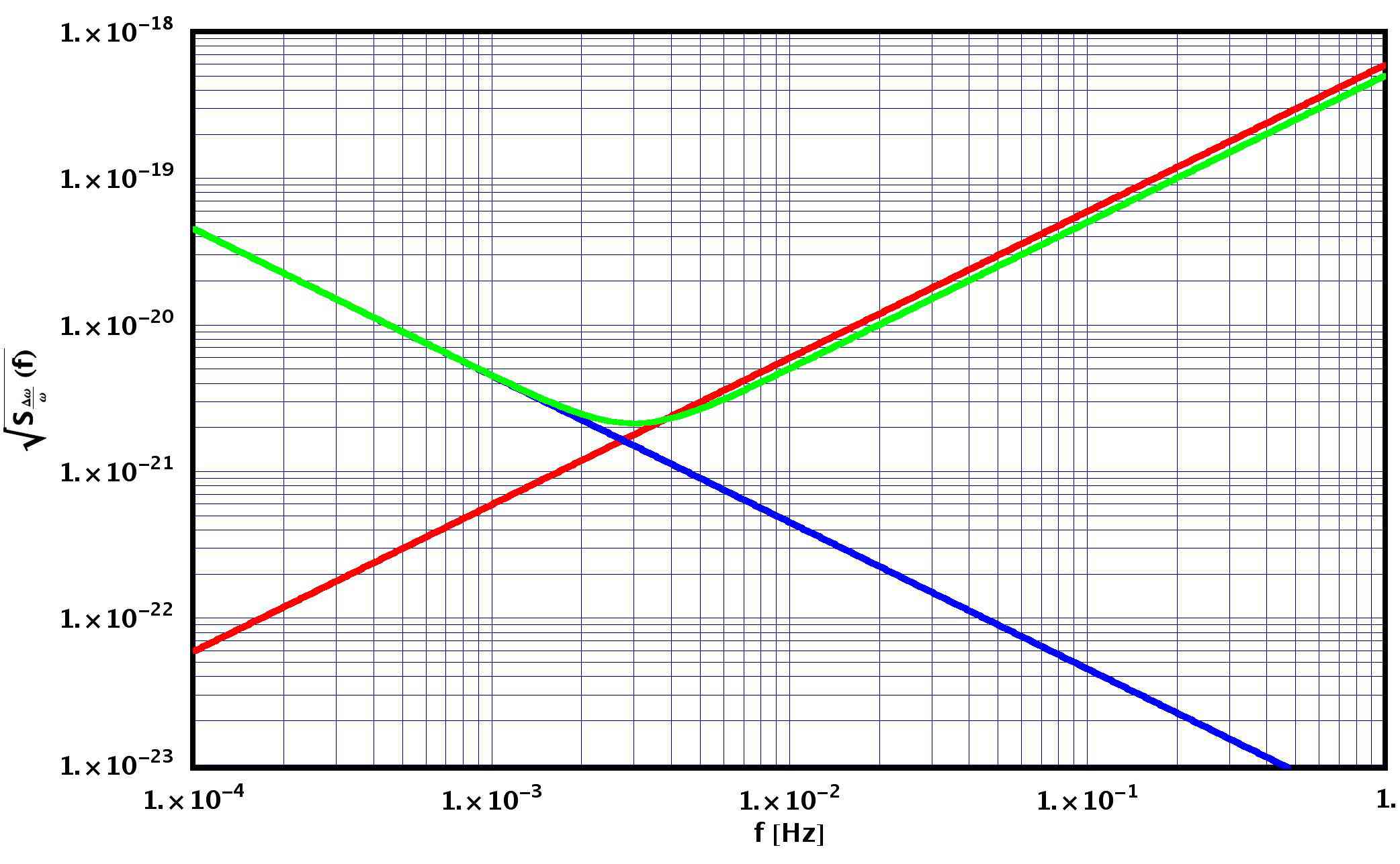
Figure 1.7: Upper: noise PSDs in $\nicefrac{{\Delta\omega}}{{\omega_{0}}}$ for forces difference (blue), interferometer (red) and relaxed noise requirement of forces difference (green). Green line represents LISA’s targeted sensitivity. Lower: noise PSDs in $\nicefrac{{\Delta F}}{{m}}$, same colour codes.

We’d like finally to give one more link between PSD and curvature as follows. The above discussion has been cast in terms of speed frames and frequency shifts; the requirements can nevertheless be restated in terms of components of the Riemann tensor only. Back to eq. (1.52), we can write

$$\frac{\Delta\omega(\omega)}{\omega_{0}}=\frac{1}{2}\left(1-e^{-\imath\frac{2L\omega}{c}}\right)h(\omega)\underset{\omega\ll\nicefrac{{c}}{{2L}}}{=}\imath\omega\frac{L}{c}h(\omega)+O\left(\omega^{2}\right)\,,$$ (1.74)

to find, by means of (1.63):

$$S^{\nicefrac{{1}}{{2}}}_{h}(\omega)\simeq\frac{2}{L\omega^{2}}S^{\nicefrac{{1}}{{2}}}_{\nicefrac{{\Delta F}}{{m}}}\,.$$ (1.75)

If we consider now the expression for the linearised Riemann tensor, we’d have:

$$R_{\mu\nu\rho\sigma}\simeq\frac{1}{2}\left(h_{\sigma\mu,\nu,\rho}-h_{\sigma\nu,\mu,\rho}+h_{\rho\nu,\mu,\sigma}-h_{\rho\mu,\nu,\sigma}\right)\,,$$ (1.76)

specialising to radiation and TT-gauge, the only survivors would be (see [16] or appendix A):

$$R_{0k0j}(t)=-\frac{1}{2}h_{kj,0,0}(t)\,,$$ (1.77)

therefore in Fourier space (we bring back the $c$ constant by dimensional arguments):

$$R_{0k0j}(\omega)=-\frac{\omega^{2}}{2c^{2}}h_{kj}(\omega)\,.$$ (1.78)

By joining (1.75) and (1.78) we can thus deduce that every differential force $\Delta F$ mimics a curvature noise with PSD:

$$S^{\nicefrac{{1}}{{2}}}_{R}(\omega)=\frac{\omega^{2}}{2c^{2}}S^{\nicefrac{{1}}{{2}}}_{h}(\omega)\simeq\frac{1}{c^{2}L}S^{\nicefrac{{1}}{{2}}}_{\nicefrac{{\Delta F}}{{m}}}(\omega)\,,$$ (1.79)

the pre-factor can be calculated in our conditions to give:

$$S^{\nicefrac{{1}}{{2}}}_{R}(\omega)\simeq 2.2\times 10^{-27}\,\mathrm{\frac{s^{2}}{m^{3}}}\times S^{\nicefrac{{1}}{{2}}}_{\nicefrac{{\Delta F}}{{m}}}(\omega)\,.$$ (1.80)

The requirement in (1.72) transforms into a curvature resolution of order $10^{-41}\,\nicefrac{\mathrm{1}}{\mathrm{m^{2}\,\sqrt{Hz}}}$, i.e. for a signal at $0.1\,\mathrm{mHz}$ integrated over a cycle, this gives a resolution of order $10^{-43}\,\nicefrac{\mathrm{1}}{\mathrm{m^{2}}}$, a figure which may be compared to the scale of the curvature scalar exerted by the Sun field at LISA location, about $10^{-30}\,\nicefrac{\mathrm{1}}{\mathrm{m^{2}}}$.

1.7 The Laser Interferometer Space Antenna

The Laser Interferometer Space Antenna (LISA) will be launched in 2017 by the combined efforts of the ESA and NASA. Nevertheless the concept of building off-ground interferometric detectors of GWs dates back to the 70’s; quite a variety of designs were advanced at the time [24].

More recently, laser technology allowed for designing very long baseline detectors, and ESA received plans for the Laser Antenna for Gravitational-radiation Observation in Space (LAGOS) project, which considered a constellation of three drag-free satellites orbiting around the Sun at $1\,\mathrm{AU}$. In fact this project looks quite similar to LISA, but the arm-lengths ranged $10^{6}\,\mathrm{km}$.

Seeking for alternative designs in order to validate the mission, ESA considered two parallel proposals: LISA and SAGITTARIUS, the former orbiting around the Sun, the latter around Earth, both extending the number of satellites to $6$. LISA was dropped at start, probably because of the complicated space-crafts setup, each of which hosting a test mirror, flying coupled in pairs, with a laser arm to control mutual motion, and the spare, long-baseline one to detect GW. Thanks to the effort of the “Team X” at Jet Propulsion Laboratory, conclusion was drawn that the constellation could be reduced to $3$ satellites each hosting $2$ mirrors. Eventually this simplification brought LISA back to the attention of the agency, where it was validated and chosen as effective mission.

LISA is then a constellation of $3$ space-crafts (SC) orbiting at $\nicefrac{{D}}{{2}}=1\,\mathrm{AU}$ from the sun, sharing Earth’s orbit with some $20$ degrees delay. The space-probes form an equilateral triangle and - as mentioned already - each of them hosts a couple of test-masses (TM) in free fall. An Electrode Housing (EH) and a set of capacitive Gravitational Reference Sensors (GRS) surround each TM and constitutes an Inertial Sensor (IS) capable of monitoring TM position and angular attitude. Each IS is coupled to a telescope and a laser and shares with the other on-board an interferometer Optical Bench (OB). A laser beam is shone from each satellite towards the independent far satellites, gets captured by the proper telescope there and sent back in “phase locking” after hitting the “alien” TMs. Figure 1.8 may help focusing the picture.

Each laser’s phase is locked either to its companion on the same SC, forming the equivalent of a beam-splitter, or to the incoming light from the distant SC, forming the equivalent of an amplifying mirror, or light transponder. The overall effect is that the three SC function as a Michelson interferometer with a redundant third arm. The arm-length size, ranging $5\times 10^{6}\,\mathrm{km}$, was chosen to optimise the sensitivity at the frequencies of known sources: increasing the arm-length improves sensitivity to low frequency GW strain (coming from massive black holes, for example).

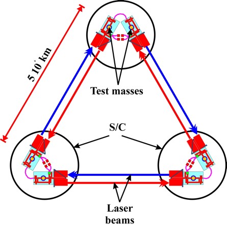
Figure 1.8: Closeup on LISA constellation and laser beams across the space-probes.

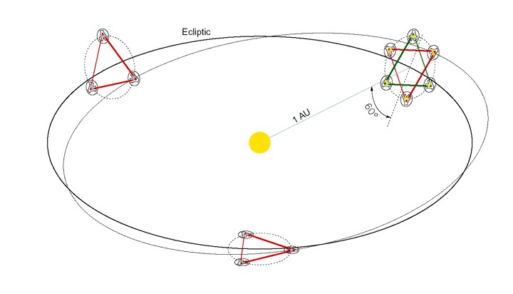
Figure 1.9: LISA’s orbit will be the same as Earth’s, following the planet by some $20$ degrees delay. The equilateral constellation will be rotating along its centre of mass while revolving around the Sun.

Each SC is meant as a protection against external disturbances for the TMs. Inside the SC, the ISs and relative TMs are obviously oriented with a mutual angle of $\nicefrac{{\pi}}{{3}}\,\mathrm{rad}$. This non-orthogonality of the reference allows for the so called “drag-free” control of SC (see figure 1.10): each SC is free to chase both the TMs motion along the bisector of the “sensing directions” (the laser beam ones) and can re-adjust the TMs positions by virtue of capacitance actuation voltages.

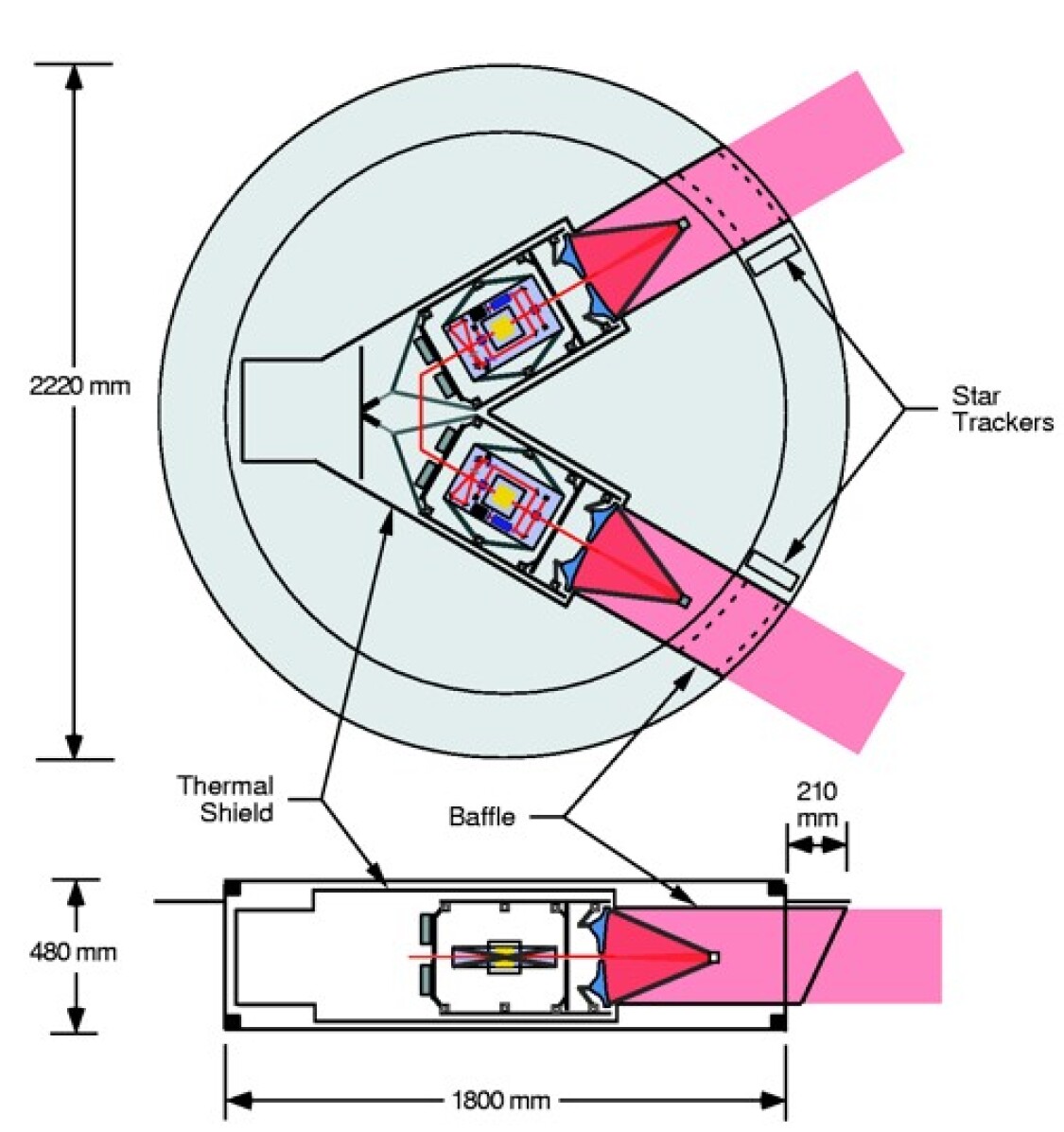
Figure 1.10: LISA’s SC internal structure. The so-called “Y”-shape is critical for accomplishing the mission demands. Top view shows the SC from top, details of the test-masses can be seen inside the telescopes. Bottom view shows the SC from the side.

(a)	(b)
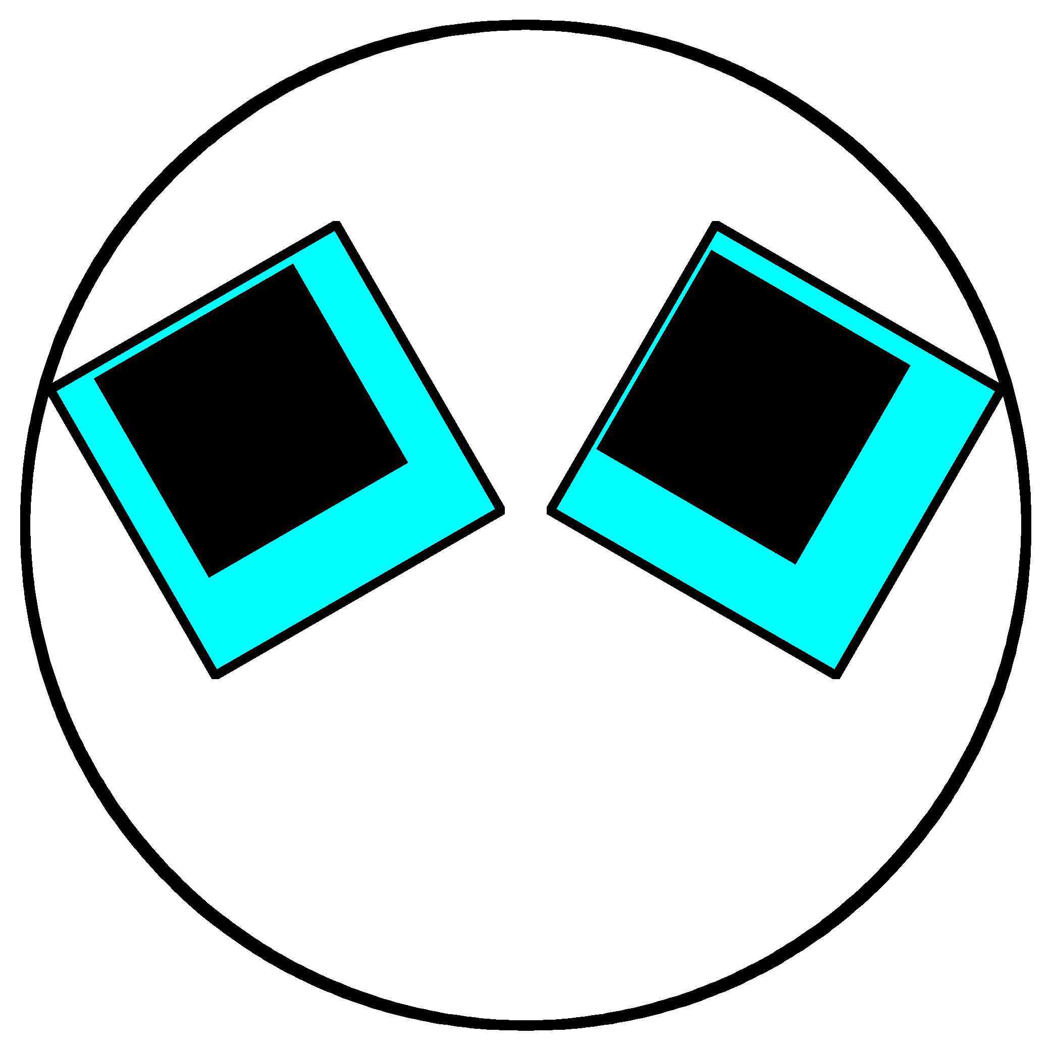
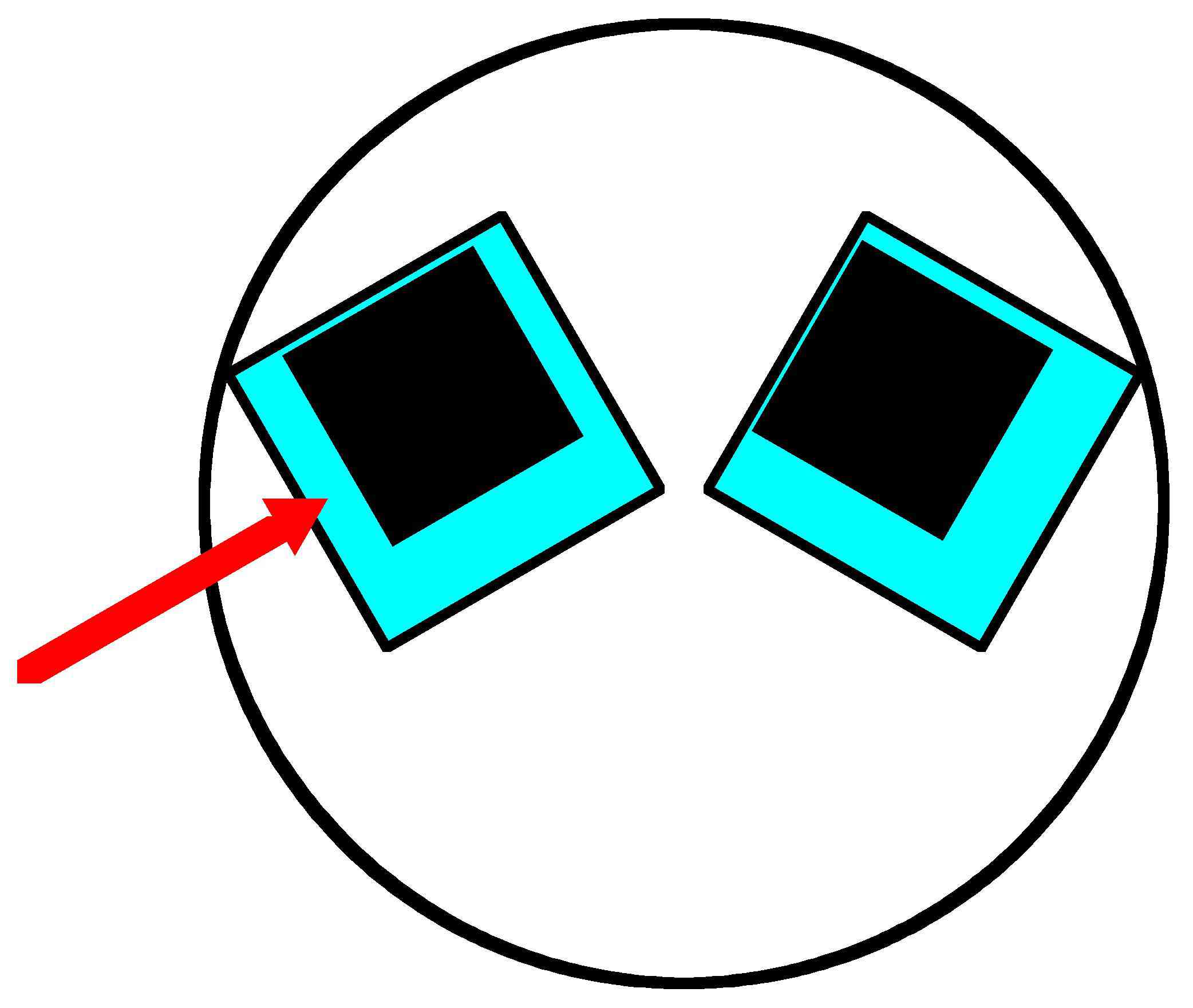
(c)	(d)
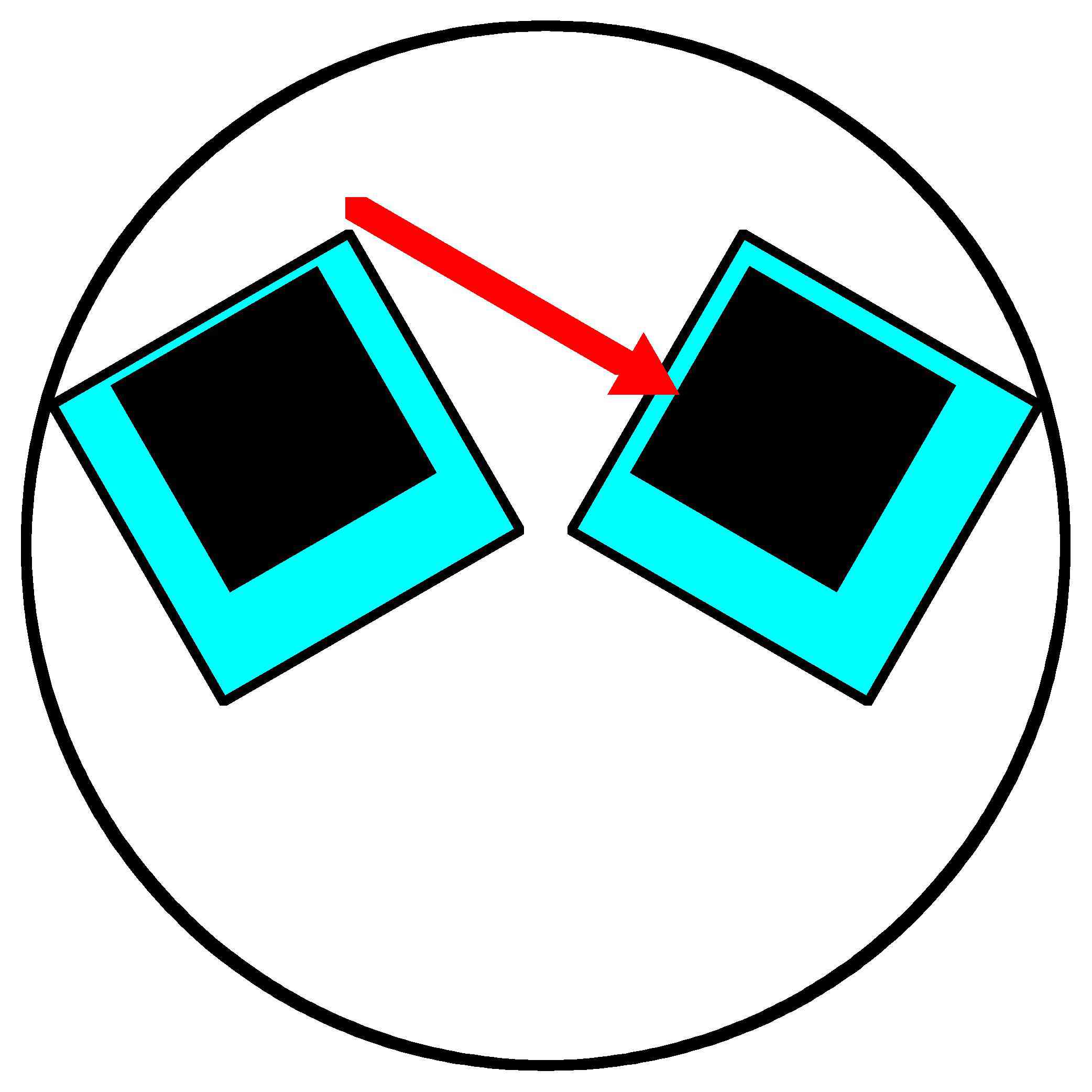
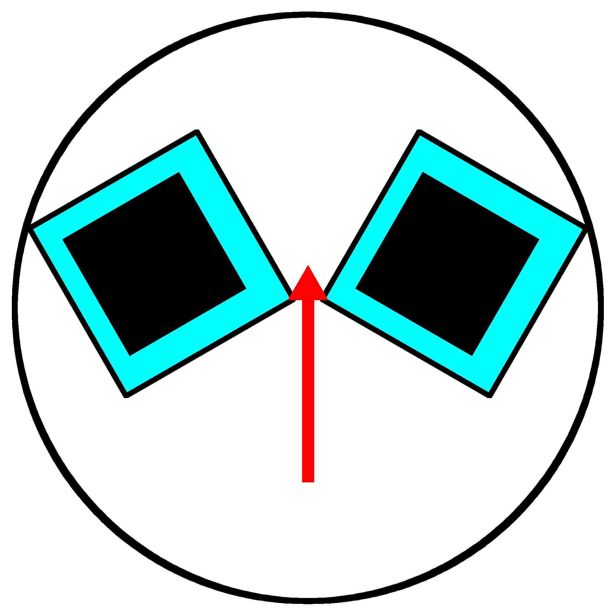
(e)	(f)

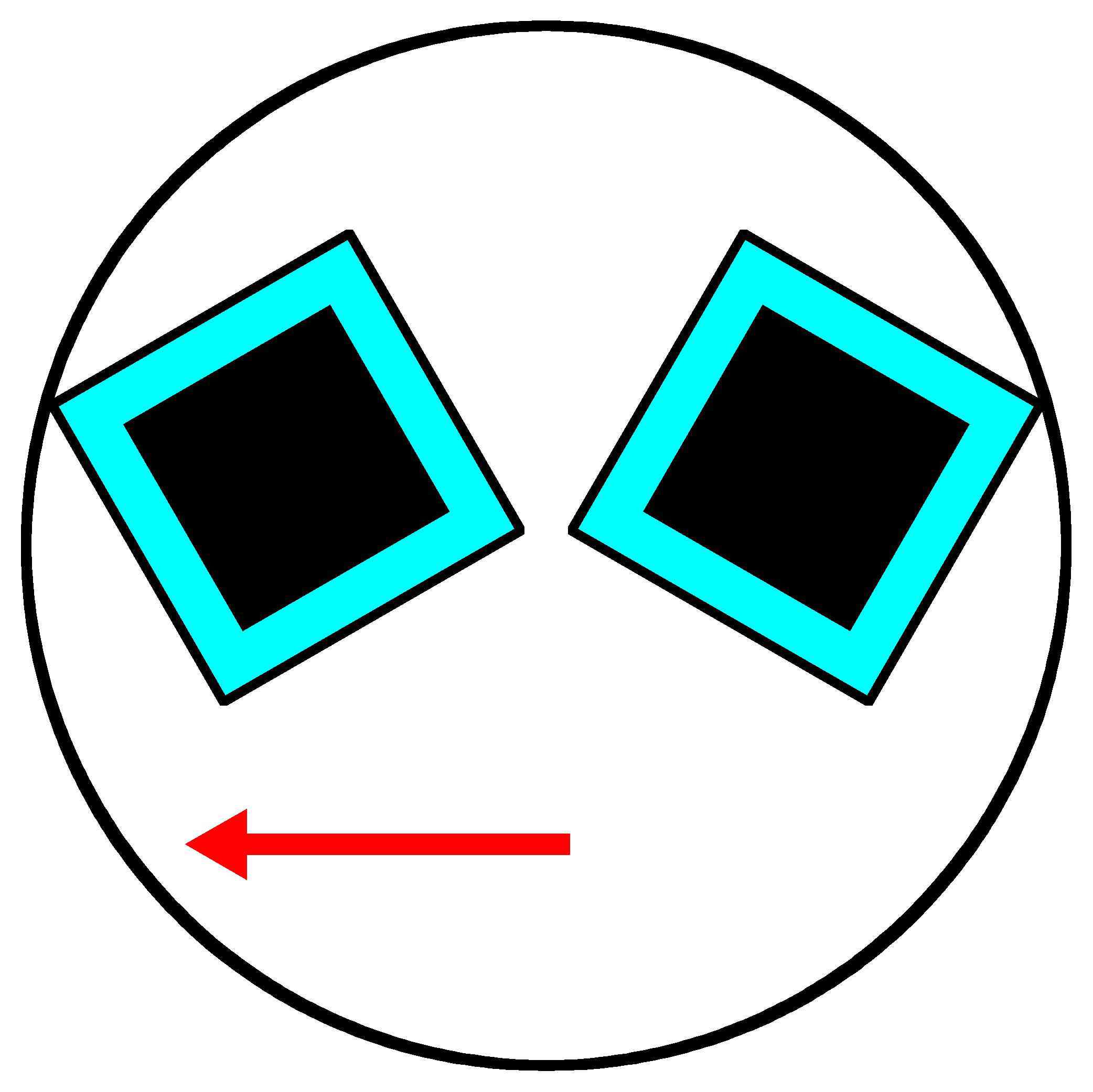
Figure 1.11: LISA’s control strategy per each SC: (a) shows the nominal position of TMs inside the ISs, in (b) the masses get arbitrarily displaced (no rotation for simplicity), on (c) and (d) steps the GRSs actuate the TMs in directions orthogonal to the sensing ones, across (e) and (f) the SC moves to recenter the TMs.

The SCs constellation rotates around its centre of mass on a plane tilted by $\nicefrac{{\pi}}{{3}}\,\mathrm{rad}$ with respect to the ecliptic (see figure 1.9). A clever choice of orbit will allow the formation to complete a full rotation when completing a full revolution around the Sun. Due to the tilting of the rotating plane, the revolution orbit gets eccentric, with a relative factor $e\sim L=D\sqrt{3}\sim 10^{-2}$ and inclination to the ecliptic $\phi=\nicefrac{{L}}{{D}}\sim 1$ degree. This special choice of orbits ensures the triangular geometry of the constellation to remain reliable for a prolonged time over the mission timescale, and the rotation provides some angular resolution. The orbital motion shall induce Doppler shift on the detected signal and modulate its amplitude thus allowing angular definition of the source. LISA’s sources (from very distant massive black holes) should be resolvable to better than an arc-minute; and even the weaker sources (Galactic binaries) should be positioned to within one degree throughout the entire Galaxy. Table 1.1 provides features and numbers of the so called “standard candles” which will be used to calibrate LISA. We strongly point out anyway that once placed on orbit in the proper conditions, LISA will gravitate according to the orbits we described, not much can be done to change or correct it by the controlling thrusters and by itself the constellation will “breathe” radially about some $6\times 10^{4}\,\mathrm{km}$ length. The motion will be anyway at extremely low frequency, well outside the MBW, on the scale of months.

Class	Source	Dist $(\mathrm{pc})$	$f$	$\nicefrac{{M_{1}}}{{M_{\odot}}}$	$\nicefrac{{M_{1}}}{{M_{\odot}}}$	$h$	SNR
WD+WD	WD 0957-666	$100$	$0.38$	$0.37$	$0.32$	$4.00\times 10^{-22}$	$4.1$
	WD1101+364	$100$	$0.16$	$0.31$	$0.36$	$2.00\times 10^{-22}$	$0.4$
	WD1704+481	$100$	$0.16$	$0.39$	$0.56$	$4.00\times 10^{-22}$	$0.7$
	WD2331+290	$100$	$0.14$	$0.39$	$>0.32$	$2.00\times 10^{-22}$	$0.3$
WD+sdB	KPD0422+4521	$100$	$0.26$	$0.51$	$0.53$	$6.00\times 10^{-22}$	$2.9$
	KPD1930+2752	$100$	$0.24$	$0.5$	$0.97$	$1.00\times 10^{-21}$	$4.1$
AM CVn	RXJ0806.3+1527	$300$	$6.2$	$0.4$	$0.12$	$4.00\times 10^{-22}$	$173.2$
	RXJ1914+245	$100$	$3.5$	$0.6$	$0.07$	$6.00\times 10^{-22}$	$195.0$
	KUV05184-0939	$1000$	$3.2$	$0.7$	$0.092$	$9.00\times 10^{-23}$	$27.3$
	AM CV n	$100$	$1.94$	$0.5$	$0.033$	$2.00\times 10^{-22}$	$35.6$
	HP Lib	$100$	$1.79$	$0.6$	$0.03$	$2.00\times 10^{-22}$	$32.0$
	CR Boo	$100$	$1.36$	$0.6$	$0.02$	$1.00\times 10^{-22}$	$10.6$
	V803 Cen	$100$	$1.24$	$0.6$	$0.02$	$1.00\times 10^{-22}$	$9.2$
	CP Eri	$200$	$1.16$	$0.6$	$0.02$	$4.00\times 10^{-23}$	$3.3$
	GP Com	$200$	$0.72$	$0.5$	$0.02$	$3.00\times 10^{-23}$	$1.1$
LMXB	4U1820-30	$8100$	$3$	$1.4$	$<0.1$	$2.00\times 10^{-23}$	$5.7$
	4U1626-67	$<8000$	$0.79$	$1.4$	$<0.03$	$6.00\times 10^{-24}$	$0.2$
W UM a	CC Com	$90$	$0.105$	$0.7$	$0.7$	$6.00\times 10^{-22}$	$0.5$

Table 1.1: LISA calibration binaries. Notice $f=\nicefrac{{2}}{{T}}\,(\mathrm{mHz})$, where $T$ is the period. Signal to noise ratio SNR is averaged over $1\,\mathrm{Year}$.

The TMs relative motion will provide the scientific data, since the masses themselves act as mirrors for the laser light. Each TM will be a $46\,\mathrm{mm}$ sided cube, weighting $1.96\,\mathrm{kg}$, made of Pt-Au alloy to guarantee very low magnetic susceptibility. Weight and sizer are details from the LTP design, but likely to be accepted for LISA as well. By inspection of picture 1.10 the reader might see that each TM is hosted in a separate section of the “Y-tube” as for obvious reasons the internal cavity of LISA is called.

In principle, the SC shall be able to follow both proof-masses with the technique described before. In practise such a picture needs continuous dynamical adjustment: the capacitive sensors forming the GRS system continuously monitor the TMs position with the weakest electrostatic coupling possible, while rotational degrees of freedom are adjusted at low-frequency with the technique of wavefront sensing: each telescope concentrates the light coming from far SCs on a quadrant photo-diode capable of angular resolution of the source and each SC is thus slowly “chasing” the others to reduce minimise variation of the wavefront angle from the nominal value of zero.

The GRS is mounted on the OB, a rigid structure made of ultra-low expansion material, about $350\,\mathrm{mm}$ by $200\,\mathrm{mm}$ by $40\,\mathrm{mm}$. By virtue of optical fibres preserving polarisation the laser light is conducted to the OB after bouncing off the proof mass. Here it is brought to interference with a fraction of the internally generated laser light. As shown, phase noise appears just like a bona-fide GW signal, therefore lasers must be highly efficient, stable in frequency and amplitude. Solid-state diode-pumped monolithic miniature Nd:YAG ring lasers have been chosen for the mission; such a kind of laser generates a continuous $1\,\mathrm{W}$ infrared beam with a wavelength of $1.064\,\mathrm{\mu m}$, relatively immune to refraction by the interplanetary medium. Each SC has two operational $1\,\mathrm{W}$ lasers, one per telescope. One laser is switched on first and acts as matrix: a fraction of its light ($10\,\mathrm{mW}$) is reflected from the back surface of the relative proof mass, and its phase used as a reference for the other local laser.

Hence, the main beams going out along each arm can be considered as a single laser carrier. It is shone through the telescope, which also collects the incoming light from the spare SC. The telescope widens the diameter of the beam from a few $\mathrm{mm}$ to $30\,\mathrm{cm}$. The transmitting and receiving telescopes are improved Cassegrain, including an integral matching lens; both are protected by a thermal shield.

The primary mirror has a diameter of $30\,\mathrm{cm}$ and a focal length of $30\,\mathrm{cm}$. The secondary mirror is mounted $27.6\,\mathrm{cm}$ from the primary and has a diameter of $3.2\,\mathrm{cm}$ and a focal length of $2.6\,\mathrm{cm}$. It is very likely that active focus control will be necessary to compensate for deformations, in case temperature drifts or other phenomena will create any. Notice a change of about one micron already deforms the outgoing wavefront by the specified tolerance $\nicefrac{{f}}{{10}}$, hence the temperature fluctuations at the telescope must be less than $10\,\nicefrac{\mathrm{K}}{\mathrm{Hz}}$ at $10^{-3}\,\mathrm{Hz}$.

Each SC will be disk shaped, carrying surface solar cells: LISA will have constant illumination from the Sun with an angle of $30$ degrees, which in turn provide a very stable environment from the thermal point of view. A set of Field Emission Electric Propulsion (FEEP) devices are employed as thrusters in order to move the SC.

A Delta IV carrier will host the three LISA SCs for launch. After separation from the rocket, the three SCs - equipped with own extra-propulsion rocket - will separate and transfer to solar orbit. Once the constellation is established the propulsion systems are discarded and the FEEPs take over as the only remaining propulsion system.

1.8 The LISA Pathfinder

1.8.1 Noise identification

Achieving pure geodesic motion at the level requested for LISA, $\sqrt{2}\times 3\times 10^{-15}\,\nicefrac{\mathrm{m\,s}}{\mathrm{\sqrt{Hz}}}$ at $0.1\,\mathrm{mHz}$, is considered a challenging technological task [25, 26, 10, 27]. The goal of the SMART-2 test planned by ESA is demonstrate geodetic motion within one order of magnitude from the LISA performance to confirm the formerly elucidated TT-construction and that the shown noise figures are compatible with the LISA demands.

SMART-2 will launch in 2009; on-board the LTP is designed to demonstrate new technologies that have significant application to LISA and other future Space Science missions. Three primary technologies are included on LTP/SMART-2: Gravitational Sensors, Interferometers and Micro-thrusters.

Within the LTP, two LISA-like TMs located inside a single SC are tracked by a laser interferometer. This minimal instrument is deemed to contain the essence of the construction procedure needed for LISA and thus to demonstrate its feasibility. This demonstration requires two steps:

1. first, based on former noise models [28] and the current one in this publication, the mission is designed so that any differential parasitic acceleration noise of the TMs is kept below the requirements. For the LTP these requirements are relaxed to $3\times 10^{-14}\,\nicefrac{\mathrm{m}}{\mathrm{s^{2}\sqrt{Hz}}}$ a factor $\simeq 7$ worse than what is required in LISA. In addition this performance is only required for frequencies larger than $1\,\mathrm{mHz}$:

   $$S^{\nicefrac{{1}}{{2}}}_{\nicefrac{{\Delta F}}{{m}},\,\text{LTP}}(\omega)=3\times 10^{-14}\left(1+\left(\frac{\omega}{2\pi\times 3\,\mathrm{mHz}}\right)^{4}\right)^{\nicefrac{{1}}{{2}}}\,\nicefrac{\mathrm{m}}{\mathrm{s^{2}\sqrt{Hz}}}\,.$$ (1.81)

   This relaxation of performance is accepted since the mission will make use of one single satellite and two probe masses sharing the sensing axis. With such a configuration, actuation is needed to hold one mass and it’s quite unlikely to reach LISA’s precision given actuation and all the disturbances at play. The choice of a single satellite was made in view of cost and time saving. Notice LTP will measure residual acceleration difference between the two TMs, therefore though the deemed precision is reduced by one order of magnitude, the test is highly representative of LISA’s TMs behaviour. Moreover, it would be careless to venture into further design phases of LISA without testing the part of technology which is absolutely mandatory for it to work. The ideal test would imply the use of $2$ SCs to verify drag-free and depict noise in a situation more closely matching LISA’s; nevertheless a single satellite mission would be order of magnitudes cheaper and much less time-consuming on the design front.

   As both for LISA and for the LTP this level of performance cannot be verified on ground due to the presence of the large Earth gravity, the verification is mostly relying on the measurements of key parameters of the noise model of the instrument [22, 29, 23, 30, 31]. In addition an upper limit to all parasitic forces that act at the proof-mass surface (electrostatics and electromagnetics, thermal and pressure effects etc.) has been put and keeps being updated by means of a torsion pendulum test bench [32, 33]. In this instrument a hollow version of the proof mass hangs from the torsion fibre of the pendulum so that it can freely move in a horizontal plane within a housing which is representative of flight conditions. Current limits on torque noise has been measured that would amount to $3\times 10^{-13}\,\nicefrac{\mathrm{m\,s}}{\mathrm{\sqrt{Hz}}}$ [22], when translated into an equivalent differential acceleration. Such a figure is encouraging and calls for an off-ground testing

2. Second, once in orbit the residual differential acceleration noise of the proof masses is measured. The noise model [34, 35] predicts that the total PSD is contributed by sources of three broad categories:

   1. those sources whose effects can be identified and suppressed by a proper adjustment of selected instrument parameters. An example of this is the force due to residual coupling of TMs to the SC. By regulating and eventually matching, throughout the application of electric field, the stiffness of this coupling for both proof masses, this source of noise can be first highlighted, then measured, and eventually suppressed.

   2. Noise sources connected to measurable fluctuations of some physical parameter. Forces due to magnetic fields or to thermal gradients are typical examples. The transfer function between these fluctuations and the corresponding differential proof mass acceleration fluctuations will be measured by purposely enhancing the variation of the physical parameter under investigation and by measuring the corresponding acceleration response: for instance the LTP carries magnetic coils to apply comparatively large magnetic field signals and heaters to induce time varying thermal gradients.

      In addition the LTP also carries sensors to measure the fluctuation of the above physical disturbances while measuring the residual differential acceleration noise in the absence of any applied perturbation. Magnetometers and thermometers, to continue with the examples above. By multiplying the measured transfer function by the measured disturbance fluctuations, an acceleration noise data stream can be computed and subtracted from the main differential acceleration data stream.

      This way the contribution of these noise sources are suppressed and the residual acceleration PSD decreased. This possible subtraction can relax some difficult requirements, like expensive magnetic “cleanliness”, or thermal stabilisation programs.

   3. Noise sources that cannot be removed by any of the above methods. The residual differential acceleration noise must be accounted for by these sources. To be able to do the required comparison, some of the noise model parameters must and will be measured in flight. One example for all, the charged particle flux due to cosmic rays will be continuously monitored by a particle detector.

The result of the above procedure is the validation of the noise model for LISA and the demonstration that no unforeseen source of disturbance is present that exceeds the residual uncertainty on the measured PSD. The following sections, after describing some details of the experiment, will discuss the expected amount of this residual uncertainty.

1.8.2 The instrument

The basic scheme of the LTP [27] is shown in figure 1.12: two free floating TMs are hosted within a single SC and the relative motion along a common sensitive axis, the $\hat{x}$-axis, is measured by means of a laser interferometer. The TMs are made of a Gold-Platinum, low magnetic susceptibility alloy, have a mass of $m=1.96\,\mathrm{kg}$ and are separated by a nominal distance of $0.376\,\mathrm{m}$.

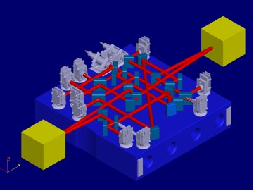
Figure 1.12: The concept of the LTP. The distance between 2 cubic, free floating TMs is measured by a heterodyne laser interferometer. Each proof mass is surrounded by a set of electrodes that are used to readout the mass position and orientation relative to the SC. This measurement is obtained as the motion of the proof mass varies the capacitance’s between the electrodes and the proof mass itself. The same set of electrodes is also used to apply electrostatic forces to the TMs.

Differential capacitance variations are parametrically read out by a front end electronics composed of high accuracy differential inductive bridges excited at about $100\,\mathrm{kHz}$, and synchronously detected via a phase sensitive detector [36, 14]. Sensitivity depends on the DOF: for the $\hat{x}$-axis it is better than $1.8\,\nicefrac{\mathrm{nm}}{\mathrm{\sqrt{Hz}}}$ at $1\,\mathrm{mHz}$. Angular sensitivities are better than $200\,\nicefrac{\mathrm{nrad}}{\mathrm{\sqrt{Hz}}}$. Forces and torques on the TMs required during science operation are applied through the same front end electronics by modulating the amplitude of an ac carrier applied to the electrodes. The frequency of the carrier is high enough to prevent the application in the measurement band of unwanted forces by mixing with low frequency fluctuating random voltages. The front end electronics is also used to apply all voltages required by specific experiments. Each proof mass, with its own electrode housing, is enclosed in a high vacuum chamber which is pumped down to $10^{-5}\,\mathrm{Pa}$ by a set of getter pumps. The laser interferometer light crosses the vacuum chamber wall through an optical window.

As the proof mass has no mechanical contact to its surrounding, its electrical charge continues to build up due to cosmic rays. To discharge the proof mass, an ultra violet light is shone on it and/or on the surrounding electrodes [37]. Depending on the illumination scheme, the generated photo-electrons can be deposited on or extracted from the proof mass to achieve electrical neutrality. The absence of a mechanical contact also requires that a blocking mechanism keep the mass fixed during launch and is able to release it once in orbit, overcoming the residual adhesion. This release must leave the proof mass with low enough linear momentum to allow the control system described in the following to bring it at rest in the nominal operational working point. The system formed by one proof mass, its electrode housing, the vacuum enclosure and the other subsystems is called in the following the gravity reference sensor.

The interferometer system includes many measurement channels. It provides:

1. heterodyne measurement of the relative position of TMs along the sensitive axis.

2. Heterodyne measurement of the position of one of the proof-masses (proof mass 1) relative to the optical bench.

3. Differential wave front sensing of the relative orientations of the proof-masses around the $\hat{y}$ and $\hat{z}$ axes.

4. Differential wave front sensing of the orientation of proof-mass 1 around the $\hat{y}$ and $\hat{z}$ axes.

Sensitivities at $\mathrm{mHz}$ frequency are in the range of $10\,\nicefrac{\mathrm{pm}}{\mathrm{\sqrt{Hz}}}$ for displacement and of $10\,\nicefrac{\mathrm{nrad}}{\mathrm{\sqrt{Hz}}}$ on rotation. Interferometry is performed by a front-end electronics largely based on Field Programmable Gate Arrays. Final combination of phases to produce motion signals is performed by the LTP instrument computer. The LTP computer also drives and reads-out the set of subsidiary sensors and actuators needed to apply the already mentioned selected perturbations to the TMs and to measure the fluctuations of the disturbing fields. Actuators include coils used to generate magnetic field and magnetic field gradients and heaters to vary temperature and temperature differences at selected points of the Gravity Reference Sensor and of the optical bench. Sensors include magnetometers, thermometers, particle detectors and monitors for the voltage stability of the electrical supplies.

LTP will be hosted in the central section of the SC (see figure 1.13, left), where gravitational disturbances are minimised, and will operate in a Lissajous orbit (see figure 1.13, right and figure 1.14) [38] around the Lagrange point 1 of the Sun-Earth system.

Figure 1.13: Left: the LTP accommodated within the central section of the LISA Pathfinder SC. Right: the injection of LISA Pathfinder in the final orbit around L1.

Figure 1.14: Lissajous orbit for LTP around L1.

1.8.3 A simplified model

The sensitivity performance estimated before is limited at low frequencies by stray forces perturbing the TMs out of their geodesics. Better would be to say that the presence of perturbations due to non-gravitational interactions in the energy-momentum tensor generates a deformed geometry in space-time, thus perturbing the “natural” geodesics the TMs would follow in vacuo.

In contrast with the usual view of a space-probe dragging along its content, drag-free reverses the scenario and it’s the TMs inside the satellite which dictate the motion of the latter.

Figure 1.15: Simple scheme of LTP.

Figure 1.16: Spring and particles model for LTP.

To illustrate the features of drag-free technique and relative detectable signals, we proceed now to illustrate a simple one-dimensional model of two TMs coupled to a SC. Let $m$ be each TM mass, $m_{\text{SC}}$ the SC mass, $k_{i}$, $i=1,2$ two spring constants summarising the Hooke-like coupling of the various masses. We let external forces, generally named after $f_{i,x}$, with $i=1,2,\text{SC}$ act on the respective body. By Newton’s law, the dynamics can be written as:

$$m\ddot{x}_{1}+k_{1}\left(x_{1}-x_{\text{SC}}\right) =f_{1,x}\,,$$ (1.82)

$$m\ddot{x}_{2}+k_{2}\left(x_{2}-x_{\text{SC}}\right) =f_{2,x}\,,$$ (1.83)

$$m_{\text{SC}}\ddot{x}_{\text{SC}}-k_{1}\left(x_{1}-x_{\text{SC}}\right)-k_{2}\left(x_{2}-x_{\text{SC}}\right) =f_{\text{SC},x}\,.$$ (1.84)

Each force can be thought as a force per unit mass $m$ and separated into an external contribution and a feed-back term, accounting for our desire to realise a mechanical control loop:

$$\begin{split}f_{1,x}\to m\left(g_{1,x}+g_{\text{fb1},x}\right)\,,\\ f_{2,x}\to m\left(g_{2,x}+g_{\text{fb2},x}\right)\,,\\ f_{\text{SC},x}\to m_{\text{SC}}\left(g_{\text{fbSC},x}+g_{\text{SC},x}\right)\,,\end{split}$$ (1.85)

here $g_{i,x},\,i=1,2,\text{SC}$ is the external acceleration acting on the $i$-th TM or on the SC, while $g_{\text{fb}i,x}$ is the feed-back force per unit mass we’d like to apply to realise a certain control strategy. Moreover, couplings can be translated into elastic stiffness terms, per unit mass, being the DOF at play linear:

$$k_{i}\to m\omega_{p,i}^{2}\,,\qquad i=1,2\,.$$ (1.86)

We’ll work in the approximation of very large SC mass, and introduce a mass scale parameter $\mu$ as follows:

$$\mu=\frac{m}{m_{\text{SC}}}\,.$$ (1.87)

Every uncertainty in the TMs position or every deformation of the bench hosting optical or electrostatic measuring device may induce undesired error in position detection and will be summarised into two ${\delta}x_{i}$ ($i=1,2$) variables, so that in the equations of motion and in the feed-back laws the following substitution will take place:

$$x_{i}\to x_{i}+{\delta}x_{i}\,,\qquad i=1,2\,.$$ (1.88)

Notice we’ll assume these deformations to be stationary, to get ${\delta}\dot{x}_{i}\simeq 0$. Anyway materials will always be chosen so to ensure these deformation to be small with respect to displacement, in spectral form:

$$S_{{\delta}x_{i}}^{\nicefrac{{1}}{{2}}}\ll S_{x_{i}}^{\nicefrac{{1}}{{2}}}\,.$$ (1.89)

Finally, we’ll work in Laplace space from now on, and make the substitution:

$$\frac{\operatorname{d}x_{i}}{\operatorname{d}t}\to sx_{i}\,,\qquad i=1,2\,,$$ (1.90)

when needed. In turn, we’ll switch to Fourier space by placing $s\doteq-\imath\omega$. Finally, the equations of motion display like:

$$-mx_{1}\omega^{2}+m\left(x_{1}-x_{\text{SC}}+{\delta}x_{1}\right)\omega_{p,1}^{2} =mg_{1,x}+mg_{\text{fb1},x}\,,$$ (1.91)

$$-mx_{2}\omega^{2}+m\left(x_{2}-x_{\text{SC}}+{\delta}x_{2}\right)\omega_{p,2}^{2} =mg_{2,x}+mg_{\text{fb2},x}\,,$$ (1.92)

$$-\frac{m}{\mu}x_{\text{SC}}\omega^{2}-m\left(x_{1}-x_{\text{SC}}+{\delta}x_{1}\right)\omega_{p,1}^{2}-m\left(x_{2}-x_{\text{SC}}+{\delta}x_{2}\right)\omega_{p,2}^{2} =\frac{m}{\mu}g_{\text{fbSC},x}+\frac{m}{\mu}g_{\text{SC},x}\,.$$ (1.93)

A drag-free strategy is a map whose task is enslaving the satellite motion to the TMs. This can be achieved in many ways, but since it’s impossible to follow the motion of both TMs along one common axis, two strategies are left unique as solutions:

1. the SC follows TM1, and TM2 is held in position by continuously servoing its position with respect to the SC itself, i.e. for our simple system:

   $$\begin{split}g_{\text{fb1},x}&\to 0\,,\\ g_{\text{fb2},x}&\to-\left(x_{2}-x_{\text{SC}}+x_{n,2}\right)\omega_{\text{lfs},x}^{2}\,,\\ g_{\text{fbSC},x}&\to\left(x_{1}-x_{\text{SC}}+x_{n,1}\right)\omega_{\text{df},x}^{2}\,,\end{split}$$ (1.94)

   where we introduced “position readout” noise for the channels $x_{1}$ and $x_{2}$ and named it $x_{n,1}$ and $x_{n,2}$ respectively. We may think of this noise as being provided by some electrostatic readout circuitry. We also decided to complicate our picture by taking control of the “gain” of the feed-back: instead of being $1$, the multiplication constant is a function of the complex frequency, namely $\omega_{\text{lfs},x}^{2}(s)$, LFS meaning “low frequency suspension” and $\omega_{\text{df},x}^{2}(s)$, DF meaning “drag-free”.

2. On the other hand, we may choose to pursue TM1 with the SC and to hold TM2 fixed on the distance to TM1 itself, in formulae:

   $$\begin{split}g_{\text{fb1},x}&\to 0\,,\\ g_{\text{fb2},x}&\to-\left(x_{2}-x_{1}+{\Delta}x_{n}\right)\omega_{\text{lfs},x}^{2}\,,\\ g_{\text{fbSC},x}&\to\left(x_{1}-x_{\text{SC}}+x_{n,1}\right)\omega_{\text{df},x}^{2}\,,\end{split}$$ (1.95)

   where now the new noise ${\Delta}x_{n}$, typical of the difference channel, was introduced

If we’d choose the first approach, we could solve the equations of motion in the approximation of $\mu\to 0$. Moreover, we can decide to take a very severe drag-free control policy, and take also $\left|\omega_{\text{df},x}^{2}\right|\gg\left|\omega^{2}\right|$ and larger than every other frequency at play. The solution of the problem is analytic but quite tedious - it can be computed with the help of any symbolic algebraic program - and we’ll state here only the result for the main difference channel as function of $\omega$:

$$\begin{split}x_{2}-x_{1}+{\Delta}x_{n}\underset{\begin{subarray}{c}\mu\to 0\\ \omega_{\text{df},x}^{2}\to\infty\end{subarray}}{\simeq}\frac{1}{-\omega^{2}+\omega_{\text{p},2}^{2}+\omega_{\text{lfs},x}^{2}}\Bigl{(}&-x_{n,2}\omega_{\text{lfs},x}^{2}+g_{2,x}-g_{1,x}+\\ &+\left({\delta}x_{1}-{\delta}x_{2}\right)\left(\omega_{\text{p},2}^{2}+\omega_{\text{lfs},x}^{2}\right)+\\ &+\left(x_{n,1}+\frac{g_{\text{SC},x}}{\omega_{\text{df},x}^{2}}\right)\left(-\omega_{\text{p},1}^{2}+\omega_{\text{p},2}^{2}+\omega_{\text{lfs},x}^{2}\right)\Bigr{)}+\\ &+{\Delta}x_{n}\,.\end{split}$$ (1.96)

Furthermore, in the approximation of very low frequency suspension $\omega_{\text{lfs},x}^{2}$ to compensate the intrinsic static stiffness $\omega_{\text{p},2}^{2}$, we may think the following approximations to hold. Notice $\omega_{\text{p},2}^{2}\simeq 2\times 10^{-6}$ is a believable value for the parasitic stiffness [26], versus $\omega_{\text{lfs},x}^{2}$ whose value must be kept small or it would amplify the noise source represented by $\sim\omega_{\text{lfs},x}^{2}\left(x_{n,1}+\nicefrac{{g_{\text{SC},x}}}{{\omega_{\text{df},x}^{2}}}\right)$ which might in turn become dominant over the rest of the expression (1.96). Keeping $\left|\omega_{\text{lfs},x}^{2}\right|\ll\left|\omega_{\text{p},2}^{2}-\omega_{\text{p},1}^{2}\right|$ prevents that every time the SC suffers jitter or displacement - be it unwilling or induced by thrusters - the same shaking won’t affect the TM due to the tight coupling. Conversely, the value of $\left|\omega_{\text{lfs},x}^{2}\right|$ must be kept $\simeq 2\left|\omega_{\text{p},2}^{2}\right|$ to achieve control stability (the LFS acts as a positive spring whose value must be double the negative one to compensate for). As we can see, a delicate balance is at play. Finally over a large scale of frequencies, $\omega$ is larger than the parasitic couplings and the feed-back gains but the drag-free (MBW, $10^{-3}\,\mathrm{Hz}\leq\nicefrac{{\omega}}{{2\pi}}\leq 1\,\mathrm{Hz}$):

$$\omega^{2}\gg\left|\omega_{\text{p},2}^{2}+\omega_{\text{lfs},x}^{2}\right|\,.$$ (1.97)

In summary, the front filter becomes:

$$\frac{1}{-\omega^{2}+\omega_{\text{p},2}^{2}+\omega_{\text{lfs},x}^{2}}\simeq\frac{1}{-\omega^{2}}\,,$$ (1.98)

and in the end:

$$\begin{split}x_{2}-x_{1}+{\Delta}x_{n}\underset{\left|\omega^{2}\right|\gg\left|\omega_{\text{lfs},x}^{2}+\omega_{\text{p},2}^{2}\right|}{\simeq}-\frac{1}{\omega^{2}}\Bigl{(}&-x_{n,2}\omega_{\text{lfs},x}^{2}+g_{2,x}-g_{1,x}+\\ &+\left({\delta}x_{1}-{\delta}x_{2}\right)\left(\omega_{\text{p},2}^{2}+\omega_{\text{lfs},x}^{2}\right)+\\ &+\left(x_{n,1}+\frac{g_{\text{SC},x}}{\omega_{\text{df},x}^{2}}\right)\left(\omega_{\text{p},2}^{2}-\omega_{\text{p},1}^{2}+\omega_{\text{lfs},x}^{2}\right)\Bigr{)}+{\Delta}x_{n}\,.\end{split}$$ (1.99)

In the limit of very low coupling this control mode has thus a natural self-calibration property between force and displacement signal, being purely inverse proportional to the frequency squared. Undoubtedly, this feature may be of great use in absence of deep knowledge on a more complicated device with many DOF. In chapter 2 we’ll complicate this simple model and the special character of this mode will be discussed and employed. We’ll call this mode “nominal” (formerly M1) and will discuss it thoroughly in section 2.4 and 2.4.2.

The mentioned signal is anyway a good estimator of the acceleration difference acting on the TMs: $g_{2,x}-g_{1,x}$, provided a good matching of LFS and parasitic stiffness could be performed $\left(\omega_{\text{lfs},x}^{2}\simeq\omega_{\text{p},2}^{2}\right)$ and drag-free gain could damp SC jitter to a good level $\left(\nicefrac{{g_{\text{SC}}}}{{\omega_{\text{df},x}^{2}}}\ll 1\right)$.

Notice, conversely, that this readout signal carries along the ${\Delta}x_{n}$ noise term fully unabridged, independent on the frequency applied. It is therefore transparent that this mode will be intrinsically noisier than other solutions unless we guarantee that ${\Delta}x_{n}\ll x_{n,i}$, another point to choose interferometer detection for mutual displacement of the TMs.

Equal coupling of the two TMs to the SC can result in a “common mode” excitation as response of the two masses. As an effect, the high-sensitivity interferometric signal will be rendered blind by the coupled dynamics. The optimal feedback $\omega_{\text{lfs},x}^{2}$ is designed to unbalance the coupling acting as a control spring and giving a differential coupling like

$$\left|\omega_{\text{p},1}^{2}-\left(\omega_{\text{p},2}^{2}+\omega_{\text{lfs}}^{2}\right)\right|\simeq 2\left|\omega_{\text{p},2}^{2}\right|\,.$$ (1.100)

This differential coupling may be measured by modulating the drag-free control set-point and tuned via $\omega_{\text{lfs},x}^{2}$ to distinguish SC coupling noise from random force noise.

This control mode may present very large mechanical transients (long relaxation time for TM2 motion to stabilise), since $\left|\omega_{\text{lfs},x}^{2}\right|$ cannot be tightened, for all the mentioned motivations. Therefore this mode might have very poor experimental times, the largest part of it being wasted.

In LISA one single direction will be pursued by the SC, i.e. the mid-line between the directions spanned by the optical sensing lines. It is impossible to pursue both the TMs in LTP, being they coaxial along the sensing direction, as stated. Nevertheless this control mode is highly representative of LISA, whose dynamical picture we shall mimic at maximal level to gain knowledge about forces and noise behaviour [26, 39].

If conversely we’d use the locking onto the $x_{2}-x_{1}$ distance, in the usual $\mu\to 0$ and high drag-free gain approximations, we’d find for the distance signal itself:

$$\begin{split}x_{2}-x_{1}+{\Delta}x_{n}\simeq\frac{1}{\omega_{\text{lfs},x}^{2}+\omega_{\text{p},2}^{2}-\omega^{2}}\Bigl{(}&\left(\omega_{\text{p},2}^{2}-\omega^{2}\right){\Delta}x_{n}+g_{2,x}-g_{1,x}+\\ &+\left(\omega_{\text{p},2}^{2}-\omega_{\text{p},1}^{2}\right)\left(x_{n,1}+\frac{g_{\text{SC},x}}{\omega_{\text{df},x}^{2}}\right)\\ &+\left({\delta}x_{1}-{\delta}x_{2}\right)\left(\omega_{\text{p},2}^{2}+\omega_{\text{lfs},x}^{2}\right)\Bigr{)}\,.\end{split}$$ (1.101)

In this case, apart from fulfilling stability issues the value of $\left|\omega_{\text{lfs},x}^{2}\right|$ doesn’t need to be small since it doesn’t amplify any noise or jitter apart $\left|{\delta}x_{2}-{\delta}x_{1}\right|$. Since the deformations difference $\left|{\delta}x_{2}-{\delta}x_{1}\right|$ may be thought as small [25], the signal is a very good estimator of the distance $x_{2}-x_{1}$ as function of the acceleration difference $g_{2,x}-g_{1,x}$.

This mode doesn’t allow for self-calibration, but the instrumental noise can be modulated by the frequency and the intrinsic stiffness difference is a constant independent of frequency itself, highly damped by DF gain. It is therefore an extremely clean mode as for readout: no LFS gain appears in the noise sources on the r.h.s. of the expression, only as a global tuning term in the foremost propagator. Strengthening the grip of the low frequency suspension is henceforth a technique to damp TM2 motion which may be applied at will within common-sense boundaries. On this side, this control mode won’t waste experimental time in waiting for transients to elapse.

By electrostatically tuning $\omega_{\text{p},1}^{2}\simeq\omega_{\text{p},2}^{2}$ a source of noise characteristic of LISA will be annihilated, i.e.

$$\left(\omega_{\text{p},2}^{2}-\omega_{\text{p},1}^{2}\right)\left(x_{n,1}+\frac{g_{\text{SC},x}}{\omega_{\text{df},x}^{2}}\right)\simeq 0\,,$$ (1.102)

this configuration allows for a clear measurement of $g_{2,x}-g_{1,x}$; in turn, alien noise sources can then be mapped and henceforth subtracted.

In a word in this control mode the mutual distance between the test-masses is held constant. This laser-locking procedure will be much less noisy than the nominal one and is hence defined as “science” mode. The main interferometer signal booking the distance variation between the masses is used and its value kept fixed: no need for the satellite to fire the thrusters as the displacement measurement can be deduced from the applied actuation gains. Besides, the drawback of this mode is the more complicated transfer function from displacement to force to real pull on the SC, a feature which demands precise calibration.

We point out the equivalence between measuring the real laser phase variation (or voltage variation on the capacitors) holding one mass and letting the other fly, and measuring the variation in electrostatic force needed to hold both the masses in position while keeping their distance fixed. In one case, a direct measurement of distance variation is done, on the other is the force needed to compensate for the motion which is estimated.

This simple model shall motivate and guide the reader in venturing into the LTP dynamics chapter and understanding the main characters of drag-free on a simplified canvas.

One last remark at this basic level is of course about low frequency noise. When the controls are forced to exert a direct, non-alternate current in-band via the capacitors, there the noisiest contribution shows up. We remind to chapter 3 for a thorough explanation, but here we can say that with an electrostatic sensor, applying a force also induces a gradient and thus a spring which couples any relative motion into a noisy force: whenever additional, spurious or constant accelerations arise, these need to be compensated and the price to pay for a dynamical, electrostatic compensation is the increase of the coupling between mass and SC, quadratic in the voltage. It is true on the converse that there’s need of a positive spring mechanism to stabilise the dynamics. This aim can be pursued only via a low frequency suspension applied through the electrostatics.

In addition to the electrostatic actuation stiffness, one of the most dangerous sources of DC forces aboard SMART-2 is the action of static self-gravity of the space-probe itself. The presence of uncompensated local static gravity pulls would force the electrostatic system to exert continuous, noisy DC anti-forces [7]. Basic requirements and a full gravitational control protocol [8] have been written to pave the way and solve this delicate issue for both LTP and LISA. A dedicated section of this thesis summarises the large load of work carried on to study the problem of gravitational compensation, the reader may find about it in section 4.2.

1.8.4 Experiment performance and sensitivity, similarities and differences with LISA.

By virtue of a control scheme similar to that we described LISA’s SCs actively follow the proof mass located within each of them. If the loop gain is high enough, the difference in acceleration between two masses sitting in two different SCs can be measured by the interferometer as:

$${\Delta}a={\Delta}g-\omega_{p,2}^{2}{\delta}x_{2}+\omega_{p,1}^{2}{\delta}x_{1}+\omega^{2}{\Delta}x_{n}\,,$$ (1.103)

where $\Delta g$ is the difference of position independent, fluctuating forces per unit mass directly acting on TMs and $\omega_{p,i}^{2}\,i=1,2$ is the stiffness per unit mass of parasitic spring coupling proof mass 1(2) to the SC. ${\delta}x_{i}\,i=1,2$ is the residual jitter of the same proof-mass relative to the SC. Here as before ${\Delta}x_{n}\sim\text{IFO}_{n}({\Delta}x)$ is typically the interferometer noise difference along the $\hat{x}$ channel.

As we saw the LTP experiment uses a similar drag free control scheme. However here both masses sit in one SC and cannot be simultaneously followed by. We saw formerly two control schemes and we refer to the dynamics and noise sections for detailed equations including all DOF and cross-talk.

In the LTP both TMs are spring coupled to the same SC and both feel then the relative jitter between this one and the drag free reference proof mass 1. Therefore we can restate the problem by including this modification together with the effect of the control loop transfer function, recapping (1.101) by means of (1.102):

$${\Delta}a\simeq\frac{\omega^{2}}{\omega_{\text{lfs},x}^{2}+\omega_{\text{p},2}^{2}-\omega^{2}}\Bigl{(}-\omega^{2}{\Delta}x_{n}+{\Delta}g+\left({\delta}x_{1}-{\delta}x_{2}\right)\left(\omega_{\text{p},2}^{2}+\omega_{\text{lfs},x}^{2}\right)\Bigr{)}\,.$$ (1.104)

By setting $\omega^{2}_{p,1}\simeq\omega^{2}_{p,2}$ a substantial residual jitter ${\delta}x_{1}$ might get unobserved thus bringing to optimistic underestimate of the noise in (1.103). This is easily avoided by a detailed sequence of measurements of both $\omega^{2}_{p,1}$ and $\omega^{2}_{p,2}$ that has been described [34]. Provided this procedure, the measure of ${\Delta}g$ can be carried on successfully.

Correlation of disturbances on different proof-masses may play a different role in LISA than in LTP. In LISA proof-masses within the same interferometer arm belong to different SCs and are located $5\times 10^{9}\,\mathrm{m}$ apart. The only correlated disturbances one can think of are connected to the coupling to Sun: magnetic field fluctuations, fluctuation of the flux of charged particles in solar flares and the fluctuation of solar radiation intensity that may induce correlated thermal fluctuations in distant SC. These correlations will only slightly affect the error budget and will have no profound consequences on the experiment itself.

In the LTP all sources of noise that share the same source for both TMs are correlated. Magnetic noise generated on board the SC, thermal fluctuations and gravity noise due to thermo-elastic distortion of SC constitute a few examples. The major concern with correlated noise is that, by affecting the proof-masses the same way, it might subtract from the differential measurement. Such a subtraction would not occur in LISA and thus would bring to an optimistic underestimate of the total noise by LTP. This possibility can reasonably be avoided for almost all candidate effects by a careful study (like the following, see chapter 3) and dedicated procedures.

An exception is constituted by the gravitational noise for which the response, due to the equivalence principle, cannot be changed. However realistic assumptions about thermal distortion make the event of a gravity fluctuation affecting both proof-masses with the same force along the $\hat{x}$ axis very unlikely. Moreover, the TMs are localised and receive pulls by localised mass distributions as well, therefore is quite likely that we’ll have different static components per unit mass.

As an instrument to measure ${\Delta}g$, the LTP is then limited at high frequency by the laser interferometer noise. For this last the laser path length noise is still $S_{{\delta}x}^{\nicefrac{{1}}{{2}}}\leq 20\,\nicefrac{\mathrm{pm}}{\mathrm{\sqrt{Hz}}}$ while the interferometric apparatus is deemed to achieve a sensitivity of:

$$S_{{\delta}x,\,\text{LTP}}^{\nicefrac{{1}}{{2}}}=9\left(1+\left(\frac{\omega}{2\pi\times 3\,\mathrm{mHz}}\right)^{-4}\right)^{\nicefrac{{1}}{{2}}}\,\nicefrac{\mathrm{pm}}{\mathrm{\sqrt{Hz}}}\,,$$ (1.105)

which can be converted into an acceleration noise as before, by virtue of (1.69). In the MBW we don’t really need to be so strict to ask such a complicated function of $\omega^{2}$, more than enough is the effective behaviour:

$$\begin{split}S_{\nicefrac{{{\Delta}F}}{{m}},\,\text{laser, LTP}}^{\nicefrac{{1}}{{2}}}&=\frac{\omega^{2}}{\sqrt{2}}S_{{\delta}x,\,\text{LTP}}^{\nicefrac{{1}}{{2}}}=\\ &\simeq 3.2\times 10^{-15}\left(1+\left(\frac{\omega}{2\pi\times 3\,\mathrm{mHz}}\right)^{2}\right)\,\nicefrac{\mathrm{m}}{\mathrm{s^{2}\sqrt{Hz}}}\,.\end{split}$$ (1.106)

At lower frequencies an additional force noise adds up to mask the parasitic forces due to other sources. This force noise is due to the fluctuations of the gain of the electrostatic suspension loop. Indeed the electrostatic suspension must also cope with any static force acting on the TMs. If the force stays constant but the gain fluctuates, the feedback force fluctuates consequently, adding a noise source that is expected to limit the sensitivity at the lowest frequencies. This effect only appears in the LTP as in LISA static forces are compensated just by the drag-free loop, and no electrostatic suspension is envisaged. The largest expected source of gain fluctuations is the fluctuation of the DC voltage which is used to stabilise the actuation electronics.

Stability should not worsen faster than $\nicefrac{{1}}{{\omega}}$ at lower frequencies down to $0.1\,\mathrm{mHz}$. If this goal can be reached, suspension gain fluctuations may be modelled with the following PSD [10]:

$$S^{\nicefrac{{1}}{{2}}}_{\nicefrac{{{\Delta}F}}{{m}},\,\text{susp, LTP}}\simeq 1.8\times 10^{-15}\nicefrac{\mathrm{m}}{\mathrm{s^{2}\sqrt{Hz}}}\left(1+\left(\frac{\omega}{2\pi\times 1\,\mathrm{mHz}}\right)^{-2}\right)\,.$$ (1.107)

The effective sensitivity curve of LTP - at the level we want to introduce it here - is thus obtained combining (1.106) with (1.107):

$$S_{\nicefrac{{{\Delta}F}}{{m}},\,\text{sens, LTP}}\simeq S_{\nicefrac{{{\Delta}F}}{{m}},\,\text{laser, LTP}}+S_{\nicefrac{{{\Delta}F}}{{m}},\,\text{susp, LTP}}\,.$$ (1.108)

More will be said on noise in chapter 3, here we’d like to give some flavour by showing a sensitivity prediction figure, obtained by plotting $S_{\nicefrac{{{\Delta}F}}{{m}},\,\text{sens, LTP}}^{\nicefrac{{1}}{{2}}}$ with the requirement expressions for LISA, eq. (1.72) and for LTP, eq. (1.81): see figure 1.17.

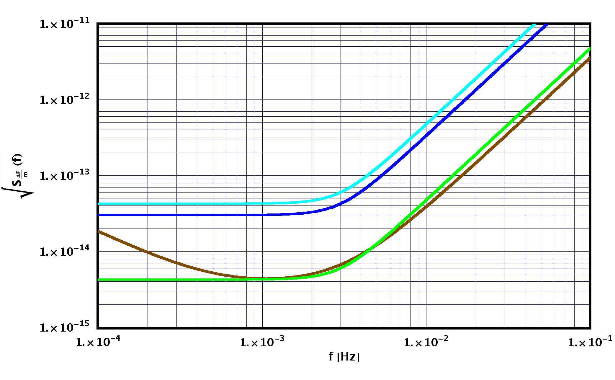
Figure 1.17: Brown curve: projected sensitivity for differential force measurement of the LTP experiment, $S_{\nicefrac{{{\Delta}F}}{{m}},\,\text{sens, LTP}}^{\nicefrac{{1}}{{2}}}$. Blue: required maximum differential acceleration noise for the LTP. Green: LISA requirements. Cyan: LISA minimum mission requirements.

Figure 1.17 shows that the ultimate uncertainty on the differential acceleration PSD can be potentially constrained by the LISA Pathfinder mission below a factor $5$ above LISA requirements at $0.1\,\mathrm{mHz}$, and near LISA requirements at $1\,\mathrm{mHz}$ or above. In addition, within the entire frequency range, the LISA Pathfinder mission will constrain the acceleration noise somewhere in the range between $1$ and $10\,\nicefrac{\mathrm{fm}}{\mathrm{s^{2}\sqrt{Hz}}}$ well below the requirements of LISA minimum mission, thus strongly reducing the risk of a LISA failure. Notice that the resulting TT frame, a frame where free particles at rest remain at rest, is a very close approximation to the classical concept of inertial frame, and would indeed be inertial, within the MBW, wouldn’t it be for the presence of the gravitational wave. Thus LISA Pathfinder will demonstrate the possibility of building an inertial frame in a standard SC orbiting the Sun on a scale of a meter in space and of a few hours in time at the above mentioned level of absence of spurious accelerations.

Chapter 2 LTP: dynamics and signals

Having inspected the main peculiarities of the simplified model for the LTP dynamics in chapter one, we’ll now proceed from ground up in writing down the full LTP dynamics. The purpose is elucidate the procedure of building the signals and motivate control modes from the signals themselves.

Reference systems will be conjured, pictures and renderings of the devices will be provided. The equations of motion have been deduced using Newtonian dynamics. Perhaps a Lagrangian treatment would have been more elegant, but we thought it better to choose the former because noise and feedback are more natural to be introduced in this scenario.

Special cases for the signals have been singled out and a “propagator”-like approach chosen for transfer functions. Feed-backs and suspensions are discussed and their graphical behaviour sketched. The chapter is somehow thought as preparatory for the noise detailed treatment which follows.

2.1 Layout, coordinates and frames

Our concept of LTP to start with is somehow idealised in comparison to reality. Nevertheless the model can be complicated up to whatsoever detail level, by introducing non-linearity and additional features [25]. LTP can simply be described in terms of the two test masses (TM1, TM2), separated by a distance $r_{0}$ along the $\hat{x}$-axis (see for reference, figure 2.1). Each TM is hosted inside a sensing facility designed in a similar manner as in ground testing experiments.

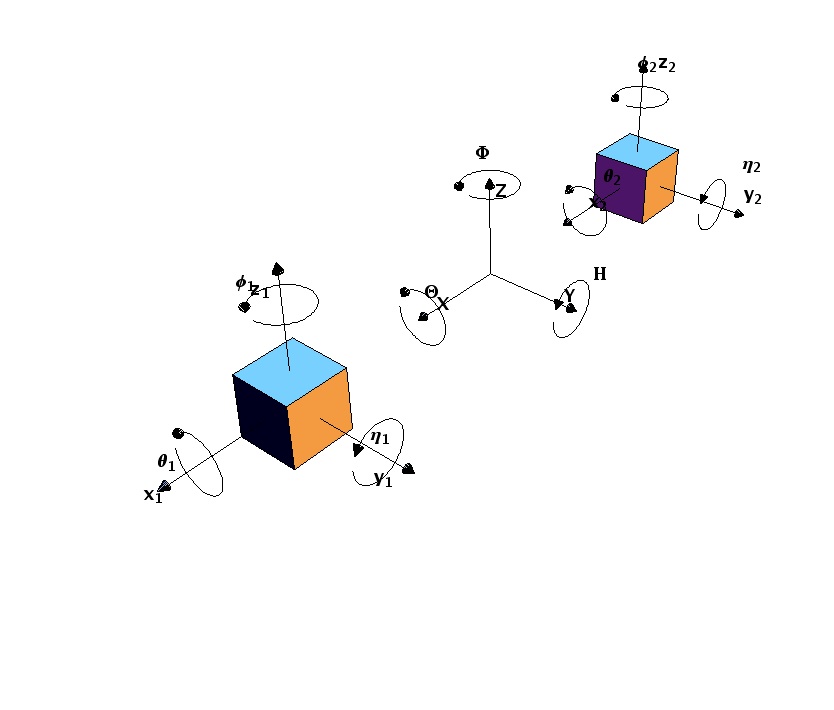
Figure 2.1: Fundamental reference systems on board LTP: TM1, TM2 and SC centre of mass coordinates are expressed as $6\times 3$ DOF, linear and conjugated angular.

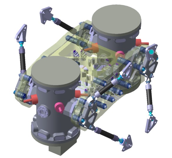
Figure 2.2: Rendering of external apparatus’s comprising Vacuum Enclosures (VE) of the Inertial Sensors (cylinders aside), Optical Bench (midway, semi-transparent), struts and fittings. The VE hold the Electrode Housings which in turn contain the TMs providing autonomous ultra high vacuum around the TMs (non visible). The optical bench in between the TMs (in grey) supports the interferometry that reads out the distance between the masses. The interferometer laser beam hits each TM by crossing the vacuum enclosures through an optical window. The entire supporting structure is made out of glass-ceramics for high therm mechanical stability. Optical fibres carrying UV light are used for contact less discharging of TMs.

The following reference frames may be considered:

1. $\text{SF}_{\text{CM}}$: the system of the SC centre of mass,

2. $\text{SF}_{\text{BF}}$: the body fixed reference frame of the SC,

3. $\text{ISF}i,\,i=1,2$: the body fixed reference frame of the IS electrode housing of TM1 and TM2 respectively.

In addition, a generic inertial frame IF may appear and in most cases all body fixed reference frames only differ for very small perturbations in displacement and rotations so that transformations of coordinates may be assumed as linear; Euler cross-terms will always be neglected in this spirit.

According to the mentioned frames, relevant systems of coordinates can be forged. The general dynamics - and hence all the signals - will be written as functions of these:

1. the TM-$i$ coordinates in the IF:

   $${\boldsymbol{x}}_{i}=\left[\begin{matrix}x\\ y\\ z\\ \theta\\ \eta\\ \phi\end{matrix}\right]_{i}\,,\,i=1,2\,,$$ (2.1)

   whose origins are taken to be the instantaneous positions of the nominal centres of the electrode housings; sometimes we may refer to the two translational and angular subsets of coordinates:

   $${\boldsymbol{x}}^{T}_{i}=\left[\begin{matrix}x\\ y\\ z\end{matrix}\right]_{i}\,,\qquad{\boldsymbol{x}}^{R}_{i}=\left[\begin{matrix}\theta\\ \eta\\ \phi\end{matrix}\right]_{i}\,.$$ (2.2)

   Notice ${\boldsymbol{x}}_{i}={\boldsymbol{x}}^{T}_{i}\leavevmode\nobreak\ \otimes\leavevmode\nobreak\ \left[\begin{matrix}1\\ 0\end{matrix}\right]+{\boldsymbol{x}}^{R}_{i}\leavevmode\nobreak\ \otimes\leavevmode\nobreak\ \left[\begin{matrix}0\\ 1\end{matrix}\right]$, for $i=1,2$.

2. The SC coordinates in the IF:

   $${\boldsymbol{X}}=\left[\begin{matrix}X\\ Y\\ Z\\ \Theta\\ H\\ \Phi\end{matrix}\right]\,,$$ (2.3)

   whose origin is the instantaneous position of the SC centre of mass.

3. The TMs coordinates in the ISF1 and 2:

   $${\boldsymbol{x}}^{\text{SC}}_{i}=\left[\begin{matrix}x\\ y\\ z\\ \theta\\ \eta\\ \phi\end{matrix}\right]^{\text{SC}}_{i}\,,\,i=1,2\,,$$ (2.4)

   origins are assumed in the nominal centres of the respective electrode housings. Their difference with the coordinates in the $SF_{\text{BF}}$ is a simple vector only if there’s no distortions at play. ${\boldsymbol{x}}^{\text{SC}}_{i}$ and ${\boldsymbol{x}}_{i}$ are related by a roto-translational transformation which will be clarified in the following.

4. The distortions of ISF1,2 relative to $SF_{\text{BF}}$:

   $${\boldsymbol{\delta x}}^{\text{SC}}_{i}=\left[\begin{matrix}\delta x\\ \delta y\\ \delta z\\ \delta\theta\\ \delta\eta\\ \delta\phi\end{matrix}\right]_{i}\,,$$ (2.5)

   which won’t be used extensively if not for sensitivity and cross-talk analysis.

Moreover, a caveat must be given at this time: TMs and SC are extended bodies, not point-like masses. Therefore, a complicated set of problems arise which are not present in the standard Newtonian approach for low velocity particles. Cross-talk summarises part of these, and carries dynamical, geometrical (affine) and electrostatics features: effective rotational arms between SC and TMs need to be taken into account, errors in positioning translating into rotational jitter, effective spring or magnetic couplings resulting from the extensiveness of the bodies. In section 3.5.7 we’ll deal with cross-talk in more detailed way.

Self-gravity acquires also multi-source features: the static imbalance of solid structures of the SC acts on the TMs in a very nontrivial way, not separable into a couple of point-like sources: relative stiffness and static gravity gradients demand a dedicated treatment and solution which we’ll tackle in section 4.2.

2.2 Signals

The generalised vectors ${\boldsymbol{x}}^{\text{SC}}_{i}$ are internal state vectors of LTP, while ${\boldsymbol{X}}$ is the state vector of the SC. Each TM is surrounded by electrodes (see figure 2.3) which can provide electrostatic readout of the position as well as induce motion by voltage actuation. From the state vectors we can generate signals encompassing noise in the definition:

$$\text{GRS}\left({\boldsymbol{x}}_{i}\right)={\boldsymbol{x}}_{i}^{\text{SC}}+\text{GRS}_{n}\left({\boldsymbol{x}}_{i}\right)\quad i=1,2\,,$$ (2.6)

where we defined the noise vectors $\text{GRS}_{n}\left({\boldsymbol{x}}_{i}\right)$, whose characteristic upper limits can be deduced from the capacitance sensors properties and, for the specific case of LTP are pointed out in table 2.1. Anywhere in the following, “GRS” designates the readout signal from the capacitance electronics and stands for Gravitational Reference Sensor.

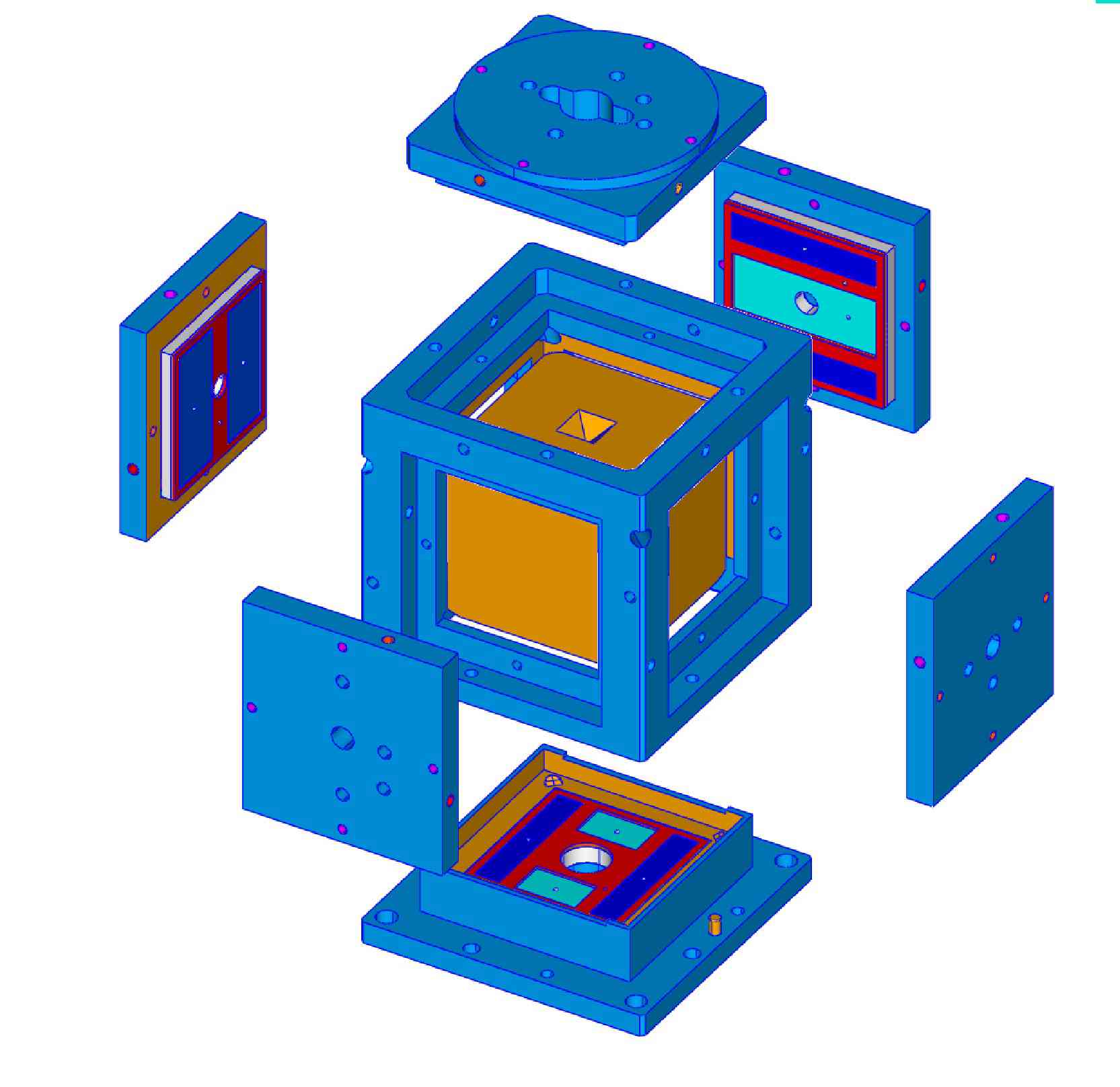
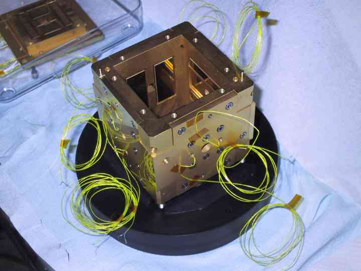
Figure 2.3: Top left: scheme of the LTP readout and actuation electrodes (GRS) per TM: GRS electrodes are held by the frame of the Electrode Housing and are characterised by many capacitance sleeves. The TM can be seen inside the frame structure. Top right: engineering model of housing on a table in the Low Temperature and Experimental Gravity Laboratory in Trento. GRS capacitors glitter inside the cube. Below: detail of electrodes per direction.

GRS disturbance	maximum at $1\,\mathrm{mHz}\leq f\leq 1\mathrm{Hz}$
$x^{n}_{i}$, $y^{n}_{i}$, $z^{n}_{i}$	$1.8\,\nicefrac{{\mathrm{nm}}}{{\mathrm{\sqrt{Hz}}}}$
$\phi^{n}_{i}$, $\eta^{n}_{i}$, $\theta^{n}_{i}$	$200\,\nicefrac{{\mathrm{nrad}}}{{\mathrm{\sqrt{Hz}}}}$

Table 2.1: Expected noise levels in GRS capacitive readout.

More sensitive than the electrostatic readout, a laser metrology equipment is placed aboard LTP in order to read 3 positions and 4 attitudes by means of quadrant photo-diodes. The ability of measurement with such a device is the core of the experiment, i.e. to detect the difference between the two $x^{\text{SC}}_{i}$ of the TMs. The signal vector is defined as:

$$\text{IFO}(\left[\begin{matrix}x_{1}\\ \phi_{1}\\ \eta_{1}\\ x_{2}\\ \phi_{2}\\ \eta_{2}\\ x_{2}-x_{1}\end{matrix}\right])=\left[\begin{matrix}x_{1}\\ \phi_{1}\\ \eta_{1}\\ x_{2}\\ \phi_{2}\\ \eta_{2}\\ x_{2}-x_{1}\end{matrix}\right]^{\text{SC}}+\text{IFO}_{n}(\left[\begin{matrix}x_{1}\\ \phi_{1}\\ \eta_{1}\\ x_{2}\\ \phi_{2}\\ \eta_{2}\\ x\end{matrix}\right])\,,$$ (2.7)

where we put the subscript $n$ to the laser noise. Laser sensitivity can be given as a power spectral density (PSD) function of frequency and can be viewed in figure 2.4. For attitude readout the photo-diode sensitivity on the angular signals and in frequency range $1\,\mathrm{mHz}\leq f\leq 1\,\mathrm{Hz}$ amounts to a maximum uncertainty of $10\,\nicefrac{{\mathrm{nrad}}}{{\mathrm{\sqrt{Hz}}}}$. The name “IFO” comes from InterFerometer Output.

Figure 2.4: Laser interferometer noise (lowest curve) as angular and linear displacement PSDs.

Last signals are originated by star-trackers, high-precision pointers directed to reference stars. These signals shall control rotational modes of the SC, which in principle wouldn’t be otherwise prevented to continuously rotate around the $\hat{x}$ sensing axis, wasting fuel and introducing more undesired couplings. Moreover, the solar panels of LTP must always be facing the Sun to maximise the power outcome [38], another reason to prevent LTP from spinning around $\hat{x}$. Therefore we define:

$$\text{ST}(\left[\begin{matrix}\Theta\\ H\\ \Phi\end{matrix}\right])=\left[\begin{matrix}\Theta\\ H\\ \Phi\end{matrix}\right]^{\text{SC}}+\text{ST}_{n}(\left[\begin{matrix}\Theta\\ H\\ \Phi\end{matrix}\right])\,,$$ (2.8)

whose angular PSD error for $f\leq 5\times 10^{-4}\,\mathrm{Hz}$ is $\leq 10^{-4}\,\nicefrac{{\mathrm{nrad}}}{{\mathrm{\sqrt{Hz}}}}$. These give reference attitude of the SC with respect to “fixed” stars and shall provide the needed control level.

2.3 Equations of motion

Given the coordinates systems and signals of the former section, a set of equations describing the unperturbed dynamics of LTP can be written. It is quite obvious that the kinetic matrix of the whole will be manifestly invariant with respect to any coupling we’d choose or any self-force. Besides, the form of the interaction terms and the couplings between signals and coordinates will change due to the control strategy we’d apply, other than the reference chosen.

For each TM and for the SC a set of generalised mass matrices can be defined:

$$M_{j}=\left[\begin{matrix}M_{j}^{T}&0\\ 0&M_{j}^{R}\end{matrix}\right]\,,$$ (2.9)

where $j=1,2,{\text{SC}}$ and the superscript $T,\,R$ in the sub-mass matrices define whether we are talking about a linear or angular DOF, to be multiplied by accelerations or velocities (linear or angular) in Newton or Lagrange equations. The $M_{j}^{R}$ are of course, principal moments of inertia matrices:

$$M_{j,ik}^{T}=m\delta_{ik}\,,\qquad M_{j,ik}^{R}=m\frac{L^{2}}{6}\delta_{ik}\,,$$ (2.10)

where $i,k=1..3$, $j=1,2$ and $\delta$ is the usual Kronecker delta indicator. We assumed perfect cubes with side length $L$ for the TMs shapes, having mass $m$. On the other hand, our picture of the SC is closer to a cylinder with height $\simeq$ radius $(R_{\text{SC}})$: the moments of inertia will be axis-wise different and we’ll get

$$M_{{\text{SC}},ik}^{T}=m_{\text{SC}}\delta_{ik}\,,\qquad M_{\text{SC}}^{R}=m_{\text{SC}}R^{2}_{\text{SC}}\left[\begin{matrix}\frac{1}{3}&0&0\\ 0&\frac{1}{3}&0\\ 0&0&\frac{1}{2}\end{matrix}\right]\,,$$ (2.11)

$m_{\text{SC}}$ being the SC mass. Stiffness matrices can be defined for both TMs, similarly:

$$K_{j}=\left[\begin{matrix}K_{j}^{T}&0\\ 0&K_{j}^{R}\end{matrix}\right]\,,$$ (2.12)

where

$$\begin{split}K_{j}^{T}&=m\left[\begin{matrix}\omega_{x_{j},x_{j}}^{2}&0&0\\ 0&\omega_{y_{j},y_{j}}^{2}&0\\ 0&0&\omega_{z_{j},z_{j}}^{2}\end{matrix}\right]\,,\\ K_{j}^{R}&=m\frac{L^{2}}{6}\left[\begin{matrix}\omega_{\theta_{j},\theta_{j}}^{2}&0&0\\ 0&\omega_{\eta_{j},\eta_{j}}^{2}&0\\ 0&0&\omega_{\phi_{j},\phi_{j}}^{2}\end{matrix}\right]\,,\end{split}$$ (2.13)

conversely, no need or opportunity to define similar matrices for the SC, which has no reference to be defined “dynamically stiff” to. In a word these matrices express the spring-like linear coupling of the TMs to the whole SC. Dimensions of the coefficients $\omega_{\hat{i},\hat{i}}^{2}$ is $\nicefrac{{1}}{{\mathrm{s^{2}}}}$.

External stimuli acting on each TM can be written as follows, along the linear and angular conjugated directions:

$$\begin{split}{\boldsymbol{F}}_{i}&=m\left[\begin{matrix}g_{x}\\ g_{y}\\ g_{z}\end{matrix}\right]_{i}\,,\\ {\boldsymbol{\gamma}}_{i}&=m\frac{L^{2}}{6}\left[\begin{matrix}g_{\theta}\\ g_{\eta}\\ g_{\phi}\end{matrix}\right]_{i}\,,\end{split}$$ (2.14)

while for the SC similar expressions hold, provided the following substitutions:

$$m\to m_{\text{SC}}\,,\qquad\frac{L^{2}}{6}\to R^{2}_{\text{SC}}\left[\begin{matrix}\frac{1}{3}&0&0\\ 0&\frac{1}{3}&0\\ 0&0&\frac{1}{2}\end{matrix}\right]\,.$$ (2.15)

From time to time we may be grouping forces and torques into generalised forces as ${\boldsymbol{f}}_{i}=F_{i}\leavevmode\nobreak\ \otimes\leavevmode\nobreak\ \left[\begin{array}[]{c}1\\ 0\end{array}\right]+\gamma_{i}\leavevmode\nobreak\ \otimes\leavevmode\nobreak\ \left[\begin{array}[]{c}0\\ 1\end{array}\right]$ and at even higher level we’ll define an indice-less ${\boldsymbol{f}}={\boldsymbol{f}}_{1}\leavevmode\nobreak\ \otimes\leavevmode\nobreak\ \left[\begin{array}[]{c}1\\ 0\end{array}\right]+{\boldsymbol{f}}_{2}\leavevmode\nobreak\ \otimes\leavevmode\nobreak\ \left[\begin{array}[]{c}0\\ 1\end{array}\right]$. The special vectors

$${\boldsymbol{r}}_{i}=\left[\begin{matrix}(-1)^{i}\frac{r_{0}}{2}\\ 0\\ z_{0}\end{matrix}\right]$$ (2.16)

define the unperturbed direction connecting the SC centre of mass to the TM-$i$ nominal positions. $r_{0}$ is the mutual distance between the two TMs and $z_{0}$ is the (vertical) distance between the TMs mutual $\hat{x}$ axis and the SC centre of mass.

The equations of motion in the TMs IF look then like:

$$M^{T}_{j}\ddot{{\boldsymbol{x}}}^{T}_{j}+K^{T}_{j}{\boldsymbol{x}}^{T}_{j} ={\boldsymbol{F}}_{j}\qquad j=1,2\,,$$ (2.17)

$$M^{R}_{j}\ddot{{\boldsymbol{x}}}^{R}_{j}+K^{R}_{j}{\boldsymbol{x}}^{R}_{j} ={\boldsymbol{\gamma}}_{j}\qquad j=1,2\,,$$ (2.18)

$$M^{T}_{\text{SC}}\ddot{{\boldsymbol{x}}}^{T}_{\text{SC}} ={\boldsymbol{F}}_{\text{SC}}\,,$$ (2.19)

$$M^{R}_{\text{SC}}\ddot{{\boldsymbol{x}}}^{R}_{\text{SC}} ={\boldsymbol{\gamma}}_{\text{SC}}\,,$$ (2.20)

and no sum is implied over repeated indice. As stated already, Euler self-coupling terms are and will be neglected in the following since they are small and can be dynamically compensated for by the actuation loops.

Since we want to keep track of things in the inertial frame of each TM, the SC motion must be taken into account. The relative change of coordinate in both translational and rotational frames can be accounted for with the transformation:

$$\begin{split}{\boldsymbol{F}}_{j}&\to{\boldsymbol{F}}_{j}-M^{T}_{j}\left(\ddot{{\boldsymbol{x}}}^{T}_{\text{SC}}+\ddot{{\boldsymbol{x}}}^{R}_{\text{SC}}\wedge{{\boldsymbol{r}}}_{j}\right)\,,\\ {\boldsymbol{\gamma}}_{j}&\to{\boldsymbol{\gamma}}_{j}-M^{R}_{j}\ddot{{\boldsymbol{x}}}^{R}_{\text{SC}}\,.\end{split}$$ (2.21)

Due to the wide application of control theory in Fourier and Laplace spaces to analyse the dynamics of the bodies, for most of the time we’ll write the equation in the frequency domain, i.e. we’ll make the association:

$$\dot{{\boldsymbol{x}}}\to s{\boldsymbol{x}}\,,\qquad s\doteq\imath\omega\,,$$ (2.22)

where $s(\omega)$ is the Laplace(Fourier) transformed time and we assume convergence in integration unless otherwise discussed. Our equations of motion are natively linear and being treated in Fourier space will lead us to deducing signals as “propagators” in the frequency domain. This is natural in control theory and permits a more transparent discussion on critical frequencies as well as measurement bandwidth and resonances. When discussing noise, we’ll make wide use of Power Spectral Densities (PSD), Fourier transforms of correlators, it seemed thus a wise choice to work in frequency space from here.

Expanding the unperturbed equations of motion from matrix to scalar form, we get the following set of coupled equations, $18$ in number; namely those for TM1:

$$mx_{1}s^{2}+m\left(x_{\text{SC}}+z_{0}\eta_{\text{SC}}\right)s^{2}+mx_{1}\omega_{x_{1},x_{1}}^{2}-mg_{1,x} =0\,,$$ (2.23)

$$my_{1}s^{2}+m\left(y_{\text{SC}}-z_{0}\theta_{\text{SC}}-\frac{r_{o}\phi_{\text{SC}}}{2}\right)s^{2}+my_{1}\omega_{y_{1},y_{1}}^{2}-mg_{1,y} =0\,,$$ (2.24)

$$mz_{1}s^{2}+m\left(z_{\text{SC}}+\frac{r_{o}\eta_{\text{SC}}}{2}\right)s^{2}+mz_{1}\omega_{z_{1},z_{1}}^{2}-mg_{1,z} =0\,,$$ (2.25)

$$\frac{1}{6}m\theta_{1}\omega_{\theta_{1},\theta_{1}}^{2}L^{2}+\frac{1}{6}ms^{2}\theta_{1}L^{2}+\frac{1}{6}ms^{2}\theta_{\text{SC}}L^{2}-\frac{1}{6}mg_{1,\theta}L^{2} =0\,,$$ (2.26)

$$\frac{1}{6}m\eta_{1}\omega_{\eta_{1},\eta_{1}}^{2}L^{2}+\frac{1}{6}ms^{2}\eta_{1}L^{2}+\frac{1}{6}ms^{2}\eta_{\text{SC}}L^{2}-\frac{1}{6}mg_{1,\eta}L^{2} =0\,,$$ (2.27)

$$\frac{1}{6}m\phi_{1}\omega_{\phi_{1},\phi_{1}}^{2}L^{2}+\frac{1}{6}ms^{2}\phi_{1}L^{2}+\frac{1}{6}ms^{2}\phi_{\text{SC}}L^{2}-\frac{1}{6}mg_{1,\phi}L^{2} =0\,,$$ (2.28)

those for TM2:

$$mx_{2}s^{2}+m\left(x_{\text{SC}}+z_{0}\eta_{\text{SC}}\right)s^{2}+mx_{2}\omega_{x_{2},x_{2}}^{2}-mg_{2,x} =0\,,$$ (2.29)

$$my_{2}s^{2}+m\left(y_{\text{SC}}-z_{0}\theta_{\text{SC}}+\frac{r_{o}\phi_{\text{SC}}}{2}\right)s^{2}+my_{2}\omega_{y_{2},y_{2}}^{2}-mg_{2,y} =0\,,$$ (2.30)

$$mz_{2}s^{2}+m\left(z_{\text{SC}}-\frac{r_{o}\eta_{\text{SC}}}{2}\right)s^{2}+mz_{2}\omega_{z_{2},z_{2}}^{2}-mg_{2,z} =0\,,$$ (2.31)

$$\frac{1}{6}m\theta_{2}\omega_{\theta_{2},\theta_{2}}^{2}L^{2}+\frac{1}{6}ms^{2}\theta_{2}L^{2}+\frac{1}{6}ms^{2}\theta_{\text{SC}}L^{2}-\frac{1}{6}mg_{2,\theta}L^{2} =0\,,$$ (2.32)

$$\frac{1}{6}m\eta_{2}\omega_{\eta_{2},\eta_{2}}^{2}L^{2}+\frac{1}{6}ms^{2}\eta_{2}L^{2}+\frac{1}{6}ms^{2}\eta_{\text{SC}}L^{2}-\frac{1}{6}mg_{2,\eta}L^{2} =0\,,$$ (2.33)

$$\frac{1}{6}m\phi_{2}\omega_{\phi_{2},\phi_{2}}^{2}L^{2}+\frac{1}{6}ms^{2}\phi_{2}L^{2}+\frac{1}{6}ms^{2}\phi_{\text{SC}}L^{2}-\frac{1}{6}mg_{2,\phi}L^{2} =0\,,$$ (2.34)

and those for the SC:

$$s^{2}m_{\text{SC}}x_{\text{SC}}-m_{\text{SC}}g_{\text{SC},x} =0\,,$$ (2.35)

$$s^{2}m_{\text{SC}}y_{\text{SC}}-m_{\text{SC}}g_{\text{SC},y} =0\,,$$ (2.36)

$$s^{2}m_{\text{SC}}z_{\text{SC}}-m_{\text{SC}}g_{\text{SC},z} =0\,,$$ (2.37)

$$\frac{1}{3}s^{2}m_{\text{SC}}R_{\text{SC}}^{2}\theta_{\text{SC}}-\frac{1}{3}m_{\text{SC}}R_{\text{SC}}^{2}g_{\text{SC},\theta} =0\,,$$ (2.38)

$$\frac{1}{3}s^{2}m_{\text{SC}}R_{\text{SC}}^{2}\eta_{\text{SC}}-\frac{1}{3}m_{\text{SC}}R_{\text{SC}}^{2}g_{\text{SC},\eta} =0\,,$$ (2.39)

$$\frac{1}{2}s^{2}m_{\text{SC}}R_{\text{SC}}^{2}\phi_{\text{SC}}-\frac{1}{2}m_{\text{SC}}R_{\text{SC}}^{2}g_{\text{SC},\phi} =0\,.$$ (2.40)

The true reduced dynamic is represented in terms of the TMs variables, the SC coordinates can be rid of by linear substitution into the equations, a process we’ll eventually get through after having elucidated something more about the signals.

2.4 Operation modes

The practical realisation and implementation of the control strategy give rise to what we call an operation mode [40, 41, 9]. The name comes from the fact that a certain strategy will be employed for TMs and SC control during a time-slice of the experiment, and sets of measures will be taken under those circumstances. Therefore the laws of motion in the specific situation will become a command mode for the space-probe. Each mode is thus qualified by three properties:

1. the mentioned control strategy, consisting in a set of feed-back laws,

2. the characteristic frequencies at play, together with actuation laws which will effectively provide signal to the controlling apparatus’s,

3. the gains, determining whether a control shall be called soft or hard, drag-free or suspension.

For each mode the former points will be carefully discussed, several approximation may come at hand and will be motivated.

A choice of principal signals must be made due to redundancy ($x_{1}$ can be measured by GRS or IFO, for example) in order to describe the dynamics and analyse the LTP frequency behaviour: a selection of signals can be extracted from the TMs DOF ${\boldsymbol{x}}=x_{1}\leavevmode\nobreak\ \otimes\leavevmode\nobreak\ \left[\begin{array}[]{c}1\\ 0\end{array}\right]+x_{2}\leavevmode\nobreak\ \otimes\leavevmode\nobreak\ \left[\begin{array}[]{c}0\\ 1\end{array}\right]$ with $\Omega\left({\boldsymbol{x}}\right)$ being the readout operator matrix in (2.41).

$$\Omega=\left[\begin{array}[]{cccccccccccc}\text{IFO}&0&0&0&0&0&0&0&0&0&0&0\\ 0&\text{GRS}&0&0&0&0&0&0&0&0&0&0\\ 0&0&\text{GRS}&0&0&0&0&0&0&0&0&0\\ 0&0&0&\text{GRS}&0&0&0&0&0&0&0&0\\ 0&0&0&0&\text{IFO}&0&0&0&0&0&0&0\\ 0&0&0&0&0&\text{IFO}&0&0&0&0&0&0\\ -\text{IFO}&0&0&0&0&0&\text{IFO}&0&0&0&0&0\\ 0&0&0&0&0&0&0&\text{GRS}&0&0&0&0\\ 0&0&0&0&0&0&0&0&\text{GRS}&0&0&0\\ 0&0&0&0&0&0&0&0&0&\text{GRS}&0&0\\ 0&0&0&0&-\text{IFO}&0&0&0&0&0&\text{IFO}&0\\ 0&0&0&0&0&-\text{IFO}&0&0&0&0&0&\text{IFO}\end{array}\right](\cdot)\,.$$ (2.41)

Notice this is a particularly wise choice of readout which maximises the use of interferometer signals. We point out that along the main “science” DOF redundancy of the signals is a key feature. Moreover, electrostatic force can be exerted on the TMs via the capacitance (GRS) system, while main readout in this scenario is IFO-based, thus reducing contamination. We get then a set of fundamental (and minimal) readout signals, whose expressions will look like:

$$\text{IFO}\left(x_{1}\right) =x_{1}+\text{IFO}_{n}\left(x_{1}\right)\,,$$ (2.42)

$$\text{GRS}\left(y_{1}\right) =y_{1}+\text{GRS}_{n}\left(y_{1}\right)\,,$$ (2.43)

$$\text{GRS}\left(z_{1}\right) =z_{1}+\text{GRS}_{n}\left(z_{1}\right)\,,$$ (2.44)

$$\text{GRS}\left(\theta_{1}\right) =\theta_{1}+\text{GRS}_{n}\left(\theta_{1}\right)\,,$$ (2.45)

$$\text{IFO}\left(\eta_{1}\right) =\eta_{1}+\text{IFO}_{n}\left(\eta_{1}\right)\,,$$ (2.46)

$$\text{IFO}\left(\phi_{1}\right) =\phi_{1}+\text{IFO}_{n}\left(\phi_{1}\right)\,,$$ (2.47)

$$\text{IFO}\left(x_{2}-x_{1}\right) =x_{2}-x_{1}+\text{IFO}_{n}\left(x_{2}-x_{1}\right)\,,$$ (2.48)

$$\text{GRS}\left(y_{2}\right) =y_{2}+\text{GRS}_{n}\left(y_{2}\right)\,,$$ (2.49)

$$\text{GRS}\left(z_{2}\right) =z_{2}+\text{GRS}_{n}\left(z_{2}\right)\,,$$ (2.50)

$$\text{GRS}\left(\theta_{2}\right) =\theta_{2}+\text{GRS}_{n}\left(\theta_{2}\right)\,,$$ (2.51)

$$\text{IFO}\left(\eta_{2}-\eta_{1}\right) =\eta_{2}-\eta_{1}+\text{IFO}_{n}\left(\eta_{2}-\eta_{1}\right)\,,$$ (2.52)

$$\text{IFO}\left(\phi_{2}-\phi_{1}\right) =\phi_{2}-\phi_{1}+\text{IFO}_{n}\left(\phi_{2}-\phi_{1}\right)\,.$$ (2.53)

The concept of feedback is then put at play. Drag-free is achieved by controlling the SC motion enslaved to TMs displacement, given some rules and a servo-control system. The most general expression we can write renders also transparent the full strategy: forces and torques acting on the SC are felt by Newton law as accelerations which jeopardise the inertiality of the TMs inside the LTP shielding. Such forces and torques are re-injected as additive terms of the general forces and torques acting on the TMs as functions of the SC displacement and attitude. Those terms can be seen as functions of the forces and torques acting on the SC. In formulae, we call control strategy the map:

$$\begin{split}{\boldsymbol{F}}_{j}&\to{\boldsymbol{F}}_{j}+{\boldsymbol{\hat{F}}}\left({\boldsymbol{x}}_{\text{SC}},\,\text{GRS}({\boldsymbol{x}}_{i}),\,\text{IFO}({\boldsymbol{x}}_{i}),\,\dots\right)\,,\\ {\boldsymbol{\gamma}}_{j}&\to{\boldsymbol{\gamma}}_{j}+{\boldsymbol{\hat{\gamma}}}\left({\boldsymbol{x}}_{\text{SC}},\,\text{GRS}({\boldsymbol{x}}_{i}),\,\text{IFO}({\boldsymbol{x}}_{i}),\,\dots\right)\,,\end{split}$$ (2.54)

where the dependence on the signals has been highlighted, meaning that control strategies will be essentially based on our knowledge of positions and therefore will naturally bring readout noise inside the equations.

2.4.1 Science mode

The main operating mode is christened “science mode”, formerly known as M3 [39]. (In the real mission, unless otherwise specified, in this mode the control loops are driven by signals obtained from inertial sensors capacitive readout (GRS) or interferometer. We chose here to maximise the use of IFO readout whenever possible). Both in the IFO MBW and below, the following control scheme is employed [26]:

• The SC is controlled in translation along $\hat{x}$ on TM1 This means that a force is applied to the SC by properly firing the thrusters:

  $$F^{\text{thrusters}}_{\text{SC},x}=m_{\text{SC}}\omega^{2}_{\text{df,x}}x_{1}\,,$$ (2.55)

• The gain $\omega^{2}_{\text{df,x}}$ must be representative of that of LISA in the entire control bandwidth $0\leq f\leq f_{0}$, with $f_{0}\geq 30\,\mathrm{mHz}$:

  $$m_{\text{SC}}\omega^{2}_{\text{df,x}}\geq 2\times 10^{2}\,\nicefrac{\mathrm{N}}{\mathrm{m}}\,.$$ (2.56)

• TM2 is subject to a low frequency suspension loop along $\hat{x}$ in order both to compensate for dc-forces and to stabilise its intrinsic negative stiffness. TM2 is controlled using the main laser channel so that it’s forced to follow TM1; the actuation force applied to TM2 by means of the capacitive system is:

  $$F^{\text{act}}_{2,x}=-m\omega^{2}_{\text{lfs},x}(x_{2}-x_{1})\,.$$ (2.57)

  The open-loop gain $m\omega^{2}_{\text{lfs},x}$ of the low frequency suspension (LFS, lfs in indice from now on) must guarantee that forces between DC and the lower end of the measuring bandwidth do not displace the TM by more than $1\,\mathrm{\mu m}$ from the nominal working point. The absolute value of the open-loop gain of the LFS within the MBW must be adjustable to be $\left|m\omega^{2}_{\text{lfs},x}\right|\leq 3\times 10^{-5}\,\nicefrac{\mathrm{N}}{\mathrm{m}}$ during calibration of the transfer function of the forces on TM to the IFO$(x_{2}-x_{1})$ signal: this way the gain is $\leq m\omega^{2}/2$ a the lowest corner of the MBW.

• The SC is controlled in translation along $\hat{y}$ on TM2 the same way as it is controlled on $\hat{x}$ for TM1.

• Similarly, the SC is controlled in translation along $\hat{z}$ on TM1.

• The SC is controlled in rotation around $\hat{z}$ and $\hat{y}$, within the MBW, by using the difference of the readouts of TM1 and TM2 along $\hat{y}$ and $\hat{z}$ respectively.

• TM1 and TM2 have no electrostatic suspension along $\hat{y}$ and $\hat{z}$ within the MBW.

• TM1 is subject to an electrostatic suspension along $\hat{y}$ below the MBW.

• TM2 is subject to an electrostatic suspension along $\hat{z}$ below the MBW.

• Rotation around $\hat{x}$, $\hat{y}$ and $\hat{z}$ below the MBW is controlled by star trackers.

• Rotation around $\hat{x}$ within the MBW is controlled on $\theta$ rotation of TM1.

• TM1 is subject to an electrostatic suspension for attitude control of $\hat{\phi}$ and $\hat{\eta}$.

• TM1 is subject to an electrostatic suspension for attitude control of $\hat{\theta}$ below the MBW.

• TM2 is subject to an electrostatic suspension for attitude control of $\hat{\phi}$, $\hat{\eta}$ and $\hat{\theta}$.

• The primary measurement goal is the PSD of the laser metrology output along $\hat{x}$, within the MBW.

The last statement is of course considered as the main mission goal. The aforementioned control-suspension strategy can be put at work by means of the signals we already defined, so that in the MBW we get the scheme as in table 2.2.

	$0\,\mathrm{mHz}\leq f\leq 0.5\,\mathrm{mHz}$		MBW, $0.5\,\mathrm{mHz}\leq f\leq 1\,\mathrm{Hz}$
State variable	Control signal	Gain	Control signal	Gain
$x_{1}$	-	$0$	-	$0$
$y_{1}$	GRS$(y_{1})$	$\omega_{\text{df},y}^{2}$	-	$0$
$z_{1}$	-	$0$	-	$0$
$\theta_{1}$	GRS$(\theta_{1})$	$\omega_{\text{df},\theta}^{2}$	-	$0$
$\eta_{1}$	IFO$(\eta_{1})$	$\omega_{\text{df},\eta}^{2}$	IFO$(\eta_{1})$	$\omega_{\text{lfs},\eta_{1}}^{2}$
$\phi_{1}$	IFO$(\phi_{1})$	$\omega_{\text{df},\phi}^{2}$	IFO$(\phi_{1})$	$\omega_{\text{lfs},\phi_{1}}^{2}$
$x_{2}$	IFO$(x_{2}-x_{1})$	$\omega_{\text{df},x}^{2}$	IFO$(x_{2}-x_{1})$	$\omega_{\text{lfs},x}^{2}$
$y_{2}$	-	$0$	-	$0$
$z_{2}$	GRS$(z_{2})$	$\omega_{\text{df},z}^{2}$	-	$0$
$\theta_{2}$	GRS$(\theta_{2})$	$\omega_{\text{df},\theta}^{2}$	GRS$(\theta_{2})$	$\omega_{\text{lfs},\theta}^{2}$
$\eta_{2}$	IFO$(\eta_{2})$	$\omega_{\text{df},\eta}^{2}$	IFO$(\eta_{2})$	$\omega_{\text{lfs},\eta_{2}}^{2}$
$\phi_{2}$	IFO$(\phi_{2})$	$\omega_{\text{df},\phi}^{2}$	IFO$(\phi_{2})$	$\omega_{\text{lfs},\phi_{2}}^{2}$
$X$	IFO$(x_{1})$	$\omega_{\text{df},x}^{2}$	IFO$(x_{1})$	$\omega_{\text{df},x}^{2}$
$Y$	GRS$(y_{2})$	$\omega_{\text{df},y}^{2}$	GRS$(y_{2})$	$\omega_{\text{df},y}^{2}$
$Z$	GRS$(z_{1})$	$\omega_{\text{df},z}^{2}$	GRS$(z_{1})$	$\omega_{\text{df},z}^{2}$
$\Theta$	ST$(\Theta)$	$\omega_{\text{df},\theta}^{2}$	IFO$(\theta_{1})$	$\omega_{\text{df},\theta}^{2}$
$H$	ST$(H)$	$\omega_{\text{df},\eta}^{2}$	GRS$(z_{2}-z_{1})$	$\omega_{\text{df},\eta}^{2}$
$\Phi$	ST$(\Phi)$	$\omega_{\text{df},\phi}^{2}$	GRS$(y_{2}-y_{1})$	$\omega_{\text{df},\phi}^{2}$

Table 2.2: Science (M3) mode: control logic and gain factors of suspensions and filters.

By inspecting the table we can see there’s two different regions in the frequency spectrum to be handled, the TMs are left as free as possible in the MBW, while ancillary DOF are “suspended” below it and overall the gain factors are tightened.

$$\Lambda_{1}=m \left[\begin{array}[]{cccccccccccc}0&0&0&0&0&0&0&0&0&0&0&0\\ 0&0&0&0&0&0&0&0&0&0&0&0\\ 0&0&0&0&0&0&0&0&0&0&0&0\\ 0&0&0&0&0&0&0&0&0&0&0&0\\ 0&0&0&0&\frac{1}{6}L^{2}\omega_{\text{lfs},\eta_{1}}^{2}&0&0&0&0&0&0&0\\ 0&0&0&0&0&\frac{1}{6}L^{2}\omega_{\text{lfs},\phi_{1}}^{2}&0&0&0&0&0&0\end{array}\right]\,$$ (2.64)

$$\Lambda_{2}=m \left[\begin{array}[]{cccccccccccc}0&0&0&0&0&0&\omega_{\text{lfs},x}^{2}&0&0&0&0&0\\ 0&0&0&0&0&0&0&0&0&0&0&0\\ 0&0&0&0&0&0&0&0&0&0&0&0\\ 0&0&0&0&0&0&0&0&0&\frac{1}{6}L^{2}\omega_{\text{lfs},\theta}^{2}&0&0\\ 0&0&0&0&0&0&0&0&0&0&\frac{1}{6}L^{2}\omega_{\text{lfs},\eta_{2}}^{2}&0\\ 0&0&0&0&0&0&0&0&0&0&0&\frac{1}{6}L^{2}\omega_{\text{lfs},\phi_{2}}^{2}\end{array}\right]\,,$$ (2.71)

$$\Lambda_{\text{SC}}=m_{\text{SC}} \left[\begin{array}[]{cccccccccccc}-\omega_{\text{df},x}^{2}&0&0&0&0&0&0&0&0&0&0&0\\ 0&-\omega_{\text{df},y}^{2}&0&0&0&0&0&0&0&0&0&0\\ 0&0&-\omega_{\text{df},z}^{2}&0&0&0&0&0&0&0&0&0\\ 0&0&0&-\frac{1}{3}R_{\text{SC}}^{2}\omega_{\text{df},\theta}^{2}&0&0&0&0&0&0&0&0\\ 0&0&-\frac{R_{\text{SC}}^{2}\omega_{\text{df},\eta}^{2}}{3r_{o}}&0&0&0&0&0&\frac{R_{\text{SC}}^{2}\omega_{\text{df},\eta}^{2}}{3r_{o}}&0&0&0\\ 0&\frac{R_{\text{SC}}^{2}\omega_{\text{df},\phi}^{2}}{2r_{o}}&0&0&0&0&0&-\frac{R_{\text{SC}}^{2}\omega_{\text{df},\phi}^{2}}{2r_{o}}&0&0&0&0\end{array}\right]\,.$$ (2.78)

Due to linearity, the feed-back action is obtained as the application of the counteraction matrices on the TMs coordinates ${\boldsymbol{x}}$, as follows:

$$\begin{split}\left[\begin{array}[]{c}{\boldsymbol{F}}_{j}\\ {\boldsymbol{\gamma}}_{j}\end{array}\right]&=-\Lambda_{j}\cdot{\boldsymbol{x}}\,,\qquad j=1,2\,,\\ \left[\begin{array}[]{c}{\boldsymbol{F}}_{\text{SC}}\\ {\boldsymbol{\gamma}}_{\text{SC}}\end{array}\right]&=-\Lambda_{\text{SC}}\cdot{\boldsymbol{x}}\,,\end{split}$$ (2.79)

where the form of the matrices is given in equations (2.64), (2.71) and (2.78). The resulting set of feed-back forces looks as follows, for TM1:

$$F_{1,x} =0\,,$$ (2.80)

$$F_{1,y} =0\,,$$ (2.81)

$$F_{1,z} =0\,,$$ (2.82)

$$\gamma_{1,\theta} =0$$ (2.83)

$$\gamma_{1,\eta} =-\frac{1}{6}L^{2}m\eta_{1}\omega_{\text{lfs},\eta_{1}}^{2}\,,$$ (2.84)

$$\gamma_{1,\phi} =-\frac{1}{6}L^{2}m\phi_{1}\omega_{\text{lfs},\phi_{1}}^{2}\,,$$ (2.85)

for TM2:

$$F_{2,x} =m\left(x_{1}-x_{2}\right)\omega_{\text{lfs},x}^{2}\,,$$ (2.86)

$$F_{2,y} =0\,,$$ (2.87)

$$F_{2,z} =0\,,$$ (2.88)

$$\gamma_{2,\theta} =-\frac{1}{6}L^{2}m\theta_{2}\omega_{\text{lfs},\theta}^{2}\,,$$ (2.89)

$$\gamma_{2,\eta} =-\frac{1}{6}L^{2}m\eta_{2}\omega_{\text{lfs},\eta_{2}}^{2}\,,$$ (2.90)

$$\gamma_{2,\phi} =-\frac{1}{6}L^{2}m\phi_{2}\omega_{\text{lfs},\phi_{2}}^{2}\,,$$ (2.91)

and finally for the SC:

$$F_{\text{SC},x} =m_{\text{SC}}x_{1}\omega_{\text{df},x}^{2}\,,$$ (2.92)

$$F_{\text{SC},y} =m_{\text{SC}}y_{1}\omega_{\text{df},y}^{2}\,,$$ (2.93)

$$F_{\text{SC},z} =m_{\text{SC}}z_{1}\omega_{\text{df},z}^{2}\,,$$ (2.94)

$$\gamma_{\text{SC},\theta} =\frac{1}{3}m_{\text{SC}}R_{\text{SC}}^{2}\theta_{1}\omega_{\text{df},\theta}^{2}\,,$$ (2.95)

$$\gamma_{\text{SC},\eta} =\frac{m_{\text{SC}}R_{\text{SC}}^{2}\left(z_{1}-z_{2}\right)\omega_{\text{df},\eta}^{2}}{3r_{o}}\,,$$ (2.96)

$$\gamma_{\text{SC},\phi} =\frac{m_{\text{SC}}R_{\text{SC}}^{2}\left(y_{2}-y_{1}\right)\omega_{\text{df},\phi}^{2}}{2r_{o}}\,.$$ (2.97)

A list of explanations is mandatory at this point:

1. the feed-back strategy is not unique. The main purpose of the set of counteractions at play in the $\Lambda_{j},\,j=1,2,\text{SC}$ is controlling the SC motion servo-ed to the TMs motions, leaving TM1 motion free along the $\hat{x}$ direction and interfering the least the better along the other directions.

2. The readout strategy is thought in this frame too: sensing along the $\hat{x}$ direction and anti-conjugated angular directions $\hat{\eta},\,\hat{\phi}$ is interferometer-based and electrostatic, with obvious noise-reduction-driven preferential choice of the first. Differential position between the TMs, differential angular and absolute position displacement of TM1 are thus IFO signals and considered as main mission signals. No DC force shall be applied in the $\hat{x},\,\hat{\eta},\,\hat{\phi}$ direction for TM1, and what is applicable in those directions for TM2 is strictly targeted to binding the TM2 motion to the SC.

3. Hidden in the symbols $\omega^{2}_{\text{lfs},i}$ and $\omega^{2}_{\text{df},i}$ we can retrieve then readout frequencies as well as control transfer functions, other than actuation filters. This strategy provides an enormous flexibility in assisting free-fall of TM1 by means of dragging the satellite apart, the reverse side of the medal is nevertheless twofold:

   noise

   coming out of measurement and actuation devices mix, complicating our model,

   actuation

   requires fine-tuning and orthogonalization to reduce cross-talk and optimisation of the effect: part of this process is dynamical and cannot be simply designed on-ground. Stiffness measurement strategies must be accounted for.

In view of a careful analysis of cross-talk and to group the results till now for the readers trained in control-theory, the overall dynamics can then be thought of as follows:

$$\begin{split}\left(Ms^{2}-K\right)\cdot{\boldsymbol{x}}+s^{2}J{\boldsymbol{x}}_{\text{SC}}=-\Lambda\cdot{\boldsymbol{x}}\,,\\ M_{\text{SC}}s^{2}{\boldsymbol{x}}_{\text{SC}}=-\Lambda_{\text{SC}}{\boldsymbol{x}}\,,\end{split}$$ (2.98)

where we tensor-grouped the whole kinetic, stiffness, control and readout matrices for the TMs as:

$$\begin{split}M&=\left[\begin{array}[]{cc}M_{1}&0\\ 0&M_{2}\end{array}\right]\,,\qquad K=\left[\begin{array}[]{cc}K_{1}&0\\ 0&K_{2}\end{array}\right]\,,\\ \Lambda&=\Lambda_{1}\leavevmode\nobreak\ \otimes\leavevmode\nobreak\ \left[\begin{array}[]{c}1\\ 0\end{array}\right]+\Lambda_{2}\leavevmode\nobreak\ \otimes\leavevmode\nobreak\ \left[\begin{array}[]{c}0\\ 1\end{array}\right]\,.\end{split}$$ (2.99)

And $J$ is a matrix containing torsion arms coefficients to embody the change of reference in expression (2.21). The second of (2.98) can be solved in ${\boldsymbol{x}}_{\text{SC}}$ to give:

$${\boldsymbol{x}}_{\text{SC}}=-\frac{1}{s^{2}}M_{\text{SC}}^{-1}\Lambda_{\text{SC}}{\boldsymbol{x}}$$ (2.100)

and back-substituted into (2.98) to get rid of the SC variables as follows:

$$\left(Ms^{2}-K\right){\boldsymbol{x}}=\left(-\Lambda+JM_{\text{SC}}^{-1}\Lambda_{\text{SC}}\right){\boldsymbol{x}}\doteq\hat{\Lambda}{\boldsymbol{x}}\,.$$ (2.101)

We now process all equations with the $\Omega(\cdot)$ operator, which has the effect to switch from deterministic variables to signals, introducing the readout strategy and the proper noise coupled to each detector.

At the end of the process, we are left with the following set of coupled linear equations:

$$\frac{m\text{GRS}\left(z_{1}\right)z_{0}\omega_{\text{df},\eta}^{2}}{r_{o}}-\frac{m\text{GRS}\left(z_{2}\right)z_{0}\omega_{\text{df},\eta}^{2}}{r_{o}}+m\text{IFO}\left(x_{1}\right)\left(s^{2}+\omega_{\text{df},x}^{2}+\omega_{x_{1},x_{1}}^{2}\right)=m\left(g_{1,x}-g_{\text{SC},x}-z_{0}g_{\text{SC},\eta}\right)+m\left(s^{2}+\omega_{x_{1},x_{1}}^{2}\right)\text{IFO}_{n}\left(x_{1}\right) \,,$$ (2.102)

$$-m\text{GRS}\left(\theta_{1}\right)z_{0}\omega_{\text{df},\theta}^{2}-\frac{1}{2}m\text{GRS}\left(y_{2}\right)\omega_{\text{df},\phi}^{2}+\frac{1}{2}m\text{GRS}\left(y_{1}\right)\left(2\omega_{\text{df},y}^{2}+\omega_{\text{df},\phi}^{2}+2\left(s^{2}+\omega_{y_{1},y_{1}}^{2}\right)\right)=\qquad$$

$$\frac{1}{2}m\left(2g_{1,y}-2g_{\text{SC},y}+2z_{0}g_{\text{SC},\theta}+r_{o}g_{\text{SC},\phi}\right)+m\left(s^{2}+\omega_{y_{1},y_{1}}^{2}\right)\text{GRS}_{n}\left(y_{1}\right) \,,$$ (2.103)

$$\frac{1}{2}m\text{GRS}\left(z_{1}\right)\left(2\omega_{\text{df},z}^{2}+\omega_{\text{df},\eta}^{2}+2\left(s^{2}+\omega_{z_{1},z_{1}}^{2}\right)\right)-\frac{1}{2}m\text{GRS}\left(z_{2}\right)\omega_{\text{df},\eta}^{2}=mg_{1,z}-\frac{1}{2}m\left(2g_{\text{SC},z}+r_{o}g_{\text{SC},\eta}\right)+m\left(s^{2}+\omega_{z_{1},z_{1}}^{2}\right)\text{GRS}_{n}\left(z_{1}\right) \,,$$ (2.104)

$$\frac{1}{6}L^{2}m\text{GRS}\left(\theta_{1}\right)\left(s^{2}+\omega_{\text{df},\theta}^{2}+\omega_{\theta_{1},\theta_{1}}^{2}\right)=\frac{1}{6}m\left(g_{1,\theta}-g_{\text{SC},\theta}\right)L^{2}+\frac{1}{6}m\left(s^{2}+\omega_{\theta_{1},\theta_{1}}^{2}\right)\text{GRS}_{n}\left(\theta_{1}\right)L^{2} \,,$$ (2.105)

$$\frac{m\text{GRS}\left(z_{1}\right)\omega_{\text{df},\eta}^{2}L^{2}}{6r_{o}}-\frac{m\text{GRS}\left(z_{2}\right)\omega_{\text{df},\eta}^{2}L^{2}}{6r_{o}}+\frac{1}{6}m\text{IFO}\left(\eta_{1}\right)\left(s^{2}+\omega_{\text{lfs},\eta_{1}}^{2}+\omega_{\eta_{1},\eta_{1}}^{2}\right)L^{2}=\frac{1}{6}m\left(g_{1,\eta}-g_{\text{SC},\eta}\right)L^{2}+\frac{1}{6}m\left(s^{2}+\omega_{\eta_{1},\eta_{1}}^{2}\right)\text{IFO}_{n}\left(\eta_{1}\right)L^{2} \,,$$ (2.106)

$$-\frac{m\text{GRS}\left(y_{1}\right)\omega_{\text{df},\phi}^{2}L^{2}}{6r_{o}}+\frac{m\text{GRS}\left(y_{2}\right)\omega_{\text{df},\phi}^{2}L^{2}}{6r_{o}}+\frac{1}{6}m\text{IFO}\left(\phi_{1}\right)\left(s^{2}+\omega_{\text{lfs},\phi_{1}}^{2}+\omega_{\phi_{1},\phi_{1}}^{2}\right)L^{2}=\frac{1}{6}m\left(g_{1,\phi}-g_{\text{SC},\phi}\right)L^{2}+\frac{1}{6}m\left(s^{2}+\omega_{\phi_{1},\phi_{1}}^{2}\right)\text{IFO}_{n}\left(\phi_{1}\right)L^{2} \,,$$ (2.107)

$$\frac{m\text{GRS}\left(z_{1}\right)z_{0}\omega_{\text{df},\eta}^{2}}{r_{o}}-\frac{m\text{GRS}\left(z_{2}\right)z_{0}\omega_{\text{df},\eta}^{2}}{r_{o}}+m\text{IFO}\left(x_{1}\right)\left(s^{2}+\omega_{\text{df},x}^{2}+\omega_{x_{2},x_{2}}^{2}\right)+m\text{IFO}\left(x_{2}-x_{1}\right)\left(s^{2}+\omega_{\text{lfs},x}^{2}+\omega_{x_{2},x_{2}}^{2}\right)=\qquad$$

$$m\left(g_{2,x}-g_{\text{SC},x}-z_{0}g_{\text{SC},\eta}\right)+m\left(s^{2}+\omega_{x_{2},x_{2}}^{2}\right)\text{IFO}_{n}\left(x_{1}\right)+m\left(s^{2}+\omega_{x_{2},x_{2}}^{2}\right)\text{IFO}_{n}\left(x_{2}-x_{1}\right) \,,$$ (2.108)

$$-m\text{GRS}\left(\theta_{1}\right)z_{0}\omega_{\text{df},\theta}^{2}+\text{GRS}\left(y_{1}\right)\left(m\omega_{\text{df},y}^{2}-\frac{1}{2}m\omega_{\text{df},\phi}^{2}\right)+\frac{1}{2}m\text{GRS}\left(y_{2}\right)\left(\omega_{\text{df},\phi}^{2}+2\left(s^{2}+\omega_{y_{2},y_{2}}^{2}\right)\right)=\qquad$$

$$mg_{2,y}-mg_{\text{SC},y}+mz_{0}g_{\text{SC},\theta}-\frac{1}{2}mr_{o}g_{\text{SC},\phi}+m\left(s^{2}+\omega_{y_{2},y_{2}}^{2}\right)\text{GRS}_{n}\left(y_{2}\right) \,,$$ (2.109)

$$\text{GRS}\left(z_{1}\right)\left(m\omega_{\text{df},z}^{2}-\frac{1}{2}m\omega_{\text{df},\eta}^{2}\right)+\frac{1}{2}m\text{GRS}\left(z_{2}\right)\left(\omega_{\text{df},\eta}^{2}+2\left(s^{2}+\omega_{z_{2},z_{2}}^{2}\right)\right)=\frac{1}{2}m\left(2g_{2,z}-2g_{\text{SC},z}+r_{o}g_{\text{SC},\eta}\right)+m\left(s^{2}+\omega_{z_{2},z_{2}}^{2}\right)\text{GRS}_{n}\left(z_{2}\right) \,,$$ (2.110)

$$\frac{1}{6}m\text{GRS}\left(\theta_{1}\right)\omega_{\text{df},\theta}^{2}L^{2}+\frac{1}{6}m\text{GRS}\left(\theta_{2}\right)\left(s^{2}+\omega_{\text{lfs},\theta}^{2}+\omega_{\theta_{2},\theta_{2}}^{2}\right)L^{2}=\frac{1}{6}m\left(g_{2,\theta}-g_{\text{SC},\theta}\right)L^{2}+\frac{1}{6}m\left(s^{2}+\omega_{\theta_{2},\theta_{2}}^{2}\right)\text{GRS}_{n}\left(\theta_{2}\right)L^{2} \,,$$ (2.111)

$$\frac{m\text{GRS}\left(z_{1}\right)\omega_{\text{df},\eta}^{2}L^{2}}{6r_{o}}-\frac{m\text{GRS}\left(z_{2}\right)\omega_{\text{df},\eta}^{2}L^{2}}{6r_{o}}+\frac{1}{6}m\text{IFO}\left(\eta_{1}\right)\left(s^{2}+\omega_{\text{lfs},\eta_{2}}^{2}+\omega_{\eta_{2},\eta_{2}}^{2}\right)L^{2}+\frac{1}{6}m\text{IFO}\left(\eta_{2}-\eta_{1}\right)\left(s^{2}+\omega_{\text{lfs},\eta_{2}}^{2}+\omega_{\eta_{2},\eta_{2}}^{2}\right)L^{2}=\qquad$$

$$\frac{1}{6}m\left(g_{2,\eta}-g_{\text{SC},\eta}\right)L^{2}+\frac{1}{6}m\left(s^{2}+\omega_{\eta_{2},\eta_{2}}^{2}\right)\text{IFO}_{n}\left(\eta_{1}\right)L^{2}\frac{1}{6}m\left(s^{2}+\omega_{\eta_{2},\eta_{2}}^{2}\right)\text{IFO}_{n}\left(\eta_{2}-\eta_{1}\right)L^{2} \,,$$ (2.112)

$$-\frac{m\text{GRS}\left(y_{1}\right)\omega_{\text{df},\phi}^{2}L^{2}}{6r_{o}}+\frac{m\text{GRS}\left(y_{2}\right)\omega_{\text{df},\phi}^{2}L^{2}}{6r_{o}}+\frac{1}{6}m\text{IFO}\left(\phi_{1}\right)\left(s^{2}+\omega_{\text{lfs},\phi_{2}}^{2}+\omega_{\phi_{2},\phi_{2}}^{2}\right)L^{2}+\frac{1}{6}m\text{IFO}\left(\phi_{2}-\phi_{1}\right)\left(s^{2}+\omega_{\text{lfs},\phi_{2}}^{2}+\omega_{\phi_{2},\phi_{2}}^{2}\right)L^{2}=\qquad$$

$$\frac{1}{6}m\left(g_{2,\phi}-g_{\text{SC},\phi}\right)L^{2}+\frac{1}{6}m\left(s^{2}+\omega_{\phi_{2},\phi_{2}}^{2}\right)\text{IFO}_{n}\left(\phi_{1}\right)L^{2}+\frac{1}{6}m\left(s^{2}+\omega_{\phi_{2},\phi_{2}}^{2}\right)\text{IFO}_{n}\left(\phi_{2}-\phi_{1}\right)L^{2} \,.$$ (2.113)

After diagonalising we can express the signals explicitly; not to harass on the reader we decided to write down only the IFO signals and the GRS signals will be displayed at need only; here, IFO$(\Delta x)$:

$$\begin{split}\text{IFO}&\left(x_{2}-x_{1}\right)=h_{x,x_{2},x_{2}}^{\text{lfs}}(\omega)h_{1}(\omega)h_{x,x_{1},x_{1}}(\omega)\\ &\Bigl{(}-\frac{\omega_{\text{df},x}^{2}\left(\omega_{x_{1},x_{1}}^{2}-\omega_{x_{2},x_{2}}^{2}\right)}{h_{1}(\omega)}\text{IFO}_{n}\left(x_{1}\right)-\frac{2z_{0}\omega_{\text{df},\eta}^{2}\left(\omega_{x_{1},x_{1}}^{2}-\omega_{x_{2},x_{2}}^{2}\right)}{r_{0}h_{0,z_{1},z_{1}}(\omega)h_{z,z_{2},z_{2}}(\omega)}\text{GRS}_{n}\left(z_{1}\right)\\ &+\frac{1}{h_{1}(\omega)h_{0,x_{2},x_{2}}(\omega)h_{x,x_{1},x_{1}}(\omega)}\text{IFO}_{n}\left(x_{2}-x_{1}\right)+\frac{2z_{0}\omega_{\text{df},\eta}^{2}\left(\omega_{x_{1},x_{1}}^{2}-\omega_{x_{2},x_{2}}^{2}\right)}{r_{0}h_{0,z_{2},z_{2}}(\omega)h_{z,z_{1},z_{1}}(\omega)}\text{GRS}_{n}\left(z_{2}\right)\\ &-\frac{1}{h_{1}(\omega)h_{x,x_{2},x_{2}}(\omega)}g_{1,x}-\frac{2z_{0}\omega_{\text{df},\eta}^{2}\left(\omega_{x_{1},x_{1}}^{2}-\omega_{x_{2},x_{2}}^{2}\right)}{r_{0}h_{z,z_{2},z_{2}}(\omega)}g_{1,z}+\frac{1}{h_{1}(\omega)h_{x,x_{1},x_{1}}(\omega)}g_{2,x}+\frac{2z_{0}\omega_{\text{df},\eta}^{2}\left(\omega_{x_{1},x_{1}}^{2}-\omega_{x_{2},x_{2}}^{2}\right)}{r_{0}h_{z,z_{1},z_{1}}(\omega)}g_{2,z}\\ &-\frac{\omega_{x_{1},x_{1}}^{2}-\omega_{x_{2},x_{2}}^{2}}{h_{1}(\omega)}g_{\text{SC},x}-\frac{2z_{0}\omega_{\text{df},\eta}^{2}\left(\omega_{x_{1},x_{1}}^{2}-\omega_{x_{2},x_{2}}^{2}\right)\left(\omega_{z_{1},z_{1}}^{2}-\omega_{z_{2},z_{2}}^{2}\right)}{r_{0}}g_{\text{SC},z}-\frac{2z_{0}\left(\omega_{x_{1},x_{1}}^{2}-\omega_{x_{2},x_{2}}^{2}\right)}{h_{0,z_{2},z_{2}}(\omega)h_{z,z_{1},z_{1}}(\omega)}g_{\text{SC},\eta}\Bigr{)}\,,\end{split}$$ (2.114)

where

$$\frac{1}{h_{1}(\omega)} =\frac{2\omega_{\text{df},z}^{2}}{h_{\eta,z_{2},z_{2}}(\omega)}+\omega_{\text{df},\eta}^{2}\left(\frac{1}{h_{0,z_{2},z_{2}}(\omega)}+\frac{1}{h_{0,z_{1},z_{1}}(\omega)}\right)+\frac{2}{h_{0,z_{1},z_{1}}(\omega)h_{0,z_{2},z_{2}}(\omega)}\,,$$ (2.115)

$$\frac{1}{h_{2}(\omega)} =\frac{2\omega_{\text{df},y}^{2}}{h_{\phi,y_{2},y_{2}}(\omega)}+\omega_{\text{df},\phi}^{2}\left(\frac{1}{h_{0,y_{2},y_{2}}(\omega)}+\frac{1}{h_{0,y_{1},y_{1}}(\omega)}\right)+\frac{2}{h_{0,y_{1},y_{1}}(\omega)h_{0,y_{2},y_{2}}(\omega)}\,,$$ (2.116)

and the general form of the filter functions $h$ can be written down as:

$$h_{x_{\hat{i}},x_{\hat{j}},x_{\hat{k}}}(\omega)=\frac{1}{\omega_{\text{df},x_{\hat{i}}}^{2}+\omega^{2}_{x_{\hat{j}},x_{\hat{k}}}-\omega^{2}}\,,$$ (2.117)

meaning the function is characterised by a drag-free high-gain transfer function, namely $\omega_{\text{df},x_{\hat{i}}}^{2}$, along the $\hat{i}$-th DOF, but also coupled to other axes or angular variables by means of a correction $\omega^{2}_{x_{\hat{j}},x_{\hat{k}}}$ which doesn’t necessarily need to be small at this level. In this chapter we’ll consider only diagonal couplings, so that $\hat{j}\equiv\hat{k}$, but we leave the set of symbols open for a more careful discussion about cross-talk, to be placed in the noise and disturbances chapter.

LFS functions will take the form:

$$h^{\text{lfs}}_{x_{\hat{i}},x_{\hat{j}},x_{\hat{k}}}(\omega)=\frac{1}{\omega_{\text{lfs},x_{\hat{i}}}^{2}+\omega^{2}_{x_{\hat{j}},x_{\hat{k}}}-\omega^{2}}\,,$$ (2.118)

differing from the drag-free ones in the values of the LFS transfer filters. We used a sloppier notation for the special cases when constants happen to be null, in absence of suspension or control, namely:

$$h_{x_{\hat{i}},x_{\hat{j}},x_{\hat{k}}}(\omega)\underset{\omega_{\text{df},x_{\hat{i}}}^{2}\to 0}{\to}h_{0,x_{\hat{j}},x_{\hat{k}}}(\omega)\equiv h^{\text{lfs}}_{0,x_{\hat{j}},x_{\hat{k}}}(\omega)\,,$$ (2.119)

more limiting cases occur when the additional couplings can be neglected or considered small enough to be perturbations, so that all filters collapse into drag-free parametrised families:

$$h_{x_{\hat{i}},x_{\hat{j}},x_{\hat{k}}}(\omega)\underset{\omega^{2}_{x_{\hat{j}},x_{\hat{k}}}\to 0}{\to}h_{x_{\hat{i}}}(\omega)\doteq\frac{1}{\omega_{\text{df},x_{\hat{i}}}^{2}-\omega^{2}}\,,$$ (2.120)

and obviously perturbations can be analysed to first order at need around these former considered as “zeroes”:

$$h_{x_{\hat{i}},x_{\hat{j}},x_{\hat{k}}}(\omega)\underset{\omega^{2}_{x_{\hat{j}},x_{\hat{k}}}\ll 1}{\simeq}h_{x_{\hat{i}}}(\omega)\left(1-h_{x_{\hat{i}}}(\omega)\omega^{2}_{x_{\hat{j}},x_{\hat{k}}}\right)\,.$$ (2.121)

These approximations can be put at play to inspect the signal formulae and cast a deeper glance to the arguments leading to the choice of operation modes. To leading order, in absence of any noise and any additional coupling apart from the LFS, we can write for the main signal as:

$$\text{IFO}\left(x_{2}-x_{1}\right)\simeq\frac{g_{2,x}-g_{1,x}}{\omega_{\text{lfs},x}^{2}-\omega^{2}}\,,$$ (2.122)

i.e. as aforementioned, the main mission interferometric signal represents a readout on the relative acceleration of the TMs, properly scaled to the modulation functions cast by the control and laser devices. We can study the main science signal more carefully, in the limit when the parasitic stiffness $\omega^{2}_{\text{p},1}\equiv\omega^{2}_{x_{1},x_{1}}$ and $\omega^{2}_{\text{p},2}\equiv\omega^{2}_{x_{2},x_{2}}$ are small compared to $\omega^{2}_{\text{df},x}$ and to leading order in $\nicefrac{{\omega^{2}_{\text{df},x}}}{{\omega^{2}}}$ within the MBW, to get:

$$\begin{split}\text{IFO}\left(x_{2}-x_{1}\right)\simeq\frac{1}{\omega_{\text{lfs},x}^{2}-\omega^{2}}\Bigl{(}&g_{2,x}-g_{1,x}-\text{IFO}_{n}(x_{1})\omega^{2}+(\delta x_{2}-\delta x_{1})\omega_{\text{p},2}^{2}+\\ &+\left(\omega_{\text{p},2}^{2}-\omega_{\text{p},1}^{2}\right)\left(\text{IFO}_{n}(x_{1})+\frac{g_{\text{SC},x}+z_{0}g_{\text{SC},\eta}}{\omega^{2}_{\text{df},x}}\right)\Bigr{)}\,.\end{split}$$ (2.123)

This fundamental formula has been recast in this shape for its paramount importance. It will be employed widely on discussing the noise contributions and apportioning and it’s the most reliable laser phase estimator we have: in the spirit of chapter 1 this signal describes our real ability to measure differential accelerations and thus to build a TT-gauged frame of reference. The deformation contribution $(\delta x_{2}-\delta x_{1})\omega_{\text{p},2}^{2}$ has been placed in (2.123) by hand, the presence of all deformations in the analytical deduction of the dynamical model would have engorged the formulae lessening the already nightmarish legibility.

In absence of external forces ($g_{\text{SC},x}+z_{0}g_{\text{SC},\eta}=0$) the signal is in fact representative of the acceleration noise provided the dynamical contribution of deformation is negligible with respect to the readout noise:

$$\left|{\delta}x_{2}-{\delta}x_{1}\right|\ll\text{IFO}_{n}(x_{1})\,,$$ (2.124)

besides, laser noise contribution to (2.123) is a very small fraction of the noise budget.

The interferometer signal on the $x_{1}$ DOF looks like:

$$\begin{split}\text{IFO}\left(x_{1}\right)\simeq&\frac{1}{\left(\omega^{2}-\omega_{\text{df},x}^{2}\right)\left(\omega^{2}-\omega_{\text{df},\eta}^{2}\right)}\\ &\Bigl{(}-\frac{z_{0}g_{1,z}\omega_{\text{df},\eta}^{2}}{r_{0}}+\frac{z_{0}g_{2,z}\omega_{\text{df},\eta}^{2}}{r_{0}}+g_{1,x}\left(\omega_{\text{df},\eta}^{2}-\omega^{2}\right)+\\ &+z_{0}g_{\text{SC},\eta}\omega^{2}+g_{\text{SC},x}\left(\omega^{2}-\omega_{\text{df},\eta}^{2}\right)\\ &+\omega^{2}\left(\omega^{2}-\omega_{\text{df},\eta}^{2}\right)\text{IFO}_{n}\left(x_{1}\right)+\frac{\omega^{2}z_{0}\omega_{\text{df},\eta}^{2}}{r_{0}}\left(\text{GRS}_{n}\left(z_{1}\right)-\text{GRS}_{n}\left(z_{2}\right)\right)\Bigr{)}=\\ \simeq&\frac{1}{\omega^{2}_{\text{df},x}}\Bigl{(}-\frac{z_{0}g_{1,z}}{r_{0}}+\frac{z_{0}g_{2,z}}{r_{0}}+g_{1,x}-g_{\text{SC},x}\\ &+\left(\omega_{\text{p},1}^{2}-\omega^{2}\right)\left(\text{IFO}_{n}(x_{1})-\delta x_{1}\right)\Bigr{)}=\\ \simeq&\frac{g_{\text{SC},x}}{\omega^{2}_{\text{df},x}}\,,\end{split}$$ (2.125)

where the already mentioned approximations have been used in cascade. The last passage emerges taking $\omega^{2}_{\text{df},x}$ to leading order and assuming the forces acting on the SC along $\hat{x}$ to be dominant. Analogously we get for $z_{1}$:

$$\begin{split}\text{GRS}\left(z_{1}\right)\simeq&\frac{1}{\omega_{\text{df},\eta}^{2}}\left(\frac{g_{1,z}}{2}-\frac{g_{2,z}}{2}-\frac{r_{0}g_{\text{SC},\eta}}{2}\right)-\frac{1}{\omega^{2}}\left(\frac{g_{1,z}}{2}+\frac{g_{2,z}}{2}-g_{\text{SC},z}\right)\\ &+\frac{1}{2}\text{GRS}_{n}\left(z_{1}\right)+\frac{1}{2}\text{GRS}_{n}\left(z_{2}\right)\,,\end{split}$$ (2.126)

and for $\theta_{1}$:

$$\text{GRS}\left(\theta_{1}\right)\simeq\frac{1}{\omega_{\text{df$\theta$}}^{2}}\left(g_{1,\theta}-g_{\text{SC},\theta}-\omega^{2}\text{GRS}_{n}\left(\theta_{1}\right)\right)\,,$$ (2.127)

and finally for $\phi_{1}$:

$$\begin{split}\text{IFO}\left(\phi_{1}\right)\simeq&\frac{1}{r_{0}\omega_{\text{df},\phi}^{2}}\left(g_{2,y}-g_{1,y}-r_{0}g_{\text{SC},\phi}\right)+\frac{1}{r_{0}\omega^{2}}\left(g_{2,y}-g_{1,y}-r_{0}g_{1,\phi}\right)\\ &+\frac{1}{r_{0}}\left(\text{GRS}_{n}\left(y_{1}\right)-\text{GRS}_{n}\left(y_{2}\right)\right)+\text{IFO}_{n}\left(\phi_{1}\right)\,.\end{split}$$ (2.128)

These signals are good estimators of noise and main signals contributions and can be very powerful when used together. For example (2.125) together with:

$$\text{GRS}(x_{2})\simeq\text{GRS}_{n}(x_{2})-\text{GRS}_{n}(x_{1})-\frac{g_{\text{SC},x}}{\omega^{2}_{\text{df},x}}+\text{IFO}_{n}(x_{2}-x_{1})\frac{\omega^{2}_{\text{lfs},x}}{\omega^{2}_{\text{lfs},x}-\omega^{2}}\,,$$ (2.129)

and

$$\text{GRS}(x_{1})\simeq-\frac{g_{\text{SC},x}}{\omega^{2}_{\text{df},x}}-\text{GRS}_{n}(x_{1})\,,$$ (2.130)

can be used to independently estimate $g_{\text{SC},x}$, $\text{GRS}_{n}(x_{1})$ and $\text{GRS}_{n}(x_{2})$. Since we decided to illustrate the science mode version with maximised optical readout - i.e. whenever possible we switched from signal acquisition via GRS to IFO signals - we didn’t explicitly deduce formulae (2.129) and (2.130) but assuming the capacitance electronics to be rigidly co-moving with the SC and the optical bench, they are form invariant with regard to the redundant IFO ones, suffice it to switch from IFO to GRS when needed.

$$\begin{split}\text{IFO}\left(x_{1}\right)=&h_{x,x_{1},x_{1}}(\omega)h_{1}(\omega)\\ &\Bigl{(}\frac{1}{h_{1}(\omega)h_{0,x_{1},x_{1}}(\omega)}\text{IFO}_{n}\left(x_{1}\right)-\frac{2z_{0}\omega_{\text{df},\eta}^{2}}{r_{0}h_{0,z_{1},z_{1}}(\omega)h_{z,z_{2},z_{2}}(\omega)}\text{GRS}_{n}\left(z_{1}\right)+\frac{2z_{0}\omega_{\text{df},\eta}^{2}}{r_{0}h_{0,z_{2},z_{2}}(\omega)h_{z,z_{1},z_{1}}(\omega)}\text{GRS}_{n}\left(z_{2}\right)\\ &+\frac{1}{h_{1}(\omega)}g_{1,x}-\frac{2z_{0}\omega_{\text{df},\eta}^{2}}{r_{0}h_{z,z_{2},z_{2}}(\omega)}g_{1,z}+\frac{2z_{0}\omega_{\text{df},\eta}^{2}}{r_{0}h_{z,z_{1},z_{1}}(\omega)}g_{2,z}-\frac{1}{h_{1}(\omega)}g_{\text{SC},x}-\frac{2z_{0}\omega_{\text{df},\eta}^{2}\left(\omega_{z_{1},z_{1}}^{2}-\omega_{z_{2},z_{2}}^{2}\right)}{r_{0}}g_{\text{SC},z}\\ &-\frac{2z_{0}}{h_{0,z_{2},z_{2}}(\omega)h_{z,z_{1},z_{1}}(\omega)}g_{\text{SC},\eta}\Bigr{)}\,,\end{split}$$ (2.131)

$$\begin{split}\text{IFO}&\left(\eta_{2}-\eta_{1}\right)=h_{1}(\omega)h_{\eta_{1},\eta_{1},\eta_{1}}^{\text{lfs}}(\omega)h_{\eta_{2},\eta_{2},\eta_{2}}^{\text{lfs}}(\omega)\\ &\Bigl{(}-\frac{2\omega_{\text{df},\eta}^{2}\left(\omega_{\text{lfs},\eta_{1}}^{2}-\omega_{\text{lfs},\eta_{2}}^{2}+\omega_{\eta_{1},\eta_{1}}^{2}-\omega_{\eta_{2},\eta_{2}}^{2}\right)}{r_{0}h_{0,z_{1},z_{1}}(\omega)h_{z,z_{2},z_{2}}(\omega)}\text{GRS}_{n}\left(z_{1}\right)+\frac{\frac{\omega_{\text{lfs},\eta_{1}}^{2}}{h_{0,\eta_{2},\eta_{2}}(\omega)}-\frac{\omega_{\text{lfs},\eta_{2}}^{2}}{h_{0,\eta_{1},\eta_{1}}(\omega)}}{h_{1}(\omega)}\text{IFO}_{n}\left(\eta_{1}\right)\\ &+\frac{2\omega_{\text{df},\eta}^{2}\left(\omega_{\text{lfs},\eta_{1}}^{2}-\omega_{\text{lfs},\eta_{2}}^{2}+\omega_{\eta_{1},\eta_{1}}^{2}-\omega_{\eta_{2},\eta_{2}}^{2}\right)}{r_{0}h_{0,z_{2},z_{2}}(\omega)h_{z,z_{1},z_{1}}(\omega)}\text{GRS}_{n}\left(z_{2}\right)+\frac{1}{h_{1}(\omega)h_{0,\eta_{2},\eta_{2}}(\omega)h_{\eta_{1},\eta_{1},\eta_{1}}^{\text{lfs}}(\omega)}\text{IFO}_{n}\left(\eta_{2}-\eta_{1}\right)\\ &+\frac{2\omega_{\text{df},\eta}^{2}\left(-\omega_{\text{lfs},\eta_{1}}^{2}+\omega_{\text{lfs},\eta_{2}}^{2}-\omega_{\eta_{1},\eta_{1}}^{2}+\omega_{\eta_{2},\eta_{2}}^{2}\right)}{r_{0}h_{z,z_{2},z_{2}}(\omega)}g_{1,z}+\frac{2\omega_{\text{df},\eta}^{2}\left(\omega_{\text{lfs},\eta_{1}}^{2}-\omega_{\text{lfs},\eta_{2}}^{2}+\omega_{\eta_{1},\eta_{1}}^{2}-\omega_{\eta_{2},\eta_{2}}^{2}\right)}{r_{0}h_{z,z_{1},z_{1}}(\omega)}g_{2,z}\\ &-\frac{1}{h_{1}(\omega)h_{\eta_{2},\eta_{2},\eta_{2}}^{\text{lfs}}(\omega)}g_{1,\eta}+\frac{1}{h_{1}(\omega)h_{\eta_{1},\eta_{1},\eta_{1}}^{\text{lfs}}(\omega)}g_{2,\eta}\\ &-\frac{2\omega_{\text{df},\eta}^{2}\left(\omega_{z_{1},z_{1}}^{2}-\omega_{z_{2},z_{2}}^{2}\right)\left(\omega_{\text{lfs},\eta_{1}}^{2}-\omega_{\text{lfs},\eta_{2}}^{2}+\omega_{\eta_{1},\eta_{1}}^{2}-\omega_{\eta_{2},\eta_{2}}^{2}\right)}{r_{0}}g_{\text{SC},z}-\frac{2\left(\omega_{\text{lfs},\eta_{1}}^{2}-\omega_{\text{lfs},\eta_{2}}^{2}+\omega_{\eta_{1},\eta_{1}}^{2}-\omega_{\eta_{2},\eta_{2}}^{2}\right)}{h_{0,z_{2},z_{2}}(\omega)h_{z,z_{1},z_{1}}(\omega)}g_{\text{SC},\eta}\Bigr{)}\,,\end{split}$$ (2.132)

$$\begin{split}\text{IFO}\left(\eta_{1}\right)=&h_{\eta_{1},\eta_{1},\eta_{1}}^{\text{lfs}}(\omega)h_{1}(\omega)\\ &\Bigl{(}-\frac{2\omega_{\text{df},\eta}^{2}}{r_{0}h_{0,z_{1},z_{1}}(\omega)h_{z,z_{2},z_{2}}(\omega)}\text{GRS}_{n}\left(z_{1}\right)+\frac{1}{h_{1}(\omega)h_{0,\eta_{1},\eta_{1}}(\omega)}\text{IFO}_{n}\left(\eta_{1}\right)+\frac{2\omega_{\text{df},\eta}^{2}}{r_{0}h_{0,z_{2},z_{2}}(\omega)h_{z,z_{1},z_{1}}(\omega)}\text{GRS}_{n}\left(z_{2}\right)\\ &-\frac{2\omega_{\text{df},\eta}^{2}}{r_{0}h_{z,z_{2},z_{2}}(\omega)}g_{1,z}+\frac{2\omega_{\text{df},\eta}^{2}}{r_{0}h_{z,z_{1},z_{1}}(\omega)}g_{2,z}\\ &+\frac{1}{h_{1}(\omega)}g_{1,\eta}-\frac{2\omega_{\text{df},\eta}^{2}\left(\omega_{z_{1},z_{1}}^{2}-\omega_{z_{2},z_{2}}^{2}\right)}{r_{0}}g_{\text{SC},z}-\frac{2}{h_{0,z_{2},z_{2}}(\omega)h_{z,z_{1},z_{1}}(\omega)}g_{\text{SC},\eta}\Bigr{)}\,,\end{split}$$ (2.133)

$$\begin{split}\text{IFO}\left(\phi_{1}\right)=&h_{\phi_{1},\phi_{1},\phi_{1}}^{\text{lfs}}(\omega)h_{2}(\omega)\\ &\Bigl{(}\frac{1}{h_{2}(\omega)h_{0,\phi_{1},\phi_{1}}(\omega)}\text{IFO}_{n}\left(\phi_{1}\right)\\ &+\frac{2\omega_{\text{df},\phi}^{2}}{r_{0}h_{0,y_{1},y_{1}}(\omega)h_{y,y_{2},y_{2}}(\omega)}\text{GRS}_{n}\left(y_{1}\right)-\frac{2\omega_{\text{df},\phi}^{2}}{r_{0}h_{0,y_{2},y_{2}}(\omega)h_{y,y_{1},y_{1}}(\omega)}\text{GRS}_{n}\left(y_{2}\right)-\frac{2z_{0}\omega_{\text{df},\theta}^{2}\omega_{\text{df},\phi}^{2}\left(\omega_{y_{1},y_{1}}^{2}-\omega_{y_{2},y_{2}}^{2}\right)h_{\theta,\theta_{1},\theta_{1}}(\omega)}{r_{0}h_{0,\theta_{1},\theta_{1}}(\omega)}\text{GRS}_{n}\left(\theta_{1}\right)\\ &+\frac{2\omega_{\text{df},\phi}^{2}}{r_{0}h_{y,y_{2},y_{2}}(\omega)}g_{1,y}-\frac{2\omega_{\text{df},\phi}^{2}}{r_{0}h_{y,y_{1},y_{1}}(\omega)}g_{2,y}+\frac{2\omega_{\text{df},\phi}^{2}\left(\omega_{y_{1},y_{1}}^{2}-\omega_{y_{2},y_{2}}^{2}\right)}{r_{0}}g_{\text{SC},y}\\ &-\frac{2z_{0}\omega_{\text{df},\theta}^{2}\omega_{\text{df},\phi}^{2}\left(\omega_{y_{1},y_{1}}^{2}-\omega_{y_{2},y_{2}}^{2}\right)h_{\theta,\theta_{1},\theta_{1}}(\omega)}{r_{0}}g_{1,\theta}+\frac{1}{h_{2}(\omega)}g_{1,\phi}\\ &-\frac{2z_{0}\omega_{\text{df},\phi}^{2}\left(\omega_{y_{1},y_{1}}^{2}-\omega_{y_{2},y_{2}}^{2}\right)h_{\theta,\theta_{1},\theta_{1}}(\omega)}{r_{0}h_{0,\theta_{1},\theta_{1}}(\omega)}g_{\text{SC},\theta}-\frac{2}{h_{0,y_{2},y_{2}}(\omega)h_{y,y_{1},y_{1}}(\omega)}g_{\text{SC},\phi}\Bigr{)}\,,\end{split}$$ (2.134)

$$\begin{split}\text{IFO}&\left(\phi_{2}-\phi_{1}\right)=h_{2}(\omega)h_{\phi_{1},\phi_{1},\phi_{1}}^{\text{lfs}}(\omega)h_{\phi_{2},\phi_{2},\phi_{2}}^{\text{lfs}}(\omega)\\ &\Bigl{(}\frac{\frac{\omega_{\text{lfs},\phi_{1}}^{2}}{h_{0,\phi_{2},\phi_{2}}(\omega)}-\frac{\omega_{\text{lfs},\phi_{2}}^{2}}{h_{0,\phi_{1},\phi_{1}}(\omega)}}{h_{2}(\omega)}\text{IFO}_{n}\left(\phi_{1}\right)+\frac{1}{h_{2}(\omega)h_{0,\phi_{2},\phi_{2}}(\omega)h_{\phi_{1},\phi_{1},\phi_{1}}^{\text{lfs}}(\omega)}\text{IFO}_{n}\left(\phi_{2}-\phi_{1}\right)\\ &+\frac{2\omega_{\text{df},\phi}^{2}\left(\omega_{\text{lfs},\phi_{1}}^{2}-\omega_{\text{lfs},\phi_{2}}^{2}+\omega_{\phi_{1},\phi_{1}}^{2}-\omega_{\phi_{2},\phi_{2}}^{2}\right)}{r_{0}h_{0,y_{1},y_{1}}(\omega)h_{y,y_{2},y_{2}}(\omega)}\text{GRS}_{n}\left(y_{1}\right)-\frac{2\omega_{\text{df},\phi}^{2}\left(\omega_{\text{lfs},\phi_{1}}^{2}-\omega_{\text{lfs},\phi_{2}}^{2}+\omega_{\phi_{1},\phi_{1}}^{2}-\omega_{\phi_{2},\phi_{2}}^{2}\right)}{r_{0}h_{0,y_{2},y_{2}}(\omega)h_{y,y_{1},y_{1}}(\omega)}\text{GRS}_{n}\left(y_{2}\right)\\ &-\frac{2z_{0}\omega_{\text{df},\theta}^{2}\omega_{\text{df},\phi}^{2}\left(\omega_{y_{1},y_{1}}^{2}-\omega_{y_{2},y_{2}}^{2}\right)\left(\omega_{\text{lfs},\phi_{1}}^{2}-\omega_{\text{lfs},\phi_{2}}^{2}+\omega_{\phi_{1},\phi_{1}}^{2}-\omega_{\phi_{2},\phi_{2}}^{2}\right)h_{\theta,\theta_{1},\theta_{1}}(\omega)}{r_{0}h_{0,\theta_{1},\theta_{1}}(\omega)}\text{GRS}_{n}\left(\theta_{1}\right)\\ &+\frac{2\omega_{\text{df},\phi}^{2}\left(\omega_{\text{lfs},\phi_{1}}^{2}-\omega_{\text{lfs},\phi_{2}}^{2}+\omega_{\phi_{1},\phi_{1}}^{2}-\omega_{\phi_{2},\phi_{2}}^{2}\right)}{r_{0}h_{y,y_{2},y_{2}}(\omega)}g_{1,y}+\frac{2\omega_{\text{df},\phi}^{2}\left(-\omega_{\text{lfs},\phi_{1}}^{2}+\omega_{\text{lfs},\phi_{2}}^{2}-\omega_{\phi_{1},\phi_{1}}^{2}+\omega_{\phi_{2},\phi_{2}}^{2}\right)}{r_{0}h_{y,y_{1},y_{1}}(\omega)}g_{2,y}\\ &+\frac{2\omega_{\text{df},\phi}^{2}\left(\omega_{y_{1},y_{1}}^{2}-\omega_{y_{2},y_{2}}^{2}\right)\left(\omega_{\text{lfs},\phi_{1}}^{2}-\omega_{\text{lfs},\phi_{2}}^{2}+\omega_{\phi_{1},\phi_{1}}^{2}-\omega_{\phi_{2},\phi_{2}}^{2}\right)}{r_{0}}g_{\text{SC},y}\\ &-\frac{2z_{0}\omega_{\text{df},\theta}^{2}\omega_{\text{df},\phi}^{2}\left(\omega_{y_{1},y_{1}}^{2}-\omega_{y_{2},y_{2}}^{2}\right)\left(\omega_{\text{lfs},\phi_{1}}^{2}-\omega_{\text{lfs},\phi_{2}}^{2}+\omega_{\phi_{1},\phi_{1}}^{2}-\omega_{\phi_{2},\phi_{2}}^{2}\right)h_{\theta,\theta_{1},\theta_{1}}(\omega)}{r_{0}}g_{1,\theta}-\frac{1}{h_{2}(\omega)h_{\phi_{2},\phi_{2},\phi_{2}}^{\text{lfs}}(\omega)}g_{1,\phi}+\frac{1}{h_{2}(\omega)h_{\phi_{1},\phi_{1},\phi_{1}}^{\text{lfs}}(\omega)}g_{2,\phi}\\ &-\frac{2z_{0}\omega_{\text{df},\phi}^{2}\left(\omega_{y_{1},y_{1}}^{2}-\omega_{y_{2},y_{2}}^{2}\right)\left(\omega_{\text{lfs},\phi_{1}}^{2}-\omega_{\text{lfs},\phi_{2}}^{2}+\omega_{\phi_{1},\phi_{1}}^{2}-\omega_{\phi_{2},\phi_{2}}^{2}\right)h_{\theta,\theta_{1},\theta_{1}}(\omega)}{r_{0}h_{0,\theta_{1},\theta_{1}}(\omega)}g_{\text{SC},\theta}+\frac{2\left(-\omega_{\text{lfs},\phi_{1}}^{2}+\omega_{\text{lfs},\phi_{2}}^{2}-\omega_{\phi_{1},\phi_{1}}^{2}+\omega_{\phi_{2},\phi_{2}}^{2}\right)}{h_{0,y_{2},y_{2}}(\omega)h_{y,y_{1},y_{1}}(\omega)}g_{\text{SC},\phi}\Bigr{)}\,,\end{split}$$ (2.135)

Science mode variants can contemplate SC to be controlled in translation along $\hat{y}$ on TM1, interchangeability of TM1 and TM2 and mixed use of any redundant metrology sensor.

2.4.2 Nominal mode

The “nominal” (formerly M1) [41, 40, 42] mode was defined at the beginning of the study and has been used as reference to define the goals and requirements of LTP. The mode is very similar to the science mode, the only difference being that in this mode the TM2 is controlled by using GRS$(x_{2})$.

Thus all the requirements valid for science mode apply, with the exception of those concerning TM2 being locked on the laser signal. Those are replaced by the following [26]:

1. TM2 is subject to a low frequency suspension loop along $\hat{x}$ in order to compensate for DC forces and to stabilise its intrinsic negative stiffness. The force on TM2 along $\hat{x}$ is nominally:

   $$F^{\text{act}}_{2,x}=-m\omega_{\text{lfs},x}^{2}x_{2}$$ (2.136)

2. The absolute value of the open loop gain $\left|m\omega_{\text{lfs},x}^{2}\right|$ of the lfs in eq. (2.136) within the MBW must be the minimum possible value that guarantees stable operation for maximum allowed perturbations during science measurements. Stability for exceptional events is not foreseen.

The control strategy in nominal mode can be read out of table 2.3.

Neglecting any cross-talk, the laser readout gives the following signal for LTP TMs $\Delta x$:

$$\begin{split}\text{IFO}\left(x_{2}-x_{1}\right)\simeq\frac{1}{\omega^{2}}\Bigl{(}&\text{IFO}_{n}(x_{1})\omega^{2}+g_{2,x}-g_{1,x}+(\delta x_{2}-\delta x_{1})\left(\omega_{\text{lfs},x}^{2}+\omega_{\text{p},2}^{2}\right)+\\ &+\left(\omega_{\text{lfs},x}^{2}+\omega_{\text{p},2}^{2}-\omega_{\text{p},1}^{2}\right)\left(\text{GRS}_{n}(x_{1})+\frac{g_{\text{SC},x}+z_{0}g_{\text{SC},\eta}}{\omega^{2}_{\text{df},x}}\right)\Bigr{)}\,,\end{split}$$ (2.137)

as before, this signal is a good estimator of residual acceleration in difference between the two TMs provided that $\left|{\delta}x_{2}-{\delta}x_{1}\right|\ll\text{GRS}_{n}(x_{1})$ (this time we chose the capacitive readout) and that the laser noise contributes only a small fraction of the noise budget. Moreover, need is to keep the term $\left|\omega_{\text{lfs},x}^{2}+\omega_{\text{p},2}^{2}-\omega_{\text{p},1}^{2}\right|$ small enough so that the last term of (2.137) wouldn’t dominate on the spare ones.

Similarly as in the science mode scenario, more signals are available:

$$\text{GRS}(x_{1})\simeq\frac{1}{\omega_{\text{df},x}^{2}}\left(g_{x,1}-g_{\text{SC},x}-\omega^{2}\left(\text{GRS}_{n}(x_{1})-\delta x_{1}\right)\right)\simeq-\frac{g_{\text{SC},x}}{\omega^{2}_{\text{df},x}}\,,$$ (2.138)

and

$$\begin{split}\text{GRS}(x_{2})\simeq&-\frac{1}{\omega^{2}}\Bigl{(}g_{x,2}-g_{x,1}-\omega^{2}\Bigl{(}\text{GRS}_{n}(x_{2})-\text{GRS}_{n}(x_{1})\\ &+\delta x_{2}-\delta x_{1}-\frac{g_{\text{SC},x}}{\omega_{\text{df},x}^{2}}\Bigr{)}\Bigr{)}\,,\end{split}$$ (2.139)

which gives:

$$\text{GRS}(x_{2})\simeq\text{GRS}_{n}(x_{2})-\text{GRS}_{n}(x_{1})-\frac{g_{\text{SC},x}}{\omega_{\text{df},x}^{2}}\,,$$ (2.140)

other than:

$$\text{IFO}\left(x_{1}\right)\simeq-\frac{g_{\text{SC},x}}{\omega^{2}_{\text{df},x}}+\text{IFO}_{n}(x_{1})-\text{GRS}_{n}(x_{1})\,,$$ (2.141)

and these can be used as before to estimate $g_{\text{SC},x}$, $\text{GRS}_{n}(x_{1})$ and $\text{GRS}_{n}(x_{2})$.

By inspection of the main science signal in nominal mode (2.137), we see that it’s a worse estimator of the noise sources in comparison to (2.123) for the science mode: the actuation control loop gain $\omega_{\text{lfs},x}^{2}$ affects the signal to noise ratio among the various terms and adds extra noise by directly coupling TM2 to the SC. This is why science mode has been promoted to main operation mode.

However, the transfer function from force to displacement (2.137) shows multiplicative dependence only on $\omega^{2}$, being thus self-calibrating in comparison to science mode (2.123) whose pre-factor is $\nicefrac{{1}}{{(\omega_{\text{lfs},x}^{2}-\omega^{2})}}$. Consequently, some experimental runs are performed in this mode for the sake of calibration of cross-check.

	$0\,\mathrm{mHz}\leq f\leq 0.5\,\mathrm{mHz}$		MBW, $0.5\,\mathrm{mHz}\leq f\leq 1\,\mathrm{Hz}$
State variable	Control signal	Gain	Control signal	Gain
$x_{1}$	-	$0$	-	$0$
$y_{1}$	GRS$(y_{1})$	$\omega^{2}_{\text{df},y}$	-	$0$
$z_{1}$	-	$0$	-	$0$
$\theta_{1}$	GRS$(\theta_{1})$	$\omega^{2}_{\text{df},\theta}$	-	$0$
$\eta_{1}$	GRS$(\eta_{1})$	$\omega^{2}_{\text{df},\eta}$	GRS$(\eta_{1})$	$\omega^{2}_{\text{lfs},\eta_{1}}$
$\phi_{1}$	GRS$(\phi_{1})$	$\omega^{2}_{\text{df},\phi}$	GRS$(\phi_{1})$	$\omega^{2}_{\text{lfs},\phi_{1}}$
$x_{2}$	GRS$(x_{2})$	$\omega^{2}_{\text{df},x}$	GRS$(x_{2})$	$\omega^{2}_{\text{lfs},x}$
$y_{2}$	-	$0$	-	$0$
$z_{2}$	GRS$(z_{2})$	$\omega^{2}_{\text{df},z}$	-	$0$
$\theta_{2}$	GRS$(\theta_{2})$	$\omega^{2}_{\text{df},\theta}$	GRS$(\theta_{2})$	$\omega^{2}_{\text{lfs},\theta}$
$\eta_{2}$	GRS$(\eta_{2})$	$\omega^{2}_{\text{df},\eta}$	GRS$(\eta_{2})$	$\omega^{2}_{\text{lfs},\eta_{2}}$
$\phi_{2}$	GRS$(\phi_{2})$	$\omega^{2}_{\text{df},\phi}$	GRS$(\phi_{2})$	$\omega^{2}_{\text{lfs},\phi_{2}}$
$X$	GRS$(x_{1})$	$\omega^{2}_{\text{df},x}$	GRS$(x_{1})$	$\omega^{2}_{\text{df},x}$
$Y$	GRS$(y_{2})$	$\omega^{2}_{\text{df},y}$	GRS$(y_{2})$	$\omega^{2}_{\text{df},y}$
$Z$	GRS$(z_{1})$	$\omega^{2}_{\text{df},z}$	GRS$(z_{1})$	$\omega^{2}_{\text{df},z}$
$\Theta$	ST$(\Theta)$	$\omega^{2}_{\text{df},\theta}$	GRS$(\theta_{1})$	$\omega^{2}_{\text{df},\theta}$
$H$	ST$(H)$	$\omega^{2}_{\text{df},\eta}$	GRS$(z_{2}-z_{1})$	$\omega^{2}_{\text{df},\eta}$
$\Phi$	ST$(\Phi)$	$\omega^{2}_{\text{df},\phi}$	GRS$(y_{2}-y_{1})$	$\omega^{2}_{\text{df},\phi}$

Table 2.3: Nominal (M1) mode: control logic and gain factors of suspensions and filters.

2.5 Suspensions and feedback

In spite of the difference in control of the $\hat{x}_{2}$ DOF, both the control schemes in nominal and science mode largely share the same behaviour [40]. At high and low frequency the SC linear motion $\hat{X},\,\hat{Y},\,\hat{Z}$, is servo-ed to $\hat{x}_{1}$, $\hat{y}_{2}$ and $\hat{z}_{1}$, while the angular motion along $\hat{\Theta}$, $\hat{H}$, $\hat{\Phi}$ is controlled at high frequency by star-trackers and by $\Delta y$, $\Delta z$ signals at low frequency. In our simplified approach, the same transfer function will be assumed for $\hat{y}_{1}$ and $\hat{y}_{2}$, controlling $\Phi$; the same for $\hat{z}_{1}$ and $\hat{z}_{2}$, controlling $H$.

Obviously, the $\hat{x}_{1}$ (or $\hat{x}_{2}$, in case of TM switching) DOF is affected only by readout AC GRS voltages or IFO laser pressure, but never controlled or actuated.

Suspensions or low-gain filters may be applied as additional forces by means of the electrostatic capacitance system with the purpose of compensating for negative stiffness and instabilities. “Control” in this case is a placeholder for a filter function whose functional shape is specified by the order of the differential equation governing the dynamics, and whose dynamical stiffness is in turn a high-order rational filter optimised on stability and response. To serve SC motion along, say, $\hat{X}$ to $\hat{x}_{1}$ can be achieved in two ways: by injection of the signal directly to the thrusters which will fire and move the SC, or by adding the signal to the GRS readout and let the feedback loop transfer it to the SC motion. The result is practically the same, but control cleanliness demands the second choice to be made: the filter will thus remain local and its global effect propagated by other filters.

The actuation force is exerted linearly in the readout position-attitude vector ${\boldsymbol{x}}$ as follows:

$${\boldsymbol{f}}=-\left(I+{\delta}A\right)\cdot\hat{\Lambda}\cdot{\boldsymbol{x}}\,,$$ (2.142)

where the matrix $A$ may contain actuation cross-talk and is supposed to be small. $I$ is the identity matrix and $\hat{\Lambda}$ is the already built control matrix whose elements are transfer functions. Obviously the form of $\hat{\Lambda}$ changes on the selected mode of operation. For the science and nominal mode the form is the same, since the control strategy is one and the matrix $\hat{\Lambda}$ comes out in the following “effective form”:

$$\hat{\Lambda}_{\text{eff}}=\left[\begin{array}[]{cccccccccccc}0&0&&&&&\ldots&&&&&0\\ 0&G_{y_{1}}^{*}&&&&&&&&&&\\ &&0&&&&&&&&&\\ &&&G_{\theta_{1}}^{*}&&&&&&&&\vdots\\ &&&&G_{\eta_{1}}&&&&&&&\\ &&&&&G_{\phi_{1}}&&&&&&\\ \vdots&&&&&&G_{x_{2}}&&&&&\\ &&&&&&&0&&&&\\ &&&&&&&&G_{z_{2}}^{*}&&&\\ &&&&&&&&&G_{\theta_{2}}&&\\ &&&&&&&&&&G_{\eta_{2}}&0\\ 0&&&&&\ldots&&&&&0&G_{\phi_{2}}\end{array}\right]\,,$$ (2.143)

where the zero diagonal elements represent DOF for which no suspension is foreseen and the elements marked with “*”, i.e. for $y_{1}$, $\theta_{1}$, $z_{2}$ correspond to those DOF needing suspension below the MBW.

The generic form of the low-frequency suspensions and drag-free transfer functions is a second-order integration propagator [43, 41]:

$$\frac{G_{\hat{i}}}{m}=c_{G,\hat{i}}\frac{1}{s^{2}-s_{0,\hat{i}}^{2}}\,,$$ (2.144)

where $c_{G,\hat{i}}$ is called “gain” and after optimisation in Laplace space ($s$ is complex) the substitution $s\to\imath\omega$ is performed, together with $s_{0,\hat{i}}\to\imath\omega_{0,\hat{i}}$. For angular DOF $m$ must be changed into moment of inertia. $\omega_{0,i}^{2}$ is the filter function which gets optimised to achieve optimal control. The procedure is quite involved and it’s highly demanding in terms of engineering skills and won’t be discussed any further here. It is nevertheless sensitive to assume a rational polynomial form for $\omega_{0,\hat{i}}$:

$$\omega_{0,\hat{i}}^{2}=\frac{\displaystyle\sum_{j=0}^{n_{1}}a_{j}s^{j}}{\displaystyle\sum_{l=0}^{n_{2}}b_{l}s^{l}}\,,$$ (2.145)

the reason being polynomial fractional functions are well behaved in Laplace space, their main properties depending only on poles structure. The order of the polynomials $n_{1}$ and $n_{2}$ depend on the optimisation of control, as well as the precision of the coefficients $a_{j}$ and $b_{l}$. The coefficient of $b_{0}$ and $b_{n_{2}}$ are usually $0$ and $1$ respectively and the frequency dimensionality of the shape of the filter when $\operatorname{Re}s\to\infty$ determines the filter degree and if $\omega_{0,\hat{i}}^{2}\sim\nicefrac{{1}}{{s}}$ it is said to be an integrator, if $\omega_{0,\hat{i}}^{2}\sim s$ it’s a differentiator, finally it’s named after “pure gain” if $\omega_{0,\hat{i}}^{2}\sim 1$. Units of the coefficients are always so to guarantee that $\omega_{0,\hat{i}}^{2}$ is in $\mathrm{Hz}^{2}$.

$\begin{array}[]{r|l|l|l}&\omega_{\text{lfs},\eta_{1}}^{2}=\omega_{\text{lfs},\eta_{2}}^{2}=\omega_{\text{lfs},\theta}^{2}&\omega_{\text{lfs},\phi_{1}}^{2}=\omega_{\text{lfs},\phi_{2}}^{2}&\omega_{\text{lfs},x}^{2}\\ \hline\cr\rule{0.0pt}{11.38092pt}\noindent a_{0}&7.937\times 10^{\text{-9}}&6.428\times 10^{\text{-11}}&8.381\times 10^{\text{-10}}\\ a_{1}&0.00001524&9.259\times 10^{\text{-8}}&1.303\times 10^{\text{-7}}\\ a_{2}&0.002255&0.00002521&0.00001665\\ a_{3}&0.004739&0.00003985&-2.726\times 10^{\text{-7}}\\ \hline\cr\rule{0.0pt}{11.38092pt}\noindent b_{0}&0&0&0\\ b_{1}&0.1575&0.004056&0.0007803\\ b_{2}&0.6979&0.283&0.01922\\ b_{3}&1.206&0.9639&0.2189\\ b_{4}&1&1&1\end{array}$

Table 2.4: Low frequency suspensions coefficients for various DOF. Functional form is (2.145). Overall gain is set to $1$ and reabsorbed in the $a_{j}$ coefficients.

$\begin{array}[]{r|l|l|l|l}&\omega_{\text{df},x}^{2}&\omega_{\text{df},y}^{2}=\omega_{\text{df},\phi}^{2}&\omega_{\text{df},z}^{2}=\omega_{\text{df},\eta}^{2}&\omega_{\text{df},\theta}^{2}\\ \hline\cr\rule{0.0pt}{11.38092pt}\noindent a_{0}&0.00004403&0.00001689&0.00001837&1.612\times 10^{\text{-6}}\\ a_{1}&0.002978&0.001349&0.001169&0.0001624\\ a_{2}&0.07449&0.04012&0.02967&0.006071\\ a_{3}&0.8304&0.5207&0.3791&0.1071\\ a_{4}&4.37&3.234&2.598&0.9253\\ a_{5}&0.1349&0.1809&0.06991&0.01732\\ a_{6}&0.0004659&0.0009752&0.0002122&0.0001224\\ \hline\cr\rule{0.0pt}{11.38092pt}\noindent b_{0}&0&0&0&0\\ b_{1}&3.401\times 10^{\text{-6}}&0.0000308&0.0002115&1.363\times 10^{\text{-6}}\\ b_{2}&0.01221&0.03377&0.08387&0.004636\\ b_{3}&11.05&9.304&8.428&3.963\\ b_{4}&9.609&10.34&9.685&6.775\\ b_{5}&5.046&5.405&5.333&4.616\\ b_{6}&1&1&1&1\end{array}$

Table 2.5: Drag-free transfer functions coefficients for various DOF. Functional form is (2.145). Overall gain is set to $1$ and reabsorbed in the $a_{j}$ coefficients. Approach for the $\hat{\phi}$ and $\hat{\eta}$ controls has been simplified and the same control filter assumed for both TMs along $\hat{y}$ and $\hat{z}$.

$\begin{array}[]{r|l|l|l}&\omega_{\Theta}^{2}&\omega_{H}^{2}&\omega_{\Phi}^{2}\\ \hline\cr\rule{0.0pt}{11.38092pt}\noindent a_{0}&-5.169\times 10^{\text{-25}}&-4.192\times 10^{\text{-26}}&-2.133\times 10^{\text{-26}}\\ a_{1}&-7.6\times 10^{\text{-21}}&-8.304\times 10^{\text{-22}}&-5.509\times 10^{\text{-22}}\\ a_{2}&-4.223\times 10^{\text{-17}}&-6.043\times 10^{\text{-18}}&-5.121\times 10^{\text{-18}}\\ a_{3}&-1.97\times 10^{\text{-16}}&-2.22\times 10^{\text{-17}}&-1.999\times 10^{\text{-17}}\\ a_{4}&2.092\times 10^{\text{-15}}&-1.528\times 10^{\text{-17}}&1.486\times 10^{\text{-17}}\\ a_{5}&-9.807\times 10^{\text{-14}}&-4.714\times 10^{\text{-16}}&-2.185\times 10^{\text{-15}}\\ \hline\cr\rule{0.0pt}{11.38092pt}\noindent b_{0}&0&0&0\\ b_{1}&1.024\times 10^{\text{-13}}&1.962\times 10^{\text{-14}}&2.004\times 10^{\text{-14}}\\ b_{2}&1.114\times 10^{\text{-10}}&2.935\times 10^{\text{-11}}&3.102\times 10^{\text{-11}}\\ b_{3}&7.209\times 10^{\text{-8}}&2.645\times 10^{\text{-8}}&2.794\times 10^{\text{-8}}\\ b_{4}&0.00003021&0.00001545&0.00001611\\ b_{5}&0.007802&0.005582&0.005695\\ b_{6}&1&1&1\end{array}$

Table 2.6: Attitude control functions coefficients for angular DOF of the SC. Functional form is (2.145). Overall gain is set to $1$ and reabsorbed in the $a_{j}$ coefficients.

Figure 2.5: $\left|\omega_{\text{df}}^{2}\right|$ as function of frequency $f=\nicefrac{{\omega}}{{2\pi}}$ for a frequency range spanning the entire MBW and beyond. Red: $\left|\omega_{\text{df},x_{1}}^{2}\right|$, green: $\left|\omega_{\text{df},\theta_{1}}^{2}\right|$, blue: $\left|\omega_{\text{df},z_{2}}^{2}\right|$

.

Figure 2.6: $\left|\omega_{\text{lfs}}^{2}\right|$ as function of frequency $f=\nicefrac{{\omega}}{{2\pi}}$ for a frequency range spanning the entire MBW and beyond. Red: $\left|\omega_{\text{lfs},\eta_{1}}^{2}\right|$, green: $\left|\omega_{\text{lfs},\phi_{1}}^{2}\right|$, blue: $\left|\omega_{\text{lfs},x_{2}}^{2}\right|$

.

Figure 2.7: Red: $\left|\omega_{\Theta}^{2}\right|$, green: $\left|\omega_{H}^{2}\right|$, blue: $\left|\omega_{\Phi}^{2}\right|$. All filters drawn as function of frequency $f=\nicefrac{{\omega}}{{2\pi}}$ for a frequency range spanning the entire MBW and beyond.

It is moreover necessary to say that in this case the low frequency suspension does not cure the intrinsic instability coming from the negative stiffness coupling, a task which is left to the drag-free. Besides, forces at play are already extremely small at the frequencies where the instability needs to be compensated for; it is very unlikely that the instability would get worse under such circumstances.

Out of the science mode LTP will be configured to run in “accelerometer mode”. The mode is requested because the low-frequency suspension can only apply a limited force to the TMs and, trying to minimise the coupling to the SC, can only exert a very limited damping on TMs motion. Of course part of this process is designed on purpose to decouple each TM from the SC itself and provide a more reliable freely-falling frame for GW detection, nevertheless more tough suspensions are needed to face larger forces.

The force is limited by the relation between the parasitic stiffness $\omega^{2}_{\text{p}}$ resulting from the voltages applied to the electrodes and the force itself: in order to jeep the parasitic stiffness constant for whatever value of the applied force, this needs to be limited to

$$F_{\text{max}}\simeq\omega^{2}_{\text{p}}\times d\,,$$ (2.146)

where $d$ is the effective gap between the TM and the electrodes.

A different actuation loop is needed in order to apply forces larger than the $10^{-9}\,\mathrm{N}$ foreseen for the science phase.

Moreover, low frequency suspension is highly under-damped. The typical time-scale for transitory relaxation spans from a few hours to one day. The accelerometer mode provide the requested fast damping to prepare the TM for science mode within timescales compatible with the experiment running time.

All DOF can be controlled in accelerometer mode since no measurement is fore-casted. In each signal, $\omega_{\text{p}}^{2}$ is rendered larger to match the exertion of a larger force. There’s an obvious limitation to the amount of gain displayed by the control loop, coming from the limited dynamical range for the linear behaviour of the device.

Transition amongst modes requires specific algorithms. For instance the transition between the accelerometer mode and any of the science modes requires that both control laws have the same $0$-frequency transfer function in order not to trigger very long-lived, high amplitude transients that would make the measurement time intolerably long.

Chapter 3 Noise

Noise, especially in such a complicated experiment as LTP, is a delicate subject and can easily slide out of hand and become an unreadable list of contributions. We’d like to point out a set of common-sense rules and a global scenario so that the reader won’t eventually drown in the flood of formulae and micro-models which will follow.

We use a pedagogical approach whenever possible and interesting. Only a limited number of contributions are really relevant in amplitude in a high-level noise budget analysis: therefore some of the minor effects will be grouped in lists and no real derivation will be given.

For all the relevant formulae a complete or sketched deduction will be provided. Characteristic constants, critical frequencies and rational motivation will be elucidated. The goal is to properly sum the noise PSDs from every source and show that the achieved noise level is well within tolerances, to demonstrate feasibility of the LTP experiment set in-folio, in-silico and - whenever possible to show - from ground testing inspired models and results.

3.1 Introduction, LTP “master” equation

As stated many times, LISA aims at detecting gravitational wave strains in the relative modulation of distances between freely-falling test masses. However, because of the $\nicefrac{{1}}{{\omega^{2}}}$ conversion from force to displacement, detection of displacement caused by GWs from a background of acceleration noise becomes increasingly difficult at lower frequencies. LISA’s target sensitivity at low frequencies, stretching down to $0.1\times 10^{-3}\,\mathrm{Hz}$, requires the test mass acceleration noise be less than $3\times 10^{-15}\,\nicefrac{\mathrm{m}}{\mathrm{s^{2}\sqrt{Hz}}}$ (we may address this result as “LISA’s drag-free goal” in the following).

Though the LTP test will be considered successful if it demonstrates acceleration noise $10$ times above the LISA goal, to give a truly representative test the IS is designed to satisfy the LISA drag-free goal down to $0.1\,\mathrm{mHz}$. Of course there’s a price to pay: the one-axis configuration of LTP requires actuation forces to be applied on TM2 to compensate for differential accelerations ${\Delta}a_{x}\simeq g_{2,x}-g_{1,x}$. This will introduce a parasitic stiffness due to actuation $\omega_{\text{p,\,act}}^{2}$ immaterial in LISA. The parasitic stiffness requirement aboard LISA without actuation amounts to:

$$\left|\omega_{\text{\text{p}}}^{2}\right|\simeq 4\times 10^{-7}\,\nicefrac{\mathrm{1}}{\mathrm{s^{2}}}\,.$$ (3.1)

together with actuation stiffness it will rise up to $6.5\times 10^{-7}\,\nicefrac{\mathrm{1}}{\mathrm{s^{2}}}$. Aboard LTP the $\omega_{\text{\text{p}}}^{2}$ (no actuation) value has been relaxed to $2\times 10^{-6}\,\nicefrac{\mathrm{1}}{\mathrm{s^{2}}}$

In the chapter devoted to kinematics and analytical description of LTP, we derived the expression of the signal IFO$(x_{2}-x_{1})$: this displacement differential signal needs to be analysed carefully in terms of residual acceleration of the TM in the case of a single-axis control loop [36, 44]. Without loss of generality equation (2.123) can be restated in a form suggestive for our discussion:

$$\begin{split}\text{IFO}(x_{2}-x_{1})=&x_{2}-x_{1}+\text{IFO}_{n}({\Delta}x)=\\ =&h(\omega)\Bigl{(}g_{2,x}-g_{1,x}+\left(\omega^{2}_{\text{p},2}-\omega^{2}_{\text{p},1}\right)\left(\text{GRS}_{n}(x_{1})+\frac{g_{\text{SC,x}}}{\omega_{\text{df},x}^{2}}\right)+\\ &+\left({\delta}x_{1}-{\delta}x_{2}\right)\left(\omega_{\text{p},2}^{2}+\omega_{\text{lfs},x}^{2}\right)+\left(\omega_{\text{p},2}^{2}-\omega^{2}\right)\text{IFO}_{n}({\Delta}x)\Bigr{)}\end{split}$$ (3.2)

with $g_{i,x}$ being the residual acceleration of the TMs and switching from the notation of chapter 2 we made the associations $\omega_{x_{1},x_{1}}^{2}\to\omega_{\text{p},1}^{2}$ and $\omega_{x_{2},x_{2}}^{2}\to\omega_{\text{p},2}^{2}$. We also neglected SC jitters on the $\hat{\eta}$ direction by placing $\dot{\Omega}_{\text{SC},\eta}=0$. The transfer function $h(\omega)$ gets the form:

$$h(\omega)=\frac{1}{\omega^{2}-\left(\omega^{2}_{\text{p},2}+\omega_{\text{lfs},x}^{2}\right)}$$ (3.3)

The residual coupling of the TM to the SC is summarised by the $\omega_{\text{p}}^{2}$ factors, regarded as the natural frequencies of oscillation of the TMs relative to the SC. The gain and transfer functions of the control loop per unit is represented in $\omega_{\text{lfs},x}^{2}$.

Disturbing forces have been split into three contributions:

1. those applied to the SC along the $\hat{x}$ direction, $g_{\text{SC},x}$, which also include the thrusters’ noise, and the difference in gravitational acceleration between the TM and the SC centre of mass,

2. the forces coupling the TM and the SC, of thermal, pressure, DC electric origin which are going to contribute to the $\omega^{2}_{\text{p},i}$ parasitic coupling factors and their difference;

3. the contribution coming from the sensing, grouped into the GRS_n and IFO_n terms. Notice in (3.2) the first of these, $\text{GRS}_{n}(x_{1})$:, is going to get amplified by the factor $\left(\omega^{2}_{\text{p},2}-\omega^{2}_{\text{p},1}\right)$ and filtered through $h(\omega)$ to become an acceleration noise, but it is a pure displacement noise to begin with, mostly determined by circuitry readout characteristics. Conversely $\text{IFO}_{n}({\Delta}x)$ comes from interferometer readout and gets filtered through $h(\omega)\left(\omega_{\text{p},2}^{2}-\omega^{2}\right)$, but this coupling to the SC is peculiar of LTP, therefore the parasitic term in this noise contribution won’t be a feature of LISA, which will retain only the $\sim\omega^{2}$-dependent factor.

By means of the identification ${\Delta}a_{x}=-\omega^{2}{\Delta}x$, any argument or discussion concerning $a_{x}$ can be further transferred to residual displacement. To demonstrate the proposed noise goal at $1\,\mathrm{mHz}$, the total measured displacement noise ${\Delta}x$ must not exceed $1\,\nicefrac{\mathrm{nm}}{\mathrm{\sqrt{Hz}}}$. Additive force noise associated with the optical readout, baseline distortions of the optical bench ${\delta}x$, can be held below $0.1\,\nicefrac{\mathrm{nm}}{\mathrm{\sqrt{Hz}}}$ level. The measurement noise and stray force for TM2 are additive sources of noise as well but will be indistinguishable from $x_{1,n}$ and $g_{1,x}$ for TM1.

Notice that while coherent noise in $g_{1,x}$ and $g_{2,x}$ can cancel without changing the measured optical path length, the most important un-modelled electrostatic and Brownian noise sources are likely to be uncorrelated between IS1 and IS2 and thus produce a measurable and meaningful noise in ${\Delta}x$.

3.2 Sources of noise

In the following the main - and known - sources of noise will be described and analysed [45]. We intend to deduce every formula from first principles. The purpose is to clearly identify the sources and their characteristics and then group them according to the physical process they are originated by. This approach is helpful on many sides:

1. it provides a list of formulae and numerical estimates based on well-known physical processes. Error checking and extension of the list shall be more straightforward.

2. It enables a more effective location of the source on-board and in which physical phenomenon does it originate (for instance the magnetic field or the temperature fluctuation or eddy currents flowing on some conductor surface).

3. Correlated or uncorrelated combination of the various effect comes naturally at the end of this list. Grouping by phenomenon is the only way to consistently understand which combination is more meaningful.

In the impossibility of knowing the energy-momentum tensor point-by-point in the neighbourhood of the fiduciary points we’ll use as detectors, power spectral densities (PSD) can be deduced via fields correlators. In the spirit of qualifying the measurement device upon certain requirements the clear effort will be to evaluate relevant noise components in the MBW, their subtractibility and time dependence to give modelling and final confidence bounds to them. This last procedure leads to apportioning of the different contributions and noise reduction.

We identify the following noise sources:

1. inertial sensor readout displacement noise: due to transformer, amplifier, actuation circuitry and force noise acting on the SC: this is converted into a force noise via the drag-free control loop gain and the difference of parasitic stiffness coupling both TMs to the S/C, with reference to (3.2):

   $$S_{a,\text{dragfree}}^{\nicefrac{{1}}{{2}}}=h(\omega)\left(\omega^{2}_{\text{p},2}-\omega^{2}_{\text{p},1}\right)\left(\text{GRS}_{n}(x_{1})+\frac{g_{\text{SC,x}}}{\omega_{\text{df},x}^{2}}\right)\,.$$ (3.4)

   In science mode (M3) only the noise from the readout of TM1 matters, while in nominal mode (M1) the sensor noise of IS2 is converted into a force noise via the low frequency suspension gain. Notice here that the displacement noise induced by forces on the SC converts to a force on the TM via the DF loop, as the open loop gain is not high enough to suppress them entirely. What’s left results in a residual displacement between the TM and the SC.

2. Readout back-action. This is split into a part correlated to the former IS displacement noise (same sources) and an uncorrelated one, i.e. back-action forces from readout that have no displacement noise counterpart. The correlated part is the back action force of readout due to source of disturbance within the readout that contribute both to displacement noise and a direct force disturbance onto the TM. For each source, the product of displacement noise and stiffness and the direct back-action force must be added coherently before estimating the spectral density. In science mode these sources are only relevant for IS1. In nominal mode also those for IS2 must be added coherently to the contribution of the sensor noise coupled through the low frequency suspension. The argument can be made clear with an example: one of such sources would produce a displacement noise $x_{n,\text{corr}}$ and an acceleration noise $g_{n,\text{corr}}\doteq\omega^{2}_{\text{corr}}x_{n,\text{corr}}$. By inspecting (3.2) we see that in science mode the contributions will add like:

   $$g_{n,\text{tot}}=g_{n,\text{corr}}+\left(\omega^{2}_{\text{p},2}-\omega^{2}_{\text{p},1}\right)x_{n,\text{corr}}=\left(\omega^{2}_{\text{corr}}+\omega^{2}_{\text{p},2}-\omega^{2}_{\text{p},1}\right)x_{n,\text{corr}}\,.$$ (3.5)

   Thus giving a squared PSD:

   $$\begin{split}S_{g,n,\text{tot}}&=\left(\left|\omega^{2}_{\text{corr}}\right|^{2}+\left|\omega^{2}_{\text{p},2}-\omega^{2}_{\text{p},1}\right|^{2}+2\left|\omega^{2}_{\text{corr}}\right|\left|\omega^{2}_{\text{p},2}-\omega^{2}_{\text{p},1}\right|\cos\phi\right)S_{x,n,\text{corr}}=\\ &=S_{g,n,\text{corr}}\left(1+2\frac{\left|\omega^{2}_{\text{p},2}-\omega^{2}_{\text{p},1}\right|}{\left|\omega^{2}_{\text{corr}}\right|}\cos\phi\right)+\left|\omega^{2}_{\text{p},2}-\omega^{2}_{\text{p},1}\right|^{2}S_{x,n,\text{corr}}\,,\end{split}$$ (3.6)

   where $\phi$ is the difference of phase angle between $\omega^{2}_{\text{p},2}-\omega^{2}_{\text{p},1}$ and $\omega^{2}_{\text{corr}}$. In practise usually the effects are tiny, and the correlation term gets neglected to give:

   $$S_{g,n,\text{tot}}\simeq S_{g,n,\text{corr}}+\left|\omega^{2}_{\text{p},2}-\omega^{2}_{\text{p},1}\right|^{2}S_{x,n,\text{corr}}\,.$$ (3.7)

3. Thermal effects: forces due to various effects related to temperature and temperature gradients fluctuations within the IS, adding coherently. They include: radiometer effect, thermal distortion of housing and optical bench, fluctuation of thermal radiation pressure difference across the TM, thermal fluctuation of out-gassing flow difference across the TM, and the gravitational force induced by thermal distortion of IS.

4. Brownian noise: thermal noise due to several mechanisms: dissipation due to dielectric losses in sensing capacitors, dissipation due to interaction of eddy currents within the test-mass and the magnetic field gradient, dissipation due to magnetic losses within magnetic impurities in the TM.

5. Cross-talk: forces nominally applied to other DOF may leak into the sensitive axis. We may list: cross-talk of actuation force/torque along other DOF into a force along $\hat{x}$. The sources are the geometric imperfection and the imperfections in balancing actuation voltages to the requested electrode pairs; cross-talk of displacement/rotation of other DOF into the $\hat{x}$-channel capacitive sensor that is used for drag-free and/or electrostatic suspension; non diagonal terms of parasitic stiffness matrix; rotation of DC-forces with the TM applied along $\hat{y}$ and $\hat{z}$. This couples the angular jitter of TM into force noise along $\hat{x}$.

6. Magnetic disturbances within SC: due to magnetic field and magnetic field gradients due to sources within S/C. Field and gradients form the same source are assumed to be totally correlated. These forces are due to: interaction of magnetic field gradient fluctuations within MBW with permanent and induced DC magnetisation, interaction of fluctuating part of induced magnetisation, within MBW, with DC value of gradient, magnetic field fluctuation at frequencies above the MBW, with low frequency amplitude modulation and non-zero gradient.

7. Magnetic disturbances due to interplanetary field fluctuation, assumed to be of negligible gradient. Susceptibility and moment leftovers of TM1 and TM2 may be different enough to prevent cancellation within the difference of force. They act by: inducing a fluctuating moment within the TM that interacts with DC-field gradient or by the fluctuating electric field due to Lorentz transformation of magnetic field values to the SC reference frame.

8. Random charging: shot noise due to cosmic rays charge interacting with stray DC-voltage on electrodes.

9. Fluctuation of stray voltages: due to charged patches.

10. Various: like fluctuation of local gravitational field due to distortion of the system components and laser pressure variation.

11. Additional sources of noise - which are not relevant to LISA - that enter into the total noise budget due to the profound design differences between the apparatus’s (see 1.8.4). In this case the scene will be dominated by electrostatic actuation noise:

    $$\omega^{2}_{\text{p,act}}=2S_{\nicefrac{{{\Delta}V}}{{V}}}^{\nicefrac{{1}}{{2}}}a_{\text{DC}}\,.$$ (3.11)

Many arguments will be deduced directly in terms of acceleration PSD, nevertheless many will be derived in terms of voltage, current or field PSD fluctuations. The linking relation between the expressions is of derivative nature; for example, we can express a voltage squared PSD in terms of a displacement squared PSD like:

$$S_{V}=\left|\frac{\partial V}{\partial x}\right|^{2}S_{x}=\left|\frac{\partial V}{\partial C}\right|^{2}\left|\frac{\partial C}{\partial x}\right|^{2}S_{x}\,.$$ (3.12)

3.3 Electrostatics, magnetics and stiffness

3.3.1 Electrostatics in general

Description	Name	Value	Dimensions
TM mass	$m$	$1.96$	$\mathrm{kg}$
TM edge	$L$	$4.6\times 10^{-2}$	$\mathrm{m}$
TM face area	$A$	$0.046^{2}$	$\mathrm{m}^{2}$
Electrical conductance	$\sigma_{0}$	$3.33\times 10^{6}$	$\nicefrac{\mathrm{N}}{\mathrm{s\,V^{2}}}$

Table 3.1: Test Masses characteristics

Whenever considering electrostatic sources of noise, the following guidelines and basic formulae must be kept in mind :

1. all formulae follow from a certain number of given constants which may be easily retrieved in tables and will be pointed out as needed. Conversely, derived constants will be introduced and discussed in order of appearance. Suffice it to say that all the basic instantaneous electrostatic equations follow from the expression of the potential and force. The electrostatic energy of the system is given by:

   $$W=\frac{1}{2}\sum_{j}C_{j}\left(V_{j}-V_{\text{TM}}\right)^{2}\,$$ (3.13)

   hence the force along the $\hat{x}$ direction:

   $$F_{x}=-\frac{\partial W}{\partial x}=\frac{1}{2}\sum_{j}\frac{\partial C_{j}}{\partial x}\left(V_{j}-V_{\text{TM}}\right)^{2}\,.$$ (3.14)

   In reality, the battery restores potential in the circuitry by its energy $W_{\text{batt}}$ and changes the sign of the potential energy. For each TM the following electrostatic potential balance equation holds:

   $$C_{\text{tot}}V_{\text{TM}}=\sum_{i}C_{i}V_{i}+Q_{\text{TM}}\,,$$ (3.15)

   with $C_{\text{tot}}\doteq\sum_{i}C_{i}$, $Q_{\text{TM}}$ is the TM charge and the index $i$ ranges over all conductors around the TM with non zero capacitance $C_{i}=C_{i}({\boldsymbol{x}})$ or potential $V_{i}$, assumed slowly varying in position. In practise only the GRS electrodes will count in this game.

2. A simple infinite parallel-plate model is used for capacitors, with an infinite wedge model for the angular derivatives. As such, each electrode capacitance as a function of the displacement $x$ is:

   $$C\simeq\epsilon_{0}\frac{A}{d\pm x}=C_{0}\frac{1}{1\pm\frac{x}{d}}\,,$$ (3.16)

   with $C_{0}=\nicefrac{{\epsilon_{0}A}}{{d}}$, to give:

   $$\frac{\partial C}{\partial x}=-C_{0}\frac{1}{\left(1\pm\frac{x}{d}\right)^{2}}\left(\pm\frac{1}{d}\right)\underset{x\to 0}{\to}\mp\frac{C_{0}}{d}\,,$$ (3.17)

   similarly, for the second derivative:

   $$\frac{\partial^{2}C}{\partial x^{2}}=-C_{0}\frac{2}{\left(1\pm\frac{x}{d}\right)^{3}}\left(\pm\frac{1}{d}\right)^{2}\underset{x\to 0}{\to}\frac{2C_{0}}{d^{2}}\,,$$ (3.18)

3. In presence of stray voltages on the $j$-th surface and non-zero TM charge $Q_{\text{TM}}$, we can always write (3.14) as:

   $$F_{x}=\frac{1}{2}\sum_{j}\frac{\partial C_{j}}{\partial x}\left(V_{\text{stray},j}-\frac{Q_{\text{TM}}}{C_{\text{tot}}}-V_{\text{TM},0}\right)^{2}\,,$$ (3.19)

   where $V_{\text{TM},0}$ represents a $0$-point reference potential and can always be put to $0$. Conductive surfaces must be seen at this level like complicated patchworks of domains whose conductive Fermi levels are not necessarily equal: the effect may be regarded as a network of short-circuits and stray potentials which lead to the creation of stray voltages on electrode surfaces.

   Expanding (3.19) we get:

   $$F_{x}=\frac{1}{2}\sum_{j}\frac{\partial C_{j}}{\partial x}V_{\text{stray},j}^{2}+\frac{1}{2}\frac{Q^{2}_{\text{TM}}}{C^{2}_{\text{tot}}}\sum_{j}\frac{\partial C_{j}}{\partial x}-\frac{Q_{\text{TM}}}{C_{\text{tot}}}\sum_{j}\frac{\partial C_{j}}{\partial x}V_{\text{stray},j}\,.$$ (3.20)

   Notice the first term in the latter is very small, since we assume each $V_{\text{stray},j}$ to be so. Anyway the term may be neglected since it shall roughly cancel out if the potential fluctuations can be considered isotropic on the conductors. Moreover, assuming the same capacity for each electrode, the second term is null by symmetry, due to the electrodes configuration and (3.17). Therefore we are left with:

   $$F_{x}=-\frac{Q_{\text{TM}}}{C_{\text{tot}}}\sum_{j}\frac{\partial C_{j}}{\partial x}V_{\text{stray},j}\,,$$ (3.21)

   the factor $\sum_{j}\frac{\partial C_{j}}{\partial x}V_{\text{stray},j}$ is called “DC-bias”, a name which is transferred to the effect as a whole.

   To derive an expression for the parasitic stiffness we just need to differentiate (3.19) with respect to $x$ and expand:

   $$\begin{split}\omega_{\text{p,act},x}^{2}=-\frac{1}{m}\frac{\partial F_{x}}{\partial x}=&\frac{1}{2m}\sum_{j}\frac{\partial^{2}C_{j}}{\partial x^{2}}V_{\text{stray},j}^{2}+\frac{1}{2m}\frac{Q^{2}_{\text{TM}}}{C^{2}_{\text{tot}}}\sum_{j}\frac{\partial^{2}C_{j}}{\partial x^{2}}+\\ &-\frac{Q_{\text{TM}}}{mC_{\text{tot}}}\sum_{j}\frac{\partial^{2}C_{j}}{\partial x^{2}}V_{\text{stray},j}\,.\end{split}$$ (3.22)

   The first term is small in $V_{\text{stray},j}^{2}$, but the value of $\nicefrac{{\partial^{2}C_{j}}}{{\partial x^{2}}}$ is always positive, and the contribution can be relevant; the second term provides a net, DC contribution depending only on the electrode geometrical configuration while the third may be neglected, since upon collection of the capacitance derivative we may think the mean value of $\sum_{j}V_{\text{stray},j}$ to be $\simeq 0$. By substituting the values of the capacitance derivatives (3.17) and (3.18) we can write:

   $$\omega_{\text{p,act},x}^{2}\simeq 6\frac{\epsilon_{0}A}{md^{3}}V_{\text{stray}}^{2}+\frac{1}{3}\frac{Q^{2}}{m\epsilon_{0}Ad}\,,$$ (3.24)

   where we considered $6$ electrodes with average stray voltage $V_{\text{stray}}$ and equal capacitance.

4. Modulation of the sensing bridge introduces stiffness due to the injected voltage $V_{\text{inj}}$ at $f_{\text{inj}}=100\,\mathrm{kHz}$. In absence of other voltages at $f_{\text{inj}}$, at zero charge and zero reference potential we get from (3.15) that $V_{\text{TM}}=V_{\text{inj}}$, so that, from (3.14):

   $$\omega^{2}_{\text{p,sens}}=\frac{1}{m}\frac{1}{2}\frac{\partial^{2}C_{\text{inj}}}{\partial x^{2}}V_{\text{inj}}^{2}=\frac{1}{m}\frac{C_{0}}{d^{2}}V_{\text{inj}}^{2}=\frac{1}{m}\frac{\epsilon_{0}A}{d^{3}}V_{\text{inj}}^{2}\,.$$ (3.25)

5. If the voltage is exerted to control the TM in DC actuation, given the force as $ma_{x}$, then the last-but-one passage in (3.25) together with (3.17) gives the DC stiffness:

   $$\omega^{2}_{\text{p,DC}}=\frac{2a_{x}}{d}\,.$$ (3.26)

   Angular sensing stiffness can be calculated in analogous way, suffice it to assume:

   $${\delta}x\simeq\frac{L}{2}{\delta}\phi\,,$$ (3.27)

   i.e. any angular displacement can be thought as a linear one with effective torque arm of $\nicefrac{{1}}{{2}}$ the TM side. hence for any rotational DOF:

   $$\omega^{2}_{\text{p,sens}}\to\frac{L}{2}\omega^{2}_{\text{p,sens}}\,.$$ (3.28)

   Rotational stiffness actuation to compensate a residual angular acceleration, say $g_{\text{DC},\phi}$ would get the following expression:

   $$\omega^{2}_{\text{p,rot},\phi}=\frac{g_{\text{DC},\phi}L}{d_{c(\phi)}}\,,$$ (3.29)

   where we designated as $c(\phi)$ the linear direction of the $\hat{\phi}$-rotation controlling electrodes, one of the two anti-conjugated DOF in a $3$-dimensional space: the electrodes can be inspected in figure 2.3 and a DOF conjugation scheme is in table 3.2.

3.3.2 Actuation at constant stiffness

The constant stiffness actuation model permits to apply AC voltages in order to move or bias the TM by keeping electrostatic induced extra spring coupling constant.

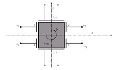
Figure 3.1: $\hat{x}-\hat{y}$ electrodes configuration around each TM.

If we assume the simple configuration in figure 3.1 with equal capacitors ($C_{i}=C,\,\forall i$) and to apply voltages $\pm V_{x,1}$ to the electrodes on the right and $\pm V_{x,2}$ to the left, provided we null the charge $Q_{\text{TM}}$ in advance, we get from (3.15):

$$\left(\sum_{j}C_{j}\right)V_{\text{TM}}=C\sum_{i}V_{i}=0\,,$$ (3.30)

hence the change in $V_{\text{TM}}$ caused by actuation voltages is $0$. Notice both the electrodes configuration, left and right, exert a pulling force on the TM by virtue of electrostatic induction creating odd-signed charges on the surface facing the electrodes; moreover, if we’d take $V_{x,1}=V_{x,2}$ no motion would be induced on the TM, but as soon as they are different, the TM moves along $\hat{x}$ and the capacitance varies increasing on the “winning” side and decreasing on the other by the same amount according to (3.17).

Therefore from (3.14), assuming $V_{x,2}>V_{x,1}$:

$$F_{x}=\left|\frac{\partial C}{\partial x}\right|\left(V_{x,1}^{2}-V_{x,2}^{2}\right)\,,$$ (3.31)

on the other hand, we can assume the usual spring-like coupling to model the stiffness as:

$$\omega_{\text{p,act},x}^{2}=-\frac{1}{m}\frac{\partial F}{\partial x}=\frac{1}{2}\sum_{j}\frac{\partial^{2}C_{j}}{\partial x^{2}}\left(V_{j}-V_{\text{TM}}\right)^{2}\,,$$ (3.32)

and under the same assumptions as before:

$$\omega_{\text{p,act},x}^{2}=\frac{1}{m}\left|\frac{\partial^{2}C}{\partial x^{2}}\right|\left(V_{x,1}^{2}+V_{x,2}^{2}\right)\,,$$ (3.33)

because the second derivative of the capacitance has the same sign for both sides, no matter the dominance of $V_{x,1}$ or $V_{x,2}$. The last equation defines a family of circles with radius of constant stiffness $\sqrt{\left|\omega_{\text{p,act},x}^{2}\right|}$ in the $V_{x,i}$ space (see picture 3.2) and if we’d take e.g. $V_{x,1}=V_{\text{max}}$ and $V_{x,2}=0$, we’d get from (3.31) and (3.33):

$$F_{x,\text{max}} =\left|\frac{\partial C}{\partial x}\right|V_{\text{max}}^{2}\,,$$ (3.34)

$$\omega_{\text{p,act},x}^{2} =\frac{1}{m}\left|\frac{\partial^{2}C}{\partial x^{2}}\right|V_{\text{max}}^{2}\,,$$ (3.35)

hence

$$\omega_{\text{p,act},x}^{2}=\frac{F_{x,\text{max}}}{m}\frac{\left|\frac{\partial^{2}C}{\partial x^{2}}\right|}{\left|\frac{\partial C}{\partial x}\right|}\,.$$ (3.36)

By placing the expressions (3.17) and (3.18) for the first and second derivatives of $C$ into the latter, we’d get:

$$\omega_{\text{p,act},x}^{2}=a_{x,\text{max}}\frac{2}{d_{x}}\,.$$ (3.37)

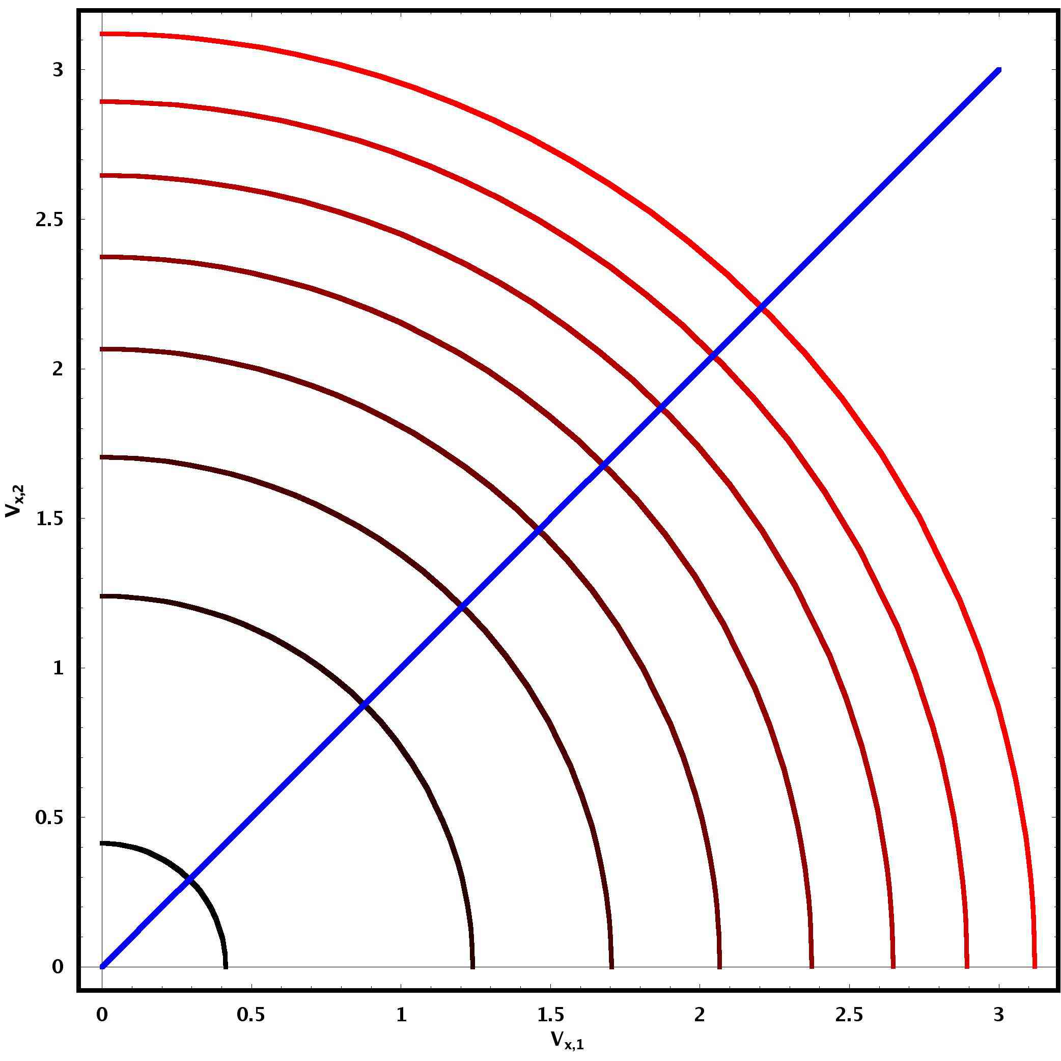
Figure 3.2: Graph of equi-stiffness curves in the electrode potentials $V_{x,i}$. The larger the stiffness, the more red-tinged the curves. The blue line represents equal voltages - therefore no forces - applied. Employed value of capacitance is the sensor’s.

The former construction can be extended to the other orthogonal electrodes configurations around each TM and allows for multiple choice of AC potentials induced on the electrodes, providing the sum of voltages amounts to $0$. Therefore any solution in $V_{j},\,\forall j$ of (3.30) with the constraint (3.32) is valid.

We can point out a number of remarks.

1. Expression (3.37) clearly shows that balance shall be made between effectiveness of the actuation and induced stiffness - independently on the DC force value - both inversely proportional to the capacitance gaps.

2. In general the TMs will carry charge $Q_{\text{TM}}\neq 0$, and in turn will have reference potential $V_{\text{TM}}\neq 0$. This facts contributes to the whole with a constant DC term in the expressions, but such an effect is not as troublesome as it might seem.

3. A tempting solution to (3.30) and (3.32) would be the AC voltage one:

   $$V_{x,1}=V_{\text{max}}\sin\omega t\,,\qquad V_{x,2}=V_{\text{max}}\cos\omega t\,,$$ (3.38)

   given a pulsation $\omega$. Notice in presence of non-zero charge of the TM the quadratic dependence of force and stiffness on the voltage foresees the creating of the mentioned DC term, plus an extra AC term at frequency $2\omega$. At high frequency neither of them is capable of inducing rotation or spurious dynamical effects on the TM due to TM inertia. Care must be taken then to bias the TM with a voltage whose frequency be outside the MBW. For LISA and LTP the MBW ranges roughly between $1\,\mathrm{mHz}$ and $1\,\mathrm{Hz}$, biasing with $\omega>100\,\mathrm{Hz}$ ensures respecting the constraints.

4. A very important feature of the strategy, which is also transparent from formulae, is that when $V_{x,1}=V_{x,2}$ no force will be present, but positive stiffness spring will be there anyway. Such a noteworthy property is extremely useful in compensating negative stiffness. Moreover, the parasitic stiffness of both TMs-ISs can be matched ($\omega_{\text{p},1}^{2}=\omega_{\text{p},2}^{2}$) by means of voltage application: if one TM will be servo-ed ($F=0$) and the other suspended ($F\neq 0$) respecting (3.31) and (3.33) they will be subject to non-zero stiffness springs and tuning of $\omega^{2}_{\text{p},i}$ can be performed. As a direct result, in science mode the ${\Delta}\omega_{\text{p}}^{2}$-modulated term in (1.101) can be annihilated as (1.102) shows and the residual acceleration ${\Delta}g_{x}$ measurement directly performed on $\text{IFO}({\Delta}x)$.

The procedure we described, to order one in stray voltages and upon completion with a careful rotational DOF treatment (see [46]), is named after “actuation at constant stiffness strategy” and it is highly relevant for both missions. In fact the GRS must bias the TMs to sense their position or measure their charge and actuate them to move on non-interferometer sensing, but this needs to be done at constant electrostatic stiffness (and minimal). By describing the stiffness manifold as a quadratic function of the potentials allows for finding time arrays of solutions, assuming to “fire” the capacitors with AC voltages on orthogonal directions periodically over an actuation period, a fundamental feature to reduce cross-talk holding control of the TMs. Obviously the simple $\omega_{\text{p,act},x}^{2}$ constant becomes a full stiffness matrix and a thorough optimisation of the solution is needed to ensure near-to-null convolution of the actuation signals over an actuation period. Figure 3.3 illustrates the carriers shape embedding sine and cosines voltage pulses for a designed control strategy for LTP [46].

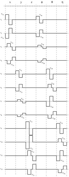
Figure 3.3: Full GRS baseline actuation sequence around slave TM.

3.3.3 Magnetics and stiffness

1. Finally, magnetic stiffness [47, 48] can be derived by means of the usual Hooke-like arguments:

   $$\omega^{2}_{\text{p,mag}}=\frac{1}{m}\left(\sqrt{6}\frac{\partial B_{x}}{\partial x}\left(\mu_{x}+\frac{\chi B_{x}L^{3}}{\mu_{0}}\right)+\sqrt{3}\frac{\partial^{2}B_{x}}{\partial x^{2}}\frac{\chi L^{3}}{\mu_{0}}\right)\,,$$ (3.39)

   where $B_{x}$ is the $\hat{x}$ component of the ${\boldsymbol{B}}$ field and the spare constants are understood. The expression can be derived from the expression of the magnetic energy density:

   $$W={\boldsymbol{\mu}}\cdot{\boldsymbol{B}}+\frac{\chi}{2\mu_{0}}{\boldsymbol{B}}\cdot{\boldsymbol{B}}\,,$$ (3.40)

   by differentiating it with respect to $x$ we derive the spring constant from the definition:

   $$\omega^{2}_{\text{p,mag}}=\frac{1}{m}\frac{\partial^{2}W}{\partial x^{2}}\,.$$ (3.41)

   Expression (3.39) is thus retrieved assuming isotropy of the permanent magnetic dipole components, so that:

   $${\boldsymbol{\mu}}^{2}=\sum_{i=1}^{3}\mu_{i}^{2}\simeq 3\mu_{x}^{2}\,,$$ (3.42)

   hence $\mu_{i}\simeq\sqrt{3}\mu_{x}$. After differentiation we integrate over the TM volume and we assume we can measure the macroscopic magnetic field and its first and second derivative. to define volume averages:

   $$\begin{split}\left\langle B_{x}\right\rangle L^{3}\simeq&\int_{V_{\text{TM}}}B_{x}(x)\operatorname{d}^{3}x\,,\\ \left\langle B_{x,x}\right\rangle L^{3}\simeq&\int_{V_{\text{TM}}}\frac{\partial}{\partial x}B_{x}(x)\operatorname{d}^{3}x\,,\\ \left\langle B_{x,xx}\right\rangle L^{3}\simeq&\int_{V_{\text{TM}}}\frac{\partial^{2}}{\partial x^{2}}B_{x}(x)\operatorname{d}^{3}x\,,\end{split}$$ (3.43)

   besides, we assume to measure $\mu_{x}$ over the whole TM volume, its dimensionality therefore being already multiplied by a factor $\mathrm{m}^{3}$. Putting all together (3.39) can be easily found.

3.3.4 Summary on stiffness

$\hat{i}$	$c(\hat{i})$	$\pi(\hat{i})$	$s(\hat{i})$	$\omega_{\text{p,sens},\hat{i}}^{2}$	$\omega_{\text{p,act},\hat{i}}^{2}$	$\omega_{\text{p,DC},\hat{i}}^{2}$
$\hat{x}_{1}$	$\hat{\phi}_{1}$	$\hat{\theta}_{1}$	$\hat{y}_{1}$, $\hat{z}_{1}$	$\omega_{\text{p,sens},x}^{2}$	$\omega_{\text{p,act},\phi_{1}}^{2}$	$\omega_{\text{p,DC},x}^{2}$
$\hat{y}_{1}$	$\hat{\theta}_{1}$	$\hat{\eta}_{1}$	$\hat{z}_{1}$, $\hat{x}_{1}$	$\omega_{\text{p,sens},y}^{2}$	$\omega_{\text{p,act},\theta_{1}}^{2}$	$\omega_{\text{p,DC},y}^{2}$
$\hat{z}_{1}$	$\hat{\eta}_{1}$	$\hat{\phi}_{1}$	$\hat{x}_{1}$, $\hat{y}_{1}$	$\omega_{\text{p,sens},z}^{2}$	$\omega_{\text{p,act},\eta_{1}}^{2}$	$\omega_{\text{p,DC},z}^{2}$
$\hat{\theta}_{1}$	$\hat{y}_{1}$	$\hat{x}_{1}$	$\hat{z}_{1}$, $\hat{x}_{1}$	$\nicefrac{{3}}{{2}}\sum_{s(\hat{i})}\omega_{\text{p,sens},s(\hat{i})}^{2}$	$\omega_{\text{p,act},\theta_{1}}^{2}$	$\nicefrac{{3}}{{2}}\sum_{s(\hat{i})}\omega_{\text{p,DC},s(\hat{i})}^{2}$
$\hat{\eta}_{1}$	$\hat{z}_{1}$	$\hat{y}_{1}$	$\hat{x}_{1}$, $\hat{y}_{1}$	$\nicefrac{{3}}{{2}}\sum_{s(\hat{i})}\omega_{\text{p,sens},s(\hat{i})}^{2}$	$\omega_{\text{p,act},\eta_{1}}^{2}$	$\nicefrac{{3}}{{2}}\sum_{s(\hat{i})}\omega_{\text{p,DC},s(\hat{i})}^{2}$
$\hat{\phi}_{1}$	$\hat{x}_{1}$	$\hat{z}_{1}$	$\hat{y}_{1}$, $\hat{z}_{1}$	$\nicefrac{{3}}{{2}}\sum_{s(\hat{i})}\omega_{\text{p,sens},s(\hat{i})}^{2}$	$\omega_{\text{p,act},\phi_{1}}^{2}$	$\nicefrac{{3}}{{2}}\sum_{s(\hat{i})}\omega_{\text{p,DC},s(\hat{i})}^{2}$
$\hat{x}_{2}$	$\hat{\phi}_{2}$	$\hat{\theta}_{2}$	$\hat{y}_{2}$, $\hat{z}_{2}$	$\omega_{\text{p,sens},x}^{2}$	$\omega_{\text{p,act},\phi_{2}}^{2}+\omega_{\text{p,act},x_{2}}^{2}$	$\omega_{\text{p,DC},x}^{2}$
$\hat{y}_{2}$	$\hat{\theta}_{2}$	$\hat{\eta}_{2}$	$\hat{z}_{2}$, $\hat{x}_{2}$	$\omega_{\text{p,sens},y}^{2}$	$\omega_{\text{p,act},\theta_{2}}^{2}+\omega_{\text{p,act},y_{2}}^{2}$	$\omega_{\text{p,DC},y}^{2}$
$\hat{z}_{2}$	$\hat{\eta}_{2}$	$\hat{\phi}_{2}$	$\hat{x}_{2}$, $\hat{y}_{2}$	$\omega_{\text{p,sens},z}^{2}$	$\omega_{\text{p,act},\eta_{2}}^{2}+\omega_{\text{p,act},z_{2}}^{2}$	$\omega_{\text{p,DC},z}^{2}$
$\hat{\theta}_{2}$	$\hat{y}_{2}$	$\hat{x}_{2}$	$\hat{z}_{2}$, $\hat{x}_{2}$	$\nicefrac{{3}}{{2}}\sum_{s(\hat{i})}\omega_{\text{p,sens},s(\hat{i})}^{2}$	$\omega_{\text{p,act},\theta_{2}}^{2}+\nicefrac{{3}}{{2}}\sum_{s(\hat{i})}\omega_{\text{p,act},s(\hat{i})}^{2}$	$\nicefrac{{3}}{{2}}\sum_{s(\hat{i})}\omega_{\text{p,DC},s(\hat{i})}^{2}$
$\hat{\eta}_{2}$	$\hat{z}_{2}$	$\hat{y}_{2}$	$\hat{x}_{2}$, $\hat{y}_{2}$	$\nicefrac{{3}}{{2}}\sum_{s(\hat{i})}\omega_{\text{p,sens},s(\hat{i})}^{2}$	$\omega_{\text{p,act},\eta_{2}}^{2}+\nicefrac{{3}}{{2}}\sum_{s(\hat{i})}\omega_{\text{p,act},s(\hat{i})}^{2}$	$\nicefrac{{3}}{{2}}\sum_{s(\hat{i})}\omega_{\text{p,DC},s(\hat{i})}^{2}$
$\hat{\phi}_{2}$	$\hat{x}_{2}$	$\hat{z}_{2}$	$\hat{y}_{2}$, $\hat{z}_{2}$	$\nicefrac{{3}}{{2}}\sum_{s(\hat{i})}\omega_{\text{p,sens},s(\hat{i})}^{2}$	$\omega_{\text{p,act},\phi_{2}}^{2}+\nicefrac{{3}}{{2}}\sum_{s(\hat{i})}\omega_{\text{p,act},s(\hat{i})}^{2}$	$\nicefrac{{3}}{{2}}\sum_{s(\hat{i})}\omega_{\text{p,DC},s(\hat{i})}^{2}$

Table 3.2: Conjugated and co-sensed DOF versus stiffness. From left to right: the $\hat{i}$ column represents the variable, $c(\hat{i})$ the one which is sensed by the same GRS electrode surface $s(\hat{i})$, $\pi(\hat{i})$ is the dynamically conjugated DOF. Sensing, actuation and DC-force stiffness depends on the choice of electrodes and the conjugation.

We can write, for every DOF, the following general formula with reference to table 3.2:

$$\omega_{\text{p},\hat{i},\hat{i}}^{2}\doteq\omega_{\text{p,mag}}^{2}+\omega^{2}_{\text{p,grav},\hat{i},\hat{i}}+\omega_{\text{p,act},\hat{i}}^{2}+\omega_{\text{p,DC},\hat{i}}^{2}+\omega_{\text{p,sens},\hat{i}}^{2}\,,$$ (3.44)

so that, e.g. for the $\hat{x}_{1}$ full stiffness we’d get:

$$\omega_{\text{p},x_{1},x_{1}}^{2}=\omega_{\text{p,mag}}^{2}+\omega^{2}_{\text{p,grav},xx}+\omega_{\text{p,act},\theta_{1}}^{2}+\omega_{\text{p,DC},x_{1}}^{2}+\omega_{\text{p,sens},x_{1}}^{2}\,,$$ (3.45)

or, for $\hat{\eta}_{2}$:

$$\begin{split}\omega_{\text{p},\eta_{2},\eta_{2}}^{2}=&\omega_{\text{p,mag}}^{2}+\omega^{2}_{\text{p,grav},\eta_{2}\eta_{2}}+\omega_{\text{p,act},\eta_{2}}^{2}+\frac{3}{2}\left(\omega_{\text{p,act},x_{2}}^{2}+\omega_{\text{p,act},y_{2}}^{2}\right)+\\ &+\frac{3}{2}\left(\omega_{\text{p,DC},x_{2}}^{2}+\omega_{\text{p,DC},y_{2}}^{2}\right)+\frac{3}{2}\left(\omega_{\text{p,sens},x_{2}}^{2}+\omega_{\text{p,sens},y_{2}}^{2}\right)\,.\end{split}$$ (3.46)

To evaluate the difference in stiffness we cannot assume it to be due to actuation only. In this exposition we are interested to show this difference only for linear DOF, and we can write in general:

$${\Delta}\omega_{\text{p},\hat{i}}^{2}\doteq\lambda_{\hat{i}}\left(\frac{\omega^{2}_{\text{p,grav},\hat{i},\hat{i}}}{5}+\sqrt{2}\left(\omega_{\text{p,act},c(\hat{i})}^{2}+\omega_{\text{p,mag}}^{2}+\omega_{\text{p,DC},\hat{i}}^{2}\right)+\frac{\omega_{\text{p,sens},\hat{i}}^{2}}{10}+\omega_{\text{p,act},\hat{i}}^{2}\right)\,,$$ (3.47)

where $\lambda_{\hat{i}}$ is a weight which is $\nicefrac{{1}}{{2}}$ along $\hat{y}$ and $\hat{z}$ but $1$ for $\hat{x}$ where we demand a stricter performance. As seen we assume to compensate gravity gradients up to $20\%$, sensing stiffness to $10\%$ but we have to retain DC, magnetics and angular-actuation stiffness effects, though correlated. Actuation stiffness is taken as it is. For the $\hat{x}$ direction we can apply the former and write:

$${\Delta}\omega_{\text{p},x}^{2}=\frac{\omega^{2}_{\text{p,grav},xx}}{5}+\sqrt{2}\left(\omega_{\text{p,act},\phi}^{2}+\omega_{\text{p,mag}}^{2}+\omega_{\text{p,DC},x}^{2}\right)+\frac{\omega_{\text{p,sens},x}^{2}}{10}+\omega_{\text{p,act},x}^{2}\,,$$ (3.48)

With reference to the main signal equation (3.2) we can see that the rôle of difference of stiffness cannot be neglected or thought as being $0$, due to the term in $\nicefrac{{g_{\text{SC,x}}}}{{{\omega_{\text{df},x}^{2}}}}$ and noise in readout.

Description	Name	Value	Dimensions
Sensing stiffness	$\omega^{2}_{\text{p,sens}}$	$0.442\times 10^{-7}$	$\nicefrac{\mathrm{1}}{\mathrm{s^{2}}}$
Actuation stiffness	$\omega^{2}_{\text{p,act}}$	$0.501\times 10^{-6}$	$\nicefrac{\mathrm{1}}{\mathrm{s^{2}}}$
Rotation actuation stiffness	$\omega^{2}_{\text{p,rot}}$	$0.767\times 10^{-8}$	$\nicefrac{\mathrm{1}}{\mathrm{s^{2}}}$
Magnetic stiffness	$\omega^{2}_{\text{p,mag}}$	$0.578\times 10^{-8}$	$\nicefrac{\mathrm{1}}{\mathrm{s^{2}}}$
DC voltage stiffness	$\omega^{2}_{\text{p,DC}}$	$0.726\times 10^{-8}$	$\nicefrac{\mathrm{1}}{\mathrm{s^{2}}}$
Total stiffness, TM1, nominal	$\omega^{2}_{\text{p,1}}$	$0.565\times 10^{-6}$	$\nicefrac{\mathrm{1}}{\mathrm{s^{2}}}$
Total stiffness, TM2, nominal	$\omega^{2}_{\text{p,2}}$	$0.107\times 10^{-5}$	$\nicefrac{\mathrm{1}}{\mathrm{s^{2}}}$
Difference of stiffness	${\Delta}\omega^{2}_{\text{p,tot}}$	$0.574\times 10^{-6}$	$\nicefrac{\mathrm{1}}{\mathrm{s^{2}}}$

Table 3.3: Stiffness, summary

3.4 Inertial sensor displacement noise

Description	Name	Value	Dimensions
DC differential acceleration $\hat{x}$	$g_{\text{DC},x}$	$1.\times 10^{-9}$	$\nicefrac{\mathrm{m}}{\mathrm{s^{2}}}$
DC differential acceleration $\hat{y}$	$g_{\text{DC},y}$	$5.\times 10^{-10}$	$\nicefrac{\mathrm{m}}{\mathrm{s^{2}}}$
DC differential acceleration $\hat{z}$	$g_{\text{DC},z}$	$5.\times 10^{-10}$	$\nicefrac{\mathrm{m}}{\mathrm{s^{2}}}$
DC torque/moment of inertia $\hat{\theta}$	$g_{\text{DC},\theta}$	$1.\times 10^{-9}$	$\nicefrac{\mathrm{1}}{\mathrm{s^{2}}}$
DC torque/moment of inertia $\hat{\eta}$	$g_{\text{DC},\eta}$	$2.\times 10^{-9}$	$\nicefrac{\mathrm{1}}{\mathrm{s^{2}}}$
DC torque/moment of inertia $\hat{\phi}$	$g_{\text{DC},\phi}$	$1.\times 10^{-9}$	$\nicefrac{\mathrm{1}}{\mathrm{s^{2}}}$

Table 3.4: Tolerable maximal differential DC accelerations for linear DOF and maximal DC torques per unit moment of inertia.

Description	Name	Value	Dimensions
Gravity gradient $\hat{x}$	$\omega^{2}_{\text{p,grav},\text{xx}}$	$5.\times 10^{-7}$	$\nicefrac{\mathrm{1}}{\mathrm{s^{2}}}$
Gravity gradient $\hat{y}$	$\omega^{2}_{\text{p,grav},\text{yy}}$	$5.\times 10^{-8}$	$\nicefrac{\mathrm{1}}{\mathrm{s^{2}}}$
Gravity gradient $\hat{z}$	$\omega^{2}_{\text{p,grav},\text{zz}}$	$-5.5\times 10^{-7}$	$\nicefrac{\mathrm{1}}{\mathrm{s^{2}}}$
Gravity gradient $\hat{\theta}$	$\omega^{2}_{\text{p,grav},\theta\theta}$	$1.\times 10^{-8}$	$\nicefrac{\mathrm{1}}{\mathrm{s^{2}}}$
Gravity gradient $\hat{\eta}$	$\omega^{2}_{\text{p,grav},\eta\eta}$	$1.\times 10^{-8}$	$\nicefrac{\mathrm{1}}{\mathrm{s^{2}}}$
Gravity gradient $\hat{\phi}$	$\omega^{2}_{\text{p,grav},\phi\phi}$	$1.\times 10^{-8}$	$\nicefrac{\mathrm{1}}{\mathrm{s^{2}}}$

Table 3.5: Gravity gradients

The uncertainty coming from the position detectors induces a displacement noise. Due to the existence of the drag-free control loop, this can be converted into a force noise via proper transfer functions. In this scenario it is of capital importance to gain knowledge about the parasitic stiffness that couples both the TMs to the SC. Moreover, the control strategy is important to understand the origin of the noise: in science mode, since only one TM is actuated and served by the SC, only the noise coming from the sensing TM matters.

Dealing with an electrostatic detector, we’d like to point out two reading rules for the following formulae:

1. In general, our electrostatic detector/actuator is nothing but a differential inductive bridge. A capacitive imbalance caused by a TM displacement creates a differential transformer current according to eq. (3.16), with the secondary current amplified and read out with lock-in detection. We choose the bridge injection capacitor $C_{\text{inj}}$ value so to bring the bridge to resonance at $100\,\mathrm{kHz}$ excitation frequency, with the main purpose of minimising the amplifier noise. If the model is simplified to a series RLC circuit, then the complex impedance of the full circuit is

   $$Z=R+\frac{1}{\imath\omega C_{\text{inj}}}+\imath\omega 2L_{i}\,,$$ (3.49)

   where the factor $2$ comes from the presence of 2 inductors in the bridge and $L_{i}$ is the primary inductance of the single inductor. Resonance condition is achieved when $\operatorname{Im}Z=0$, thus:

   $$\omega_{\text{inj,res}}^{2}=\frac{1}{2C_{\text{inj}}L_{i}}\,,$$ (3.50)

   from which:

   $$C_{\text{inj}}=\frac{1}{2\omega_{\text{inj}}^{2}L_{i}}\,.$$ (3.51)

   We named $\omega_{\text{inj}}=2\pi f_{\text{inj}}$ as the readout bias frequency, such that $f_{\text{inj}}=100\,\mathrm{kHz}$. Parameters can be checked in table 3.8, a value of $C_{\text{inj}}$ can be checked in table 3.6. In the real circuit (see figure 3.4) more capacitance’s are called in place, their effect being to shift the resonance. We assume nevertheless this correction to be small and summarise it in the $Q$-factor in the following (see expression (3.57)).

2. Concerning thermal noise, dielectric or inductive losses can be caused by many different phenomena: our general approach will be to discuss them in a sort of intuitive manner rather then tediously deduce each formula. An example on capacitance may mark the way: according to Nyquist theory, the thermal power spectrum of a dissipative dynamical system J is a function of absolute temperature and impedance $Z_{j}$ as follows:

   $$S^{\nicefrac{{1}}{{2}}}_{\text{J}}=\sqrt{4k_{\text{B}}T\operatorname{Re}Z_{\text{J}}}\,,$$ (3.52)

   where $k_{\text{B}}$ is Boltzmann’s constant. In the case of dielectric loss caused by electrode surface contamination we can model the presence of impurities and spots by a macroscopic dimensionless “loss angle” $\delta$, such that $C\to C(1+\imath\delta_{C})$, hence, since a capacitor impedance is

   $$Z=\frac{1}{\imath\omega C(1+\imath\delta_{C})}\,,$$ (3.53)

   we get

   $$S^{\nicefrac{{1}}{{2}}}_{\text{diel}}=\sqrt{4k_{\text{B}}T\frac{\delta_{C}}{\omega C}}\,.$$ (3.54)

   Similar deductions apply for lossy inductance’s $L\to L(1+\imath\delta_{L})$. Effects like this perturb the readout directly affecting position reading (this is the case of patches over the capacitors plates, e.g.).

Readout noise is made of two different kinds of contribution: correlated and uncorrelated. Distinction is made on the basis of the source of the phenomena and these latter may or may not share correlations to the same source. Moreover, a distinction will be made on the phase shift the current will pick up at $V_{\text{out}}$ with respect to the original phase at $V_{\text{inj}}$ as a result of the capacitance or inductive electronics it will pass through in the circuitry. Notice at this level that magnetic flux conservation and the fact that primary and secondary inductors are equal in the employed transformer doesn’t create any phase delay due to induction.

Description	Name	Value	Dimensions
Parallel capacitance to ground	$C_{\text{inj}}$	$0.486\times 10^{-9}$	$\mathrm{F}$
Readout Q factor	$Q$	$0.985\times 10^{2}$	$1$

Table 3.6: Summary of derived quantities

3.4.1 Electric correlated

Due to the specific form of the electrostatic readout devices three main sources can be spelled in this section. The readout bridge can be split into three subsystems: the capacitors with the transformer, the amplifier and the actuation circuitry. Hence there’s noise - in phase - produced in the transformer, deeply caused by thermal excitation of matter states, voltage noise in the amplifier, and actuation noise.

Transformer thermal noise, in phase.

In spite of its small contribution the thermal noise induced by the transformer has a PSD expression which is worth discussing because of the functional form. Let’s write it down:

$$S^{\nicefrac{{1}}{{2}}}_{x,\text{trip}}=\frac{d_{x}}{\sqrt{2}}\frac{1}{V_{\text{inj}}Q}\sqrt{\frac{4k_{B}T}{\omega_{\text{inj}}C_{\text{sens}}}\left(\frac{1}{2\omega_{\text{inj}}^{2}L_{i}C_{\text{sens}}Q}\right)}\,,$$ (3.55)

where

$d_{x}$

is the sensing gap along the $\hat{x}$ direction,

$C_{\text{sens}}$

is the single electrode sensing capacity,

$V_{\text{inj}}$

is the TM sensing bias voltage amplitude (at $100\,\mathrm{kHz}$),

$L_{i}$

is the single inductor primary inductance,

$T$

is the absolute temperature,

$k_{B}$

is Boltzmann constant,

$C_{\text{inj}}$

parallel capacitance to ground, expressed at resonance by formula (3.51).

Nominal values of the former constants can be found in tables 3.7 and 3.8. The value of $S^{\nicefrac{{1}}{{2}}}_{x,\text{trip}}$ is shown in table 3.12.

We already discussed the relation between voltage PSD and displacement PSD in (3.12). The reason of the $d_{x}$ pre-factor lies there. We then recognise the dependence on $\sqrt{4k_{\text{B}}T}$ and the square root of the real part of the impedance: intuitively we expect an inverse dependence on $V_{\text{inj}}$, something we’ll retrieve in all thermal voltage noise formulae in the following; the ratio $\nicefrac{{C_{\text{sens}}}}{{C_{\text{inj}}}}$ is another common feature, a pure number hinting to how strong is the capacitance ratio between ground and the bridge.

$Q$ is the readout $Q$-factor, expressed by:

$$Q=2\omega_{\text{inj}}^{2}L_{i}\left(C_{\text{cable}}\delta_{\text{cable}}+C_{\text{par}}\delta_{\text{par}}\right)+\delta_{L_{i}}\,,$$ (3.56)

by employing expression (3.51) for $C_{\text{inj}}$, we find the algebraic inverse of $Q$ gets an interesting functional form:

$$\frac{1}{Q}=\frac{C_{\text{cable}}\delta_{\text{cable}}}{C_{\text{inj}}}+\delta_{L_{i}}+\frac{C_{\text{par}}\delta_{\text{par}}}{C_{\text{inj}}}\,.$$ (3.57)

We’d like to spend a couple more words on this expression. It’s a combination of the following variables:

$\delta_{\text{par}}$

parasitic capacitance loss angle,

$C_{\text{par}}$

electrode parasitic capacitance to ground.

It is clear then that the $Q$-factor expresses an average loss factor, such as $C_{\text{inj}}Q^{-1}=\sum_{j}C_{j}\delta_{j}$, where $j$ ranges over all the conductors at play. The name “quality factor” comes on the line of the introductory discussion we went through at the beginning of the chapter. Notice the PSD is continuous in $Q$, there would be no noise if there wouldn’t be any dissipation.

Description	Name	Value	Dimensions
Single electrode sensing capacity	$C_{\text{sens}}$	$1.15\times 10^{-12}$	$\mathrm{F}$
Sensing capacity loss angle	$\delta_{\text{sens}}$	$1.\times 10^{-5}$	$1$
Electrode parasitic capacitance to ground	$C_{\text{par}}$	$2.\times 10^{-11}$	$\mathrm{F}$
Parasitic capacitance loss angle	$\delta_{\text{par}}$	$2.\times 10^{-2}$	$1$
Sensing gap x	$d_{x}$	$4.\times 10^{-3}$	$\mathrm{m}$
Sensing gap y	$d_{y}$	$2.9\times 10^{-3}$	$\mathrm{m}$
Sensing gap z	$d_{z}$	$3.5\times 10^{-3}$	$\mathrm{m}$

Table 3.7: Electrode characteristics

Description	Name	Value	Dimensions
TM sensing bias voltage amplitude ($100\,\mathrm{kHz}$)	$V_{\text{inj}}$	$0.6$	$\mathrm{V}$
Readout bias frequency	$f_{\text{inj}}=\nicefrac{{\omega_{\text{inj}}}}{{2\pi}}$	$1.\times 10^{5}$	$\mathrm{Hz}$
AC-bias relative amplitude fluctuation (@$\omega$)	$S_{\nicefrac{{{\Delta}V_{\text{AC}}}}{{V_{\text{AC}}}}}$	$\left(1.\times 10^{-4}\right)^{2}\left(\frac{2\pi\times 10^{-3}\,\mathrm{Hz}}{\omega}\right)^{2}$	$\nicefrac{\mathrm{1}}{\mathrm{Hz}}$
Single inductor primary inductance	$L_{i}$	$2.61\times 10^{-3}$	$\mathrm{Henry}$
Transformer turn ratio	$n_{o}$	$1$	$1$
Transformer core loss angle	$\delta_{L_{i}}$	$\nicefrac{{1}}{{110}}$	$1$
Transformer imbalance fluctuations	$S_{\nicefrac{{{\Delta}L_{i}}}{{L_{i}}}}$	$\left(1.\times 10^{-7}\right)^{2}\left(\frac{2\pi\times 10^{-3}\,\mathrm{Hz}}{\omega}\right)^{2}$	$\nicefrac{\mathrm{1}}{\mathrm{Hz}}$
Cable parasitic capacitance	$C_{\text{cable}}$	$3.\times 10^{-12}$	$\mathrm{F}$
Cable loss angle	$\delta_{\text{cable}}$	$4.\times 10^{-2}$	$1$
Amplifier voltage noise	$S_{V_{\text{amp}}}$	$\left(2.\times 10^{-9}\right)^{2}\left(\frac{2\pi\times 10^{-3}\,\mathrm{Hz}}{\omega}\right)^{2}$	$\nicefrac{\mathrm{V^{2}}}{\mathrm{Hz}}$
Amplifier current noise	$S_{I_{\text{amp}}}$	$\left(1.\times 10^{-14}\right)^{2}\left(\frac{2\pi\times 10^{-3}\,\mathrm{Hz}}{\omega}\right)^{2}$	$\nicefrac{\mathrm{A^{2}}}{\mathrm{Hz}}$
Feedback capacitor	$C_{\text{fb}}$	$1.\times 10^{-11}$	$\mathrm{F}$
Feedback capacitor loss	$\delta_{C_{\text{fb}}}$	$1.\times 10^{-2}$	$1$
Feedback capacitance relative fluctuation	$S_{\nicefrac{{{\Delta}C_{\text{fb}}}}{{C_{\text{fb}}}}}$	$\left(1.\times 10^{-5}\right)^{2}$	$\nicefrac{\mathrm{1}}{\mathrm{Hz}}$
Effective bridge output offset	${\Delta}x_{\text{bo}}$	$2.\times 10^{-6}$	$\mathrm{m}$

Table 3.8: Readout characteristics

Amplifier voltage noise, in phase.

The same arguments applied before to build the transformer thermal noise apply here as well: hence the turn ratio factor will appear and the noise PSD will be linearly dependent upon it, i.e. if the voltage get amplified, any noise voltage will be as well by means of the same physics. The distance/capacitance pre-factor is unmodified but - as can be seen in the circuit scheme 3.4 - a feedback capacitor is inserted and its capacitance modulates the noise linearly. In formula:

$$S^{\nicefrac{{1}}{{2}}}_{x,\text{ampip}}=\frac{d_{x}}{\sqrt{2}}\frac{1}{V_{\text{inj}}}\frac{C_{\text{fb}}}{\sqrt{2}C_{\text{sens}}}n_{o}\sqrt{S_{V_{\text{amp}}}}\,,$$ (3.58)

where - apart from already mentioned variables - we can distinguish between:

$n_{0}$

representing the transformer turn ratio,

$C_{\text{fb}}$

being the feedback capacitance,

$S_{V_{\text{amp}}}$

the amplifier voltage noise.

Again, values can be retrieved from tables 3.7 and 3.8. The value of $S^{\nicefrac{{1}}{{2}}}_{x,\text{ampip}}$ is shown in table 3.12.

Actuation noise at $100\,\mathrm{kHz}$.

Actuation noise at $100\,\mathrm{kHz}$ is a contribution one order of magnitude larger than the former two mentioned in this section. No wonder in deducing the formula, which we state as:

$$S^{\nicefrac{{1}}{{2}}}_{x,\text{act100}}=\frac{d_{x}}{\sqrt{2}}\frac{1}{V_{\text{inj}}}\frac{C_{\text{inj}}}{C_{\text{sens}}}\gamma_{o,100\mathrm{kHz}}\sqrt{S_{V_{\text{act}}}}\,,$$ (3.59)

where

$S_{V_{\text{act}}}$

is the actuation voltage noise at output ($100\,\mathrm{kHz}$ and MBW);

$\gamma_{o,100\mathrm{kHz}}$

is the actuation filter open loop transfer. Transfer functions always appear unabridged homogeneously multiplying PSDs, dimensionless ones.

Values can be retrieved from tables 3.7 and 3.8 together with 3.9. The value of $S^{\nicefrac{{1}}{{2}}}_{x,\text{act100}}$ is to be found in table 3.12.

Description	Name	Value	Dimensions
Actuation amplitude relative fluctuation	$S_{\nicefrac{{{\Delta}V_{\text{act}}}}{{V_{\text{act}}}}}$	$\left(2.\times 10^{-6}\right)^{2}\left(\frac{2\pi\times 10^{-3}\,\mathrm{Hz}}{\omega}\right)^{2}$	$\nicefrac{\mathrm{1}}{\mathrm{Hz}}$
Actuation voltage noise at output($100\,\mathrm{kHz}$ and MBW)	$S_{V_{\text{act}}}$	$\left(1.\times 10^{-6}\right)^{2}\left(\frac{2\pi\times 10^{-3}\,\mathrm{Hz}}{\omega}\right)^{2}$	$\nicefrac{\mathrm{V^{2}}}{\mathrm{Hz}}$
Actuation filter open loop transfer	$\gamma_{o,100\mathrm{kHz}}$	$1.\times 10^{-4}$	$1$
Actuation filter closed loop transfer	$\gamma_{c,100\mathrm{kHz}}$	$1.\times 10^{-4}$	$1$
Actuation filter impedance	$Z_{\text{act}}$	$10.$	$\mathrm{\Omega}$

Table 3.9: Actuation characteristics

Figure 3.4: Sensing bridge of the type LTP will be equipped with and similar to sensing devices of torsion pendulum facility at the University of Trento. The set of electrodes on the right mimics the TM, with charge $q$, the transformer in the middle with turn ratio $n_{0}$, the amplifier on the right. The actuation circuit is shown at top and bottom.

3.4.2 Electric uncorrelated

All values can be retrieved from table 3.12. Here we have:

Transformer thermal noise, out of phase.

The out of phase transformer thermal noise is a highly relevant contribution to the noise PSD, amounting to magnitude $10^{-9}$. No difference in deducing or building the formula rather than eq. (3.55), but obviously we get rid of the $\nicefrac{{1}}{{Q}}$ pre-factor since we are now looking for out-of-phase contributions:

$$S^{\nicefrac{{1}}{{2}}}_{x,\text{trop}}=\frac{d_{x}}{\sqrt{2}V_{\text{inj}}}\sqrt{\frac{4k_{B}T}{\omega_{\text{inj}}C_{\text{sens}}}\left(\frac{1}{2\omega_{\text{inj}}^{2}L_{i}C_{\text{sens}}Q}\right)}\,,$$ (3.60)

Amplifier voltage noise, out of phase

$$S^{\nicefrac{{1}}{{2}}}_{x,\text{ampop}}=\frac{d_{x}}{\sqrt{2}}\frac{1}{V_{\text{inj}}}\frac{C_{\text{fb}}}{\sqrt{2}C_{\text{sens}}}\frac{1}{\left(n_{o}\omega_{\text{inj}}^{2}L_{i}C_{\text{fb}}Q\right)}\sqrt{S_{V_{\text{amp}}}}\,,$$ (3.61)

Amplifier current noise, out of phase

$$S^{\nicefrac{{1}}{{2}}}_{x,\text{curop}}=\frac{d_{x}}{\sqrt{2}}\frac{\sqrt{S_{I_{\text{amp}}}}}{V_{\text{inj}}}\frac{n_{o}}{\sqrt{2}\omega_{\text{inj}}C_{\text{sens}}}\,,$$ (3.62)

Feedback capacitor current noise, in phase

$$S^{\nicefrac{{1}}{{2}}}_{x,\text{cufb}}=\frac{d_{x}}{\sqrt{2}}\frac{n_{o}}{V_{\text{inj}}}\sqrt{\frac{2k_{B}T\delta_{C_{\text{fb}}}}{\omega_{\text{inj}}C_{\text{fb}}}}\,,$$ (3.63)

Differential transformer imbalance, in phase

$$S^{\nicefrac{{1}}{{2}}}_{x,\text{dt}}=\frac{d_{x}}{\sqrt{2}}\frac{\sqrt{S_{\nicefrac{{{\Delta}L_{i}}}{{L_{i}}}}}}{4}\,,$$ (3.64)

Oscillator amplifier amplitude noise

$$S^{\nicefrac{{1}}{{2}}}_{x,\text{osc}}={\Delta}x_{\text{bo}}\sqrt{S_{\nicefrac{{{\Delta}V_{\text{AC}}}}{{V_{\text{AC}}}}}}\,,$$ (3.65)

Feedback capacitor instability noise

$$S^{\nicefrac{{1}}{{2}}}_{x,\text{Cfb}}=\frac{{\Delta}x_{\text{bo}}}{\sqrt{2}}\sqrt{S_{\nicefrac{{{\Delta}C_{\text{fb}}}}{{C_{\text{fb}}}}}}\,,$$ (3.66)

3.4.3 Thermal correlated distortion

The thermal displacement noise formula is easily deductible from thermal dilatation principles. Given a linear dilatation model:

$${\Delta}x\simeq\alpha L_{0}{\Delta}T\,,$$ (3.67)

where ${\Delta}x$ is the dilatation, $L_{0}$ the starting length, $\alpha$ some dilatation coefficient and ${\Delta}T$ the temperature excursion, we simply have to switch to PSD space as follows:

$$S^{\nicefrac{{1}}{{2}}}_{x,\text{th}}=\alpha_{\text{th}}\left(\frac{L}{2}\right)\sqrt{S_{{\Delta}T}}\,.$$ (3.68)

Constants and descriptions can be found in table 3.15. Notice since in this case we are dealing with a temperature difference fluctuation $S_{{\Delta}T}$, we consider a geometric factor of $\nicefrac{{1}}{{2}}$ in the baseline length. The final value of $S^{\nicefrac{{1}}{{2}}}_{x,\text{th}}$ is to be found in table 3.12.

3.4.4 Contribution from forces on the SC

Again a careful inspection of (3.2) reveals the contributions of forces coming from the SC to sensor displacement noise can be summarised in the term:

$$\left(\omega^{2}_{\text{p},2}-\omega^{2}_{\text{p},1}\right)\frac{g_{\text{SC,x}}}{\omega_{\text{df},x}^{2}}\,.$$ (3.69)

Therefore, in terms of the PSD of forces acting on the SC:

$$S^{\nicefrac{{1}}{{2}}}_{x,\text{SC}}=\frac{\left|\omega^{2}_{\text{p},2}-\omega^{2}_{\text{p},1}\right|}{\left|\omega_{\text{df},x}^{2}\right|}\frac{\sqrt{S_{\text{SC}}}}{m_{\text{SC}}}\,.$$ (3.70)

The value is reported in table 3.12, values of constants and their meaning can be found in table 3.10, the form of $\omega^{2}_{\text{df},x}$ can be retrieved from (2.145) and table 2.5.

Description	Name	Value	Dimensions
Forces on SC	$S_{\text{SC}}$	$(5.0\times 10^{-6})^{2}\left(2\pi\times\frac{10^{-3}\,\mathrm{Hz}}{\omega}\right)^{2}$	$\nicefrac{\mathrm{N^{2}}}{\mathrm{Hz}}$
SC mass	$m_{\text{SC}}$	$476.$	$\mathrm{kg}$
SC effective radius	$R_{\text{SC}}$	$1$	m

Table 3.10: SC characteristics and estimate of external forces

3.4.5 Summary of displacement noise, drag-free noise

At the end of the analysis the contributions will be summed quadratically, assuming they are basically uncorrelated or weakly correlated anyway:

$$S^{\nicefrac{{1}}{{2}}}_{x,j}S^{\nicefrac{{1}}{{2}}}_{x,k}\ll S_{x,j}+S_{x,k}\,.$$ (3.71)

It turns out, in estimating the total sensor noise, that this procedure gives the worst estimate of the effects, therefore being preferable in planning phase; moreover, due to the very local nature of the disturbances, this is also physically meaningful. We have then, for the total noise on the sensor:

$$S_{x,\text{sens}}=S_{x,\text{corr}}+S_{x,\text{uncorr}}+S_{x,\text{th}}\,,$$ (3.72)

where

$$S_{x,\text{corr}}=S_{x,\text{trip}}+S_{x,\text{ampip}}+S_{x,\text{act100}}\,,$$ (3.73)

and

$$\begin{split}S_{x,\text{uncorr}}=&S_{x,\text{trop}}+S_{x,\text{ampop}}+S_{x,\text{curop}}+\\ &+S_{x,\text{cufb}}+S_{x,\text{dt}}+S_{x,\text{osc}}+S_{x,\text{Cfb}}\,,\end{split}$$ (3.74)

while, if we take into account the forces acting on the SC, we can compute the total drag-free displacement noise:

$$S_{x,\text{tot}}=S_{x,\text{SC}}+S_{x,\text{sens}}\,.$$ (3.75)

Figures are to be retrieved from table 3.12.

This long discussion about displacement noise formerly carried on is motivated by the drag-free control loop. Acceleration noise is enlarged by displacement noise converted into acceleration via the difference of stiffness constant ${\Delta}\omega_{\text{p}}^{2}$ - see eq. (3.48) - so that the displacement spectrum gets converted into an acceleration one:

$$S^{\nicefrac{{1}}{{2}}}_{a,\text{dragfree}}=\left|{\Delta}\omega_{\text{p},x}^{2}\right|S_{x,\text{tot}}^{\nicefrac{{1}}{{2}}}\,,$$ (3.76)

whose value can be found in table 3.33.

Description	Name	Value	Dimensions
Stray DC electrode potential	$V_{\text{stray}}$	$3.\times 10^{-2}$	$\mathrm{V}$
Charge events rate	$\lambda$	$5.\times 10^{2}$	$\mathrm{Hz}$
Test-mass charge/electron charge	$q_{0}$	$1.\times 10^{7}$	$1$
Shielding factor	$\alpha_{\text{sh}}$	$1.\times 10^{-3}$	$1$
In-band voltage fluctuations	$S_{V_{\text{ib}}}$	$\left(1.\times 10^{-4}\right)^{2}\left(2\pi\times\frac{10^{-3}\,\mathrm{Hz}}{\omega}\right)^{2}$	$\nicefrac{\mathrm{V^{2}}}{\mathrm{Hz}}$
Maximum AC voltage within electrodes	$V_{\text{AC}}$	$1.$	$\mathrm{V}$
AC voltage noise	$S_{V_{\text{AC}}}$	$\left(1.\times 10^{-7}\right)^{2}\left(2\pi\times\frac{10^{-3}\,\mathrm{Hz}}{\omega}\right)^{2}$	$\nicefrac{\mathrm{V^{2}}}{\mathrm{Hz}}$

Table 3.11: Voltage and charge characteristics

Description	Name	Value $(\nicefrac{\mathrm{m}}{\mathrm{\sqrt{Hz}}})$
Transformer thermal noise. In-phase	$S^{\nicefrac{{1}}{{2}}}_{x,\text{trip}}$	$1.49\times 10^{-11}$
Amplifier voltage noise. In-phase	$S^{\nicefrac{{1}}{{2}}}_{x,\text{ampip}}$	$5.79\times 10^{-11}$
Actuation noise at 100 kHz	$S^{\nicefrac{{1}}{{2}}}_{x,\text{act100}}$	$1.99\times 10^{-10}$
Transformer thermal noise. Out-of-phase	$S^{\nicefrac{{1}}{{2}}}_{x,\text{trop}}$	$1.46\times 10^{-9}$
Amplifier voltage noise. Out-of-phase	$S^{\nicefrac{{1}}{{2}}}_{x,\text{ampop}}$	$5.72\times 10^{-11}$
Amplifier current noise. Out-of-phase	$S^{\nicefrac{{1}}{{2}}}_{x,\text{curop}}$	$4.61\times 10^{-11}$
Feedback capacitor current noise. In-phase	$S^{\nicefrac{{1}}{{2}}}_{x,\text{cufb}}$	$1.69\times 10^{-11}$
Differential transformer imbalance. In phase	$S^{\nicefrac{{1}}{{2}}}_{x,\text{dt}}$	$7.07\times 10^{-11}$
Oscillator amplifier amplitude noise	$S^{\nicefrac{{1}}{{2}}}_{x,\text{osc}}$	$2.\times 10^{-10}$
Feedback capacitor instability noise	$S^{\nicefrac{{1}}{{2}}}_{x,\text{Cfb}}$	$1.41\times 10^{-11}$
Thermal distortion	$S^{\nicefrac{{1}}{{2}}}_{x,\text{th}}$	$1.15\times 10^{-11}$
Total sensor noise	$S^{\nicefrac{{1}}{{2}}}_{x,\text{sens}}$	$1.49\times 10^{-9}$
Effect of forces on SC	$S^{\nicefrac{{1}}{{2}}}_{x,\text{SC}}$	$6.43\times 10^{-10}$
Total drag-free	$S^{\nicefrac{{1}}{{2}}}_{x,\text{tot}}$	$1.63\times 10^{-9}$

Table 3.12: Summary of displacement noise

3.5 Inertial sensor acceleration noise

The following contributions act directly on the TM as force noises. What we’ll designate with the symbol $S^{\nicefrac{{1}}{{2}}}_{a}$ with some additional lower index specifying which the origin will be. Everywhere in the following we’ll always mean forces per unit mass of the TM.

3.5.1 Readout circuitry back-action

In every GW detector the effect of readout back-action is very important to estimate. The fundamental source of such an effect is hidden in the very form of the detector, which is basically an electrostatic bridge coupled to an amplifier. The bridge needs to be powered to work, and the presence of such a modulation voltage creates a thermal back-acting current whose squared PSD is function of the real part of the impedance, the thermal Nyquist factor $4k_{\text{B}}T$, the voltage itself and its modulation frequency. According to Callen and Welton [49, 50] we have for the transformer thermal noise:

$$S_{V}(\omega)=2\operatorname{Re}Z\hbar\omega\left(\frac{1}{2}+\frac{1}{e^{\frac{\hbar\omega}{k_{\text{B}}T}}-1}\right)\,,$$ (3.77)

whose limits are:

$$S_{V}(\omega)\to\begin{cases}2k_{\text{B}}T\operatorname{Re}Z\,,&\text{for}\,k_{\text{B}}T\gg\hbar\omega\,,\\ \hbar\omega\operatorname{Re}Z\,,&\text{for}\,k_{\text{B}}T\ll\hbar\omega\,.\end{cases}$$ (3.78)

The lower limit of such a noise is of quantum nature, as it could be expected. Therefore, the product of the current noise PSD times the voltage noise PSD, being the energy fluctuation PSD divided by frequency (inverse of time), shall be larger or equal than $\nicefrac{{\hbar}}{{2}}$ [51]:

$$\frac{S_{I}^{\nicefrac{{1}}{{2}}}S_{V}^{\nicefrac{{1}}{{2}}}}{\omega}\geq\frac{\hbar}{2}\,.$$ (3.79)

In resonant bar detectors like AURIGA [52] the circuitry back-action is a very important issue, since the readout is purely electrostatic. Nevertheless, even in interferometer ground-based detectors as VIRGO [53] the need of a very high-frequency modulation voltage for the bridge - motivated by winning over Newtonian ground noise in sensitivity amplification - brings the quantum limit closer, as (3.79) scaling with frequency would suggest.

Conversely, LISA doesn’t need to power the bridge at such a high frequency, keeping $V_{\text{inj}}$ at $f_{\text{inj}}=100\,\mathrm{kHz}$, and can employ full laser detection. This argument, together with the following numbers, shall convince the reader that LISA’s readout back-action is well under control and highly negligible within a full noise budget analysis.

Notice, to close the introduction, that due to the amplifier configuration we chose, our transformer thermal noise doesn’t produce back-action (all back-effects from the transformer are somehow shielded due to its very high impedance modulus), and that the amplifier back action is well beyond the quantum limit. In addition, we state that - in case - we could even tolerate a worse figure given the laser metrology sensitivity spectrum $S_{x}^{\nicefrac{{1}}{{2}}}\sim 10^{-9}\,\nicefrac{\mathrm{m}}{\mathrm{\sqrt{Hz}}}$. We included all potential contributions nevertheless for the sake of completeness. Another form of (3.79) in terms of displacement and acceleration spectra would state:

$$S_{x}^{\nicefrac{{1}}{{2}}}S_{F}^{\nicefrac{{1}}{{2}}}\geq\frac{\hbar}{2}\,,$$ (3.80)

therefore, using a popular value for $\hbar\sim 10^{-34}\,\nicefrac{\mathrm{kg\,m^{2}}}{\mathrm{s}}$ we’d get

$$S_{F}^{\nicefrac{{1}}{{2}}}\geq 10^{-25}\,\nicefrac{\mathrm{N}}{\mathrm{\sqrt{Hz}}}\,,$$ (3.81)

which is the “force quantum limit” for an interferometer detection apparatus. The amplifier back-action is much worse, but not as big as $10^{-15}\,\nicefrac{\mathrm{N}}{\mathrm{\sqrt{Hz}}}$, our binding threshold for LISA and LTP.

3.5.1.1 Correlated

We mention here three contributions:

the transformer thermal noise, in phase:

$$S^{\nicefrac{{1}}{{2}}}_{a,\text{trip}}=\frac{\sqrt{2}}{md_{x}}V_{\text{inj}}C_{\text{sens}}\sqrt{2k_{B}T\omega_{\text{inj}}L_{i}Q}\,,$$ (3.82)

the amplifier voltage noise, in phase:

$$S^{\nicefrac{{1}}{{2}}}_{a,\text{ampip}}=\frac{\sqrt{2}}{md_{x}}\frac{V_{\text{inj}}C_{\text{sens}}\sqrt{S_{V_{\text{amp}}}}}{\sqrt{2}n_{o}}\,,$$ (3.83)

the actuation noise at $100\,\mathrm{kHz}$:

$$S^{\nicefrac{{1}}{{2}}}_{a,\text{act100}}=\frac{\sqrt{2}}{md_{x}}\frac{V_{\text{inj}}C_{\text{sens}}\gamma_{c,100\mathrm{kHz}}}{4}\sqrt{S_{V_{\text{act}}}}\,.$$ (3.84)

These will be gathered quadratically for the two TMs in a correlated readout noise term:

$$S_{a,\text{corr}}=2\left(S_{a,\text{trip}}+S_{a,\text{ampip}}+S_{a,\text{act100}}\right)\,.$$ (3.85)

Values are retrievable from table 3.13. The sum of correlated readout noise $S_{a,\text{corr}}^{\nicefrac{{1}}{{2}}}$ is summarised in table 3.33.

Description	Name	Value $\nicefrac{\mathrm{m}}{\mathrm{s^{2}\sqrt{Hz}}}$
Transformer thermal noise. In-phase	$S^{\nicefrac{{1}}{{2}}}_{a,\text{trip}}$	$4.50\times 10^{-18}$
Amplifier voltage noise. In-phase	$S^{\nicefrac{{1}}{{2}}}_{a,\text{ampip}}$	$1.76\times 10^{-19}$
Actuation noise at $100\,\mathrm{kHz}$	$S^{\nicefrac{{1}}{{2}}}_{a,\text{act100}}$	$3.11\times 10^{-21}$
Total correlated readout back-action	$S^{\nicefrac{{1}}{{2}}}_{a,\text{corr}}$	$6.36\times 10^{-18}$

Table 3.13: Summary of correlated readout force noise

3.5.1.2 Uncorrelated

Uncorrelated readout noise $S^{\nicefrac{{1}}{{2}}}_{a,\text{unc}}$ has two contributors:

actuation noise in MBW

$$S^{\nicefrac{{1}}{{2}}}_{a,\text{act0}}=\frac{\sqrt{2}}{md_{x}}C_{\text{sens}}V_{\text{stray}}\sqrt{S_{V_{\text{act}}}}\,,$$ (3.86)

thermal noise at actuation frequency

$$S^{\nicefrac{{1}}{{2}}}_{a,\text{actth}}=\sqrt{2}\sqrt{\frac{g_{\text{DC},x}}{m}\frac{C_{\text{sens}}}{d_{x}}4k_{B}TZ_{\text{act}}}\,.$$ (3.87)

In the latter we assumed the need of compensating for maximal allowed DC acceleration along $\hat{x}$ (see table 3.4). Values are expressed in table 3.14. Notice the contribution are quadratically summed per TM:

$$S_{a,\text{unc}}=2\left(S_{a,\text{act0}}+S_{a,\text{actth}}\right)\,,$$ (3.88)

whose value can be found in table 3.33.

Description	Name	Value $\nicefrac{\mathrm{m}}{\mathrm{s^{2}\sqrt{Hz}}}$
Actuation noise in MBW	$S^{\nicefrac{{1}}{{2}}}_{a,\text{act0}}$	$6.22\times 10^{-18}$
Thermal noise at actuation frequency	$S^{\nicefrac{{1}}{{2}}}_{a,\text{actth}}$	$2.18\times 10^{-19}$
Total uncorrelated readout back-action	$S^{\nicefrac{{1}}{{2}}}_{a,\text{unc}}$	$8.81\times 10^{-18}$

Table 3.14: Summary of uncorrelated readout force noise

3.5.1.3 Total readout back-action noise

The two contributions $S^{\nicefrac{{1}}{{2}}}_{a,\text{corr}}$ and $S^{\nicefrac{{1}}{{2}}}_{a,\text{unc}}$ may be summed quadratically to get the PSD for the total readout circuitry acceleration noise as:

$$S_{a,\text{readout}}=S_{a,\text{corr}}+S_{a,\text{unc}}\,.$$ (3.89)

3.5.2 Thermal effects

Description	Name	Value	Dimensions
Pressure in EH	$P$	$1.\times 10^{-5}$	$\mathrm{Pa}$
Temperature	$T$	$293.$	$\mathrm{K}$
Temperature fluctuation	$S_{T}$	$\left(1.\times 10^{-4}\right)^{2}\left(\frac{2\pi\times 10^{-3}\,\mathrm{Hz}}{\omega}\right)^{2}$	$\nicefrac{\mathrm{K^{2}}}{\mathrm{Hz}}$
Temperature difference fluctuation	$S_{{\Delta}T}$	$\left(1.\times 10^{-4}\right)^{2}\left(\frac{2\pi\times 10^{-3}\,\mathrm{Hz}}{\omega}\right)^{2}$	$\nicefrac{\mathrm{K^{2}}}{\mathrm{Hz}}$
Conductance of venting holes	$C_{\text{hole}}$	$4.3\times 10^{-3}$	$\nicefrac{\mathrm{m^{3}}}{\mathrm{s}}$
Ratio of conductance: y	$\sigma_{y}$	$1.33$	$1$
Ratio of conductance: z	$\sigma_{z}$	$1.40$	$1$
Activation temperature	$\Theta_{o}$	$3.\times 10^{4}$	$\mathrm{K}$
Out-gassing area(1 face)	$A_{\text{og}}$	$\left(0.053\right)^{2}$	$\mathrm{m}^{2}$
Electrode Housing Linear thermal expansion	$\alpha_{\text{th}}$	$5.\times 10^{-6}$	$\nicefrac{\mathrm{1}}{\mathrm{K}}$

Table 3.15: Pressure and thermal characteristics

3.5.2.1 Radiometric effects

Radiometric effects occur in connection to behaviour proper of radiometer gauges [54]. A connection of such a type is characterised by two plates $A_{i}\,i=1,2$ at temperatures $T_{i}$ respectively. The average speed of particles leaving the surfaces may be written as $v_{\text{av},i}$, while their root-mean-square velocities as $v_{\text{r},i}$. $n_{i}$ is the number density of molecules at any instant. Notice, for a Maxwell-distributed velocity that:

$$\frac{v_{\text{r}}}{v_{\text{av}}}=\sqrt{\frac{3\pi}{8}}\,,$$ (3.90)

and that

$$n_{1}v_{\text{av},1}=n_{2}v_{\text{av},2}\,.$$ (3.91)

We write the pressure between $A_{1}$ and $A_{2}$ as:

$$P_{12}=\frac{1}{3}mn_{1}v_{\text{r},1}^{2}+\frac{1}{3}mn_{2}v_{\text{r},2}^{2}\,,$$ (3.92)

and state:

$$\frac{1}{4}nv_{\text{av}}\doteq\frac{1}{4}n_{1}v_{\text{av},1}+\frac{1}{4}n_{2}v_{\text{av},2}\,.$$ (3.93)

By means of (3.91) we get from the former that:

$$n_{1}v_{\text{av},1}=n_{2}v_{\text{av},2}=\frac{1}{2}nv_{\text{av}}\,,$$ (3.94)

so that, back to the pressure expression (3.92) we get:

$$\begin{split}P_{12}&=\frac{1}{3}m\frac{1}{2}n\left(v_{\text{r},1}^{2}\frac{v_{\text{av}}}{v_{\text{av,1}}}+v_{\text{r},2}^{2}\frac{v_{\text{av}}}{v_{\text{av,2}}}\right)=\\ &=\frac{1}{6}mnv_{\text{r}}^{2}\left(\frac{v_{\text{r},1}+v_{\text{r},2}}{v_{\text{r}}}\right)=\\ &=\frac{1}{2}P\left(\sqrt{\frac{T_{1}}{T}}+\sqrt{\frac{T_{2}}{T}}\right)\,.\end{split}$$ (3.95)

Where $T$ was introduced as average temperature. By placing a third plate $A_{3}$ between the former two, the pressure between $A_{2}$ and $A_{3}$ is analogously:

$$P_{23}=\frac{1}{2}P\left(\sqrt{\frac{T_{2}}{T}}+\sqrt{\frac{T_{3}}{T}}\right)\,,$$ (3.96)

thus, the resulting pressure difference on $A_{2}$ is

$${\Delta}P=P_{12}-P_{23}=\frac{1}{2}P\left(\sqrt{\frac{T_{1}}{T}}-\sqrt{\frac{T_{3}}{T}}\right)\,,$$ (3.97)

and it’s independent of $T_{2}$. Let $T_{3}=T$ and $T_{1}\to T+{\delta}T$ in the last expression; we’ll have then:

$${\delta}P\simeq\frac{1}{2}P\left(\sqrt{\frac{T+{\delta}T}{T}}-1\right)=\frac{P{\delta}T}{4T}+O\left({\delta}T^{2}\right)\,.$$ (3.98)

Notice in this whole treatment the mid-plate mimics the TM in the EH; moreover the plate (or TM) must be kept isothermal for the last relation to hold. Hence, per unit mass and naming the temperature difference fluctuation spectrum of ${\delta}T$ as $S_{{\Delta}T}$, we get:

$$S^{\nicefrac{{1}}{{2}}}_{a,\text{rad}}=\frac{AP}{4mT}\sqrt{S_{{\Delta}T}}\,.$$ (3.99)

3.5.2.2 Radiation pressure asymmetry

The radiation pressure may be given as the ratio between force and area as:

$$P=\frac{F}{A}=\frac{1}{A}\frac{\operatorname{d}p}{\operatorname{d}t}\,,$$ (3.100)

where $p$ is the linear momentum. Since for photons we have the simple relation for energy $W=pc$, where $c$ is the light speed in vacuo, we get:

$$P=\frac{1}{c}\rho(W)\,,$$ (3.101)

where $\rho(W)$ is the spectral radiance per unit time and surface. For relativistic particles the radiation energy and the radiation density are related by a factor of $\nicefrac{{1}}{{3}}$. Hence, integrating the Planck radiation density we obtain the Stefan law, with a pre-factor of $8$ accounting for the octant integration on frequency [55]:

$$\rho(W)=\frac{8}{3}\sigma T^{4}\,,$$ (3.102)

so that

$$P=\frac{8}{3}\frac{1}{c}\sigma T^{4}\,.$$ (3.103)

By variation we get:

$${\delta}P=\frac{8}{3}\frac{1}{c}\sigma T^{3}{\delta}T\,,$$ (3.104)

and then a PSD for acceleration as:

$$S^{\nicefrac{{1}}{{2}}}_{a,\text{radpr}}=\frac{8A\sigma}{3mc}T^{3}\sqrt{S_{{\Delta}T}}\,.$$ (3.105)

3.5.2.3 Asymmetric out-gassing

Out-gassing is potentially a major source for residual internal pressure within the EH. Molecules of gas can be thought as trapped on the surface of the housing like in a potential well. Thermal energy occasionally excites the molecule above the energy barrier, hence the molecule is released (out-gassed) in free space. The flow of gas is the then modelled as a decaying process, with a given $\infty$-temperature flow $I_{0}$ and activation temperature $\Theta_{0}$ (see table 3.15 for a value):

$$I_{\text{og}}=I_{0}\exp\left(-\frac{\Theta_{0}}{T}\right)\,.$$ (3.106)

By simple variations:

$${\delta}I_{\text{og}}=I_{0}\frac{\Theta_{0}}{T^{2}}\exp\left(-\frac{\Theta_{0}}{T}\right){\delta}T\,,$$ (3.107)

so that the relative variation is:

$$\frac{{\delta}I_{\text{og}}}{I_{\text{og}}}=\frac{\Theta}{T}\frac{{\delta}T}{T}\,.$$ (3.108)

A temperature gradient can cause then a molecular outflow, and fluctuation of the former will induce fluctuation of the latter. In presence of asymmetry of the venting holes, pumps and outflow channels an asymmetry pre-factor $\alpha_{\text{og}}$ appears which can be computed from the expressions of pressure gradients as a function of conductance’s and their ratios as [56]:

$$\alpha_{\text{og}}=\frac{1}{2\left(\sigma_{y}+\sigma_{z}\right)+1}\,,$$ (3.109)

where $\sigma_{y}$, $\sigma_{z}$ are relative surface conductance’s. Notice we can form a pressure out of $\alpha_{\text{og}}$ and $I_{\text{og}}$, via

$$P=\alpha_{\text{og}}\frac{A_{\text{og}}I_{\text{og}}}{C_{\text{hole}}}\,,$$ (3.110)

where $A_{\text{og}}$ is the effective out-gassing surface, $C_{\text{hole}}$ is the hole conductance. Values can be found in table 3.15 and 3.16.

From the expression of the pressure, the acceleration is easy to compute as $a=\nicefrac{{AP}}{{m}}$, so that the fluctuation is given by:

$${\delta}a=\frac{A}{m}{\delta}P=\alpha_{\text{og}}\frac{A}{m}\frac{(A_{\text{og}}{\delta}I_{\text{og}})}{C_{\text{hole}}}=\alpha_{\text{og}}\frac{A}{m}\frac{A_{\text{og}}}{C_{\text{hole}}}I_{\text{og}}\frac{\Theta_{0}}{T^{2}}{\delta}T\,,$$ (3.111)

from which the PSD:

$$S^{\nicefrac{{1}}{{2}}}_{a,\text{og}}=\alpha_{\text{og}}\frac{A}{m}\frac{A_{\text{og}}}{C_{\text{hole}}}I_{\text{og}}\frac{\Theta_{0}}{T^{2}}\sqrt{S_{{\Delta}T}}\,.$$ (3.112)

Description	Name	Value	Dimensions
Residual molecular gas mass	$m_{\text{gas}}$	$6.69\times 10^{-26}$	$\mathrm{kg}$
Out-gas factor	$\alpha_{\text{og}}$	$3.07\times 10^{6}$	$1$
Out-gassing rate	$I_{\text{og}}$	$5.\times 10^{-7}$	$\nicefrac{\mathrm{kg}}{\mathrm{s^{3}}}$
Gas damping time	$\tau$	$0.228\times 10^{11}$	$\nicefrac{\mathrm{1}}{\mathrm{Hz}}$

Table 3.16: Gas phenomena derived quantities, summary

3.5.2.4 Thermal distortion

Thermal distortion may be accounted for by means of standard dilatation formulae applied to the $\hat{x}$ direction of the force per unit mass. Given the maximal tolerable DC differential acceleration along $\hat{x}$, $g_{\text{DC},x}$ the fluctuation in acceleration is thus given by the same times a thermal dilatation coefficient $\alpha_{\text{th}}$ times the temperature fluctuation. Namely, in spectral form:

$$S^{\nicefrac{{1}}{{2}}}_{a,\text{th}}=g_{\text{DC},x}\alpha_{\text{th}}\sqrt{S_{{\Delta}T}}\,.$$ (3.113)

3.5.2.5 Gravitational distortion of IS

No matter how complicated the geometry of the SC and housing surrounding the sensor are, the net effect of the gravity contribution coming from these mentioned shells may be embedded into an effective acceleration coefficient ${\delta}g_{\text{th}}$. We refer to the appendix for a careful explanation on how compensating DC effects of the self-gravity. We assume here a behaviour similar to equation (3.113):

$$S^{\nicefrac{{1}}{{2}}}_{a,\text{gravIS}}={\delta}g_{\text{th}}\alpha_{\text{th}}\sqrt{S_{{\Delta}T}}\,.$$ (3.114)

3.5.2.6 Total thermal effects noise

All the mentioned contributions will be considered coherent between one-another and therefore summed linearly in modulus. This accounts for the highly correlated nature of them, if a radiometric phenomenon or thermal distortion phenomenon occurs, the source of it may be the same for both TMs and thus be incident in terms of acceleration more like twice the absolute value rather than the square average. Therefore

$$S_{a,\text{thermal}}^{\nicefrac{{1}}{{2}}}=2\left(S^{\nicefrac{{1}}{{2}}}_{a,\text{rad}}+S^{\nicefrac{{1}}{{2}}}_{a,\text{radpr}}+S^{\nicefrac{{1}}{{2}}}_{a,\text{og}}+S^{\nicefrac{{1}}{{2}}}_{a,\text{th}}+S^{\nicefrac{{1}}{{2}}}_{a,\text{gravIS}}\right)\,.$$ (3.115)

A summary of all the thermal noises is presented in table 3.17, together with the total, which can be inspected in the acceleration summary table, 3.33.

Description	Name	Value $\nicefrac{\mathrm{m}}{\mathrm{s^{2}\sqrt{Hz}}}$
Radiometric effect	$S^{\nicefrac{{1}}{{2}}}_{a,\text{rad}}$	$9.21\times 10^{-16}$
Radiation pressure asymmetry	$S^{\nicefrac{{1}}{{2}}}_{a,\text{rdapr}}$	$1.37\times 10^{-15}$
Asymmetric out-gassing	$S^{\nicefrac{{1}}{{2}}}_{a,\text{og}}$	$1.91\times 10^{-16}$
Thermal distortion	$S^{\nicefrac{{1}}{{2}}}_{a,\text{th}}$	$5.\times 10^{-19}$
Gravitational distortion of IS	$S^{\nicefrac{{1}}{{2}}}_{a,\text{gravIS}}$	$5.\times 10^{-18}$
Thermal effects, total	$S^{\nicefrac{{1}}{{2}}}_{a,\text{thermal}}$	$4.97\times 10^{-15}$

Table 3.17: Thermal effects, summary

3.5.3 Brownian noise

Description	Name	Value	Dimensions
DC-magnetic field component	$\left\langle B_{x}\right\rangle$	$2.\times 10^{-6}$	$\mathrm{T}$
DC-magnetic gradient	$\left\langle B_{\text{x,x}}\right\rangle$	$5.\times 10^{-6}$	$\nicefrac{\mathrm{T}}{\mathrm{m}}$
DC-magnetic second derivative	$\left\langle B_{\text{x,xx}}\right\rangle$	$0.02$	$\nicefrac{\mathrm{T}}{\mathrm{m^{2}}}$
AC-magnetic field maximum value	$B_{\text{AC},\max}$	$5.\times 10^{-7}$	$\mathrm{T}$
Magnetic field fluctuation	$S_{B_{x}}$	$\left(1.\times 10^{-7}\right)^{2}\left(\frac{2\pi\times 10^{-3}\,\mathrm{Hz}}{\omega}\right)^{2}$	$\nicefrac{\mathrm{T^{2}}}{\mathrm{Hz}}$
Magnetic field fluctuation interplanetary	$S_{B_{\xi}}$	$\left(0.3\times 10^{-7}\right)^{2}\left(\frac{10^{-3}\,\mathrm{s^{-1}}}{f_{e}}\right)^{2}$	$\nicefrac{\mathrm{T^{2}}}{\mathrm{Hz}}$
Magnetic gradient fluctuation	$S_{B_{\text{x,x}}}$	$\left(2.5\times 10^{-7}\right)^{2}\left(\frac{10^{-3}\,\mathrm{s^{-1}}}{f_{e}}\right)^{2}$	$\nicefrac{\mathrm{T^{2}}}{\mathrm{m^{2}\,Hz}}$
Magnetic field fluctuation above MBW	$S_{B_{x,\text{AC}}}$	$\left(10.\times 10^{-8}\right)^{2}$	$\nicefrac{\mathrm{T^{2}}}{\mathrm{Hz}}$
Magnetic susceptibility	$\chi$	$2.\times 10^{-5}$	$1$
Imaginary susceptibility	$\delta_{\chi}$	$3.\times 10^{-7}$	$1$
Permanent magnetic moment	$\mu_{x}$	$2.\times 10^{-8}$	$\nicefrac{\mathrm{J}}{\mathrm{T}}$

Table 3.18: Magnetics characteristics

3.5.3.1 Dielectric losses

The expression of the acceleration noise PSD for dielectric losses can be computed by adding the contribution coming from stray voltages to the static charge and multiplying by the Nyquist power spectrum at temperature $T$: $4k_{\text{B}}T\operatorname{Re}Z$. Here $Z$ is the impedance between the electrodes and the ground. The real part of the circuitry impedance is given in this case by the lossy part of the sensing capacitance $\nicefrac{{\delta_{\text{sens}}}}{{C_{\text{sens}}}}$ and must be divided by the frequency $\omega$:

$$S^{\nicefrac{{1}}{{2}}}_{a,\text{diel}}=\left(\sqrt{2}\frac{V_{\text{stray}}C_{\text{sens}}}{d_{x}m}+\frac{1}{6}\frac{q_{e}q_{0}}{d_{x}m}\right)\sqrt{\frac{8k_{B}T\delta_{\text{sens}}}{\omega C_{\text{sens}}}}$$ (3.116)

3.5.3.2 Residual gas

The residual gas around the TM behaves accordingly to Maxwell distribution. Hence calling $m_{\text{gas}}$ the molecular mass of the gas in the VE, assumed to be Argon, we can derive from the kinetic theory of gases that:

$$v=\sqrt{\frac{k_{\text{B}}T}{m_{\text{gas}}}}\,.$$ (3.117)

Assuming a Stokes-like behaviour for the corresponding force $F=-\beta v$, we can solve the first cardinal equation of dynamics $-\beta v=ma=m\nicefrac{{\operatorname{d}v}}{{\operatorname{d}t}}$ and name the damping time constant as $\tau$ to get:

$$\tau=\frac{m}{\beta}\,,$$ (3.118)

then, by the definition of pressure:

$$PA=\left|F\right|=\frac{m}{\tau}v\,,$$ (3.119)

we get

$$\tau=\frac{mv}{PA}=\frac{m}{PA}\sqrt{\frac{k_{\text{B}}T}{m_{\text{gas}}}}\,,$$ (3.120)

and finally we can employ the fluctuation-dissipation theorem and state that the squared PSD of the force itself is given by

$$S_{F}=m^{2}S_{a}=4k_{\text{B}}T\beta\,.$$ (3.121)

We get in the end:

$$S^{\nicefrac{{1}}{{2}}}_{a,\text{gas}}=\sqrt{\frac{4k_{B}T}{m\tau}}\,.$$ (3.122)

3.5.3.3 Magnetic damping

Magnetic damping is a phenomenon close to Foucault (currents) in the effect. The Lorentz force given by a current is:

$${\boldsymbol{F}}={\boldsymbol{j}}\wedge{\boldsymbol{B}}\,,$$ (3.123)

by virtue of Maxwell-Ampére equation:

$${\boldsymbol{\nabla}}\wedge{\boldsymbol{E}}=\frac{\partial{\boldsymbol{B}}}{\partial t}\,,$$ (3.124)

we can write:

$$\frac{1}{\sigma}{\boldsymbol{\nabla}}\wedge{\boldsymbol{j}}=\sum_{i}\frac{\partial{\boldsymbol{B}}}{\partial x^{i}}\frac{\partial x^{i}}{\partial t}=\left({\boldsymbol{v}}\cdot{\boldsymbol{\nabla}}\right){\boldsymbol{B}}\,,$$ (3.125)

which can be inverted if the gradient of the field is homogeneous, therefore:

$${\boldsymbol{F}}=\sigma\left({\boldsymbol{v}}\cdot{\boldsymbol{\nabla}}\right){\boldsymbol{B}}\wedge{\boldsymbol{B}}\,,$$ (3.126)

and it can be seen there’s a Stokes-like dependence of the force from the velocity. Hence the fluctuation-dissipation theorem can be employed again, this time with a $\beta$ factor depending on the magnetic field gradient. We won’t bother the reader with the details, suffice it to say that after volume integration only one term survives along $\hat{x}$ and finally we get:

$$S^{\nicefrac{{1}}{{2}}}_{a,\text{magdmp}}=\frac{\left\langle B_{\text{x,x}}\right\rangle}{m}\sqrt{\frac{3^{2/3}L^{5}\sigma_{0}k_{B}T}{5\times 2^{1/3}\pi^{2/3}}}\,.$$ (3.127)

3.5.3.4 Magnetic impurities

The presence of an imaginary susceptibility component such that $\chi\to\chi\left(1+\imath\delta_{\chi}\right)$ gives, via the fluctuation-dissipation theorem a fluctuating magnetic dipole whose squared PSD is

$$S_{\mu}=\frac{4\pi k_{\text{B}}T}{\mu_{0}}\frac{\delta_{\chi}}{\omega}\,.$$ (3.128)

Given the relation between force and field as:

$$F_{x}=-{\boldsymbol{\mu}}\cdot\partial_{x}{\boldsymbol{B}}\,,$$ (3.129)

we’d get, for a sphere of radius $R$ or volume-equivalent cube of side $L$ that:

$$S_{F}=\frac{4}{3}\pi R^{3}\frac{4\pi k_{\text{B}}T}{\mu_{0}}\frac{\delta_{\chi}}{\omega}\left(\partial_{x}{\boldsymbol{B}}\right)^{2}\,,$$ (3.130)

to get, finally:

$$S^{\nicefrac{{1}}{{2}}}_{a,\text{magimp}}=\frac{\left\langle B_{\text{x,x}}\right\rangle}{m}\sqrt{\frac{8k_{B}TL^{3}\delta_{\chi}}{\omega\pi\mu_{o}}}$$ (3.131)

3.5.3.5 Total Brownian noise

In contrast with the approach taken to deal with thermal effects, here highly incoherent effects between one-another showed up. The uncorrelated nature of them, as stochastic processes allows us to sum them quadratically and multiply then by two as the multiplicity of the TMs. The deep nature of a large number of Bernoulli processes makes them almost-Gaussian, moreover the quadratic sum of PSDs for Gaussian processes is distributed like $\chi^{2}$ in the DOF; absence of correlation factors is just the “simplified” reading of this scenario. We get:

$$S_{a,\text{Brownian}}=2\left(S_{a,\text{diel}}+S_{a,\text{gas}}+S_{a,\text{magdmp}}+S_{a,\text{magimp}}\right)\,,$$ (3.132)

whose value is presented in table 3.19 with the various contributions. Find the value in table 3.33 for a summary.

Description	Name	Value $\nicefrac{\mathrm{m}}{\mathrm{s^{2}\sqrt{Hz}}}$
Dielectric losses	$S^{\nicefrac{{1}}{{2}}}_{a,\text{diel}}$	$2.7\times 10^{-16}$
Residual gas	$S^{\nicefrac{{1}}{{2}}}_{a,\text{gas}}$	$6.02\times 10^{-16}$
Magnetic damping	$S^{\nicefrac{{1}}{{2}}}_{a,\text{magdmp}}$	$5.27\times 10^{-17}$
Magnetic impurities	$S^{\nicefrac{{1}}{{2}}}_{a,\text{magimp}}$	$1.57\times 10^{-17}$
Brownian noise	$S^{\nicefrac{{1}}{{2}}}_{a,\text{Brownian}}$	$9.36\times 10^{-16}$

Table 3.19: Brownian effects, summary

3.5.4 Magnetics from the SC

Generally speaking, the energy of a magnetic dipole ${\boldsymbol{\mu}}$ crossing a magnetic field ${\boldsymbol{B}}$ can be locally expressed by a permanent contribution plus a self-energy of the field itself, $\sim B^{2}$:

$$W=\int_{\text{TM}}\operatorname{d}^{3}x\left({\boldsymbol{\mu}}\cdot{\boldsymbol{B}}+\frac{\chi}{2\mu_{0}}{\boldsymbol{B}}\cdot{\boldsymbol{B}}\right)\,,$$ (3.133)

where $\chi$ is the magnetic susceptibility and $\mu_{0}$ the permeability in vacuo. We may think of the ${\boldsymbol{\mu}}$ term as being formed by a permanent magnetic moment dipole term, plus an induction term, as follows:

$${\boldsymbol{\mu}}_{\text{eff}}={\boldsymbol{\mu}}_{\text{perm}}+\frac{\chi}{2\mu_{0}}{\boldsymbol{B}}\,,$$ (3.134)

The force is hence given as the counter-gradient of the energy: ${\boldsymbol{F}}=-{\boldsymbol{\nabla}}W$, to get - specialising to the situation of a cubic TM, with side $L$:

$$F_{j}=\left(\mu_{\text{perm}\,i}+\frac{\chi}{\mu_{0}}B_{i}\right)\partial_{j}B_{i}\,,$$ (3.135)

summation over repeated indice is understood. Suppose now the contribution in the sum comes from a roughly isotropic field distribution. Taking the the $\hat{x}$-term as representative, we get a homogeneity factor of $\sqrt{3}$. We’d like to inspect the force per unit mass over the TM, thus getting:

$$a_{x}=\frac{\sqrt{3}}{m}\left(\mu_{\text{perm}\,x}+\frac{\chi}{\mu_{0}}B_{x}\right)\partial_{x}B_{x}\,.$$ (3.136)

Mainly two quantities can oscillate in the former expression, namely the field $B_{x}$ and its gradient $\partial_{x}B_{x}$; in turn the field may pick-up another noise contribution from down-converted alternate currents contributions on the surfaces of the TMs. Field and gradient will be thought as having nominal values in the zero centring position of the TM, and will be regarded as constants plus oscillatory term at need.

A recent success of ground testing by means of a torsion pendulum consists in the retrieval of eddy currents on the TM surface. Eddy (Foucault) currents effect can be deduced as follows: let’s consider the Maxwell equation correspondent to Ampére theorem:

$${\boldsymbol{\nabla}}\wedge{\boldsymbol{E}}=-\frac{\partial{\boldsymbol{B}}}{\partial t}\,,$$ (3.137)

by placing ${\boldsymbol{j}}=\sigma_{0}{\boldsymbol{E}}$ and inverting the curl in presence of an isotropic field, we get:

$${\boldsymbol{j}}=\sigma_{0}\dot{{\boldsymbol{B}}}\wedge{\boldsymbol{r}}\simeq\sigma_{0}\omega{\boldsymbol{B}}\wedge{\boldsymbol{r}}\,,$$ (3.138)

where the dot stands for time derivative and ${\boldsymbol{r}}$ is the linear position vector and $\omega=2\pi f$. From the definition of magnetic dipole:

$${\boldsymbol{\mu}}=\int_{\partial\text{TM}}j\hat{n}\operatorname{d}^{2}x\,,$$ (3.139)

where the integral is carried on the TM surface and $\hat{n}$ is the surface orientation vector. By retaining only the $\hat{x}$ component:

$$j\simeq\sigma_{0}\omega\left\langle B_{x}\right\rangle L^{2}\,,$$ (3.140)

after carrying the volume integration out, the extra term picks the form:

$$\mu_{x,\text{Foucault}}\simeq\frac{1}{24}L^{3}\sigma_{0}\omega\left\langle B_{x}\right\rangle L^{2}$$ (3.141)

3.5.4.1 Magnetic field fluctuations

Suppose in the expression of the magnetic-fluctuation induced acceleration (3.136) we’d let oscillate the field only; then, by varying $a_{x}$ with respect to $B_{x}$, we’d get:

$${\delta}a_{x}=\frac{\sqrt{3}}{m}\left(\frac{\chi}{\mu_{0}}L^{3}+\frac{1}{24}L^{5}\sigma_{0}\omega\right)\left(\partial_{x}B_{x}\right){\delta}B_{x}\,,$$ (3.142)

and switching to spectral representation:

$$S_{a,B}^{\nicefrac{{1}}{{2}}}=\frac{\sqrt{3}}{m}\left(\frac{\chi}{\mu_{0}}L^{3}+\frac{1}{24}L^{5}\sigma_{0}\omega\right)\left\langle B_{\text{x,x}}\right\rangle\sqrt{S_{B_{x}}}\,,$$ (3.143)

which is the noise contribution.

3.5.4.2 Magnetic gradient fluctuations

Conversely, if it is the gradient variation that we seek, from (3.136) we’d get:

$${\delta}a_{x}=\frac{\sqrt{3}}{m}\left(\mu_{\text{perm}\,x}+\frac{\chi}{\mu_{0}}L^{3}\left\langle B_{x}\right\rangle\right)\delta\left(\partial_{x}B_{x}\right)\,,$$ (3.144)

to give in spectral form:

$$S_{a,{\Delta}B}^{\nicefrac{{1}}{{2}}}=\frac{\sqrt{3}}{m}\left(\mu_{x}+\frac{\chi\left\langle B_{x}\right\rangle L^{3}}{\mu_{o}}\right)\sqrt{S_{B_{\text{x,x}}}}$$ (3.145)

3.5.4.3 Down-converted AC magnetic field

The expression of the effective magnetic spectral noise as down-converted from the currents looping on the TM surfaces is in principle not different from the expression given by pure magnetic field fluctuation. No, better use derivative of flux…

$$S_{a,\text{BAC}}^{\nicefrac{{1}}{{2}}}=\frac{5L^{2}\chi B_{\text{AC},\max}\sqrt{S_{B_{x,\text{AC}}}}}{m\mu_{o}}$$ (3.146)

3.5.4.4 Total magnetic SC noise

The effects shown could have common sources, hence they can be taken as coherent and correlated effects between one-another. We sum them linearly in the square-roots, with a factor 2 in front of the whole:

$$S^{\nicefrac{{1}}{{2}}}_{a,\text{magnSC}}=\sqrt{2}\left(S^{\nicefrac{{1}}{{2}}}_{a,B}+S^{\nicefrac{{1}}{{2}}}_{a,{\Delta}B}+S^{\nicefrac{{1}}{{2}}}_{a,\text{BAC}}\right)\,,$$ (3.147)

whose value is presented in table 3.20 with the various contributions.

Description	Name	Value $\nicefrac{\mathrm{m}}{\mathrm{s^{2}\sqrt{Hz}}}$
Magnetic field fluctuations	$S^{\nicefrac{{1}}{{2}}}_{a,B}$	$7.64\times 10^{-16}$
Magnetic gradient fluctuations	$S^{\nicefrac{{1}}{{2}}}_{a,{\Delta}B}$	$5.1\times 10^{-15}$
Down-converted AC magnetic field	$S^{\nicefrac{{1}}{{2}}}_{a,\text{BAC}}$	$4.3\times 10^{-16}$
Magnetics SC	$S^{\nicefrac{{1}}{{2}}}_{a,\text{magnSC}}$	$8.9\times 10^{-15}$

Table 3.20: Internal magnetic field effects, summary.

3.5.5 Magnetics interplanetary

3.5.5.1 Magnetic field fluctuations

The magnetic field self-energy formula can be extended in presence of an external field by taking

$${\boldsymbol{B}}\to{\boldsymbol{B}}+{\boldsymbol{B}}_{\text{ext}}\,,$$ (3.148)

with obvious meaning of the symbols. Hence ${\boldsymbol{B}}$ now contains the effect of the permanent field - if any - and the induced one. In the expression of the energy (3.133) we get then two more terms:

$$W=\int\operatorname{d}^{3}x\left({\boldsymbol{\mu}}\cdot{\boldsymbol{B}}+{\boldsymbol{\mu}}\cdot{\boldsymbol{B}}_{\text{ext}}+\frac{\chi}{2\mu_{0}}\left({\boldsymbol{B}}\cdot{\boldsymbol{B}}+2{\boldsymbol{B}}\cdot{\boldsymbol{B}}_{\text{ext}}+{\boldsymbol{B}}_{\text{ext}}\cdot{\boldsymbol{B}}_{\text{ext}}\right)\right)\,,$$ (3.149)

but the external field self-energy can be thought as a point-$0$ energy and subtracted away - in fact its contribution is immaterial to our purposes. By employing the same procedure as above, we vary the external field, to get, along $\hat{x}$, in the approximation of isotropic contributions:

$${\delta}a_{x}=\frac{\sqrt{3}}{m}\left(\frac{\chi}{\mu_{0}}L^{3}+\frac{1}{24}L^{5}\sigma_{0}\omega\right)\left(\partial_{x}B_{x}\right){\delta}B_{\text{ext}\,x}\,,$$ (3.150)

where we considered the eddy currents contribution. In spectral form, we get:

$$S_{a,\text{Bi}}^{\nicefrac{{1}}{{2}}}=\frac{\sqrt{3}}{m}\left(\frac{\chi}{\mu_{0}}L^{3}+\frac{1}{24}L^{5}\sigma_{0}\omega\right)\left\langle B_{\text{x,x}}\right\rangle\sqrt{S_{B_{\xi}}}\,.$$ (3.151)

3.5.5.2 Lorenz force

We can derive the expression of the Lorentz force acting on the TM from the usual definition of the force itself:

$$F=\left|q{\boldsymbol{v}}\wedge{\boldsymbol{B}}\right|\,,$$ (3.152)

where $q$ represents the charge, $\vec{v}$ the velocity of the particle or the body crossing the magnetic field $\vec{B}$. This force depends on the reference given for the velocity; the SC shields outer EM disturbances and only locally generated ones count. Moreover we don’t know precisely which will be the average velocity inside the SC. Given this situation, we get $q\to q_{e}q_{0}$ and $v\to\alpha_{\text{sh}}v_{\text{orbit}}$, representing a very small fraction of the mean orbital velocity of the SC. The magnetic field is the average interplanetary field $B_{\xi}$. The result per unit mass may be given in spectral form as follows:

$$S_{a,\text{Lz}}^{\nicefrac{{1}}{{2}}}=\frac{q_{e}q_{0}\sqrt{S_{B_{\xi}}}v_{\text{orbit}}\alpha_{\text{sh}}}{m}$$ (3.153)

3.5.5.3 Total magnetics interplanetary noise

As before:

$$S^{\nicefrac{{1}}{{2}}}_{a,\text{magnIP}}=\sqrt{2}\left(S^{\nicefrac{{1}}{{2}}}_{a,\text{Bi}}+S^{\nicefrac{{1}}{{2}}}_{a,\text{Lz}}\right)\,,$$ (3.154)

table 3.21 displays the sub-contributions and the total.

Description	Name	Value $\nicefrac{\mathrm{m}}{\mathrm{s^{2}\sqrt{Hz}}}$
Magnetic field fluctuations	$S^{\nicefrac{{1}}{{2}}}_{a,\text{Bi}}$	$2.29\times 10^{-16}$
Lorenz force	$S^{\nicefrac{{1}}{{2}}}_{a,\text{Lz}}$	$7.36\times 10^{-19}$
Magnetics Interplanetary	$S^{\nicefrac{{1}}{{2}}}_{a,\text{magnIP}}$	$3.25\times 10^{-16}$

Table 3.21: External magnetic field effects, summary.

3.5.6 Charging and voltage effects

3.5.6.1 Random charge

We can assume a Poisson model for the random charge events hitting or depositing on the surface of the TM. Hence the total charge collected at time $t$ looks like:

$$q(t)=\sum_{j}q_{e}\Theta(t-t_{j})\,,$$ (3.155)

where the set $\left\{t_{j}\right\},\,j=0..\infty$ represents the ensemble of charge arrival times. From standard stochastic processes techniques we acknowledge the distribution has only one parameter $\lambda$, such that:

$$\begin{split}\langle q(t)\rangle&=\lambda t\,,\\ \langle q(t^{\prime})q(t)\rangle&=\lambda t_{<}(\lambda t_{>}+1)\,,\\ \langle q(t^{\prime})q(t)\rangle-\langle q(t^{\prime})\rangle\langle q(t)\rangle&=\lambda t_{<}\,,\end{split}$$ (3.156)

where in the second expression and in the third, representing the connected auto-correlation $C(t^{\prime},t)$, we took $t_{<}=\min(t^{\prime},t)$ and $t_{>}=\max(t^{\prime},t)$. We get then, by definition of standard deviation:

$$C(t,t)=\lambda t=\sigma^{2}_{q}\,,$$ (3.157)

and the random charging process shows then fluctuations of order $\sqrt{\lambda}$, where $\lambda$ expresses the charge rate. The PSD of the process is thus:

$$S_{q}^{\nicefrac{{1}}{{2}}}=\frac{\sqrt{2\lambda}q_{e}}{\omega}\,,$$ (3.158)

while in terms of the electrostatics developed at the beginning of the chapter, we can take (3.21) for a single electrode in presence of stray voltages, to get in spectral form:

$$S_{F}^{\nicefrac{{1}}{{2}}}\simeq\frac{\partial C}{\partial x}V_{\text{stray}}\frac{S_{q}^{\nicefrac{{1}}{{2}}}}{C}=\frac{V_{\text{stray}}}{d_{x}}S_{q}^{\nicefrac{{1}}{{2}}}\,.$$ (3.159)

by easy substitution we’d write:

$$S_{a,q}^{\nicefrac{{1}}{{2}}}=\frac{V_{\text{stray}}\sqrt{2\lambda}}{m\omega d_{x}}\,,$$ (3.160)

whose value can be retrieved in table 3.22, for $\omega=2\pi\times 1\,\mathrm{mHz}$.

3.5.6.2 Other voltage fluctuation in the measurement bandwidth

We collect here contributions coming from potentially unknown or un-modelled contributions of voltage nature. $S_{V_{\text{ib}}}$ describes a generic vibrational PSD oscillating in the MBW:

$$S_{a,\text{vs}}^{\nicefrac{{1}}{{2}}}=\frac{\sqrt{2}AV_{\text{stray}}\epsilon_{o}\sqrt{S_{V_{\text{ib}}}}}{md_{x}^{2}}$$ (3.161)

3.5.6.3 Summary of charge and voltage noise

Random charging effects and voltage fluctuations in the MBW can be considered stochastic uncorrelated processes, hence:

$$S_{a,\text{charge}}^{\nicefrac{{1}}{{2}}}=\sqrt{2}\left(S_{a,q}^{\nicefrac{{1}}{{2}}}+S_{a,\text{vs}}^{\nicefrac{{1}}{{2}}}\right)\,.$$ (3.162)

Read this total and the two mentioned contributions in table 3.22.

Description	Name	Value $\nicefrac{\mathrm{m}}{\mathrm{s^{2}\sqrt{Hz}}}$
Random charge	$S_{a,q}^{\nicefrac{{1}}{{2}}}$	$2.81\times 10^{-16}$
Other voltage fluctuation in MBW	$S_{a,\text{vs}}^{\nicefrac{{1}}{{2}}}$	$2.53\times 10^{-15}$
Charging and voltage	$S_{a,\text{charge}}^{\nicefrac{{1}}{{2}}}$	$3.61\times 10^{-15}$

Table 3.22: Charging and voltage effects, summary.

3.5.7 Cross-talk

As we sketched during the construction of the LTP dynamics equations, cross-talk is a phenomenon arising from extensivity of the TMs and sensing, controlling, hosting (ISs, SC) structures. The effect of uncertainties always at play in any fundamental physics experiment - whose rôle is diminished in gedanken-experiment assuming point-like shapes for sources and proof-masses - gets magnified and self-coupled by the action of the fundamental mechanisms we listed already:

1. noise in sensing gets naturally multiplied by the control strategy matrix, thus a first effect is the creation of unwanted forces and cross-terms potentially along every direction (i.e. the pure control pushes on e.g. direction $\hat{x}$ but the effect is felt also along e.g. $\hat{y}$);

2. the solar wind push on the SC and the consequent compensating actuation on one of the TMs (in both control modes) may be skewed-directed by virtue of different orientations of the IS - rigid with the SC - and the TM. Effective rotational arms get created, thus creating unwanted DC forces at play over the TM itself;

3. uncertainty in the knowledge of the value of stiffness create underestimation of parasitic spring-like coupling leading to under(over)sized gain factors in control filters.

To simplify the situation in a funny way, if the reader won’t be bored or upset, let’s think the SC as an elephant, the two TMs as its eardrums (tympanic membranes), and the cross-talk effects as a group of monkeys rattling on the elephant’s back. The presence of the monkeys as individuals is of no bother to the elephant, but what is they’ll start humming into its ears from both sides, grouping together on a single side of its back, or bouncing rhythmically? Well, the coherent effects we listed are examples of coupling of the readout, undesired DC side torque, unwanted stiffness. Maybe the example is a queer one, but we think it has some value.

Back to science, building a cross-talk model for TM1 requires a delicate ensemble of arguments at play [9].

We may split the contributions into those coming from the coupling to the SC and those coming from the coupling to TM2. Of course TM2 will be coupled to the SC as well, but this effect can be reduced by the control loop and what’s left can be put in budget with the TM1-TM2 and TM1-SC couplings. Moreover, a third part of cross-talk will come from the dynamical coupling of TM1 with itself.

The generic form of the LTP dynamics equations can be inspected in (2.98). That form can be complicated now to include cross-talk effects as follows:

$$(Ms^{2}+K)\cdot{\boldsymbol{x}}={\boldsymbol{f}}\,,$$ (3.163)

with

$$\begin{split}{\boldsymbol{f}}&=I_{\text{aff}}\cdot\left({\boldsymbol{f}}_{0}-\hat{\Lambda}\cdot{\boldsymbol{o}}\right)+{\boldsymbol{f}}_{n}\,,\\ {\boldsymbol{o}}&=\Omega\cdot{\boldsymbol{x}}+{\boldsymbol{o}}_{0}+{\boldsymbol{o}}_{n}\,,\end{split}$$ (3.164)

where the matrix $I_{\text{aff}}$ plays the rôle of the perfect orthogonality matrix of reference systems, being the identity in absence of any deformation or skewness; ${\boldsymbol{f}}_{0}$ is the vector of intrinsic non-zero forces acting on the TMs (non-actuation, out-of-loop forces). The $K$ matrix embodies stiffness and the control loop is embedded in the matrix $\hat{\Lambda}$ (cfr. (2.64), (2.71), (2.78) and (2.99)). The readout signals are hereby summarised in the ${\boldsymbol{o}}$ vector together with the readout choice matrix $\Omega$. The compound effect of these produces the feed-back force ${\boldsymbol{f}}$ on the r.h.s. of (3.163).

Obviously - we spent quite some time to deal with it - readout carries some offsets, represented in ${\boldsymbol{o}}_{0}$, and some noise specific of the sensors, ${\boldsymbol{o}}_{n}$.

The former set of linear equations could be solved in the readout vector ${\boldsymbol{o}}$ and the unperturbed - but for noise - result would correspond to the set of signal equations we found already. Notice the SC variables can always be eliminated and the reduced set of equations brought to $12$ in number. We now proceed to complicate the scenario as follows:

the stiffness

matrix $K$ expresses intrinsic rigidity and spring coupling of the TMs with the SC. As we saw it’s block-wise and got $0$’s on the main diagonal. A number of non-ideality coefficient can thus be introduced per DOF to mimic our ignorance and uncertainty on the stiffness:

$$K\to K+{\delta}K\,,$$ (3.165)

and one can easily count that the total number of non-ideal stiffness coefficients amounts to $2\times(6\times 6-6)=60$. An example may be given for the TM1 sector of the matrix (3.166).

$${\delta}K_{i=1..6,j=1..6}=\left[\begin{array}[]{cccccc}0&m{\delta}\omega_{x_{1},y_{1}}^{2}\omega_{y_{1},y_{1}}^{2}&m{\delta}\omega_{x_{1},z_{1}}^{2}\omega_{z_{1},z_{1}}^{2}&Lm{\delta}\omega_{x_{1},\theta_{1}}^{2}\omega_{x_{1},x_{1}}^{2}&Lm{\delta}\omega_{x_{1},\eta_{1}}^{2}\omega_{x_{1},x_{1}}^{2}&Lm{\delta}\omega_{x_{1},\phi_{1}}^{2}\omega_{x_{1},x_{1}}^{2}\\ m{\delta}\omega_{y_{1},x_{1}}^{2}\omega_{x_{1},x_{1}}^{2}&0&m{\delta}\omega_{y_{1},z_{1}}^{2}\omega_{z_{1},z_{1}}^{2}&Lm{\delta}\omega_{y_{1},\theta_{1}}^{2}\omega_{y_{1},y_{1}}^{2}&Lm{\delta}\omega_{y_{1},\eta_{1}}^{2}\omega_{y_{1},y_{1}}^{2}&Lm{\delta}\omega_{y_{1},\phi_{1}}^{2}\omega_{y_{1},y_{1}}^{2}\\ m{\delta}\omega_{z_{1},x_{1}}^{2}\omega_{x_{1},x_{1}}^{2}&m{\delta}\omega_{z_{1},y_{1}}^{2}\omega_{y_{1},y_{1}}^{2}&0&Lm{\delta}\omega_{z_{1},\theta_{1}}^{2}\omega_{z_{1},z_{1}}^{2}&Lm{\delta}\omega_{z_{1},\eta_{1}}^{2}\omega_{z_{1},z_{1}}^{2}&Lm{\delta}\omega_{z_{1},\phi_{1}}^{2}\omega_{z_{1},z_{1}}^{2}\\ \frac{I{\delta}\omega_{\theta_{1},x_{1}}^{2}\omega_{\theta_{1},\theta_{1}}^{2}}{L}&\frac{I{\delta}\omega_{\theta_{1},y_{1}}^{2}\omega_{\theta_{1},\theta_{1}}^{2}}{L}&\frac{I{\delta}\omega_{\theta_{1},z_{1}}^{2}\omega_{\theta_{1},\theta_{1}}^{2}}{L}&0&I{\delta}\omega_{\theta_{1},\eta_{1}}^{2}\omega_{\eta_{1},\eta_{1}}^{2}&I{\delta}\omega_{\theta_{1},\phi_{1}}^{2}\omega_{\phi_{1},\phi_{1}}^{2}\\ \frac{I{\delta}\omega_{\eta_{1},x_{1}}^{2}\omega_{\eta_{1},\eta_{1}}^{2}}{L}&\frac{I{\delta}\omega_{\eta_{1},y_{1}}^{2}\omega_{\eta_{1},\eta_{1}}^{2}}{L}&\frac{I{\delta}\omega_{\eta_{1},z_{1}}^{2}\omega_{\eta_{1},\eta_{1}}^{2}}{L}&I{\delta}\omega_{\eta_{1},\theta_{1}}^{2}\omega_{\theta_{1},\theta_{1}}^{2}&0&I{\delta}\omega_{\eta_{1},\phi_{1}}^{2}\omega_{\phi_{1},\phi_{1}}^{2}\\ \frac{I{\delta}\omega_{\phi_{1},x_{1}}^{2}\omega_{\phi_{1},\phi_{1}}^{2}}{L}&\frac{I{\delta}\omega_{\phi_{1},y_{1}}^{2}\omega_{\phi_{1},\phi_{1}}^{2}}{L}&\frac{I{\delta}\omega_{\phi_{1},z_{1}}^{2}\omega_{\phi_{1},\phi_{1}}^{2}}{L}&I{\delta}\omega_{\phi_{1},\theta_{1}}^{2}\omega_{\theta_{1},\theta_{1}}^{2}&I{\delta}\omega_{\phi_{1},\eta_{1}}^{2}\omega_{\eta_{1},\eta_{1}}^{2}&0\end{array}\right]\,.$$ (3.166)

Each correction is the result of the mass or moment of inertia component (here respectively $m$ or $I$, assuming all principal moment of inertia to be the same for a cubic TM), times the stiffness factor proper of the DOF scaled by a factor $L$ or $\nicefrac{{1}}{{L}}$ in case of linear-angular or angular-linear coupling. Therefore, each ${\delta}\omega^{2}$ correction is rendered dimensionless.

Notice only coefficients coupling each $\hat{x}_{i}\,i=1,2$ direction to any other non-$\hat{x}_{i}$ for the same TM will be of interest in our discussion of perturbations affecting each $x_{i}$ variable only. Thus the total number of relevant corrections is $2\times 6-2=10$. We estimated the relative uncertainty to be of order $5\times 10^{-3}$, values are in table 3.25.

Signals

are embedded in the $\Omega$ matrix which - apart from the subtraction factor for IFO($x_{2}-x_{1}$) is essentially diagonal. Non ideality in the readout can be introduced as ${\delta}\Omega_{i,j}$ coefficients so that the $\Omega$ operator extends from dimensions $12\times 12$ to $18\times 12$, to take care of the whole signals. Namely:

$$\Omega\to\Omega+{\delta}\Omega\,.$$ (3.167)

The TM1 sector of the perturbation matrix is given in (3.168), where we renamed IFO to I for space reasons. The $\delta S$ matrix carries a total of $108$ coefficients and follows the same scaling rules as for multiplication by $L$ or $\nicefrac{{1}}{{L}}$ as ${\delta}K$.

$$\begin{split}{\delta}\Omega&{}_{i=1..6,j=1..6}=\\ &\left[\begin{array}[]{cccccc}{\delta}\Omega_{I,{\Delta}x,\bar{x}}&{\delta}\Omega_{I,{\Delta}x,y_{1}}&{\delta}\Omega_{I,{\Delta}x,z_{1}}&L{\delta}\Omega_{I,{\Delta}x,\theta_{1}}&L{\delta}\Omega_{I,{\Delta}x,\eta_{1}}&L{\delta}\Omega_{I,{\Delta}x,\phi_{1}}\\ {\delta}\Omega_{I,\eta_{2},x_{1}}&{\delta}\Omega_{I,\eta_{2},y_{1}}&{\delta}\Omega_{I,\eta_{2},z_{1}}&{\delta}\Omega_{I,\eta_{2},\theta_{1}}&{\delta}\Omega_{I,\eta_{2},\eta_{1}}&{\delta}\Omega_{I,\eta_{2},\phi_{1}}\\ {\delta}\Omega_{I,\phi_{2},x_{1}}&{\delta}\Omega_{I,\phi_{2},y_{1}}&{\delta}\Omega_{I,\phi_{2},z_{1}}&{\delta}\Omega_{I,\phi_{2},\theta_{1}}&{\delta}\Omega_{I,\phi_{2},\eta_{1}}&{\delta}\Omega_{I,\phi_{2},\phi_{1}}\\ 0&{\delta}\Omega_{I,x_{1},y_{1}}&{\delta}\Omega_{I,x_{1},z_{1}}&L{\delta}\Omega_{I,x_{1},\theta_{1}}&L{\delta}\Omega_{I,x_{1},\eta_{1}}&L{\delta}\Omega_{I,x_{1},\phi_{1}}\\ \frac{{\delta}\Omega_{I,\eta_{1},x_{1}}}{L}&\frac{{\delta}\Omega_{I,\eta_{1},y_{1}}}{L}&\frac{{\delta}\Omega_{I,\eta_{1},z_{1}}}{L}&{\delta}\Omega_{I,\eta_{1},\theta_{1}}&0&{\delta}\Omega_{I,\eta_{1},\phi_{1}}\\ \frac{{\delta}\Omega_{I,\phi_{1},x_{1}}}{L}&\frac{{\delta}\Omega_{I,\phi_{1},y_{1}}}{L}&\frac{{\delta}\Omega_{I,\phi_{1},z_{1}}}{L}&{\delta}\Omega_{I,\phi_{1},\theta_{1}}&{\delta}\Omega_{I,\phi_{1},\eta_{1}}&0\end{array}\right]\,.\end{split}$$ (3.168)

Affinity

of the actuation system must be taken into account. An affinity matrix is then defined for each TM and for the SC, and the three combined tensor-wise into a resulting perturbation affinity matrix which can then be reduced as usual to an effective $12\times 12$ whose form is nevertheless much less transparent and won’t be printed here. With reference to (3.164) the following substitution is made:

$$I_{\text{aff}}\to I+{\delta}A$$ (3.169)

With $I$ the identity matrix. The ${\delta}A$ matrix introduces $3\times(6\times 6)=108$ ${\delta}A_{i,j}$ coefficients, which may look like in (3.170) for the TM1 sector.

$$\begin{split}{\delta}A&{}_{i=1..6,j=1..6}=\\ &\left[\begin{array}[]{cccccc}0&{\delta}A_{x_{1},y_{1}}&{\delta}A_{x_{1},z_{1}}&\frac{{\delta}A_{x_{1},\theta_{1}}}{L}&\frac{{\delta}A_{x_{1},\eta_{1}}}{L}&\frac{{\delta}A_{x_{1},\phi_{1}}}{L}\\ {\delta}A_{y_{1},x_{1}}&0&{\delta}A_{y_{1},z_{1}}&\frac{{\delta}A_{y_{1},\theta_{1}}}{L}&\frac{{\delta}A_{y_{1},\eta_{1}}}{L}&\frac{{\delta}A_{y_{1},\phi_{1}}}{L}\\ {\delta}A_{z_{1},x_{1}}&{\delta}A_{z_{1},y_{1}}&0&\frac{{\delta}A_{z_{1},\theta_{1}}}{L}&\frac{{\delta}A_{z_{1},\eta_{1}}}{L}&\frac{{\delta}A_{z_{1},\phi_{1}}}{L}\\ L{\delta}A_{\theta_{1},x_{1}}&L{\delta}A_{\theta_{1},y_{1}}&L{\delta}A_{\theta_{1},z_{1}}&0&{\delta}A_{\theta_{1},\eta_{1}}&{\delta}A_{\theta_{1},\phi_{1}}\\ L{\delta}A_{\eta_{1},x_{1}}&L{\delta}A_{\eta_{1},y_{1}}&L{\delta}A_{\eta_{1},z_{1}}&{\delta}A_{\eta_{1},\theta_{1}}&0&{\delta}A_{\eta_{1},\phi_{1}}\\ L{\delta}A_{\phi_{1},x_{1}}&L{\delta}A_{\phi_{1},y_{1}}&L{\delta}A_{\phi_{1},z_{1}}&{\delta}A_{\phi_{1},\theta_{1}}&{\delta}A_{\phi_{1},\eta_{1}}&0\end{array}\right]\,.\end{split}$$ (3.170)

Notice here rules of effective arms multiplication are inverted because the matrix will multiply forces and torques already scaled by $L$ or $\nicefrac{{1}}{{L}}$. Actuation uncertainty factors are not requirements, the values which can be found in 3.24 are thus confidence bounds.

DC

additional cross-talk stiffness is called in place by the control strategy when responding to rotational motion on the SC induced by solar wind pull, orbiting revolution or other sources. Each TM brings the electric field along when the SC rotates because the field is always orthogonal to conductors surfaces, hence a set of $g_{\text{DC},i}$ ($\dot{\Omega}_{\text{DC},i}$ for torques) parameters will couple to ${\boldsymbol{x}}$ in skew-symmetric form (the control is always exerted by electrodes counter-acting rotor-like to actuate rotation and pull-like to displace) and block-wise in matrix form. The effects can be grouped in a ${\delta}\Lambda_{\text{DC}}$ matrix so that:

$${\boldsymbol{f}}_{n}\to{\boldsymbol{f}}_{n}+{\delta}\Lambda_{\text{DC}}\cdot{\boldsymbol{x}}\,,$$ (3.171)

for TM1 the matrix would look like:

$${\delta}\Lambda_{\text{DC},i=1..6,j=1..6}=\left[\begin{array}[]{cccccc}0&0&0&0&mg_{\text{DC},z_{1}}&-mg_{\text{DC},y_{1}}\\ 0&0&0&-mg_{\text{DC},z_{1}}&0&mg_{\text{DC},x_{1}}\\ 0&0&0&mg_{\text{DC},y_{1}}&-mg_{\text{DC},x_{1}}&0\\ 0&0&0&0&Ig_{\text{DC},\phi_{1}}&-Ig_{\text{DC},\eta_{1}}\\ 0&0&0&-Ig_{\text{DC},\phi_{1}}&0&Ig_{\text{DC},\theta_{1}}\\ 0&0&0&Ig_{\text{DC},\eta_{1}}&-Ig_{\text{DC},\theta_{1}}&0\end{array}\right]\,.$$ (3.172)

To count them, notice we’ll have $3$ block matrices like the former, each having $2$ relevant blocks, skew-symmetric (therefore ranking $\nicefrac{{N\times(N-1)}}{{2}}$ generators per sub-block with $N=3$), thus amounting to a number of $18$. Though representing a stiffness matrix, no need for scaling by length factors is deemed, since only the sector of the matrix multiplying angular variables is non-zero; the DC force or torque elements in table 3.26 have been written per unit radian for consistency.

Coordinate variations

can be introduced for by assuming the first order expansion:

$${\boldsymbol{x}}\to{\boldsymbol{x}}_{0}+{\boldsymbol{{\delta}x}}\,.$$ (3.173)

With the former substitutions in place, the set of equations (3.163) and (3.164) become:

$$(Ms^{2}+K+{\delta}K)\cdot({\boldsymbol{x}}_{0}+{\boldsymbol{{\delta}x}}) =(I+{\delta}A)\cdot\left({\boldsymbol{f}}_{0}-\hat{\Lambda}\cdot{\boldsymbol{o}}\right)+{\boldsymbol{f}}_{n}+{\delta}\Lambda_{\text{DC}}\cdot({\boldsymbol{x}}_{0}+{\boldsymbol{{\delta}x}})\,,$$ (3.174)

$${\boldsymbol{o}} =\left(\Omega+{\delta}\Omega\right)\cdot({\boldsymbol{x}}_{0}+{\boldsymbol{{\delta}x}})+{\boldsymbol{o}}_{0}+{\boldsymbol{o}}_{n}\,,$$ (3.175)

and further expansion to first order in the computations gives:

$$\begin{split}\left(Ms^{2}+K+{\delta}K\right)&\cdot{\boldsymbol{x}}_{0}+\left(Ms^{2}+K\right)\cdot{\boldsymbol{{\delta}x}}={\boldsymbol{f}}_{0}-\hat{\Lambda}\cdot\Omega\cdot\left({\boldsymbol{x}}_{0}+{\boldsymbol{{\delta}x}}\right)+\hat{\Lambda}\cdot{\delta}\Omega\cdot{\boldsymbol{x}}_{0}+\\ &-\hat{\Lambda}\cdot\left({\boldsymbol{o}}_{0}+{\boldsymbol{o}}_{n}\right)+{\boldsymbol{f}}_{n}+{\delta}\Lambda_{\text{DC}}\cdot{\boldsymbol{x}}_{0}\\ &+{\delta}A\cdot\left({\boldsymbol{f}}_{0}-\hat{\Lambda}\cdot\Omega\cdot{\boldsymbol{x}}_{0}-\hat{\Lambda}\cdot\left({\boldsymbol{o}}_{0}+{\boldsymbol{o}}_{n}\right)\right)\end{split}$$ (3.176)

to order $0$ in the deformations the unperturbed dynamics can be read out as:

$$D_{0}\cdot{\boldsymbol{x}}_{0}={\boldsymbol{f}}_{0}+{\boldsymbol{f}}_{n}-\hat{\Lambda}\cdot\left({\boldsymbol{o}}_{0}+{\boldsymbol{o}}_{n}\right)\,,$$ (3.177)

where we defined the unperturbed dynamical matrix $D_{0}\equiv Ms^{2}+K+\hat{\Lambda}\cdot\Omega$. To first order in the deformations we conversely read the evolution equation in the coordinates variation:

$$\begin{split}D_{0}\cdot{\boldsymbol{{\delta}x}}=&\left({\delta}K+\hat{\Lambda}\cdot{\delta}\Omega-{\delta}\Lambda_{\text{DC}}+{\delta}A\cdot\hat{\Lambda}\cdot\Omega\right)\cdot{\boldsymbol{x}}_{0}\\ &+{\delta}A\cdot\left({\boldsymbol{f}}_{0}-\hat{\Lambda}\cdot\left({\boldsymbol{o}}_{0}+{\boldsymbol{o}}_{n}\right)\right)=\\ &\left({\delta}K+\hat{\Lambda}\cdot{\delta}\Omega-{\delta}\Lambda_{\text{DC}}+{\delta}A\cdot\hat{\Lambda}\cdot\Omega\right)\cdot{\boldsymbol{x}}_{0}+{\delta}A\cdot D_{0}\cdot{\boldsymbol{x}}_{0}-{\delta}A\cdot{\boldsymbol{f}}_{n}=\\ &\left({\delta}K+\hat{\Lambda}\cdot{\delta}\Omega-{\delta}\Lambda_{\text{DC}}-{\delta}A\cdot\left(Ms^{2}-K\right)\right)\cdot{\boldsymbol{x}}_{0}-{\delta}A\cdot{\boldsymbol{f}}_{n}\,,\end{split}$$ (3.178)

where in the last-but-one passage we added and subtracted a term ${\delta}A\cdot{\boldsymbol{f}}_{n}$ and used (3.177). The first order expression for the readout signals ${\boldsymbol{o}}$ in (3.175) reads:

$${\boldsymbol{o}}=\Omega\cdot\left({\boldsymbol{x}}_{0}+{\boldsymbol{{\delta}x}}\right)+{\delta}\Omega\cdot{\boldsymbol{x}}_{0}+{\boldsymbol{o}}_{0}+{\boldsymbol{o}}_{n}\,,$$ (3.179)

this can be grouped into three contributions as:

$${\boldsymbol{o}}={\boldsymbol{o}}_{00}+{\boldsymbol{{\delta}o}}+{\boldsymbol{{\delta}o}}_{n}\,.$$ (3.180)

By means of (3.178) and (3.177) we proceed to elucidate term by term: the $0$-th order is of course independent on perturbations:

$$\begin{split}{\boldsymbol{o}}_{00}&={\boldsymbol{o}}_{0}+{\boldsymbol{o}}_{n}+\Omega\cdot{\boldsymbol{x}}_{0}=\\ &={\boldsymbol{o}}_{0}+{\boldsymbol{o}}_{n}+\Omega\cdot D_{0}^{-1}\left({\boldsymbol{f}}_{0}+{\boldsymbol{f}}_{n}-\hat{\Lambda}\left({\boldsymbol{o}}_{0}+{\boldsymbol{o}}_{n}\right)\right)\,,\end{split}$$ (3.181)

conversely, for the first order corrections:

$$\begin{split}{\boldsymbol{{\delta}o}}+{\boldsymbol{{\delta}o}}_{n}&=\Omega\cdot{\boldsymbol{{\delta}x}}+{\delta}\Omega\cdot{\boldsymbol{x}}_{0}=\\ &=\Delta\cdot{\boldsymbol{x}}_{0}-\Omega\cdot D_{0}^{-1}\cdot{\delta}A\cdot{\boldsymbol{f}}_{n}\,,\end{split}$$ (3.182)

where

$$\Delta={\delta}\Omega-\Omega\cdot D_{0}^{-1}\cdot\left({\delta}K+\hat{\Lambda}\cdot{\delta}\Omega-{\delta}\Lambda_{\text{DC}}-{\delta}A\cdot\left(Ms^{2}-K\right)\right)\,.$$ (3.183)

By substituting the expression for ${\boldsymbol{x}}_{0}$ we can split the cross-contributions into the $0$-point force one:

$${\boldsymbol{{\delta}o}}=\Delta\cdot D_{0}^{-1}\left({\boldsymbol{f}}_{0}-\hat{\Lambda}\cdot{\boldsymbol{o}}_{0}\right)\,,$$ (3.184)

and the omnipresent noise:

$${\boldsymbol{{\delta}o}}_{n}=\Delta\cdot D_{0}^{-1}\left({\boldsymbol{f}}_{n}-\hat{\Lambda}\cdot{\boldsymbol{o}}_{n}\right)-\Omega\cdot D_{0}^{-1}{\delta}A\cdot{\boldsymbol{f}}_{n}\,.$$ (3.185)

The comparison of (3.185) and (3.184) shows that by applying the appropriate stimuli ${\boldsymbol{f}}_{0}-\hat{\Lambda}\cdot{\boldsymbol{o}}_{0}$ one could measure the matrix that converts force and signal noise into cross-talk noise except for the extra term $\Omega\cdot D_{0}^{-1}{\delta}A\cdot{\boldsymbol{f}}_{n}$ in (3.185). One of the desired measurement approaches is to be able to measure some disturbance and the relative transfer function from the disturbance to the acceleration noise. One can then predict the contribution of this disturbance to the overall acceleration noise by multiplying the disturbance by the transfer function. If this is made in the time domain, via the appropriate convolution, the predicted noise can be subtracted from the measured acceleration data with the aim of suppressing the noise source.

This approach can hardly be followed with cross-talk. The reason for this is twofold:

1. the matrix that converts coordinates to signals is not invertible. The measurable coordinates are just the $12$ relative ones while the disturbances are $18$ (forces and torques on three bodies), Notice that also the available signals are $18$, but this is just by chance: the interferometer signals are redundant, from a dynamical point of view, relative to the GRS ones;

2. cross-talk is due to forces acting on the TMs and the SC: the signal measure displacement plus noise and cannot be inverted back to force.

It is therefore transparent that for a large subsets of cross-talk phenomena the way out is calibrating the signal on a dynamical perspective and perform a careful budget analysis to shoot down the largest contributions during designing and mounting phase.

For our purposes, we need to evaluate the worst-case scenario for the cross-talk computation, i.e. estimate $o_{j}-o_{00,j}={\delta}o_{j}+{\delta}o_{n,j}$ for $j=\text{IFO}(x_{2}-x_{1})$. Notice we may discard the contribution from ${\delta}o$, since we may think to reduce to $0$ every intrinsic force and consider it as pure noise; in fact, the first part of (3.185) and (3.184) are form invariant. The task is then specialise to (3.185) for the main science channel and put explicit values of disturbances, deviations and transfer functions to get a figure of cross-talk PSD:

$$\begin{split}S_{\text{IFO, cross-talk, n}}({\Delta}x)=&\sum_{j}S\left[\Delta\cdot D_{0}^{-1}-\Omega\cdot D_{0}^{-1}{\delta}A\right]_{{\Delta}x,j}S_{g_{\text{n}},j}+\\ &-\sum_{j}S\left[\Delta\cdot D_{0}^{-1}\hat{\Lambda}\right]_{{\Delta}x,j}S_{\text{n},o_{j}}\,,\end{split}$$ (3.186)

where we switched to (squared) PSDs for the linear operators in square brackets and sum noise contributions quadratically. We took the liberty of generalising $S_{g_{\text{n}},j}$ which contains also angular contributions (cfr. table 3.27)

This tedious work has been performed with the help of Mathematica®; the outcome is practically unpublishable for the lengths of the propagators, but the relevant ${\delta}\Omega$, ${\delta}A$, ${\delta}K$ and ${\delta}\Lambda_{\text{DC}}$ components have been summarised across tables 3.23, 3.24, 3.25, 3.26. The noise PSDs for each signal $S_{\text{n},O_{j}}$ may be read in table 3.28 and the residual forces(torques) PSD contributions per unit mass(moment of inertia) $S_{g_{\text{n}},j}$ in table 3.27.

Finally, the cross-talk contribution to the acceleration noise PSD can be computed (at $\omega=2\pi\times f$ with $f=1\,\mathrm{mHz}$) as:

$$S_{a,\text{cross-talk}}^{\nicefrac{{1}}{{2}}}=6.12\times 10^{-15}\,\nicefrac{\mathrm{m}}{\mathrm{s^{2}\sqrt{Hz}}}\,.$$ (3.187)

Name	Symbol	Value	Dimensions
Signal IFO $x\to{\Delta}x$	${\delta}\Omega_{\text{IFO},{\Delta}x,\bar{x}}$	$10^{-3}$	$1$
Signal IFO $y_{1}\to{\Delta}x$	${\delta}\Omega_{\text{IFO},{\Delta}x,y_{1}}$	$10^{-3}$	$1$
Signal IFO $\phi_{1}\to{\Delta}x$	${\delta}\Omega_{\text{IFO},{\Delta}x,\phi_{1}}$	$10^{-3}$	$1$
Signal IFO $y_{2}\to{\Delta}x$	${\delta}\Omega_{\text{IFO},{\Delta}x,y_{2}}$	$10^{-3}$	$1$
Signal IFO $\phi_{2}\to{\Delta}x$	${\delta}\Omega_{\text{IFO},{\Delta}x,\phi_{2}}$	$10^{-3}$	$1$
Signal IFO $z_{1}\to{\Delta}x$	${\delta}\Omega_{\text{IFO},{\Delta}x,z_{1}}$	$10^{-3}$	$1$
Signal IFO $\eta_{1}\to{\Delta}x$	${\delta}\Omega_{\text{IFO},{\Delta}x,\eta_{1}}$	$10^{-3}$	$1$
Signal IFO $z_{2}\to{\Delta}x$	${\delta}\Omega_{\text{IFO},{\Delta}x,z_{2}}$	$10^{-3}$	$1$
Signal IFO $\eta_{2}\to{\Delta}x$	${\delta}\Omega_{\text{IFO},{\Delta}x,\eta_{2}}$	$10^{-3}$	$1$
Signal IFO $\theta_{1}\to{\Delta}x$	${\delta}\Omega_{\text{IFO},{\Delta}x,\theta_{1}}$	$10^{-4}$	$1$
Signal IFO $\theta_{2}\to{\Delta}x$	${\delta}\Omega_{\text{IFO},{\Delta}x,\theta_{2}}$	$10^{-4}$	$1$
Signal GRS $y_{1}\to x_{1}$	${\delta}\Omega_{\text{GRS},x_{1},y_{1}}$	$5.\times 10^{-3}$	$1$
Signal GRS $\phi_{1}\to x_{1}$	${\delta}\Omega_{\text{GRS},x_{1},\phi_{1}}$	$5.\times 10^{-3}$	$1$
Signal GRS $z_{1}\to x_{1}$	${\delta}\Omega_{\text{GRS},x_{1},z_{1}}$	$5.\times 10^{-3}$	$1$
Signal GRS $\eta_{1}\to x_{1}$	${\delta}\Omega_{\text{GRS},x_{1},\eta_{1}}$	$5.\times 10^{-3}$	$1$
Signal GRS $\theta_{1}\to x_{1}$	${\delta}\Omega_{\text{GRS},x_{1},\theta_{1}}$	$5.\times 10^{-3}$	$1$

Table 3.23: ${\delta}\Omega$ relevant readout perturbations for cross-talk on IFO$(x_{2}-x_{1})$. Names have been specialised to the proper readout identifier in main science mode.

Name	Symbol	Value	Dimensions
Actuation $\phi_{1}\to x_{1}$	${{\delta}A}_{x_{1},\phi_{1}}$	$5.\times 10^{-3}$	$1$
Actuation $\phi_{2}\to x_{2}$	${{\delta}A}_{x_{2},\phi_{2}}$	$5.\times 10^{-3}$	$1$
Actuation $y_{\text{SC}}\to x_{\text{SC}}$	${{\delta}A}_{x_{\text{SC}},y_{\text{SC}}}$	$5.\times 10^{-3}$	$1$
Actuation $\phi_{\text{SC}}\to x_{\text{SC}}$	${{\delta}A}_{x_{\text{SC}},\phi_{\text{SC}}}$	$5.\times 10^{-3}$	$1$
Actuation $\eta_{1}\to x_{1}$	${{\delta}A}_{x_{1},\eta_{1}}$	$5.\times 10^{-3}$	$1$
Actuation $\eta_{2}\to x_{2}$	${{\delta}A}_{x_{2},\eta_{2}}$	$5.\times 10^{-3}$	$1$
Actuation $z_{\text{SC}}\to x_{\text{SC}}$	${{\delta}A}_{x_{\text{SC}},z_{\text{SC}}}$	$5.\times 10^{-3}$	$1$
Actuation $\eta_{\text{SC}}\to x_{\text{SC}}$	${{\delta}A}_{x_{\text{SC}},\eta_{\text{SC}}}$	$5.\times 10^{-3}$	$1$
Actuation $\theta_{2}\to x_{2}$	${{\delta}A}_{x_{2},\theta_{2}}$	$5.\times 10^{-3}$	$1$
Actuation $\theta_{\text{SC}}\to x_{\text{SC}}$	${{\delta}A}_{x_{\text{SC}},\theta_{\text{SC}}}$	$5.\times 10^{-3}$	$1$

Table 3.24: ${\delta}A$ relevant actuation affinity perturbations for cross-talk on IFO$(x_{2}-x_{1})$

Name	Symbol	Value	Dimensions
Stiffness $y_{1}\to x_{1}$	${\delta}\omega^{2}_{x_{1},y_{1}}$	$5.\times 10^{-3}$	$1$
Stiffness $z_{1}\to x_{1}$	${\delta}\omega^{2}_{x_{1},z_{1}}$	$5.\times 10^{-3}$	$1$
Stiffness $\theta_{1}\to x_{1}$	${\delta}\omega^{2}_{x_{1},\theta_{1}}$	$5.\times 10^{-3}$	$1$
Stiffness $\eta_{1}\to x_{1}$	${\delta}\omega^{2}_{x_{1},\eta_{1}}$	$5.\times 10^{-3}$	$1$
Stiffness $\phi_{1}\to x_{1}$	${\delta}\omega^{2}_{x_{1},\phi_{1}}$	$5.\times 10^{-3}$	$1$
Stiffness $y_{2}\to x_{2}$	${\delta}\omega^{2}_{x_{2},y_{2}}$	$5.\times 10^{-3}$	$1$
Stiffness $z_{2}\to x_{2}$	${\delta}\omega^{2}_{x_{2},z_{2}}$	$5.\times 10^{-3}$	$1$
Stiffness $\theta_{2}\to x_{2}$	${\delta}\omega^{2}_{x_{2},\theta_{2}}$	$5.\times 10^{-3}$	$1$
Stiffness $\eta_{2}\to x_{2}$	${\delta}\omega^{2}_{x_{2},\eta_{2}}$	$5.\times 10^{-3}$	$1$
Stiffness $\phi_{2}\to x_{2}$	${\delta}\omega^{2}_{x_{2},\phi_{2}}$	$5.\times 10^{-3}$	$1$

Table 3.25: ${\delta}K$ relevant stiffness perturbations for cross-talk on IFO$(x_{2}-x_{1})$. Values have been rescaled properly according to linear or angular coupling and renamed to $\delta\omega_{i,j}^{2}$ in adherence to standard policy.

Name	Symbol	Value	Dimensions
DC force rotation TM1 $\hat{y}$	$g_{\text{DC},y_{1}}$	$1.\times 10^{-8}$	$\nicefrac{\mathrm{m}}{\mathrm{rad\,s^{2}}}$
DC force rotation TM2 $\hat{y}$	$g_{\text{DC},y_{2}}$	$1.\times 10^{-8}$	$\nicefrac{\mathrm{m}}{\mathrm{rad\,s^{2}}}$
DC force rotation SC $\hat{Y}$	$g_{\text{DC},Y}$	$\nicefrac{{1.5\times 10^{-6}}}{{m_{\text{SC}}}}$	$\nicefrac{\mathrm{m}}{\mathrm{rad\,s^{2}}}$
DC force rotation TM1 $\hat{z}$	$g_{\text{DC},z_{1}}$	$1.\times 10^{-8}$	$\nicefrac{\mathrm{m}}{\mathrm{rad\,s^{2}}}$
DC force rotation TM2 $\hat{z}$	$g_{\text{DC},z_{2}}$	$1.\times 10^{-8}$	$\nicefrac{\mathrm{m}}{\mathrm{rad\,s^{2}}}$
DC force rotation SC $\hat{Z}$	$g_{\text{DC},Z}$	$\nicefrac{{1.5\times 10^{-6}}}{{m_{\text{SC}}}}$	$\nicefrac{\mathrm{m}}{\mathrm{rad\,s^{2}}}$

Table 3.26: ${\delta}\Lambda_{\text{DC}}$ relevant control DC perturbations for cross-talk on IFO$(x_{2}-x_{1})$. Values per unit mass, TMs or SC at occurrence.

Name	Symbol	Value	Dimensions
Linear acceleration noise PSD TM1 $\hat{x}$	$S^{\nicefrac{{1}}{{2}}}_{g_{\text{n}},x_{1}}$	$3.\times 10^{-14}$	$\nicefrac{\mathrm{m}}{\mathrm{s^{2}\,\sqrt{Hz}}}$
Linear acceleration noise PSD TM1 $\hat{y}$	$S^{\nicefrac{{1}}{{2}}}_{g_{\text{n}},y_{1}}$	$3.\times 10^{-14}$	$\nicefrac{\mathrm{m}}{\mathrm{s^{2}\,\sqrt{Hz}}}$
Linear acceleration noise PSD TM1 $\hat{z}$	$S^{\nicefrac{{1}}{{2}}}_{g_{\text{n}},z_{1}}$	$3.\times 10^{-13}$	$\nicefrac{\mathrm{m}}{\mathrm{s^{2}\,\sqrt{Hz}}}$
Torsional acceleration noise PSD TM1 $\hat{\theta}$	$S^{\nicefrac{{1}}{{2}}}_{\dot{\Omega}_{\text{n}},\theta_{1}}$	$2.\times 10^{-11}$	$\nicefrac{\mathrm{1}}{\mathrm{s^{2}\,\sqrt{Hz}}}$
Torsional acceleration noise PSD TM1 $\hat{\eta}$	$S^{\nicefrac{{1}}{{2}}}_{\dot{\Omega}_{\text{n}},\eta_{1}}$	$2.\times 10^{-11}$	$\nicefrac{\mathrm{1}}{\mathrm{s^{2}\,\sqrt{Hz}}}$
Torsional acceleration noise PSD TM1 $\hat{\phi}$	$S^{\nicefrac{{1}}{{2}}}_{\dot{\Omega}_{\text{n}},\phi_{1}}$	$4.\times 10^{-12}$	$\nicefrac{\mathrm{1}}{\mathrm{s^{2}\,\sqrt{Hz}}}$
Linear acceleration noise PSD TM2 $\hat{x}$	$S^{\nicefrac{{1}}{{2}}}_{g_{\text{n}},x_{2}}$	$3.\times 10^{-14}$	$\nicefrac{\mathrm{m}}{\mathrm{s^{2}\,\sqrt{Hz}}}$
Linear acceleration noise PSD TM2 $\hat{y}$	$S^{\nicefrac{{1}}{{2}}}_{g_{\text{n}},y_{2}}$	$3.\times 10^{-14}$	$\nicefrac{\mathrm{m}}{\mathrm{s^{2}\,\sqrt{Hz}}}$
Linear acceleration noise PSD TM2 $\hat{z}$	$S^{\nicefrac{{1}}{{2}}}_{g_{\text{n}},z_{2}}$	$3.\times 10^{-13}$	$\nicefrac{\mathrm{m}}{\mathrm{s^{2}\,\sqrt{Hz}}}$
Torsional acceleration noise PSD TM2 $\hat{\theta}$	$S^{\nicefrac{{1}}{{2}}}_{\dot{\Omega}_{\text{n}},\theta_{2}}$	$2.\times 10^{-11}$	$\nicefrac{\mathrm{1}}{\mathrm{s^{2}\,\sqrt{Hz}}}$
Torsional acceleration noise PSD TM2 $\hat{\eta}$	$S^{\nicefrac{{1}}{{2}}}_{\dot{\Omega}_{\text{n}},\eta_{2}}$	$2.\times 10^{-11}$	$\nicefrac{\mathrm{1}}{\mathrm{s^{2}\,\sqrt{Hz}}}$
Torsional acceleration noise PSD TM2 $\hat{\phi}$	$S^{\nicefrac{{1}}{{2}}}_{\dot{\Omega}_{\text{n}},\phi_{2}}$	$4.\times 10^{-12}$	$\nicefrac{\mathrm{1}}{\mathrm{s^{2}\,\sqrt{Hz}}}$
Linear acceleration noise PSD SC $\hat{X}$	$S^{\nicefrac{{1}}{{2}}}_{g_{\text{n}},X}$	$\nicefrac{{\sqrt{S_{\text{SC}}}}}{{m_{\text{SC}}}}$	$\nicefrac{\mathrm{m}}{\mathrm{s^{2}\,\sqrt{Hz}}}$
Linear acceleration noise PSD SC $\hat{Y}$	$S^{\nicefrac{{1}}{{2}}}_{g_{\text{n}},Y}$	$\nicefrac{{\sqrt{S_{\text{SC}}}}}{{m_{\text{SC}}}}$	$\nicefrac{\mathrm{m}}{\mathrm{s^{2}\,\sqrt{Hz}}}$
Linear acceleration noise PSD SC $\hat{Z}$	$S^{\nicefrac{{1}}{{2}}}_{g_{\text{n}},Z}$	$\nicefrac{{\sqrt{S_{\text{SC}}}}}{{m_{\text{SC}}}}$	$\nicefrac{\mathrm{m}}{\mathrm{s^{2}\,\sqrt{Hz}}}$
Torsional acceleration noise PSD SC $\hat{\Theta}$	$S^{\nicefrac{{1}}{{2}}}_{\dot{\Omega}_{\text{n}},\Theta}$	$\nicefrac{{\sqrt{S_{\text{SC}}}}}{{m_{\text{SC}}R_{SC}^{2}}}$	$\nicefrac{\mathrm{1}}{\mathrm{s^{2}\,\sqrt{Hz}}}$
Torsional acceleration noise PSD SC $\hat{H}$	$S^{\nicefrac{{1}}{{2}}}_{\dot{\Omega}_{\text{n}},H}$	$\nicefrac{{\sqrt{S_{\text{SC}}}}}{{m_{\text{SC}}R_{SC}^{2}}}$	$\nicefrac{\mathrm{1}}{\mathrm{s^{2}\,\sqrt{Hz}}}$
Torsional acceleration noise PSD SC $\hat{\Phi}$	$S^{\nicefrac{{1}}{{2}}}_{\dot{\Omega}_{\text{n}},\Phi}$	$\nicefrac{{\sqrt{S_{\text{SC}}}}}{{m_{\text{SC}}R_{SC}^{2}}}$	$\nicefrac{\mathrm{1}}{\mathrm{s^{2}\,\sqrt{Hz}}}$

Table 3.27: Residual forces and torques acting on TM1, TM2 and SC for cross-talk on IFO$(x_{2}-x_{1})$. Values per unit mass or moment of inertia for TMs. We remind that in general $f_{i}=m_{i}g_{i}$ and $\gamma_{j}=I_{j}\dot{\Omega}_{j}$, where no summation is implied and $I_{j}$ represent principal moments of inertia.

Name	Symbol	Value	Dimensions
Readout noise PSD IFO ${\Delta}x$	$S^{\nicefrac{{1}}{{2}}}_{\text{n,IFO}\left({\Delta}x\right)}$	$8.2\times 10^{-11}$	$\nicefrac{\mathrm{m}}{\mathrm{\sqrt{Hz}}}$
Readout noise PSD IFO $\eta_{1}$	$S^{\nicefrac{{1}}{{2}}}_{\text{n,IFO}\left(\eta_{1}\right)}$	$5.\times 10^{-8}$	$\nicefrac{\mathrm{1}}{\mathrm{\sqrt{Hz}}}$
Readout noise PSD IFO $\phi_{1}$	$S^{\nicefrac{{1}}{{2}}}_{\text{n,IFO}\left(\phi_{1}\right)}$	$5.\times 10^{-8}$	$\nicefrac{\mathrm{1}}{\mathrm{\sqrt{Hz}}}$
Readout noise PSD IFO $\eta_{2}$	$S^{\nicefrac{{1}}{{2}}}_{\text{n,IFO}\left(\eta_{2}\right)}$	$5.\times 10^{-8}$	$\nicefrac{\mathrm{1}}{\mathrm{\sqrt{Hz}}}$
Readout noise PSD IFO $\phi_{2}$	$S^{\nicefrac{{1}}{{2}}}_{\text{n,IFO}\left(\phi_{2}\right)}$	$5.\times 10^{-8}$	$\nicefrac{\mathrm{1}}{\mathrm{\sqrt{Hz}}}$
Readout noise PSD GRS $x_{1}$	$S^{\nicefrac{{1}}{{2}}}_{\text{n,GRS}\left(x_{1}\right)}$	$2.\times 10^{-9}$	$\nicefrac{\mathrm{m}}{\mathrm{\sqrt{Hz}}}$
Readout noise PSD GRS $y_{1}$	$S^{\nicefrac{{1}}{{2}}}_{\text{n,GRS}\left(y_{1}\right)}$	$2.\times 10^{-9}$	$\nicefrac{\mathrm{m}}{\mathrm{\sqrt{Hz}}}$
Readout noise PSD GRS $z_{1}$	$S^{\nicefrac{{1}}{{2}}}_{\text{n,GRS}\left(z_{1}\right)}$	$3.\times 10^{-9}$	$\nicefrac{\mathrm{m}}{\mathrm{\sqrt{Hz}}}$
Readout noise PSD GRS $\theta_{1}$	$S^{\nicefrac{{1}}{{2}}}_{\text{n,GRS}\left(\theta_{1}\right)}$	$1.\times 10^{-7}$	$\nicefrac{\mathrm{1}}{\mathrm{\sqrt{Hz}}}$
Readout noise PSD GRS $y_{2}$	$S^{\nicefrac{{1}}{{2}}}_{\text{n,GRS}\left(y_{2}\right)}$	$2.\times 10^{-9}$	$\nicefrac{\mathrm{m}}{\mathrm{\sqrt{Hz}}}$
Readout noise PSD GRS $z_{2}$	$S^{\nicefrac{{1}}{{2}}}_{\text{n,GRS}\left(z_{2}\right)}$	$3.\times 10^{-9}$	$\nicefrac{\mathrm{m}}{\mathrm{\sqrt{Hz}}}$
Readout noise PSD GRS $\theta_{2}$	$S^{\nicefrac{{1}}{{2}}}_{\text{n,GRS}\left(\theta_{2}\right)}$	$1.\times 10^{-7}$	$\nicefrac{\mathrm{1}}{\mathrm{\sqrt{Hz}}}$

Table 3.28: Readout noise for relevant channels for cross-talk on IFO$(x_{2}-x_{1})$.

3.5.8 Other noise contributions

Description	Name	Value	Dimensions
Laser power fluctuation	$S_{W_{\text{laser}}}$	$\left(10^{-3}\times 10^{-4}\right)^{2}\left(2\pi\times\frac{10^{-3}\,\mathrm{Hz}}{\omega}\right)^{2}$	$\nicefrac{\mathrm{J}}{\mathrm{Hz}}$
Self-gravity acceleration fluctuation	$S_{\text{grav}}$	$\left(3.\times 10^{-15}\right)^{2}\left(2\pi\times\frac{10^{-3}\,\mathrm{Hz}}{\omega}\right)^{2}$	$\nicefrac{\mathrm{m^{2}}}{\mathrm{s^{4}\,Hz}}$
Orbital velocity	$v_{\text{orbit}}$	$3.\times 10^{4}$	$\nicefrac{\mathrm{m}}{\mathrm{s}}$
Gravitational noise coefficient	${\delta}g_{\text{th}}$	$1.\times 10^{-8}$	$\nicefrac{\mathrm{m}}{\mathrm{s^{2}}}$

Table 3.29: Miscellaneous constants

Miscellaneous effects would demand a more thorough treatment we lack time to deal with. Luckily, they are easy to deduce from simple dynamical models and we can reduce to sketching their expressions together with the computed values in table 3.30. Effects are regarded as uncorrelated, and summed quadratically:

$$S_{a,\text{misc}}=2\left(S_{a,\text{VAC}}+S_{a,\text{laser}}+S_{\text{grav}}\right)\,.$$ (3.188)

AC voltage down-conversion

$$S^{\nicefrac{{1}}{{2}}}_{a,\text{VAC}}=\frac{5\sqrt{2}C_{\text{sens}}\sqrt{S_{V_{\text{AC}}}}V_{\text{AC}}}{md_{x}}\,,$$ (3.189)

Laser force noise

$$S^{\nicefrac{{1}}{{2}}}_{a,\text{laser}}=\frac{2\sqrt{S_{W_{\text{laser}}}}}{mc}\,,$$ (3.190)

Self-gravity noise

$$S^{\nicefrac{{1}}{{2}}}_{a,\text{grav}}=\sqrt{S_{\text{grav}}}\,.$$ (3.191)

Description	Name	Value $\nicefrac{\mathrm{m}}{\mathrm{s^{2}\sqrt{Hz}}}$
AC voltage down-conversion	$S^{\nicefrac{{1}}{{2}}}_{a,\text{VAC}}$	$1.04\times 10^{-16}$
Laser force noise	$S^{\nicefrac{{1}}{{2}}}_{a,\text{laser}}$	$3.4\times 10^{-16}$
Self-gravity noise	$S^{\nicefrac{{1}}{{2}}}_{a,\text{grav}}$	$3.0\times 10^{-15}$
Miscellanea	$S^{\nicefrac{{1}}{{2}}}_{a,\text{misc}}$	$6.04\times 10^{-15}$

Table 3.30: Miscellaneous effects, summary.

3.5.9 Measurement noise

In spite of its being relegated at the end of the chapter, this section is of capital importance for the LTP mission. Inspection of (3.2) - just for a change - and the comparison we built up in section 1.8.4 reveal immediately that there’s noise specific of the way we measure on LTP which is immaterial in LISA. Having two TMs on-board the same SC, to measure the laser interference pattern between the two is radically different from having each “sensing” TM on-board different SC. We group these effect into the category “measurement noise”.

3.5.9.1 Actuation amplitude instability

We can employ the results from the introductory section to get a figure of the instability in actuation. Suppose a residual acceleration along $\hat{x}$ would be given by $g_{\text{DC},x}$, hence from (3.9) we’d get, per unit mass and in spectral form the following acceleration noise spectrum:

$$S^{\nicefrac{{1}}{{2}}}_{a,\text{act}}=2g_{\text{DC},x}\sqrt{S_{\nicefrac{{{\Delta}V_{\text{act}}}}{{V_{\text{act}}}}}}\,.$$ (3.192)

Such an effect is peculiar of LTP since both the masses feel the same DC acceleration $g_{\text{DC},x}$, a thing which will be very unlikely to happen in LISA due to the large distance between SCs. Causality forbids gravity perturbations to travel faster than the speed of light and we may assume gravity DC phenomena to be very local.

3.5.9.2 Baseline fluctuation

Fluctuation of the baseline is a phenomenon physically governed by parasitic coupling and temperature fluctuations. Nevertheless, due to the existence of the readout, the actuation, magnetic phenomena and what else we discussed in advance, the scenario gets complicated. One way out is the “Hooke” approach: we may consider an incoherent summation of the mentioned effects as spring terms coupling the baseline length to the other phenomena. Again LTP only feels such a problem, because of the term in (3.2) coupling ${\delta}x_{1}-{\delta}x_{2}$ to the optical bench:

$$-\left({\delta}x_{1}-{\delta}x_{2}\right)\omega_{\text{p},2}^{2}$$ (3.193)

where we took $\omega_{\text{lfs},x}^{2}=-2\omega_{\text{p},2}^{2}$. This feature is not proper of LISA, where the OBs sit on different SC and the detector baseline is independent on potential OBs length variations [25].

On LTP, variation of the temperature of the OB will induce variation on the baseline. We can evaluate this in (3.193) with a simple thermal expansion law: the expansion coefficient $\alpha_{\text{OB}}$ will be multiplied by the absolute value of $\omega^{2}_{\text{p,2}}$ which we already mentioned in the introduction (see (3.44) and following). Notice anyway thermal stability is very high within the MBW. The requirement asks for $10^{-4}\,\nicefrac{\mathrm{K}}{\mathrm{\sqrt{Hz}}}$ [25].

Description	Name	Value	Dimensions
Baseline length	$r_{o}$	$0.376$	$\mathrm{m}$
Optical bench temperature fluctuation	$S_{T,\text{OB}}$	$\left(1.\times 10^{-4}\right)^{2}$	$\nicefrac{\mathrm{K^{2}}}{\mathrm{Hz}}$
Optical bench expansion coefficient	$\alpha_{\text{OB}}$	$4.\times 10^{-8}$	$\nicefrac{\mathrm{1}}{\mathrm{K}}$
Optical metrology noise	$S_{\text{laser}}$	$\left(9.\times 10^{-12}\right)^{2}\left(1+\left(\frac{2\pi\times 3\times 10^{-3}\,\mathrm{Hz}}{\omega}\right)^{4}\right)$	$\nicefrac{\mathrm{m^{2}}}{\mathrm{Hz}}$

Table 3.31: Optical bench and baseline characteristics

Switching to spectral form, we’d get:

$$S_{a,{\Delta}r_{o}}^{\nicefrac{{1}}{{2}}}=\left|\omega^{2}_{\text{p,2}}\right|r_{o}\alpha_{\text{OB}}\sqrt{S_{T,\text{OB}}}$$ (3.194)

where $r_{o}$ is the $0$-temperature baseline length and $S_{T,\text{OB}}$ is the square PSD temperature fluctuation of the OB. Both constants can be found in table 3.31.

3.5.9.3 Optical metrology

The optical metrology term arises from the intrinsic noise of the laser device. It is a quite straightforward laser shot-noise phenomenon, which in turn gets complicated for LTP in a similar manner as the baseline fluctuation. The last noise term in (3.2) looks like:

$$\left(\omega_{\text{p},2}^{2}-\omega^{2}\right)\text{IFO}_{n}({\Delta}x)\,,$$ (3.195)

then, in spectral form:

$$S_{a,\text{OM}}^{\nicefrac{{1}}{{2}}}=\left|\omega^{2}_{\text{p},2}+\omega^{2}\right|\sqrt{S_{\text{laser}}}$$ (3.196)

3.5.9.4 Summary

Actuation, baseline and optical metrology fluctuations may be considered highly uncorrelated and summed quadratically. No factor of $2$ will be used here, since actuation is exerted on one TM only along $\hat{x}$ and the other two features pertain the optical bench only:

$$S_{a,\text{meas}}=S_{a,\text{act}}+S_{a,{\Delta}r_{0}}+S_{a,\text{OM}}\,.$$ (3.197)

Inspect figures in table 3.32.

Description	Name	Value $\nicefrac{\mathrm{m}}{\mathrm{s^{2}\sqrt{Hz}}}$
Actuation amplitude instability	$S^{\nicefrac{{1}}{{2}}}_{a,\text{act}}$	$4.\times 10^{-15}$
Baseline fluctuation	$S^{\nicefrac{{1}}{{2}}}_{a,{\Delta}r_{o}}$	$2.33\times 10^{-18}$
Optical Metrology	$S^{\nicefrac{{1}}{{2}}}_{a,\text{OM}}$	$3.09\times 10^{-15}$
Measurement noise	$S^{\nicefrac{{1}}{{2}}}_{a,\text{meas}}$	$5.06\times 10^{-15}$

Table 3.32: Measurement noise effects, summary.

3.5.10 Summary of acceleration noise

The structure of the spelling sequence for force noise is not different from the position one, but richer and hence requires more attention in adding the various contributions. We state then that the total will look like:

$$\begin{split}S_{a,\text{total}}=&S_{a,\text{readout}}+S_{a,\text{thermal}}+S_{a,\text{Brownian}}+\\ &+S_{a,\text{crosstalk}}+S_{a,\text{dragfree}}+S_{a,\text{magnSC}}\\ &+S_{a,\text{magnIP}}+S_{a,\text{charge}}+S_{a,\text{misc}}\,,\end{split}$$ (3.198)

in addition, when measurement noise gets added, the grand-total displays as:

$$S_{a,\text{gtotal}}=S_{a,\text{total}}+S_{a,\text{meas}}\,,$$ (3.199)

and a summary of values can be read from table 3.33. Note however that the grand total amounts to $1.48\times 10^{-14}\,\nicefrac{\mathrm{m}}{\mathrm{s^{2}\sqrt{Hz}}}$, well within the sensitivity limit of LTP itself at $f=1\,\mathrm{mHz}$.

Description	Name	Value $\nicefrac{\mathrm{m}}{\mathrm{s^{2}\sqrt{Hz}}}$
Drag-free	$S^{\nicefrac{{1}}{{2}}}_{a,\text{dragfree}}$	$1.36\times 10^{-15}$
Readout noise	$S^{\nicefrac{{1}}{{2}}}_{a,\text{readout}}$	$1.09\times 10^{-17}$
Thermal effects	$S^{\nicefrac{{1}}{{2}}}_{a,\text{thermal}}$	$4.97\times 10^{-15}$
Brownian Noise	$S^{\nicefrac{{1}}{{2}}}_{a,\text{Brownian}}$	$9.36\times 10^{-16}$
Magnetics SC	$S^{\nicefrac{{1}}{{2}}}_{a,\text{magnSC}}$	$8.9\times 10^{-15}$
Magnetics Interplanetary	$S^{\nicefrac{{1}}{{2}}}_{a,\text{magnIP}}$	$3.25\times 10^{-16}$
Random charging and voltage	$S^{\nicefrac{{1}}{{2}}}_{a,\text{charge}}$	$3.61\times 10^{-15}$
Cross-talk	$S^{\nicefrac{{1}}{{2}}}_{a,\text{crosstalk}}$	$6.12\times 10^{-15}$
Miscellanea	$S^{\nicefrac{{1}}{{2}}}_{a,\text{misc}}$	$6.04\times 10^{-15}$
Total	$S^{\nicefrac{{1}}{{2}}}_{a,\text{total}}$	$1.39\times 10^{-14}$
Measurement noise	$S^{\nicefrac{{1}}{{2}}}_{a,\text{meas}}$	$5.06\times 10^{-15}$
Grand Total	$S^{\nicefrac{{1}}{{2}}}_{a,\text{gtotal}}$	$1.48\times 10^{-14}$

Table 3.33: Acceleration noise at $f=1\,\mathrm{mHz}$, summary.

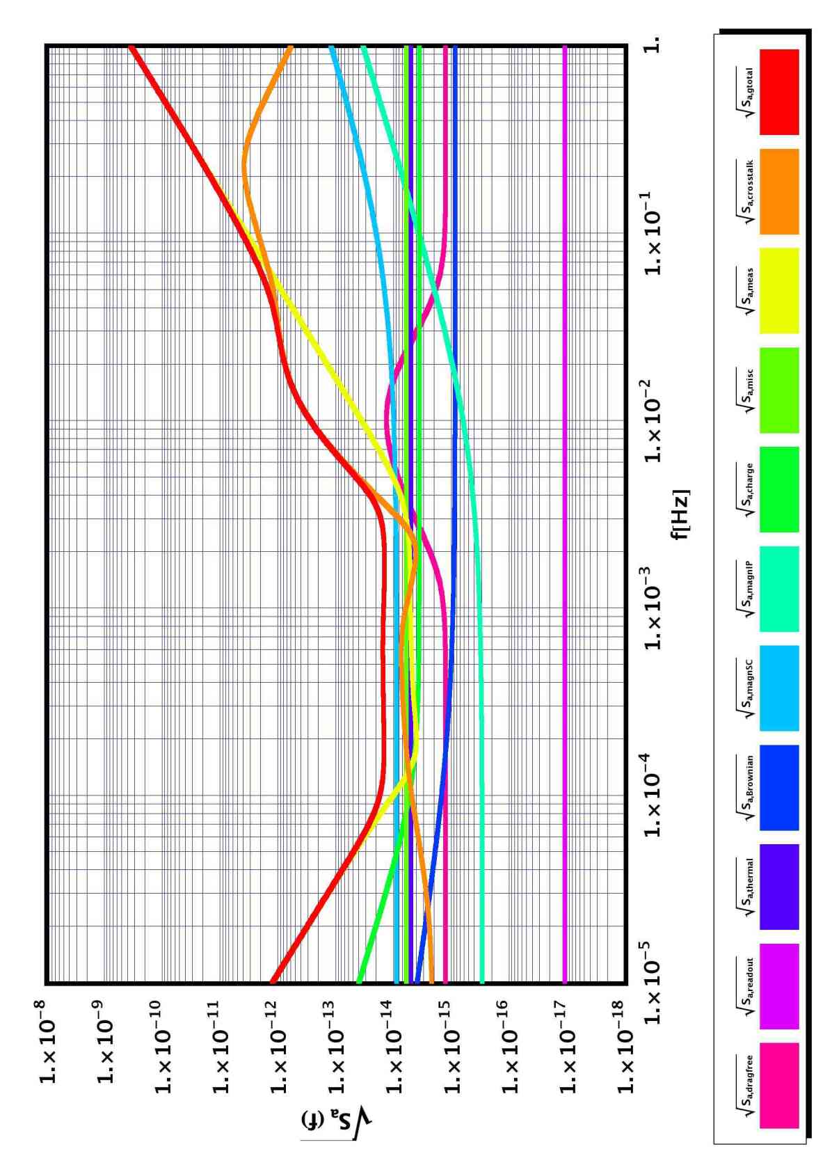
Figure 3.5: Graph of acceleration noise contributions. Grand total is in red.

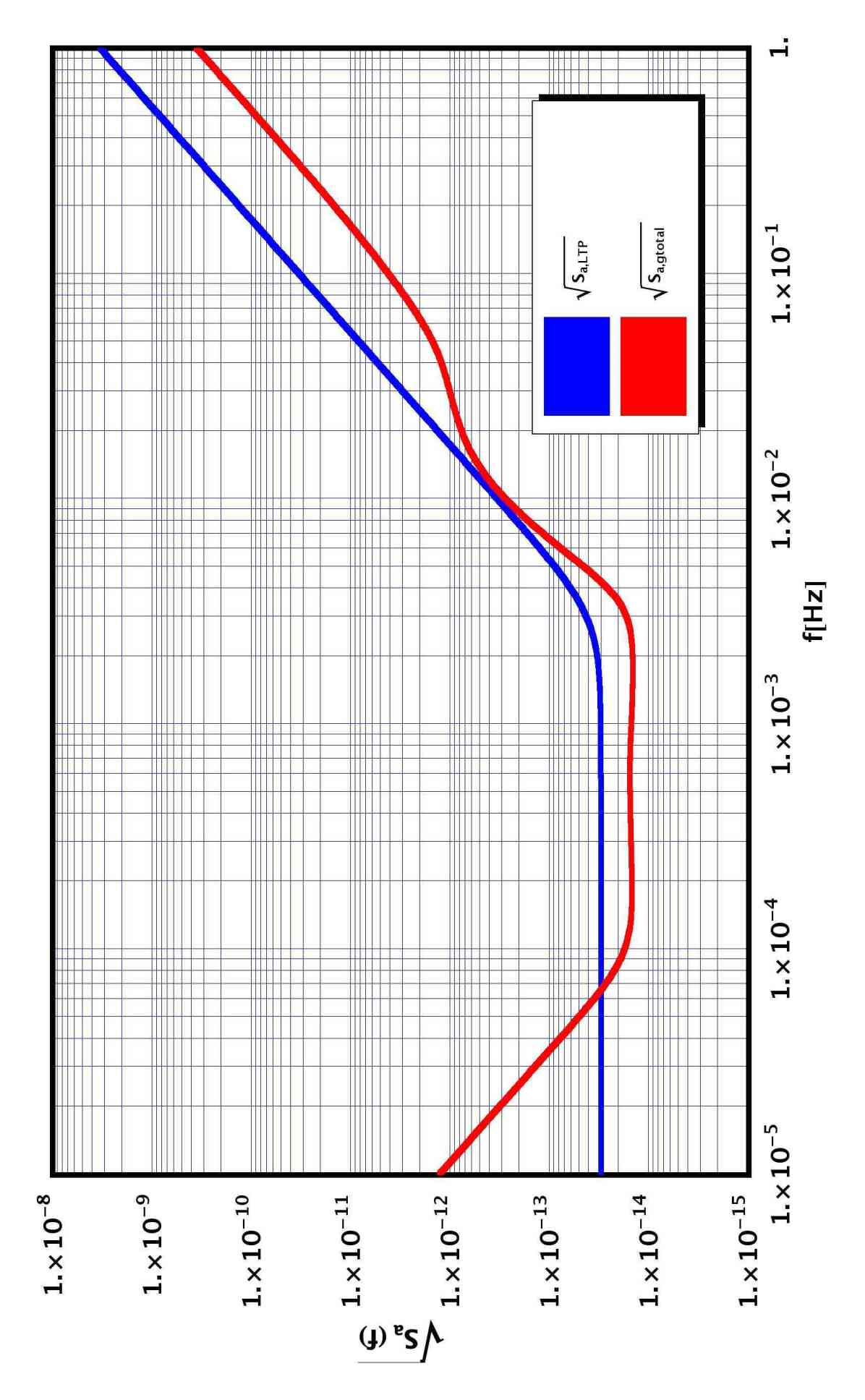
Figure 3.6: Grand total of acceleration noise (red) versus LTP requirement sensitivity curve (blue).

Chapter 4 Experiment and measures

We’d like to review here the experiment from a general side, pointing out the main experimental tasks, the sequence and priorities and a “run list”, providing a scheme of what will be the number of measures and describing them up to some extent.

LTP as a noise-probe facility embodies the main task of gaining knowledge of residual noise to model it in view of LISA. The chapter clarifies priorities in this perspective.

As a pre-requisite we’ll present two contributions: gravitational compensation and calibration of actuation forces.

The results will show that gravitational compensation can be achieved and it is robust against displacement and rotations. A discussion on meshing size, reliability and precision of estimates versus distance is sketched. Special attention was payed to engineering aspects, in view of the definition of a gravitational control protocol to discipline mass addition and removal from the SMART-2 satellite.

In the force calibration sections basic filter functions in somewhat simplified conditions will be sketched and the proper signals employed. Simplifications will not reduce the generality of the procedure or skip critical issues.

The optimal Kolmogorov filter theory will be used to retrieve a solution. The method provides a numeric pattern which can be convoluted with the detected data-set; moreover, the same procedure can be extended to many other analyses, as well as to similar problems on LISA.

Next, the run list gives insight to the different operations LTP will be asked to perform. This perspective shall show the reader how complicated and demanding the different tasks are and how important is therefore to get a clear noise picture reading as a first step, and then proceed with remaining tests.

We’ll present the measurement of the charge accumulated on the TMs to extend one of the main points in the “run list”. Such a feature is of paramount importance being a fundamental prerequisite for the GRS to operate properly. The measure will be carried on in science mode, continuously and compatibly with the science mode requirements; the same be valid for the discharge procedure. In view of optimising the detection different methods will be employed on purpose and estimates provided.

4.1 Main experimental task and phases

It became increasingly clear by inspecting LISA’s demands how important is to demonstrate that the acceleration requirement (1.65) is met when the TMs are used as fiducial mirrors for an interferometer based “local” metrology system [57, 58]. The importance of such a test is very high in view of localised measurements of TMs position relative to the OB placed in every LISA SC: the final displacement along one LISA’s arm is the sum of the optical signal (with baseline $5\times 10^{6}\,\mathrm{km}$) and two OB-to-TM signals, not to be underestimated in their precision. Thus, the displacement performance measurement at better than $10\,\nicefrac{\mathrm{pm}}{\mathrm{\sqrt{Hz}}}$, already included in LTP goals, has become a key science requirement.

LTP level of free-fall performance is set by worsening (1.72) [26] by a factor of $10$, and a term $\sqrt{2}$ appears since the measured acceleration will be differential and the residual forces on the test-masses are considered correlated over a short baseline:

$$S^{\nicefrac{{1}}{{2}}}_{\nicefrac{{\Delta F}}{{m}}}(\omega)=3\times 10^{-14}\left(1+\left(\frac{\omega}{2\pi\times 3\,\mathrm{mHz}}\right)^{4}\right)^{\nicefrac{{1}}{{2}}}\,\nicefrac{\mathrm{m}}{\mathrm{s^{2}\sqrt{Hz}}}\,,$$ (4.1)

however, the major data outcome of the SMART-2 mission will be the physical noise portrait for the quality of free-fall achievable on orbit around L1 within the limits of the same technology that will fly on LISA. Its analysis and crossing with the known noise models will produce a semi-empirical performance and disturbance model to build a realistic LISA sensitivity and environmental picture upon. The experience on ground-based interferometers is employed at this level for debugging and optimisation.

The general procedure calls for a detailed mathematical model in the frequency domain, and for the measurement of perturbation effects over the linear transfer functions upon application of distinct stimuli (magnetic fields or gradients, thermal gradients, electrostatic forces, variation in suspension gains, induced displacements) as functions of frequency. This allows to build up a deterministic map uniquely coupling sources and effects, other than “continuous” manifolds of parameters cross-correlations in seek for minimisation.

Optimal filtering theory is widely employed to produce discretised filters - by virtue of well-known models - to be convolved with the real stochastic data. This “noise projection” procedure provides thus a set of PSDs for all known sources, to be combined quadratically (assuming them to be uncorrelated) to hopefully explain the full acceleration and readout PSD curve, or to isolate unpredicted effects. Deviations between the semi-empirical model and the physical combined measurement upon projection are the hint of unfocused correlation and/or unpredicted noise and will demand further investigation.

In view of this scenario (which is physically very likely to occur), a line of priorities was drawn, a base schedule of measurements planned, and protocols written to support contingency on the formerly described events or in case of systems breakdown. The main experiment time-line is defined so to minimise the risk of missing the main science goals: a first noise portrait is taken as soon as minimal experimental conditions are met. Accuracy is improved as a second issue and calibrations come in the third place. Obviously measuring is a loop-wise procedure, the longer the experimental time and the more reliable the device proves to be, the highest the accuracy and more the pieces of physical information gathered.

Right after cruise phase (we assume all systems to be on-line from here) the first mission goal is obtaining a noise spectrum from the IFO and GRS signals even before TMs release. Environmental spectra will be taken together with the former ones. In the unfortunate possibility of Pathfinder systems failure, these valuable data will be a solid basis to check models and figures. We spare the reader of the technical details (see [57, 58]) and just state that “Basic Working Status” is reached when the TMs are floating and a reliable IFO signal providing the main relative TMs displacement ${\Delta}x$ is on-line.

Scan of the $1\,\mathrm{mHz}$ to $30\,\mathrm{mHz}$ (and beyond, if possible) frequency domain follows, book-keeping the $\text{IFO}({\Delta}x)$. We strongly point out that LTP will be the first space-borne mission to provide relative acceleration data at such a level of accuracy and precision, such a result would be a major advance in science in itself. A “Nominal Mode” (M1) measurement will be performed first, implying an easier control strategy and the self-calibration issues we discussed already. A “Science Mode” (M3) acceleration PSD measurement will follow, deemed to generate the first off-ground measurement of acceleration between two TMs in quasi-geodesic free-fall. To our best knowledge, this will be the most precise realisation of a TT-gauged laser-frequency-locked frame of reference.

4.1.1 Noise shooting and PSD minimisation phase

Once the goals of the former phases have been achieved, the next task is to minimise the PSD possibly to achieve the figure in (1.72) or beyond. Therefore the main sources of excess noise are identified and, whenever possible, minimised. The optimised noise PSD is then compared to the prediction obtained from the noise projections models.

All main diagnostics are at work and all data gathered simultaneously with the $\text{IFO}({\Delta}x)$ channel. This phase requires absolute calibration of acceleration [26] via the identification and suppression of anomalous physical disturbances and the identification and optimisation of anomalous direct and cross-coupling transfer functions from physical disturbances to the $\text{IFO}({\Delta}x)$ channel.

Dedicated experiments are planned on purpose:

Measurement and “diagonalising” of actuation

to displacement or rotation transfer functions. Large amplitude force and torque drives are applied to TM and SC measuring the outputs of all channels. By uploading several sets of parameters into the actuation matrix [41] and tracking the signals will result into a large sample of “reaction” matrices, to allow diagonalising the references and minimisation of cross-talk (see section 3.5.7 and [9, 12])

Measurement of the charge on test-mass

and subsequent discharging (non-continuous).

Identification of anomalous stray dc-voltages

on electrodes and their compensation by means of appropriate voltage biases.

Identification of anomalous magnetic noise

searching for anomalously large magnetic field and magnetic field gradient fluctuation from malfunctioning devices. The measurement of permanent magnetic moment of TM may take place to cross-check for variation after launch.

Identification of anomalous thermal effects

involves both temperature measurements and the measurement of the acceleration response to applied temperature gradients. Anomalous pressure and out-gassing phenomena may be identified.

Coarse measurement of stiffness

and stiffness matching.

Nominal and optimal values will be used to start the experimental phase and further optimised by variation of the most relevant (or suspected to be) ones. For example TMs position and orientation will be centred employing values from a-priori modelling, rotation jitter may be applied on a frequency span monitoring the $\text{IFO}({\Delta}x)$ output to estimate the “angular jitter to apparent displacement” effect as a function of frequency. The converse - displacing TM and reading angular jitter - gives the transposed cross-talk and both the transfer functions can be used to minimise the overall effect by redefining offsets or relative gains. To first order, cross-couplings may be assumed to be independent and evaluated with such procedures; fine-tuning multi-dimensional optimisation may be needed for higher-order corrections. Some effects may of course be thought as very weakly-coupled to some sources, e.g. the angular-linear jitter cross-talk is almost independent of temperature.

The system goes then into an iterative procedure where the previously estimated new optimal conditions become nominal values for the next loop, possibly improving the working point till maximum in matter of two-three loops. At every step comparison is made of the measured IFO PSD with the projected noise model, differences analysed and decisions taken on what to tune in the next step.

Ideally the achievement of the goal performance may put an even more stringent upper limit on any excess noise than the figure in (1.72); the computational accuracy of the noise model constitutes anyway a sort of default level, though the accuracy of the prediction of the noise floor depends critically on some system parameters to be measured like total magnetic field fluctuations, magnetic susceptibility, etc.

4.1.2 Noise model detailed investigation phase

A detailed investigation phase will begin right after cross-coupling optimisation has reached a reasonable convergence. In this new phase the LTP will be perform a dedicated set of experiments to “demonstrate” the noise model and allow further projection for LISA. The list of all planned measurements is discussed later [26].

The sequence of the “runs” is cast in logical priority list and tries to make best use of the given (and fore-casted) experimental time-span. Cross-coupling optimisation is repeated after more information on the noise contributions and parameters tweaking has been gathered thanks to the experiments sequence.

4.1.3 Extended investigation phase

Other key experiments that are part of the LISA Pathfinder mission are planned to take place in this phase. Specifically continuous charge measurements and continuous discharging will be performed, together with very long data runs to assess the performance of free fall and interferometry down to Fourier frequencies of $30\,\mathrm{{\mu}Hz}$, if possible, covering the full frequency range envisioned for LISA. On purpose, such data runs will have to extend over several days, to guarantee reliable data averaging as well.

A planned time slot should be reserved for this period for additional investigations that arise during the previous phases of the mission and are suggested by the science team and approved by the STOC.

This phase is called “extended” because it will add quite a deal of news to the former ones, but its priority is second with respect to taking a noise portrait and applying the noise projection scheme.

4.1.4 Fundamental science phase

During the Fundamental Science Phase, scientific investigations not directly addressing the verification of LISA technologies are performed. These investigations will have been suggested by the Science team during mission preparation. Examples could be investigations of Modified Newtonian Dynamics (MOND) theories, measurements of big-$G$, or a general validation of the inverse square law.

4.1.5 Extended mission phase

The need for more detailed investigations might have arisen during the nominal mission phase; these will be tackled in the Extended Mission Phase.

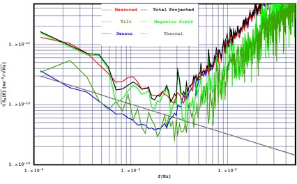
Figure 4.1: Data noise projection. The effect of measured magnetic field noise and apparatus tilt has been estimated from independent measurements and cross-spectra. Intrinsic thermal noise contribution has been calculated from measured pendulum properties. The black line is the sum of all expected contribution to total noise. Projection has been realised through the multi coherence method [13].

4.2 Fighting gravitational noise: compensation

4.2.1 Introduction

In the following we’ll name the three residual accelerations $\nicefrac{{{\boldsymbol{F}}}}{{m}}$, the three torques per unit moment of inertia $\nicefrac{{\gamma_{i}}}{{I_{i}}},\,i=1..3$ and the $6\times 6$ stiffness $\omega^{2}_{\text{p,grav},ij}$ “static gravitational imbalances” (SGI) since in our case they have gravitational nature and origin.

The SGI contribution to maximum acceleration and stiffness is significant: the total requirement for LTP is $\omega^{2}_{\text{p},\text{tot},xx}\leq 20\times 10^{-7}\,\mathrm{s}^{-2}@\,1\mathrm{mHz}$, while $\omega^{2}_{\text{p,grav},xx}\leq 5\times 10^{-7}\,\mathrm{s}^{-2}$ (see table 4.2 and [35]).

Why don’t we choose the easy way of electrostatic compensation? Dynamic compensation could be achieved by injecting DC voltage to produce a force by the GRS. But as it was shown in the noise chapter, any applied voltage produce a parasitic coupling in the form [36]:

$$\omega^{2}_{\text{p},\text{act},xx}=-\Delta a_{\text{DC}}\frac{\partial^{2}C_{x}}{\partial x^{2}}\left|\frac{\partial C_{x}}{\partial x}\right|^{-1}\,,$$ (4.2)

where $\Delta a_{\text{DC}}$ is the acceleration to counteract and we specialised the formula to the $\hat{x}$ direction of actuation (see (3.36)). $C_{x}$ is the actuators capacitance along $\hat{x}$. Moreover, "in band" fluctuation of the actuation drive voltage amplitude translate into acceleration noise, according to:

$$a_{\text{act},n}=2\Delta a_{\text{DC}}\cdot S^{\nicefrac{{1}}{{2}}}_{\nicefrac{{{\delta}V}}{{V_{\text{act}}}}}\,.$$ (4.3)

where $S^{\nicefrac{{1}}{{2}}}_{\nicefrac{{{\delta}V}}{{V_{\text{act}}}}}$ is the noise spectral density of the actuation voltage. Both the stiffness and actuation force noise are thus proportional to the residual imbalanced $\Delta a_{\text{DC}}$.

Static compensation of gravity imbalance is thus mandatory to reduce budget on the amount of static parasitic stiffness and to lower the related acceleration noise. In this scenario, maximal budgets have been assigned to each stiffness and noise contribution. The maximal SGI and can be found in tables 4.1 and 4.2.

In principle, perfect compensation to annihilate all the SGI might be possible, but given the set of requirements, we need only to find the minimum mass distribution, with best geometry to bring the SGI values within requirement. Due to engineering needs, these compensation masses (CmpMs) shall be easy to manufacture and mount and, additionally, should be geometrically as simple as possible.

$\nicefrac{{\Delta F_{x}}}{{m}}$		$\nicefrac{{\Delta F_{y}}}{{m}}$		$\nicefrac{{\Delta F_{z}}}{{m}}$		$\nicefrac{{\gamma_{\theta}}}{{I_{\theta}}}$		$\nicefrac{{\gamma_{\eta}}}{{I_{\eta}}}$		$\nicefrac{{\gamma_{\phi}}}{{I_{\phi}}}$
$1$	$.1$	$1$	$.7$	$3$	$.2$	$14$	$.0$	$18$	$.0$	$23$	$.0$

Table 4.1: Requirements on forces and torques, TM1-TM2 (forces), TM1 only (torques). Absolute values. $F_{i}/m$ in $[\mathrm{nm\,s}^{-2}]$, $T_{i}/I_{i}$ in $[\mathrm{nrad\,s}^{-2}]$ for each $i$.

	$\nicefrac{{F_{x}}}{{m}}$		$\nicefrac{{F_{y}}}{{m}}$		$\nicefrac{{F_{z}}}{{m}}$		$\nicefrac{{\gamma_{\theta}}}{{I_{\theta}}}$		$\nicefrac{{\gamma_{\eta}}}{{I_{\eta}}}$		$\nicefrac{{\gamma_{\phi}}}{{I_{\phi}}}$
${{\partial}_{x}}$	$500$	$.0$	$7$	$.0$	$7$	$.0$	$-$		$-$		$-$
${{\partial}_{y}}$	$7$	$.0$	$500$	$.0$	$-$		$-$		$-$		$-$
${{\partial}_{z}}$	$7$	$.0$	$-$		$1000$	$.0$	$-$		$-$		$-$
${{\partial}_{\theta}}$	$14$	$.0$	$-$		$-$		$1960$	$.0$	$-$		$-$
${{\partial}_{\eta}}$	$14$	$.0$	$-$		$-$		$-$		$1960$	$.0$	$-$
${{\partial}_{\phi}}$	$14$	$.0$	$-$		$-$		$-$		$-$		$1480$	$.0$

Table 4.2: Requirement on stiffness, linear-angular and angular-angular gradients over TM1. Absolute values. Dimensions for each element are $10^{-9}[\mathrm{s}^{-2}]$. The symbol “$-$” means no precise requirement is demanded.

We refer now to the system of coordinates in figure 4.2, left. The gravitational force along the $i$-th axis, exerted by a material point with mass $m$ located on ${\boldsymbol{r}}=\left\{x,y,z\right\}$ on the homogeneous TM with mass $m$ and volume $V=L_{x}L_{y}L_{z}$ whose centre of mass is chosen as the origin of coordinates, can be analytically calculated as the integral of the usual Newtonian potential [59, 8]: $\Phi(x,y,z)=\nicefrac{{Gm}}{{\left|{\boldsymbol{r}}\right|}}$. Torques follow from the definition: ${\boldsymbol{\gamma}}={\boldsymbol{r}}\wedge{\boldsymbol{F}}=\left\{\gamma_{\theta},\gamma_{\eta},\gamma_{\phi}\right\}$, while the linear stiffness matrix can be computed by means of $\omega^{2}_{\text{p,grav},ij}({\boldsymbol{r}})=\partial_{i}F_{j}({\boldsymbol{r}})$. Ancillary formulae must be employed to compute angular-linear, angular-angular gradients due to the spatial extent of the TMs. For example, to calculate the derivative of the force with respect to the angular DOF conjugated to $\hat{z}$, i.e. $\hat{\phi}$, we would use:

$$\partial_{\hat{\phi}}{\boldsymbol{F}}=(\hat{\phi}\wedge{\boldsymbol{F}})-\left((\hat{\phi}\wedge{\boldsymbol{r}})\cdot{\boldsymbol{\nabla}}_{r}\right){\boldsymbol{F}}\,.$$ (4.4)

In this way, we are left with only translational derivatives to compute. For example:

$$\omega^{2}_{\text{p,grav},\phi x} =\frac{\partial F_{x}}{\partial\phi}=\frac{\partial\gamma_{\phi}}{\partial x}=-F_{y}-x\omega^{2}_{\text{p,grav},xy}+y\omega^{2}_{\text{p,grav},xx}\,,$$ (4.5)

$$\omega^{2}_{\text{p,grav},\phi\theta} =\frac{\partial\gamma_{\theta}}{\partial\phi}=xF_{x}+yF_{y}-y^{2}\omega^{2}_{\text{p,grav},xx}-x^{2}\omega^{2}_{\text{p,grav},yy}-2xy\omega^{2}_{\text{p,grav},xy}\,,$$ (4.6)

where we implied $F_{i}=F_{i}({\boldsymbol{r}})$, $\gamma_{i}=\gamma_{i}({\boldsymbol{r}})$, $\omega^{2}_{\text{p,grav},ij}=\omega^{2}_{\text{p,grav},ij}({\boldsymbol{r}})$ for any $i,j$.

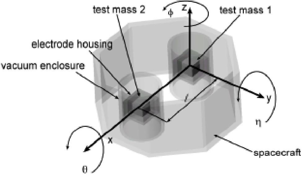
Figure 4.2: On the left: reference system of the LTP. Schematic view of the experimental apparatus’s of the LTP with the main DOF of the freely floating TM. On the right: top-side view of the available room inside the vacuum enclosure hosting each TM (see [14, 8]).

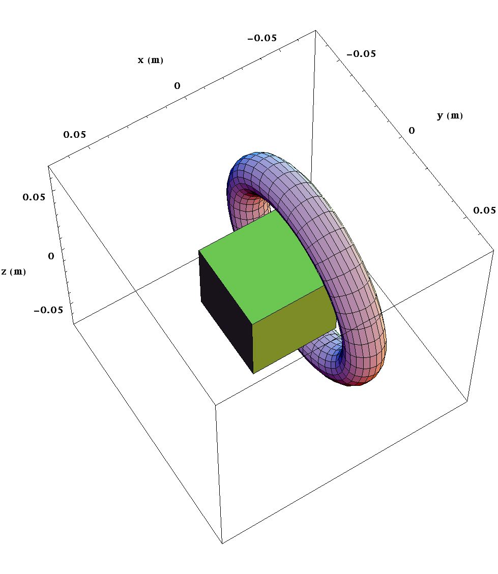
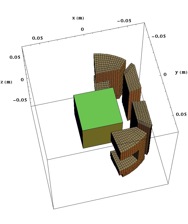
Figure 4.3: Left: tentative shape of compensating ring contributing positive gravitational stiffness. On the right: final shape of compensation masses (4 lobes) around TM1.

4.2.2 Explaining the strategy

The SGI due to the different components on board (DRS, LTP, SC) have been evaluated by means of (4.5), (4.6) and similar formulae, after meshing of each structure. A dedicated Mathematica®  code was written to mesh simple polyhedron’s forms as well as reading nodes-elements STEP files, allowing computation of forces, torques and derivatives from point-like sources on a generic cubic mass.

Meshing was chosen to be adaptive, tetrahedral, with size $\sim 2\,\mathrm{mm}$ maximum, while the density and mass distribution of the sub-components is known for each subsystems. The mesh size is chosen for the different masses as a function of distance and object size in order to obtain the required precision and is a compromise with computational time and power constraints. We note that $2\leavevmode\nobreak\ \mathrm{mm}$ size is a conservative choice for nearby IS and OB hardware and could be relaxed for more distant spacecraft components (see beyond for a more complete discussion and formulae).

Contributions coming from different blocks vary in their relevance; linearity of the SGIs permits us to sum the contributions to the total SGIs, taking advantage of symmetries and partial cancellations. Resulting values can be found in tables 4.3 and 4.4. Notice the accelerations $\nicefrac{{\Delta F_{x}}}{{m}}$, $\nicefrac{{\Delta F_{y}}}{{m}}$, $\nicefrac{{\Delta F_{z}}}{{m}}$ are differential, because only the relative acceleration counts for these DOF on LTP. On the other hand torques and stiffness are computed with absolute reference to TM1.

After receiving input on boundary conditions and limits, the code performs a weighted choice of the allowed elements in free space thus giving the sum of the related contributions. The weighing is optimised to completely eliminate $\Delta F_{x}$ while minimising stiffness. Once a solution is found, it may be refined at will, by re-meshing and re-weighing.

Notice from tables 4.3 and 4.4 that the uncompensated value of $\nicefrac{{\Delta F_{x}}}{{m}}$ is $60$ times larger than the allowed value; the other values of the force-torques vector appear to be within requirements. The same for the stiffness matrix, showing a small, negative spring for $\omega^{2}_{\text{p,grav},xx}$ and a value of $\omega^{2}_{\text{p,grav},\eta x}$ just the $3\%$ out of specification.

The positions of the two CmpMs are chosen to minimise the distance to the TMs, to achieve maximum effect for a given mass (forces scale like $\nicefrac{{1}}{{r^{2}}}$, $r$ mutual distance between the bodies). The largest contiguous portion of available free room around each TMs between the electrode housing (EH) and vacuum enclosure (VE) has been considered a suitable location for the CmpMs (see figure 4.2, right) and reduced to geometrically simple elements for meshing.

The CmpMs are then assumed to be in Tungsten, due to its high density ($19300\,\nicefrac{\mathrm{kg}}{\mathrm{m^{3}}}$) and modelled assuming the TMs in centred, nominal position.

The tentative ideal shape of a torus, coaxial with the LTP $\hat{x}$ axis, belt-like around each TMs had been chosen. The far ring used for compensating will look like a point as seen from each far TM, while it is a true torus for the closer TM. The rings thus attract the TMs outwards, compensating $\Delta F_{x}$ without introducing undesirable $\hat{x}$-gradient stiffness due to the rotational symmetry of the tori (of course this is not the case for $\hat{y}$, $\hat{z}$). This analysis on springs constants accounts for the gravitational budget; electrostatic negative stiffness will still dominate the scenario, but pure gravitational springs induced by this configuration are positive nevertheless.

A picture of the starting shape can be seen in figure 4.3, left. Due to lack of space on the upper and lower parts, each perfect ring gets cut into two lobes, enlarged toward the $\hat{x}$ axis to embed each TM. The CmpMs assume the final form of eight lobes, four on each TM, standing on the external side of the cubes (see figure 4.3, right), between the VE and EH. Each CmpMs weights $2.51\pm 0.04\,\mathrm{kg}$. Resulting residual value in $\nicefrac{\mathrm{\Delta F_{x}}}{\mathrm{m}}$ is highly sensitive to the CmpMs mass: the imbalance in $\nicefrac{\mathrm{\Delta F_{x}}}{\mathrm{m}}$ cannot be compensated with a smaller mass.

The CmpMs gravitational contribution brings the overall SGI values within requirements as shown in tables 4.5 and 4.6 in comparison with tables 4.1 and 4.2. We note in comparing tables 4.5 and 4.3 that we have successfully compensated $\nicefrac{{\Delta F_{x}}}{{m}}$ without significantly disturbing the other forces and torques, which were already compliant with the requirements even before compensation. Unfortunately this is obtained with the price of a considerable increase in $\omega^{2}_{\text{p,grav},xx},\omega^{2}_{\text{p,grav},yy},\omega^{2}_{\text{p,grav},zz}$ and other DOF in table 4.6. The $\omega^{2}_{\text{p,grav},xx}$ factor is a negative stiffness close in value to the requirement limit, although this proves to be still reasonable for LTP [35]. Conversely, the $\omega^{2}_{\text{p,grav},zz}$ factor looks like a positive spring, increasing robustness in $\hat{z}$.

$\nicefrac{{\Delta F_{x}}}{{m}}$		$\nicefrac{{\Delta F_{y}}}{{m}}$		$\nicefrac{{\Delta F_{z}}}{{m}}$		$\nicefrac{{\gamma_{\theta}}}{{I_{\theta}}}$		$\nicefrac{{\gamma_{\eta}}}{{I_{\eta}}}$		$\nicefrac{{\gamma_{\phi}}}{{I_{\phi}}}$
$65$	$.7$	$-0$	$.13$	$0$	$.58$	$0$	$.04$	$0$	$.36$	$0$	$.05$

Table 4.3: Forces and Torques exerted by the SC, DRS and LTP Path-finder systems over TM1-TM2 (forces) and TM1 only (torques). $F_{i}/m$ in $[\mathrm{nm\,s}^{-2}]$, $T_{i}/I_{i}$ in $[\mathrm{nrad\,s}^{-2}]$ for each $i$.

	$\nicefrac{{F_{x}}}{{m}}$		$\nicefrac{{F_{y}}}{{m}}$		$\nicefrac{{F_{z}}}{{m}}$		$\nicefrac{{\gamma_{\theta}}}{{I_{\theta}}}$		$\nicefrac{{\gamma_{\eta}}}{{I_{\eta}}}$		$\nicefrac{{\gamma_{\phi}}}{{I_{\phi}}}$
${{\partial}_{x}}$	$38$	$.57$	$4$	$.83$	$-0$	$.87$	$-7$	$.02$	$-39$	$.29$	$5$	$.13$
${{\partial}_{y}}$	$4$	$.84$	$-23$	$.88$	$-5$	$.62$	$137$	$.17$	$2$	$.45$	$17$	$.67$
${{\partial}_{z}}$	$-0$	$.88$	$-5$	$.64$	$-14$	$.7$	$11$	$.53$	$18$	$.87$	$4$	$.56$
${{\partial}_{\theta}}$	$-0$	$.01$	$14$	$.45$	$-0$	$.1$	$31$	$.42$	$-1$	$.16$	$2$	$.93$
${{\partial}_{\eta}}$	$-14$	$.43$	$0$	$.0$	$-61$	$.82$	$-1$	$.1$	$33$	$.31$	$0$	$.28$
${{\partial}_{\phi}}$	$0$	$.1$	$61$	$.82$	$0$	$.0$	$2$	$.57$	$0$	$.33$	$26$	$.41$

Table 4.4: Stiffness, linear-angular and angular-angular gradients exerted by the SC, DRS and LTP Path-finder systems over TM1. Dimensions for each element are $10^{-9}[\mathrm{s}^{-2}]$.

$\nicefrac{{\Delta F_{x}}}{{m}}$		$\nicefrac{{\Delta F_{y}}}{{m}}$		$\nicefrac{{\Delta F_{z}}}{{m}}$		$\nicefrac{{\gamma_{\theta}}}{{I_{\theta}}}$		$\nicefrac{{\gamma_{\eta}}}{{I_{\eta}}}$		$\nicefrac{{\gamma_{\phi}}}{{I_{\phi}}}$
$-0$	$.05$	$-0$	$.13$	$0$	$.58$	$0$	$.05$	$0$	$.49$	$0$	$.08$

Table 4.5: Residual forces and torques on TM1-TM2 (forces) and TM1 only (torques). $F_{i}/m$ in $[\mathrm{nm\,s}^{-2}]$, $T_{i}/I_{i}$ in $[\mathrm{nrad\,s}^{-2}]$ for each $i$.

	$\nicefrac{{F_{x}}}{{m}}$		$\nicefrac{{F_{y}}}{{m}}$		$\nicefrac{{F_{z}}}{{m}}$		$\nicefrac{{\gamma_{\theta}}}{{I_{\theta}}}$		$\nicefrac{{\gamma_{\eta}}}{{I_{\eta}}}$		$\nicefrac{{\gamma_{\phi}}}{{I_{\phi}}}$
${{\partial}_{x}}$	$471$	$.61$	$5$	$.09$	$-3$	$.63$	$-6$	$.91$	$-31$	$.67$	$3$	$.96$
${{\partial}_{y}}$	$5$	$.1$	$161$	$.37$	$-5$	$.69$	$140$	$.49$	$2$	$.0$	$-697$	$.89$
${{\partial}_{z}}$	$-3$	$.64$	$-5$	$.71$	$-632$	$.99$	$10$	$.88$	$61$	$.83$	$4$	$.9$
${{\partial}_{\theta}}$	$-0$	$.01$	$13$	$.95$	$-0$	$.13$	$5$	$.34$	$-1$	$.2$	$2$	$.65$
${{\partial}_{\eta}}$	$-13$	$.93$	$0$	$.0$	$3$	$.67$	$-1$	$.11$	$88$	$.92$	$0$	$.29$
${{\partial}_{\phi}}$	$0$	$.13$	$-3$	$.91$	$0$	$.0$	$2$	$.16$	$0$	$.34$	$-2$	$.09$

Table 4.6: Residual stiffness, linear-angular and angular-angular gradients over TM1. Dimensions for each element are $10^{-9}[\mathrm{s}^{-2}]$.

4.2.3 Robustness and tests

Several aspects of this strategy need to be clarified:

• the dependence of the SGI on the source knowledge (shape, position and density) needs further investigation to render our results robust against small mass variation (due to assembly imprecision or design changes) at a given distance. The definition of a “gravitational protocol” to discipline mass addition/removal from the Path-finder systems is in advanced progress [8]. In our analysis we crudely assumed precise knowledge of the positioning of the subsystems blocks as well as their density;

• inhomogeneity of the TMs has not been investigated, although such a scenario may be mapped into a suitable point-like mass distribution in the proximity of each TM generating an effective field to mimic bubbles, cracks and surface defects. Nonetheless, in the present work we assumed perfect cubic TMs;

• the compensation reliability depends on the knowledge of the CmpMs mass, shape and positioning. Therefore we performed tests to shed light on uncertainties in the meshing procedure as well as in the placement upon translations and rotations.

4.2.3.1 Rotations and translations

We displaced CmpM1 by roto-translating it, while CmpM2 was assumed to be perfectly placed. Residual SGIs remain within specifications under small rotations but become less robust in the process until exceeding the allowed values for rotations with Euler angles $(\eta,\theta,\phi)\leavevmode\nobreak\ >\leavevmode\nobreak\ 3\times\leavevmode\nobreak\ 10^{-3}\,\mathrm{rad}$. Stiffness begins to exceed first along the $xy$, $yz$ couples. The uncertainty in rotation upon placement of the CmpMs can be checked by measuring the position of the CmpMs sides and shall not exceed the nominal position more than $300\,\mathrm{\mu m}=3\cdot 10^{-3}\,\mathrm{rad}\cdot R_{VE}$, with $R_{VE}=10\,\mathrm{cm}$ being the radius of the VE chamber.

The analysis on translations is similar to the one carried out for rotations. By moving CmpM1 with a vector whose maximum length is $\sim 300\,\mathrm{\mu{m}}$, predominantly in the sensitive $\hat{x}$ direction, parameters are seen to be within specifications. Larger translation induce breakdown either along cross directions (translations with dominant off-$\hat{x}$ terms) or along the $\hat{x}$ direction of the force.

4.2.3.2 Density and meshing, placing

Since Tungsten cannot be easily purified beyond $95\%$ of the nominal density, we assumed a $5\%$ error on density during simulation, mimicking impurities and defect in production using an isotropic bubble distribution in the mesh. Provided the mass is $2.51\pm 0.04\,\mathrm{kg}$ per CmpMs, compensation can be achieved in spite of the defects. Of course, a larger volume is needed to reach the mass demand.

To circumvent potential problems of density inhomogeneity, the CmpMs can be over-sized at first and then trimmed to the appropriate weight. Maximum needed over-sizing is estimated to be around $2-3\,\mathrm{mm}$ which compensates for the $5\%$ mass defect; recommended growing points are the “back” and side “wings” of the CmpMs (see figure 4.3, right).

Additional checks on the ideal mesh element size have been performed. Each mesh brick field is the result of an average of $\leavevmode\nobreak\ 1000$ sub-bricks. This way the size of $\sim 2\,\mathrm{mm}$ proves to be sufficiently fine for the purpose of our analysis. Mass loss due to meshing of the volumes is under control and doesn’t contribute more than $0.1\%$ of the calculated field values.

Generally speaking, both the problems of meshing and misplacement upon mounting can be addressed analytically. Ordinary meshing software doesn’t encounter any trouble when dealing with straight corners and sharp surfaces, problems arise when curvature is at work: adherence to a curved bounding manifold when mapping its volume with meshing bricks is necessarily approximated. We can model it as follows: choose tetrahedrons as bricks and a sphere as the target object. The inner volume of the sphere will not bring any trouble, even cubes could map it correctly up to the surface. The number of external tetrahedrons adhering to the surface is roughly given (no combinatorial) by the ratio of the sphere surface measure and tetrahedrons base area:

$$N\simeq\frac{4\pi R^{2}}{\frac{\sqrt{3}}{4}L^{2}}\,,$$ (4.7)

where we named $R$ the sphere radius and $L$ the tetrahedron side. In fact, more care should be placed into combining the shapes on the surface and the integer value of the former must be taken, but to zero-order the former is not wrong.

We may then assume each tetrahedron to extend till the sphere centre therefore becoming a pyramid whose long side be $R$; the height can then be computed as:

$$h=\sqrt{R^{2}-\left(\frac{2}{3}\frac{\sqrt{3}}{2}L\right)^{2}}\,,$$ (4.8)

and the volume as:

$$V=\frac{1}{3}h\frac{\sqrt{3}}{4}L^{2}\,.$$ (4.9)

The relative meshing error is the difference in volume from real to estimated divided by the real one itself:

$$\epsilon_{\text{mesh}}=\frac{\frac{4}{3}\pi R^{3}-NV}{\frac{4}{3}\pi R^{3}}=1-\sqrt{1-\frac{1}{3}\left(\frac{L}{R}\right)^{2}}\,,$$ (4.10)

as expected, the former goes to $0$ as $L\ll R$, and to first order in $\nicefrac{{L}}{{R}}$ we get:

$$\epsilon_{\text{mesh}}=\frac{1}{6}\left(\frac{L}{R}\right)^{2}+O\left(\left(\frac{L}{R}\right)^{2}\right)\,.$$ (4.11)

On the other hand the misplacement error can be computed from the expression of the force. In modulus:

$$F=G\frac{m_{1}m_{2}}{r^{2}}\,,$$ (4.12)

we have

$$\delta{F}=-2G\frac{m_{1}m_{2}}{r^{3}}\delta{r}\,,$$ (4.13)

and

$$\epsilon_{F}=\left|\frac{\delta{F}}{F}\right|=2\frac{\delta{r}}{r}\,.$$ (4.14)

Henceforth, the former representing the relative error on force upon displacement - undesired or not - it also describes the dependence of the meshing length scale with respect of the distance scale from the observer to confine force estimate error to a given value $\epsilon_{F}$. Formula (4.10) together with (4.14) are powerful tool to estimate the minimal side of meshing brick and the relevance of mass addiction according to distance from the TMs.

4.2.4 Open issues. Gravitational control protocol

The results show that the SGI can be compensated within the required levels. At the end of this investigation, while masses, shapes and sizes appear to be reasonable, a number of engineering challenges remain: machinability and trimming, compatibility with both the mass and position of cabling, and mounting procedures.

The calculation presented here is the first step toward assessing if the following gravitational compensation protocol may be followed:

1. based on nominal design of SC, LTP and DRS, calculation of the gravitational disturbances on the test-mass is performed and a first design of compensation masses is provided. This design allows the preliminary definition of the mechanical interfaces of the compensation masses and to tackle the interference problems;

2. at Critical Design Review (CDR), based on the available design knowledge of SC and LTP, the design of interference-avoidance features and of mechanical interfaces is frozen;

3. a Gravitational System Review (GSR) is introduced within the planning to freeze the final trimming of the compensation mass design. This final trimming can only relate to minor adjustments of the outer surfaces of compensation masses and cannot affect their mechanical interfaces. A change of these would indeed imply a redesign of the entire inertial sensor;

4. after GSR final manufacturing of compensation masses is performed. From there on compensation must be performed by masses outside the VE and a specific mechanical interface for that must be designed.

4.3 Calibrating force to displacement

4.3.1 Calibration of force applied to TM1

In order to calibrate the force applied to the first TM, expressed by the term $g_{1,x}$ in (2.114), (2.131) and derived ones, the most convenient signal to employ is in fact (2.131). By setting to $0$ all the spare contribution but for $g_{1,x}$, we see the signal equation reduces to:

$$\text{IFO}\left(x_{1}\right)\simeq h_{x,x_{1},x_{1}}(s)g_{1,x}=\frac{1}{s^{2}+\omega_{\text{df},x_{1}}^{2}+\omega_{x_{1},x_{1}}^{2}}\,.$$ (4.15)

Where all the terms have been discussed in chapter 2. The former equation neglects the need for any calibration, a thing we know for sure to be false. Had we to complicate the model so to introduce a bona-fide mimicking of this unbalance, a proportionality factor $\kappa_{\text{TM1}}$ would appear homogeneous to $h_{x,x_{1},x_{1}}$ but would also be placed to multiply $\omega_{\text{df},x_{1}}^{2}$ since the drag-free control loop makes use of the same readout apparatus to exert force, hence suffering the same lack of calibration. Moreover, we can’t assume anymore the full stiffness to be given by $\omega_{x_{1},x_{1}}^{2}$ only, we’ll hence replace the factor with a generic $\tilde{\omega}_{x_{1},x_{1}}^{2}$.

Expression (4.15) gets thus modified and displays like:

$$\text{IFO}\left(x_{1}\right)\simeq\frac{\kappa_{\text{TM1}}}{s^{2}+\kappa_{\text{TM1}}\omega_{\text{df},x_{1}}^{2}+\tilde{\omega}_{x_{1},x_{1}}^{2}}g_{1,x}\,.$$ (4.16)

We proceed to linearised the problem by introducing the following approximations:

$$\begin{split}\tilde{\omega}_{x_{1},x_{1}}^{2}&\simeq\omega_{x_{1},x_{1}}^{2}+{\delta}k_{1}\,,\\ \kappa_{\text{TM1}}&\simeq 1+{\delta}k_{2}\,,\end{split}$$ (4.17)

where obviously ${\delta}k_{2}\ll 1$ and ${\delta}k_{1}\ll\omega_{\text{df},x}^{2}$ together with ${\delta}k_{1}\ll\omega^{2}=-s^{2}$. By expanding (4.16) to first order in ${\delta}k_{2}$ and ${\delta}k_{1}$ we find:

$$\text{IFO}\left(x_{1}\right)\simeq f_{0}(s)+f_{1}(s)+f_{2}(s)\,,$$ (4.18)

where

$$\begin{split}f_{0}(s)&=H_{0}(s)g_{1,x}\,,\\ f_{1}(s)&=H_{0}(s)H_{1}(s){\delta}k_{1}g_{1,x}\,,\\ f_{2}(s)&=H_{0}(s)H_{2}(s){\delta}k_{2}g_{1,x}\,,\end{split}$$ (4.19)

and where

$$H_{0}(s) \doteq h_{x,x_{1},x_{1}}(s)\,,$$ (4.20)

$$H_{1}(s) \doteq-h_{x,x_{1},x_{1}}(s)\,,$$ (4.21)

$$H_{2}(s) \doteq 1-h_{x,x_{1},x_{1}}(s)\omega^{2}_{\text{df},x_{1}}\,,$$ (4.22)

The first component, $f_{0}$, represents the ideal signal, that would be measured under perfect calibration and accuracy conditions; the latter two, $f_{1}$ and $f_{2}$ are due to parasitic stiffness and non-ideal conversion from actuation command and real effect on the TM1. This way the transfer function is written in a form suitable for the application of the optimal filter theory:

$$x=g_{1,x}H_{0}(s)\left(1+{\delta}k_{1}H_{1}(s)+{\delta}k_{2}H_{2}(s)\right)\,.$$ (4.23)

According to the Wiener-Kolmogorov optimal filter theory, a set of coefficients ${\delta}k_{i}\,,\,i=1,2$ in a signal of the form

$$x(t)=n(t)+A_{0}\left(f_{0}(t)+{\delta}k_{1}f_{1}(t)+{\delta}k_{2}f_{2}(t)\right)\,,$$ (4.24)

may be estimated linearly up to optimal precision as follows. By subtracting the predictable $0$ component, we introduce the deviation:

$$\tilde{x}(t)\doteq x(t)-A_{0}f_{0}(t)\,,$$ (4.25)

and the linear combinations

$$\hat{A}_{i}\doteq\int_{\mathbb{R}}h_{i}(\tau)\tilde{x}(\tau)\operatorname{d}\tau\,$$ (4.26)

defined so that the average values are homogeneous in the deviation coefficients:

$$\left\langle\hat{A}_{i}\right\rangle=A_{0}{\delta}k_{i}\,.$$ (4.27)

The $h_{i}(\tau)$ filter transfer functions are designed to minimise the root mean square errors of the estimates, as follows:

$$\sigma^{2}_{\hat{A}_{i}}\doteq\int_{{\mathbb{R}}^{2}}h_{i}(\tau^{\prime})h_{i}(\tau^{\prime\prime})C(\tau^{\prime}-\tau^{\prime\prime})\operatorname{d}\tau^{\prime}\operatorname{d}\tau^{\prime\prime}\,,$$ (4.28)

where $C(\tau)$ is the auto-correlation function already defined in chapter 1, linked to the PSD $S(\omega)$ by the Fourier anti-transform (see (1.43) and (1.44)). No summation is implied in the former equation. By Lagrange multipliers maximisation of (4.28) under the bonds (4.27) the solution is found for the $h_{i}$ functions as

$$h_{i}(\omega)=\frac{1}{S(\omega)}\sum_{j}\Lambda_{ij}f_{j}(\omega)\,,$$ (4.29)

where $\Lambda$ is the covariance matrix associated to the optimal solution:

$$\Lambda_{ij}=\left\langle\hat{A}_{i}\hat{A}_{j}\right\rangle\,,$$ (4.30)

defined as

$$\Lambda_{ij}^{-1}\doteq\frac{1}{2\pi}\int_{\mathbb{R}}\frac{f_{i}(\omega)f_{j}^{*}(\omega)}{S(\omega)}\operatorname{d}\omega\,.$$ (4.31)

The covariance matrix for ${\delta}k_{1}$ and ${\delta}k_{2}$ is thus:

$$\Lambda=A_{0}^{2}\left[\begin{array}[]{cc}\sigma^{2}_{{\delta}k_{2}}&r\sigma_{{\delta}k_{2}}\sigma_{{\delta}k_{1}}\\ r\sigma_{{\delta}k_{2}}\sigma_{{\delta}k_{1}}&\sigma^{2}_{{\delta}k_{1}}\end{array}\right]\,,$$ (4.32)

where we introduced the variances for ${\delta}k_{i}\,,\,i=1,2$ and their correlation coefficient $r$.

We now apply the optimal filter theory to the formerly defined expressions for $f_{i}$, expressions (4.19). We get for the covariance matrix that:

$$\Lambda=\left[\frac{1}{2\pi}\int_{\mathbb{R}}H_{i}(\omega)H_{j}^{*}(\omega)\frac{\left|g_{1,x}(\omega)\right|^{2}}{S_{g}(\omega)}\operatorname{d}\omega\right]^{-1}\,,$$ (4.33)

where

$$\begin{split}S_{g}(\omega)\doteq\frac{S(\omega)}{\left|H_{0}(\omega)\right|^{2}}=&\left(3\times 10^{-14}\right)^{2}\nicefrac{\mathrm{m^{2}}}{\mathrm{s^{4}Hz}}\left(1+\left(\frac{2\pi\times 0.9}{\omega\nicefrac{{1}}{{\mathrm{mHz}}}}\right)^{6}\right)\\ &+\left(9\times 10^{-12}\right)^{2}\nicefrac{\mathrm{m^{2}}}{\mathrm{Hz}}\left(\omega^{2}+\tilde{\omega}_{x_{1},x_{1}}^{2}\right)^{2}\,.\end{split}$$ (4.34)

Such a choice depends on the performance of the interferometer ($9\,\nicefrac{{\mathrm{pm}}}{{\sqrt{\mathrm{Hz}}}}$) and on the requirement on acceleration noise ($3\times 10^{-14}\,\nicefrac{{\mathrm{m}}}{{\mathrm{s^{2}}\sqrt{\mathrm{Hz}}}}$); the noise in acceleration worsens rapidly below $1\,\mathrm{mHz}$ as a function of $\left(\nicefrac{{\omega}}{{2\pi}}\right)^{-6}$. A graph may be viewed in picture 4.4.

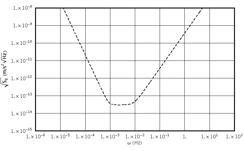
Figure 4.4: Root squared PSD for $S_{g}(\omega)$.

The calibration signal used for calibration “in silico” would be a bi-damped cosine with frequency $\nu_{0}$ and characteristic damping time $\tau$:

$$g(t)=\exp\left(-\frac{\left|t\right|}{\tau}\right)\cos 2\pi\nu_{0}t\,.$$ (4.35)

The functional behaviour of $\omega_{\text{df},x_{1}}^{2}$ can be read out of (2.145) together with table 2.5.

Finally, $A_{0}$ was chosen so to avoid saturation and retain linearity in the signal response. Practically, this corresponds to the introduction of two joined conditions:

$$\left|A_{0}f_{0}(t)\right|\leq 0.1\,\mathrm{\mu m}\quad\vee\quad A_{0}\leq 2\times 10^{-10}\,\nicefrac{{\mathrm{m}}}{{\mathrm{s}^{2}}}\,.$$ (4.36)

A simulation was then performed for a spread of values of the constants $\tau$ and $\nu_{0}$, keeping in mind as primary task the estimate of ${\delta}k_{2}\simeq\kappa_{\text{TM1}}-1$, i.e. the deviation from unity of the conversion factor between the wished actuation force and the real one. By finding the minimum of $\sigma_{{\delta}k_{2}}$, we estimate the injected signal parameters to be:

$$\tau=100\,\mathrm{s}\,,\qquad\nu_{0}=2\times 10^{-2}\,\mathrm{s^{-1}}\,,$$ (4.37)

with $A_{0}$ being always of the order $2\times 10^{-10}\,\nicefrac{{\mathrm{m}}}{{\mathrm{s}^{2}}}$ and the standard deviations scoring:

$$\begin{split}\sigma_{{\delta}k_{1}}&=1.02\times 10^{-5}\,\nicefrac{{1}}{{\mathrm{s}^{-2}}}\,,\\ \sigma_{{\delta}k_{2}}&=2.17\times 10^{-3}\,.\end{split}$$ (4.38)

In practise, when given a real set of data from the channel IFO$(x_{1})$, convolution with the $h_{i}$ filters shown in figure 4.5 would obtain the filters $H_{i}$.

Figure 4.5: Data filters for IFO$(x_{1})$ to obtain $H_{1}$ (filter on the top) and $H_{2}$ (bottom).

The reached precision, $\sigma_{{\delta}k_{2}}=2.17\times 10^{-3}$, is far from satisfactory since the wished goal would be below $10^{-4}$. In order to improve the result the signal IFO$(x_{2}-x_{1})$ can be employed under the same pull $g_{1,x}$; by virtue of (2.114) we get:

$$\text{IFO}(x_{2}-x_{1})\simeq\frac{-\kappa_{\text{TM1}}\left(s^{2}+\kappa_{\text{TM1}}\omega^{2}_{\text{df},x}+\tilde{\omega}_{x_{2},x_{2}}\right)}{\left(s^{2}+\kappa_{\text{TM1}}\omega^{2}_{\text{df},x}+\tilde{\omega}^{2}_{x_{1},x_{1}}\right)\left(s^{2}+\kappa_{\text{TM2}}\omega^{2}_{\text{lfs},x}+\tilde{\omega}^{2}_{x_{2},x_{2}}\right)}g_{1,x}\,.$$ (4.39)

More terms appeared and an additional uncertainty term has been produced for TM2 stiffness, together with a $\kappa_{\text{TM2}}$ conversion factor which couples to the low frequency suspension as $\kappa_{\text{TM1}}$ does to the drag-free control.

We introduce linear deviation for the new terms as:

$$\begin{split}\tilde{\omega}_{x_{1},x_{1}}^{2}&\simeq\omega_{x_{1},x_{1}}^{2}+{\delta}k_{1}\,,\\ \tilde{\omega}_{x_{2},x_{2}}^{2}&\simeq\omega_{x_{2},x_{2}}^{2}+{\delta}k_{2}\,,\\ \kappa_{\text{TM1}}&\simeq 1+{\delta}k_{3}\,,\\ \kappa_{\text{TM2}}&\simeq 1+{\delta}k_{4}\,,\end{split}$$ (4.40)

where again ${\delta}k_{1}\ll\omega_{\text{df},x}^{2},\,\omega^{2}$, ${\delta}k_{2}\ll\omega_{\text{lfs},x}^{2},\,\omega^{2}$,and ${\delta}k_{i}\ll 1$ for $i=3,4$. Expression (4.39) thus gives to first order in ${\delta}k_{i}$:

$$\Delta x=g_{1,x}H_{0}(s)\left(1+\sum_{i=1}^{4}{\delta}k_{i}H_{i}(s)\right)\,,$$ (4.41)

where

$$H_{0}(s) =\frac{h_{x,x_{1},x_{1}}(s)h^{\text{lfs}}_{x,x_{2},x_{2}}(s)}{h_{x,x_{2},x_{2}}(s)}\,,$$ (4.42)

$$H_{1}(s) =h_{x,x_{1},x_{1}}\,,$$ (4.43)

$$H_{2}(s) =h^{\text{lfs}}_{x,x_{2},x_{2}}-h_{x,x_{2},x_{2}}\,,$$ (4.44)

$$H_{3}(s) =\left(h_{x,x_{1},x_{1}}-h_{x,x_{2},x_{2}}\right)\omega_{\text{df},x}^{2}\,,$$ (4.45)

$$H_{4}(s) =h^{\text{lfs}}_{x,x_{2},x_{2}}(s)\omega_{\text{lfs},x}^{2}\,.$$ (4.46)

The construction of the filter doesn’t change, the $\Lambda$ covariance matrix being defined exactly as in (4.31). The expression for $\omega_{\text{lfs},x}^{2}$ can be retrieved from (2.145) together with table 2.4.

The minimal value of standard deviation for ${\delta}k_{3}$, correction to unity for the actuation calibration factor, occurs for the following parameters of the pulse function:

$$\tau=100\,\mathrm{s}\qquad\nu_{0}=10^{-1}\,\nicefrac{{1}}{{\mathrm{s}}}\,,$$ (4.47)

for a correct value of $A_{0}$ within requirements and providing the following deviations:

$$\begin{split}\sigma_{{\delta}k_{1}}&=2.72\times 10^{-6}\,\nicefrac{{1}}{{\mathrm{s}^{2}}}\,,\\ \sigma_{{\delta}k_{2}}&=7.11\times 10^{-8}\,\nicefrac{{1}}{{\mathrm{s}^{2}}}\,,\\ \sigma_{{\delta}k_{3}}&=5.53\times 10^{-5}\,,\\ \sigma_{{\delta}k_{4}}&=1.69\times 10^{-4}\,.\end{split}$$ (4.48)

The out-signal is shown in figure 4.6 and shows a larger time is needed to obtain the estimate, roughly $2000\,\mathrm{s}$ integration time. Similarly to the IFO$(x_{1})$ case, special filter functions $h_{i}$, $4$ in numbers can be built and used as convolution patterns for real data coming from LTP in order to estimate the $H_{i}$. Shapes of filters are similar to figure 4.5 and won’t be shown here.

Figure 4.6: IFO$(x_{2}-x_{1})$ signal corresponding to the pulse (4.35) with parameters from (4.47).

Notice the absolute deviation is largely below threshold, but it might be even improved by using multiple frequencies or averaging over different measures. Other sources of inaccuracy may be enumerated here, including vibrations in the laser wavelength or nonlinear effects, none of them would nevertheless put at stake this procedure of progressive improvement of the estimate.

4.3.2 Calibration of force applied to TM2

The very same kind of analysis we carried on for TM1 could be applied to TM2 to evaluate the calibration factor between ideal and real actuation exerted to the TM2. It is convenient in this case to employ the signal IFO$(x_{2}-x_{1})$ so that the expression (2.114) in presence of the sole $g_{2,x}$ stimulus becomes:

$$\text{IFO}\left(x_{2}-x_{1}\right)\simeq\frac{\kappa_{\text{TM2}}}{s^{2}+\kappa_{\text{TM2}}\omega_{\text{lfs},x_{1}}^{2}+\tilde{\omega}_{x_{2},x_{2}}^{2}}\,.$$ (4.49)

No wonder we can linearise the problem as before by:

$$\begin{split}\tilde{\omega}_{x_{2},x_{2}}^{2}&\simeq\omega_{x_{2},x_{2}}^{2}+{\delta}k_{1}\,,\\ \kappa_{\text{TM2}}&\simeq 1+{\delta}k_{2}\,,\end{split}$$ (4.50)

where again ${\delta}k_{2}\ll 1$ and ${\delta}k_{1}\ll\omega_{\text{lfs},x}^{2},\,\omega^{2}$. To first order in ${\delta}k_{2}$ and ${\delta}k_{1}$ we find from (4.49):

$$\text{IFO}\left(x_{2}-x_{1}\right)\simeq g_{x,2}H_{0}(s)\left(1+{\delta}k_{1}H_{1}(s)+{\delta}k_{2}H_{2}(s)\right)\,,$$ (4.51)

where

$$H_{0}(s) \doteq h^{\text{lfs}}_{x,x_{2},x_{2}}(s)\,,$$ (4.52)

$$H_{1}(s) \doteq-h^{\text{lfs}}_{x,x_{2},x_{2}}(s)\,,$$ (4.53)

$$H_{2}(s) \doteq\left(s^{2}+\omega^{2}_{x_{2},x_{2}}\right)h^{\text{lfs}}_{x,x_{2},x_{2}}(s)\,.$$ (4.54)

What follows in the analysis is completely adherent to section 4.3.1, thus we write the result in damping and frequency parameters which minimises the standard deviation as:

$$\tau=100\,\mathrm{s}\qquad\nu_{0}=10^{-2}\,\nicefrac{{1}}{{\mathrm{s}}}\,,$$ (4.55)

so that the bound on $A_{0}$ is respected and the deviations are:

$$\begin{split}\sigma_{{\delta}k_{1}}&=5.37\times 10^{-8}\,\nicefrac{{1}}{{\mathrm{s}^{-2}}}\,,\\ \sigma_{{\delta}k_{2}}&=2.93\times 10^{-5}\,.\end{split}$$ (4.56)

To get the estimate with the mentioned precision a pulse time of $\sim 2000\,\mathrm{s}$ is necessary. Filters for data processing may be built as in previous cases, for more details, we refer to [11].

4.3.3 Calibration of force applied to the SC

To end this section, the same optimal filtering technique may be applied to calibrate the SC actuators, i.e. the identify the real conversion factor between the control cycle and the FEEPs. It is convenient in this case to employ the signal IFO$(x_{1})$ already used for calibrating the TM1 actuation-to-motion factor.

Expression (4.15) gets contribution only from $g_{\text{SC,x}}$ and displays like:

$$\text{IFO}\left(x_{1}\right)\simeq\frac{-\kappa_{\text{SC}}}{s^{2}+\kappa_{\text{TM1}}\omega_{\text{df},x_{1}}^{2}+\tilde{\omega}_{x_{1},x_{1}}^{2}}\,.$$ (4.57)

The following approximations will be put at play to linearise the problem:

$$\begin{split}\tilde{\omega}_{x_{1},x_{1}}^{2}&\simeq\omega_{x_{1},x_{1}}^{2}+{\delta}k_{1}\,,\\ \kappa_{\text{TM1}}&\simeq 1+{\delta}k_{2}\,,\\ \kappa_{\text{SC}}&\simeq 1+{\delta}k_{3}\,,\end{split}$$ (4.58)

where ${\delta}k_{2},{\delta}k_{3}\ll 1$ and ${\delta}k_{1}\ll\omega_{\text{df},x}^{2}$ Expression (4.16) to first order in ${\delta}k_{i}$ may be rewritten as:

$$\text{IFO}\left(x_{1}\right)\simeq g_{\text{SC},x}H_{0}(s)\left(1+\sum_{j=1}^{3}{\delta}k_{j}H_{j}(s)\right)\,,$$ (4.59)

with

$$H_{0}(s) \doteq h_{x,x_{1},x_{1}}(s)\,,$$ (4.60)

$$H_{1}(s) \doteq H_{0}\,,$$ (4.61)

$$H_{2}(s) \doteq-\omega_{\text{df},x}^{2}h_{x,x_{1},x_{1}}(s)\,$$ (4.62)

$$H_{3}(s) \doteq 1\,.$$ (4.63)

The analysis is completely adherent to section 4.3.1, thus we write the result in damping and frequency parameters which minimises the standard deviation as:

$$\tau=100\,\mathrm{s}\qquad\nu_{0}=2\times 10^{-2}\,\nicefrac{{1}}{{\mathrm{s}}}\,,$$ (4.64)

the bound on $A_{0}$ is respected and the deviations are:

$$\begin{split}\sigma_{{\delta}k_{1}}&=3.36\times 10^{-5}\,\nicefrac{{1}}{{\mathrm{s}^{-2}}}\,,\\ \sigma_{{\delta}k_{2}}&=2.33\times 10^{-3}\,\\ \sigma_{{\delta}k_{3}}&=2.47\times 10^{-3}\,.\end{split}$$ (4.65)

To get the estimate with the mentioned precision a pulse time of $\sim 1000\,\mathrm{s}$ is necessary. Filters for data processing may be built as in previous cases [11].

4.4 Experimental runs

As the test wants to asses the ability to achieve free-fall with the technology envisaged for LISA, drag-free and actuation control schemes must guarantee that all disturbances affecting the TMs be detectable at required levels [26]. The key design features of LTP are pointing to improve sensitivity and signal to noise ratio for the metrology but deep care is taken not to unwillingly suppress sensitivity to disturbances that may affect LISA. For instance at least in some of the tests the coupling between SC and TM1 will be mismatched with respect to the coupling between SC and TM2, $\omega_{p,1}^{2}\neq\omega_{p,2}^{2}$ in order to keep the sensitivity to the relative jitter of apparatus’s.

We follow now with the list of experimental runs.

4.4.1 Measurement of total acceleration in science mode

In science mode scheme, the first measurement ever is the main mission goal, i.e. a measurement of the PSD of IFO$(x_{2}-x_{1})$ across the entire MBW, taking $\omega_{p,1}^{2}$ minimum within requirements needed for operation without any actuation of TM1 along the $\hat{x}$ axis. Data must be taken with a rate and for a time span such that frequency resolution be $\leq 1\,\mathrm{mHz}$ and relative error amplitude of $50\%$ on each frequency sample. Obviously all metrology signals of any type (GRS and IFO) will be recorded simultaneously - and under same rate and span - for cross-correlation analysis. In particular GRS$(x_{1})$ and IFO$(x_{1})$ are mandatory in order to measure $S_{\nicefrac{{g_{\text{SC},x}}}{{\omega_{\text{df},x}^{2}}}}$ and $S_{\text{GRS}_{n}(x_{1})}$.

The goal of the test is demonstrate that:

$$\left|\omega^{2}-\omega_{\text{lfs}}^{2}\right|S^{\nicefrac{{1}}{{2}}}_{\text{IFO}(x_{2}-x_{1})}\leq 3\times 10^{-14}\left(1+\left(\frac{f}{3\,\mathrm{mHz}}\right)^{2}\right)\,\nicefrac{\mathrm{m}}{\mathrm{s^{2}\sqrt{Hz}}}\,,$$ (4.66)

for $1\,\mathrm{mHz}\leq f\leq 30\,\mathrm{mHz}$. Such a performance must be achieved with $\left|\omega_{p,1}^{2}\right|$ and $\left|\omega_{p,2}^{2}\right|$ having the minimum values compatible with the operation of M3, as a joint condition we may state:

$$\left|\omega_{p,2}^{2}-\omega_{p,1}^{2}\right|\leq 2\times 10^{-6}\left(1+\left(\frac{f}{3\,\mathrm{mHz}}\right)^{2}\right)\,\nicefrac{\mathrm{1}}{\mathrm{s^{2}}}\,.$$ (4.67)

As a prerequisite to the measurement the total charge on the TM must be measured before the main measurement. The TM charge must be then reduced to the value required to meet the noise performance via UV beam injection.

The measurement must be performed again after interchanging the role of TM1 and TM2.

Transfer function calibration from force to IFO$(x_{2}-x_{1})$ in M3 operating conditions must be known with $5\%$ accuracy within the entire MBW.

4.4.2 Measurement of acceleration noise in nominal mode

In perfect analogy with the former run, a measurement of the acceleration noise must be carried out in nominal mode. The goal is to demonstrate that

$$\omega^{2}S^{\nicefrac{{1}}{{2}}}_{\text{IFO}(x_{2}-x_{1})}\leq 3.6\times 10^{-14}\left(1+\left(\frac{f}{3\,\mathrm{mHz}}\right)^{2}\right)\,\nicefrac{\mathrm{m}}{\mathrm{s^{2}\sqrt{Hz}}}\,,$$ (4.68)

for $1\,\mathrm{mHz}\leq f\leq 30\,\mathrm{mHz}$. The advantage of M1 is its self-calibration feature (no additional stiffness constant in the frequency filter propagator); The requirement has been relaxed to fit the potentially needed relaxation on the stiffness requirement.

Again, $\left|\omega_{p,1}^{2}\right|$ and $\left|\omega_{p,2}^{2}\right|$ must be kept within minimum values ranges compatible with the operation of M1, moreover, due to the specific form of (2.137), an additional requirement comes out:

$$\left|\omega_{p,2}^{2}-\omega_{p,1}^{2}+\omega_{\text{lfs}}^{2}\right|\leq 4\times 10^{-6}\left(1+\left(\frac{f}{3\,\mathrm{mHz}}\right)^{2}\right)\,\nicefrac{\mathrm{1}}{\mathrm{s^{2}}}\,.$$ (4.69)

All requirements that apply to run 1 in 4.4.1 do apply here too.

4.4.3 Measurement of internal forces

A measurement of the PSD of IFO$(x_{2}-x_{1})$ across the entire MBW with operating condition such that $\omega_{p,1}^{2}\simeq\omega_{p,2}^{2}$ in M3 mode is representative of the PSD of internal forces at play on the TMs. In fact, assuming $\left|{\delta}x_{2}-{\delta}x_{1}\right|\ll\text{IFO}_{n}(x_{2}-x_{1})$, eq. (2.123) reduces to (2.122).

Parasitic stiffness must be adjusted by applying an AC-voltage bias to TM2 GRS to minimise the difference to the level:

$$\left|\omega_{p,2}^{2}-\omega_{p,1}^{2}\right|\leq 2\times 10^{-7}\left(1+\left(\frac{f}{3\,\mathrm{mHz}}\right)^{2}\right)\,\nicefrac{\mathrm{1}}{\mathrm{s^{2}}}\,.$$ (4.70)

The goal of the measurement is to demonstrate that:

$$S^{\nicefrac{{1}}{{2}}}_{\text{IFO}(x_{2}-x_{1})}\leq 2.8\times 10^{-14}\left(1+\left(\frac{f}{3\,\mathrm{mHz}}\right)^{2}\right)\,\nicefrac{\mathrm{m}}{\mathrm{s^{2}\sqrt{Hz}}}\,,$$ (4.71)

for $1\,\mathrm{mHz}\leq f\leq 30\,\mathrm{mHz}$. Due to the form of (2.122) it is transparent that:

$$S^{\nicefrac{{1}}{{2}}}_{\text{IFO}(x_{2}-x_{1})}\simeq\frac{1}{\left|\omega_{\text{lfs},x}^{2}-\omega^{2}\right|}S^{\nicefrac{{1}}{{2}}}_{\left(g_{2,x}-g_{1,x}\right)}\,,$$ (4.72)

thus allowing to cast an upper limit on $S^{\nicefrac{{1}}{{2}}}_{\left(g_{2,x}-g_{1,x}\right)}$ over all the MBW.

All requirements that apply to run 1 in 4.4.1 do apply here too.

4.4.4 Stiffness calibration and thrust noise determination

This will be essentially a measurement of $\omega_{p,1}^{2}-\omega_{p,2}^{2}$ in M3 mode. The measurement can be performed by adding a sinusoidal drive signal $g_{\text{drv}}$ to GRS$(x_{1})$ and by measuring the coherent response of IFO$(x_{2}-x_{1})$. By the form of (2.123) with small $\omega$, a drive signal added to the GRS$(x_{1})$ channel will behave functionally as an additional noise like IFO${}_{n}(x_{1})$, hence:

$$\text{IFO}(x_{2}-x_{1})\simeq\frac{\omega_{p,2}^{2}-\omega_{p,1}^{2}}{\omega_{\text{lfs}}^{2}-\omega^{2}}g_{\text{drv}}\,.$$ (4.73)

The estimator must be evaluated as a function of the AC-voltage bias on TM2 to help separate voltage-dependent from voltage-independent contributions: at least 4 voltage points must be taken. The test must be repeated at least at $f=3\,\mathrm{mHz}$ and at $f=30\,\mathrm{mHz}$, with interchange of TM1 and TM2 and must be better in accuracy than $5\times 10^{-8}\,\mathrm{s}^{-2}$.

Stiffness on TM1 must be compensated by an electrostatic suspension with a frequency independent loop gain $\omega_{\text{cp}}^{2}$ such that:

$$\left|\omega_{p,1}^{2}-\omega_{\text{cp}}^{2}\right|\leq 5\times 10^{-8}\,\nicefrac{\mathrm{1}}{\mathrm{s^{2}}}\,.$$ (4.74)

4.4.5 Measurement of cross-talk

A measurement of the force induced along the sensitive axis by the motion of TM relative to SC along all other degrees of freedom is mandatory to gain knowledge of cross-talk effects. The test is performed in M3 mode by applying a set of sinusoidal drives, at different frequencies for different DOF, to electrode or drag-free loops. The coherent component of IFO$(x_{2}-x_{1})$ is then detected at each frequency.

Accuracy must be achieved up to $10\%$ of maximum allowed value for each cross-talk coefficient.

4.4.6 Test of continuous charge measurement

This measure won’t differ in strategy from the main acceleration noise measurement in 4.4.1. In addition, a voltage dither along another DOF is kept on bathing TM1 permanently at the proper frequency. The coherent response along the same DOF is then measured in order to continuously detect the force on TM1 due to the interaction of the TM charge with the dither voltage.

A charge resolution of $10^{4}$ electron charges over a measuring time $T=1000\,\mathrm{s}$ is requested due to frequency and averaging issues. The coherent response to the voltage dither is also measured within IFO$(x_{2}-x_{1})$ in search for cross-correlation.

4.4.7 Test of continuous discharge

As in sect. 4.4.6, a voltage dither for charge measurement is applied to TM1. UV light is shone on TM1 and electrode housing of IS1 within a control loop to null the TM charge. The goal is measuring total acceleration noise in M3 mode as in 4.4.1. Requirements on the discharge control loop are optimised on the basis of the following strategy:

• loop must be operating on continuous feed-back action,

• measurement will be performed with dither light intermittently on to establish rate of charge deposition and feed-forward,

• residual charge on TM will be kept within $10^{5}$ electron charges at all times.

4.4.8 Drift mode

By means of switching off any low frequency suspension loop controlling one TM per time, a measurement of residual drift on the LTP TMs can be performed. Control loop gain will be set to $0$ in M3 mode and estimators of the following quantities will be measured:

• displacement of the unsuspended TM relative to the one driving the drag-free. The main goal of this measurement is estimating the DC-force acting on the TM; measurement time is estimated to be $T\leq 10000\,\mathrm{s}$ in order to average over a large frequencies span.

• After estimating uniform acceleration, its contribution will be subtracted from the PSD, thus providing acceleration fluctuations in MBW.

4.4.9 Acceleration at different working points

A static DC-offset can be added to the reference signal, thus inducing a shift in TM position. Measuring total acceleration noise in M3 mode as in 4.4.1 elucidates on breakdown of linearity in the capacitance to force model and provides information on the correlation between the geometry of the GRS and its actuation capabilities. Signal addition can be performed both on the drag-free controlling TM or on the low frequency suspension.

TM positions are displaced by up to $100\,\mathrm{\mu m}$ relative to the unbiased nominal working points of both loops.

4.4.10 Acceleration noise measurement at $f<1\,\mathrm{mHz}$

A measurement of the main science signal as is 4.4.1, M3 mode, can be performed upon MBW ranging from $0.1\,\mathrm{mHz}$ and $30\,\mathrm{mHz}$. The goal of the run is to put an upper limit to disturbances in the reduced frequency range across $0.1\,\mathrm{mHz}$ to $1\,\mathrm{mHz}$.

Data must be taken with a rate and for a time span to achieve frequency resolution $\leq 0.1\,\mathrm{mHz}$ and relative error amplitude of $50\%$ on each frequency sample.

Naturally all available metrology signals will be recorded simultaneously to the main science IFO for cross-correlation analysis. Diagnostic of signals compatible with low-noise operation will be recorded too. In analogy to what discussed in sect. 4.4.1, residual acceleration and readout noise PSDs will be estimated.

4.4.11 Sensitivity to magnetic fields and thermal gradients. Estimate of parasitic DC potential

By application of the same conditions as in sect. 4.4.3 a set of measurements can be performed. Purposeful conjuring of disturbances within MBW sheds light to apparatus sensitivity:

magnetic field gradients

can be applied at TM position, sufficient to detect TM response at $2\%$ resolution with integration time $T\simeq 3600\,\mathrm{s}$;

temperature gradients

may be imposed too, enough to detect TM response to radiometer effect with same resolution and integration time $T$ as for the magnetic field gradients.

Moreover, a set of measurements can be performed biasing one of the TM motion with a low frequency dither voltage within MBW applied to injection electrodes. Voltage must be set to give the TM the same potential to ground as $2\times 10^{7}$ electron charges. Coherent displacement along every $\hat{x}$ IFO channel will me measured.

Similarly, the amount of DC-bias applied to $\hat{x}$ electrodes may be made vary to detect phase changes in the response. The goal of the measurement is to estimate the effective parasitic dc-potential interacting with the TM charge. Requested resolution in voltage is $1\,\mathrm{mV}$.

4.5 A detailed measurement: charging and discharging the proof-mass

4.5.1 Introduction

TM2 is always subject to the electrostatic suspension around $\hat{\theta}_{2}$; we’ll deal then with the verification of charge and discharge procedures by employing the rotational conjugated $\hat{x}$ signal for TM2, i.e. GRS$(\theta_{2})$, for two main reasons:

1. TM1 is subject to a much higher level of noise, being subdued to drag-free control along $\hat{\theta}_{1}$;

2. rotation around $\hat{x}$ will always be electrostatic controlled in LISA, thus this case is mostly significant in LTP as prototype of the LISA case.

Obviously nothing prevents to perform the same test on TM1.

In absence of strong correlation between $\hat{x}$ and $\hat{\theta}$ induced by highly non-trivial cross-talk, a continuous roll around $\hat{\theta}$ should be almost decoupled from $\hat{x}$, thus minimising scientific data contamination.

This collection of statements deeply motivates the choice of $\hat{\theta}_{2}$ as “charge management” DOF; nevertheless charge measurement can be carried on along every IFO direction, taking advantage of the higher sensitivity of the interferometer.

The measurement can be carried on the two TMs separately or contemporaneously.

4.5.2 Tension characteristics

The charge is measured by biasing the TM via $4$ electrode skew-placed along $\hat{y}$ to induce the roll around $\hat{\theta}$, see figure 2.3 for reference, the electrodes are numbered $5$ to $8$. The applied tension is:

$$V_{0}\cos\omega_{0}t\,,$$ (4.75)

so that if a charge $Q$ is located on the surface of the TM, a torque around $\hat{x}$ shows up. If no residual DC current contribution is left and electrodes be perfectly calibrated and alike, the torque will suffer no phase shift and might be easily deduced to behave as:

$$\gamma_{Q}(t)=Q\frac{4V_{0}}{C_{\text{tot}}}\partial_{\theta}C\Bigr{|}_{\theta=0}\cos\omega t\,.$$ (4.76)

Most of the symbols in the former equation have been clarified in the noise chapter. We remind the measured value of those as follows:

$$\begin{split}C_{0}&=0.83\,\mathrm{pF}\,,\\ \partial_{\theta}C_{0}&=3.1\,\nicefrac{\mathrm{pF}}{\mathrm{rad}}\,,\\ C_{\text{tot}}&=25.6\,\mathrm{pF}\,.\end{split}$$ (4.77)

We may rewrite (4.76) as:

$$\gamma_{Q}(t)=N_{e}q_{0}V_{0}\cos\omega t\,,$$ (4.78)

where $N_{e}$ is the number of elementary charges and $q_{0}=7.8\times 10^{-20}\,\mathrm{C}$. In presence of residual tensions on the electrodes an additional contribution independent of the accumulated charge shows up, proportional to the effective charge:

$$\sum_{k=1}^{N}C_{k}V_{k}\,,$$ (4.79)

where $N$ is the number of electrodes at non-zero potential. Systematic errors may occur as a consequence of the additional term, conversely this shall be of little influence on measuring charge variations being a constant term. Moreover, it is always possible to compensate for extra electrodes potential before entering measure phase. The signal at $2\omega$ may be employed to test for unforecasted effects, such as skewness in the electrodes or capacitance patches.

4.5.3 Angular displacement signal

As motivated, the most suitable signal for the charge analysis is the GRS $\hat{\theta}_{2}$ one, in the form:

$$\begin{split}\text{GRS}(\theta_{2})(\omega)=&h_{\theta,\theta_{2},\theta_{2}}^{\text{lfs}}(\omega)\Bigl{(}-\dot{\Omega}_{1,\theta}h_{\theta,\theta_{2},\theta_{2}}(\omega)\omega_{\text{df},\theta}^{2}+\dot{\Omega}_{2,\theta}+\left(\omega_{\theta_{2},\theta_{2}}^{2}-\omega^{2}\right)\text{GRS}_{n}\left(\theta_{2}\right)\\ &+\left(\omega^{2}-\omega_{\theta_{1},\theta_{1}}^{2}\right)\left(\text{GRS}_{n}\left(\theta_{1}\right)\omega_{\text{df},\theta}^{2}+\dot{\Omega}_{\text{SC},\theta}\right)h_{\theta,\theta_{2},\theta_{2}}(\omega)\Bigr{)}\,,\end{split}$$ (4.80)

the terms and propagators have been deduced and described in chapter 2. The presence of the torque (4.76) converts into an additional local angular acceleration term whose Fourier transform per unit moment of inertia $I_{\theta}$ scales like:

$$h^{\text{lfs}}_{\theta,\theta_{2},\theta_{2}}\frac{\gamma_{Q}(\omega)}{I_{\theta}},$$ (4.81)

hence, the equivalent PSD may be deduced from (4.80):

$$\begin{split}S_{\gamma_{Q}}(\omega)&=I^{2}_{\theta}\Bigl{(}S_{\dot{\Omega}_{1,\theta}}\left|h_{\theta,\theta_{2},\theta_{2}}(\omega)\omega_{\text{df},\theta}^{2}\right|^{2}+S_{\dot{\Omega}_{2,\theta}}+\left|\omega_{\theta_{2},\theta_{2}}^{2}-\omega^{2}\right|^{2}S_{\text{GRS}_{n}\left(\theta_{2}\right)}\\ &+\left|\omega^{2}-\omega_{\theta_{1},\theta_{1}}^{2}\right|^{2}\left(S_{\text{GRS}_{n}\left(\theta_{1}\right)}\left|\omega_{\text{df},\theta}^{2}\right|^{2}+S_{\dot{\Omega}_{\text{SC},\theta}}\right)\left|h_{\theta,\theta_{2},\theta_{2}}(\omega)\right|^{2}\Bigr{)}\,,\end{split}$$ (4.82)

where the drag-free and LFS control functions $\omega^{2}_{\text{df},\theta}$, $\omega^{2}_{\text{lfs},\theta}$ can be retrieved from (2.145) together with table 2.5 and table 2.4. A picture of (4.82) can be found in figure 4.11.

More terms appear in (4.82) and need a comment:

$S_{\text{GRS}_{n}\left(\theta_{1}\right)}$, $S_{\text{GRS}_{n}\left(\theta_{2}\right)}$

are the PSDs for the GRS sensors noise along the angular $\hat{\theta}_{1}$ and $\hat{\theta}_{2}$ directions. These may be derived from the sensitivity of the $\hat{\theta}$ degree of freedom, multiplied by an educated guess filter to prevent poles mixing and ease numerical estimate below $1\,\mathrm{mHz}$:

$$S_{\text{GRS}_{n}\left(\theta_{1}\right)}=S_{\text{GRS}_{n}\left(\theta_{2}\right)}=10^{-14}\left(1+\frac{\left(1+\frac{\omega_{e,0}^{2}}{\omega_{e,1}^{2}}\right)\left(1+\frac{\omega_{e,0}^{2}}{\omega_{e,2}^{2}}\right)}{\left(1+\frac{\omega^{2}}{\omega_{e,1}^{2}}\right)\left(1+\frac{\omega^{2}}{\omega_{e,2}^{2}}\right)}\right)\,\nicefrac{\mathrm{rad^{2}}}{\mathrm{Hz}}\,,$$ (4.83)

where $\omega_{e,0}=2\pi 0.5\,\mathrm{mHz}$, $\omega_{e,1}=2\pi 0.10\,\mathrm{mHz}$, $\omega_{e,2}=2\pi 0.11\,\mathrm{mHz}$. A picture of both $S_{\text{GRS}_{n}\left(\theta_{1}\right)}$, $S_{\text{GRS}_{n}\left(\theta_{2}\right)}$ PSDs together with the relative noise models as functions of frequency $\omega$ may be inspected in figure 4.7.

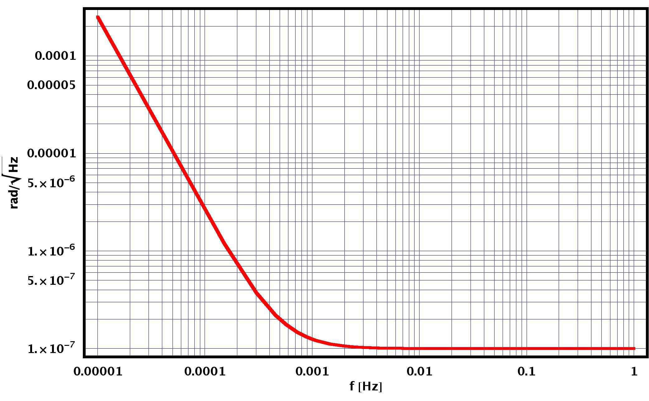
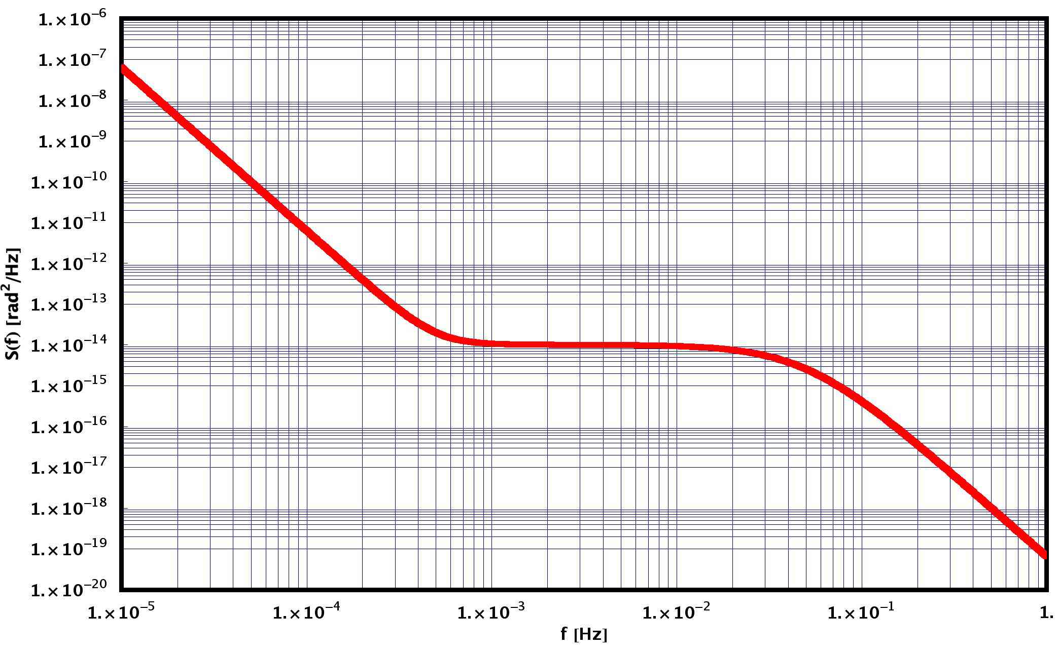
Figure 4.7: Noise from angular displacement sensor (top) and its squared PSD (bottom).

$S_{\dot{\Omega}_{1,\theta}}$, $S_{\dot{\Omega}_{2,\theta}}$

may be deduced from the actuation and measurement noises around $\hat{\theta}$. The two contributions will be square summed, to get:

$$S_{\dot{\Omega}_{1,\theta}}=S_{\dot{\Omega}_{2,\theta}}=\frac{25^{2}+10^{2}}{20.35^{2}}\left|\frac{1.3\times 10^{-11}(s+0.0006)(s+0.0005)^{2}(s+0.0003)}{\left(s+9\times 10^{-5}\right)\left(s+9.5\times 10^{-5}\right)^{2}\left(s+0.0001\right)}\right|^{2}\,\nicefrac{\mathrm{rad^{2}}}{\mathrm{s^{4}\,Hz}}\,.$$ (4.84)

Figure 4.8 depicts both the PSDs $S_{\dot{\Omega}_{1,\theta}}$, $S_{\dot{\Omega}_{2,\theta}}$ and the actuation noise leading to those.

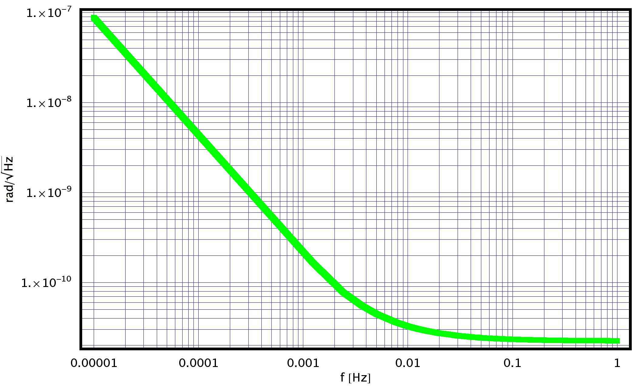
Figure 4.8: Noise from angular actuation (top) and its squared PSD (bottom).

$S_{\dot{\Omega}_{\text{SC},\theta}}$

may be calculated by multiplying each thruster noise times the number of thrusters $(6)$ and considering an effective torsion arm of $1\,\mathrm{m}$:

$$S_{\dot{\Omega}_{\text{SC},\theta}}=\frac{6\times 1\,\mathrm{m}}{(197.4\,\mathrm{kg\,m^{2}})^{2}}\left(10^{-14}+4\times 10^{-8}\frac{1}{\left(1+\frac{\omega^{2}}{\omega_{e,3}^{2}}\right)\left(1+\frac{\omega^{2}}{\omega_{e,4}^{2}}\right)}\right)\,\nicefrac{\mathrm{rad^{2}}}{\mathrm{s^{4}\,Hz}}\,.$$ (4.85)

The value $197.4\,\mathrm{kg\,m^{2}}$ is the measured SC moment of inertia and $\omega_{e,3}=2\pi 0.20\,\mathrm{mHz}$, $\omega_{e,4}=2\pi 0.21\,\mathrm{mHz}$.

$\omega^{2}_{\theta_{1},\theta_{1}}$, $\omega^{2}_{\theta_{2},\theta_{2}}$

may be taken respectively to score $-1.35\times 10^{-6}\,\nicefrac{\mathrm{1}}{\mathrm{s^{2}}}$ and $-2\times 10^{-6}\,\nicefrac{\mathrm{1}}{\mathrm{s^{2}}}$. The reader may find the frequency behaviour of $S_{\dot{\Omega}_{\text{SC},\theta}}$ and the thruster noise figure per single FEEP in picture 4.9.

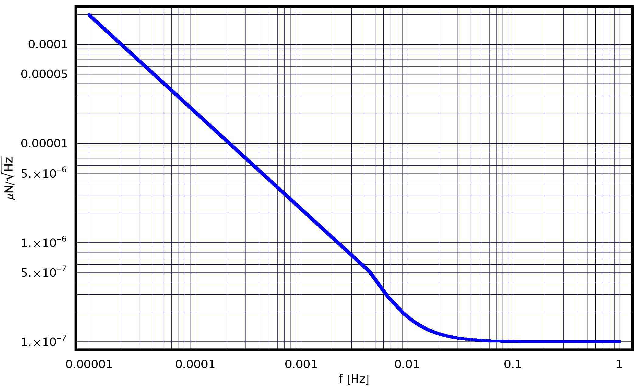
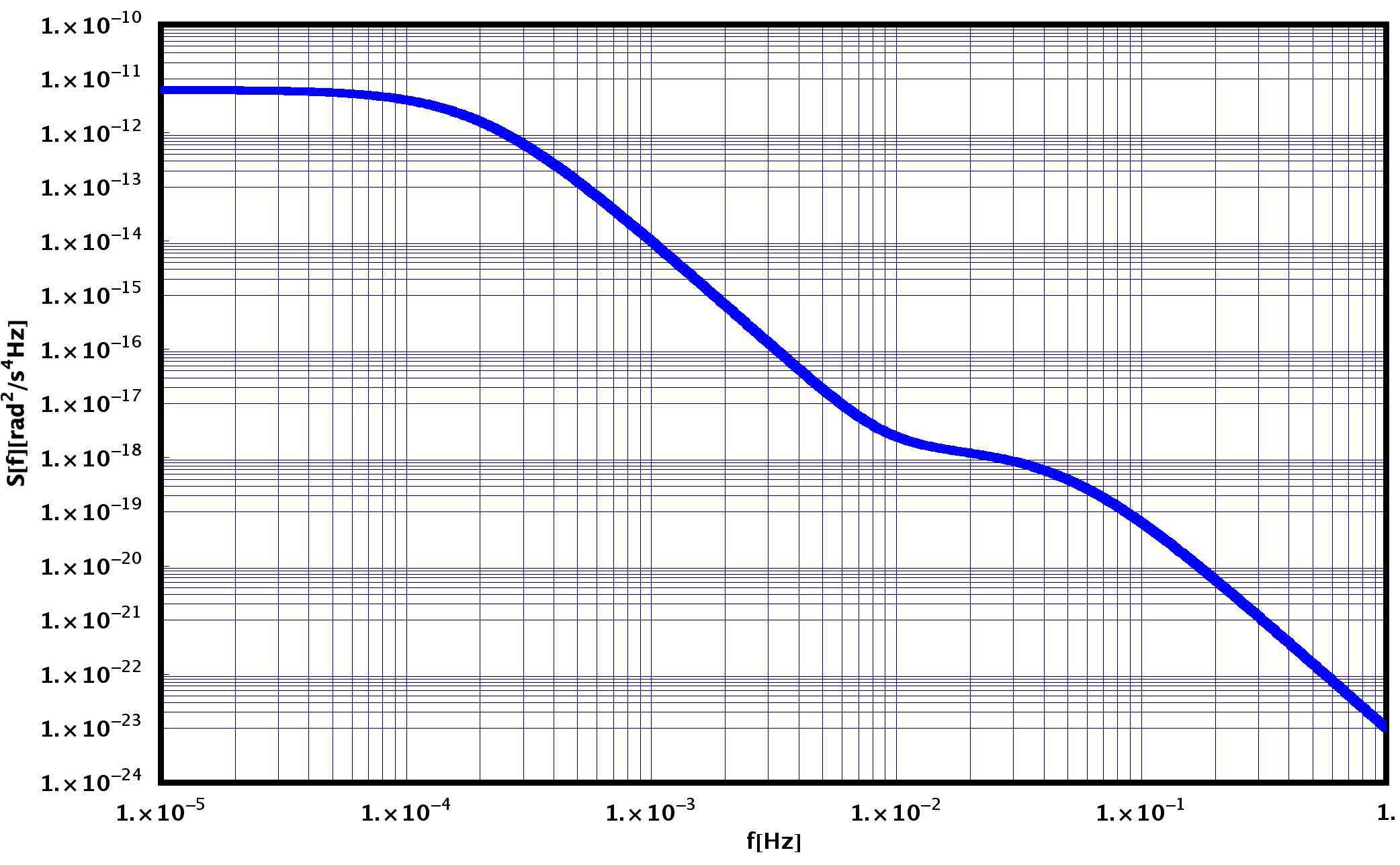
Figure 4.9: Noise from per single thruster (top) and its squared PSD (bottom).

A summary of all the noises together with the total can be found in figure 4.10.

Figure 4.10: Noise summary (top) and its squared PSD (bottom).

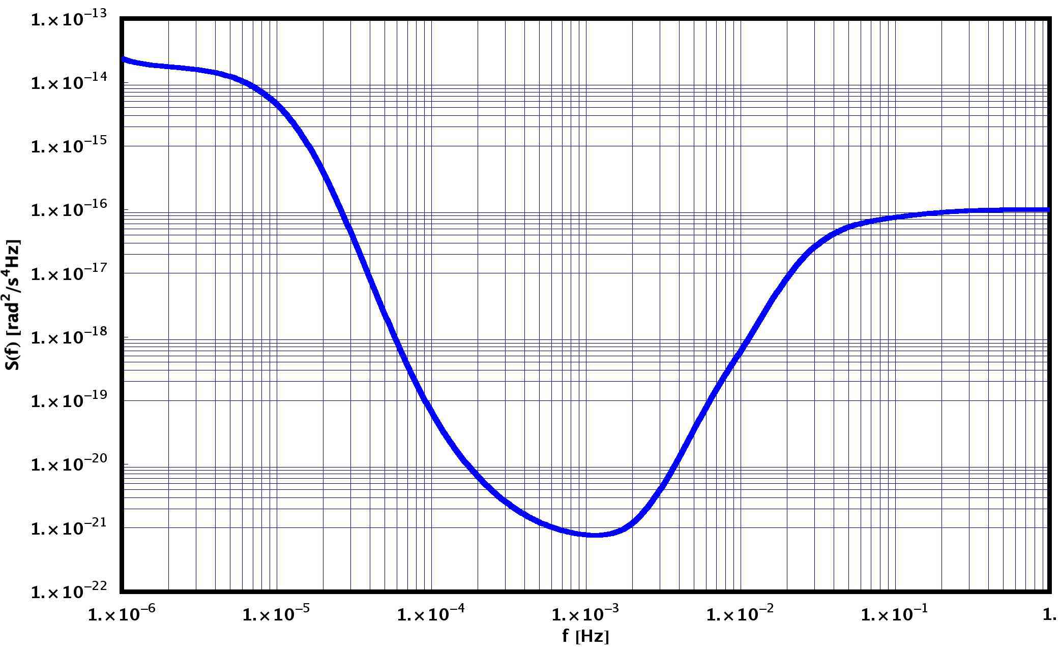
Figure 4.11: PSD of torque noise per unit moment of inertia equivalent to the PSD in (4.82).

4.5.4 Algorithms

In order to estimate the value of accumulated charge an optimal filtering procedure might probably suitable. Nevertheless, the optimal filter requires a detailed knowledge of the noise model and - being this latter a function of time - may cast too demanding a task on the on-board facilities. Many alternative filters have thus been used to proceed in the estimate:

1. continuous time Wiener-Kolmogorov, to evaluate the maximal sensitivity in charge;

2. linear regression to square fitting on a sine signal at discrete time rate, probably being the fastest solution;

3. the former at continuous time, to estimate the data-loss on digitisation;

4. linear regression to square fitting on a sine signal at discrete time rate with a superimposed linear fit;

5. the former at continuous time, same purpose to estimate digitisation loss.

4.5.4.1 Wiener-Kolmogorov filtering

The filter is the same as in section 4.3.1, though we’ll require here a somewhat simpler form for the data:

$$\theta(t)=As(t)+n(t)\,,$$ (4.86)

$A$ being the amplitude we’d like to estimate for the signal $s(t)$, $n(t)$ the relative noise, assumed to be null-average Gaussian distributed. The best estimate of $A$ is:

$$\hat{A}=\frac{1}{\sigma^{2}_{\hat{A}}}\int_{0}^{T}\theta(t)s(t)\operatorname{d}t\,,$$ (4.87)

with

$$\sigma_{\hat{A}}^{2}=\frac{S_{0}}{\int_{0}^{T}s^{2}(t)\operatorname{d}t}\,.$$ (4.88)

Here $S_{0}$ is the noise spectral density, assumed as constant due to the white noise shape (notice it’s always possible to filter the noise so to obtain a white PSD).

4.5.4.2 Linear regression

We can also approximate the data-set in the form of a sine-cosine signal:

$$\theta(t)=c_{s}\sin\omega_{0}t+c_{c}\cos\omega_{0}t\,,$$ (4.89)

where $\omega_{0}$ is the input signal pulsation. The charge can be deduced in terms of $N_{e}$:

$$N_{e}=\frac{\sqrt{c_{s}^{2}+c_{c}^{2}}}{\frac{q_{0}V_{0}}{I_{\theta}}\left|h^{\text{lfs}}_{\theta,\theta_{2},\theta_{2}}\right|}\,.$$ (4.90)

By linear regression fitting, ignoring the noise correlation we can compute the value of the $c_{s}$ and $c_{c}$ coefficients as:

$$c_{i}=\sum_{k=1}^{n}w_{i}(k)\theta(k)\,,\,i=c,s\,,$$ (4.91)

where $n$ is the sample size. The functions $w_{i}(k)$ look like:

$$\begin{split}w_{s}(k)=P(n)\Bigl{(}&\cos\left((2n-(k+1))\omega_{0}\Delta T\right)-\cos\left((k+1)\omega_{0}\Delta T\right)\\ &+2n\sin\left(\omega_{0}\Delta T\right)\sin\left(k\omega_{0}\Delta T\right)\Bigr{)}\,,\end{split}$$ (4.92)

and:

$$\begin{split}w_{c}(k)=P(n)\Bigl{(}&(n-1)\sin\left((k+1)\omega_{0}\Delta T\right)-\sin\left((2n-(k+1))\omega_{0}\Delta T\right)\\ &-n\sin\left((k-1)\omega_{0}\Delta T\right)\Bigr{)}\,,\end{split}$$ (4.93)

with

$$P(n)=-\frac{2n\sin\left(\omega_{0}\Delta T\right)}{1-n^{2}+n^{2}\cos\left(2\omega_{0}\Delta T\right)-\cos\left(2n\omega_{0}\Delta T\right)}\,.$$ (4.94)

Obviously what we carried on til here is a discrete-time analysis, by switching summations to integrals in the former expressions the continuous-time picture can be obtained. This last is used solely for sensitivity purposes.

The linear regression may be complicated with a linear fit superimposed to the sine signal. In this case the data may be approximated by a function in the form:

$$\theta(t)=c_{s}\sin\omega_{0}t+c_{c}\cos\omega_{0}t+a\frac{t}{T}+b\,,$$ (4.95)

with obvious meaning of the symbols. In perfect analogy to what stated already in absence of the straight line term, the formula to determine $N_{e}$ is unvaried from (4.90), as well as the procedure to estimate the $c_{i}$ coefficients. We refer to [11] for details.

4.5.5 Results

Results with different filter strategies have been compared. We report the graph corresponding to the final values of standard deviation per frequency and per strategy. We clearly see the frequency corresponding to the minimum is around $1\,\mathrm{mHz}$, see figure 4.12.

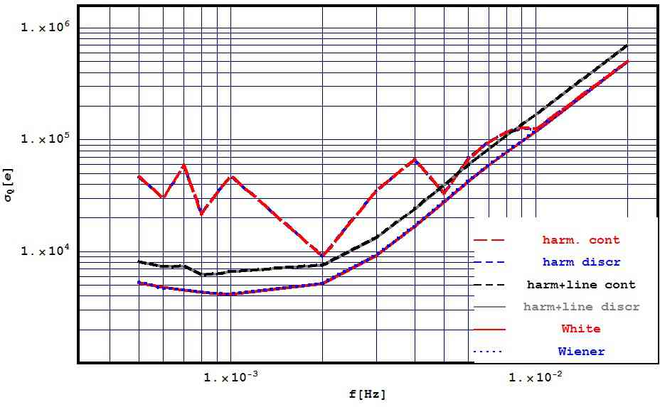
Figure 4.12: Standard deviation per method as function of frequency.

We can also deduce that:

1. a sampling at $1-5\,\mathrm{Hz}$ frequency is enough for a driving force at $1\,\mathrm{mHz}$,

2. the pure sine approximation is inaccurate and the result are strongly dependent on measure duration and data truncation, this failure is highly reduced by the introduction of the linear fitting line to de-trend the data.

In spite of the complications, with a driving frequency of $1\,\mathrm{mHz}$ the sub-optimal filter resolution is of order $6600$ electron charges for $1$ hour time integration and $1\,\mathrm{V}$ amplitude. By accepting a resolution of $10^{5}$ charges the amplitude could be reduced to $50-70\,\mathrm{mV}$, over a measuring time of roughly $2$ hours.

Chapter 5 Fundamental physics with LTP

It was shown in the former chapters that a wave-like gravity perturbation can be accounted for as a local cumulative effect in a global set of coordinates in the form of tidal stretching and shrinking of distances. Moreover, it was shown that it’s possible to build a correspondence between a TT-gauged frame of coordinates and a set of local Fermi-Walker tetrads attached to a laser beam metricised by its pulsation frequency. LTP is then seen as an experimental demonstrator of our ability to build a fiduciary point in free-fall with respect to a very low noise reference. The experiment is born as a technology demonstrator to achieve free-fall up to the level of $3\times 10^{-14}\,\nicefrac{\mathrm{m}}{\mathrm{s^{2}\sqrt{Hz}}}$, but while this remains the primary task of the mission, we can explore a more daring perspective.

By means of reverting the scenario - once we’ve shown that the sensitivity of LTP is the mentioned one and that the operational band is not shaded or reduced in width by unknown or unforecasted phenomena - LTP is - as a matter of fact - a high-precision gradiometer, a spacecraft whose free orbit explores the shape of the gravitational potential, and a gravitational sensor with ability of self-orientation in space. In a word, the perfect projector from TT-gauge to a freely falling tetrad set.

We present in the following some ideas and gedanken tests for a measure of $G$, short and long range violations of the inverse square law, MOND corrections to Newton’s dynamics. Throughout all the chapter we’ll assume a device similar to LTP will be in place, skewed in direction, with the purpose of calibration or gravity signal-generation.

5.1 Introduction

Let’s clear some smoke from the view and sketch some wide-range perspectives as well as list more carefully the tests LTP may be capable of.

1. Though cancelled from the present state of mission, the idea of an internal bona-fide gravity perturbation generator aside LTP could still be pursued. The Disturbance Reduction System DRS (lately renamed as ST7) [60, 61] was meant to be a parallel experiment, to confirm data from LTP aboard the very same SC, and to provide a non-parallel, skewed direction of detection, to test controls mimicking a scenario closer to the one of LISA, where the directions of detection of the TMs would be neither collinear nor orthogonal. In brief, the presence of an oscillatory perturbation generator could provide a carefully tuned signal from a source independent of LTP, useful for calibration purposes but for fine-level measurements too. A measure of $G$ could be planned with such a tool; alternatively, one of the two LTP TM can be moved as to induce a gravitational signal on the other TM. In principle the result would be the same, practically having an independent source would rule out some of the instrumental noise contamination.

2. Dynamics of moving bodies is carefully described to low velocities and mesoscopic scales by means of Newton law, stating that the mutual acceleration between two bodies is a linear function of the square inverse of the mutual distance. Deviations from this law may pick up several forms, but we’ll discuss here three different ones, with links to recent developments from the theory and in adherence to what we think LTP could measure for real.

   Short range violations

   of the inverse square law (ISL) may come out of effective field-theory models which describe possible corrections having exponential form. Hence the additional composition-independent Yukawa potential (i.e. just coupling to mass), can be parametrised as

   $$V_{\text{N}+\text{Y}}(r)=G\frac{m_{1}m_{2}}{r}\left(1+\alpha\exp\left(-\frac{r}{\lambda}\right)\right)\,,$$ (5.1)

   where $\alpha$ characterises the strength of the interaction (relative to gravitation) and $\lambda$ its range. The resulting force is then given by

   $$\begin{split}F_{\text{N}+\text{Y}}(r)&=G\frac{m_{1}m_{2}}{r^{2}}\left(1+\alpha\left(1+\frac{r}{\lambda}\right)\exp\left(-\frac{r}{\lambda}\right)\right)=\\ &=G\frac{m_{1}m_{2}}{r^{2}}\left(1+\xi_{\text{Y}}(r)\right)\,.\end{split}$$ (5.2)

   Short range tests can be carried on by means of using the proof-mass/calibration-mass scheme.

   Long range violations

   of the ISL may occur as well as s.r. ones, and can be a result of a similar potential correction.

   MOdified Newtonian Dynamics

   in the recent and more convincing field-theoretical reformulation of a bi-metric theory of gravity (TeVeS) is a serious competitor to Dark Matter in contemporary cosmology. Its low-velocities approximation builds up an alternative scale-dependent theory of dynamics where the physical gravitational potential $\Phi$ is determined by the modified Poisson equation:

   $${\boldsymbol{\nabla}}\cdot\left(\tilde{\mu}\left(\frac{\left|{\boldsymbol{\nabla}}\Phi\right|}{a_{0}}\right){\boldsymbol{\nabla}}\Phi\right)=4\pi G\tilde{\rho}\,,$$ (5.3)

   where $\tilde{\rho}$ is the baryon’s (only!) mass density, $a_{0}\simeq 10^{-10}\,\nicefrac{\mathrm{m}}{\mathrm{s^{2}}}$ is Milgrom’s characteristic acceleration, and $\tilde{\mu}(x)$ is a free function constrained on the extrema as:

   $$\tilde{\mu}(x)\underset{x\ll 1}{\to}x\,,\qquad\tilde{\mu}(x)\underset{x\gg 1}{\to}1\,.$$ (5.4)

   The physical acceleration is retrieved as ${\boldsymbol{a}}=-{\boldsymbol{\nabla}}\Phi$, and matches the Newtonian prediction for $a\gg a_{0}$. The naîve version of the theory, known as MOND, has been phenomenologically successful in fitting data from galactic rotational curves and at explaining other anomalies, such as the Pioneer one, without invoking additional matter distribution in space other than the baryon’s one. Following Bekenstein and Magueijo [62] we’ll discuss a possible strategy of direct measurement for LTP crossing in a weak MOND region.

   Similarly, the orbit of LTP could be used as a dynamical estimator of the underlying gravity potential. When (if?) crossing close to a Newtonian force saddle point (SP) (${\boldsymbol{F}}(x_{\text{SP}})={\boldsymbol{0}}$), acceleration could be close enough to the scale $a_{0}$ to reveal MOND phenomena.

   LTP is going to be placed in a free Lissajous orbit [38] around L1 (see picture 1.14), the Lagrangian point between Earth and the Sun. The space-probe will get there following a pretty much complicated orbit, which we are not going to describe in detail: picture 1.13, right and 1.14 can be of some help focusing the scenario. While moving, LTP will experience forces and gradients characteristic of the solar system both on the Sun-Earth line, on the ecliptic plane as well as transverse forces and gradients on the Lissajous orbit. A review of these pulls is given in table 5.1; notice the total of forces is obviously $0$ being on orbit.

Heliocentric Orbit - L1	Sun		Earth		Inertial		Total
Force $(\mathrm{N})$	$-1$.	$18\times 10^{-2}$	$3$.	$\times 10^{-4}$	$1$.	$15\times 10^{-2}$	$0$.
Radial gradients $(\nicefrac{\mathrm{N}}{\mathrm{m}})$	$1$.	$59\times 10^{-13}$	$1$.	$65\times 10^{-13}$	$-7$.	$74\times 10^{-14}$	$2$.	$47\times 10^{-13}$
Lissajous Orbit
Force $(\mathrm{N})$	$-5$.	$98\times 10^{-5}$	$-1$.	$.24\times 10^{-4}$	$1$.	$83\times 10^{-4}$	$0$.
Radial gradients $(\nicefrac{\mathrm{N}}{\mathrm{m}})$	$-7$.	$93\times 10^{-14}$	$-1$.	$65\times 10^{-13}$	$-2$.	$45\times 10^{-13}$	$-4$.	$89\times 10^{-13}$

Table 5.1: Detail of modulus of forces and their gradients in Heliocentric, L1 premises and Lissajous orbits. Contributions are split into those given by Sun and Earth and the inertial ones, self-induced by LTP. Totals aside. Obviously, radial gradients for Heliocentric orbit are computed on the Sun-Earth line, while computation for the Lissajous orbit is transverse to the former.

5.2 Measure of $G$

The measure of $G$ is based on our classical knowledge of gravitation. Newton’s law of gravitation for extensive sources can be stated as follows:

$${\boldsymbol{F}}=G\frac{m_{1}m_{2}}{r^{2}}\Pi\left(L,r\right)\frac{{\boldsymbol{r}}}{r}\,,$$ (5.5)

where $m_{1}$ and $m_{2}$ are masses, ${\boldsymbol{r}}$ being the mutual distance vector in three-dimensional space, and $\Pi$ is a form function accounting for the finiteness of the proof-masses, whose characteristic side-scale is summarised by the length $L$. Obviously, in general:

$$\Pi(L,r)\underset{r/L\to\infty}{\to}1\,,$$ (5.6)

because of consistency arguments with the point-like version of Newton’s law.

$G$, Newton’s gravitational constant has current accepted value coming from ground-based experiments of:

$$G=6.6742\times 10^{-11}\,\nicefrac{\mathrm{m^{3}}}{\mathrm{kg\,s^{2}}}\,,$$ (5.7)

with relative uncertainty of $1.5\times 10^{-4}$, i.e. absolute measuring error of $10^{-4}\,\nicefrac{\mathrm{m^{3}}}{\mathrm{kg\,s^{2}}}$. Such a resolution is quite poor in comparison of other fundamental constants, such as for example Planck’s $h$, known with relative uncertainty of $1.7\times 10^{-7}$. Hence, a new measurement by LTP would at least provide the novelty of being carried on in space, off-ground and could possibly improve precision or being competitive with the existing estimate.

A simple measurement of $G$ can be carried on as follows. Let’s consider the two TMs of LTP (but it may be also one of LTP TMs and an external mass oscillating to produce an educated disturbance signal), the gravitational force between them can be expressed by eq. (5.5), by means of moving TM2 by an amount ${\delta}r$ the shift in gravitational force in modulus is

$${\delta}F=-2G\frac{m_{1}m_{2}}{r^{3}}\Pi(L,r){\delta}r\,,$$ (5.8)

i.e. as it is well known:

$$\frac{{\delta}F}{F}=-2\frac{{\delta}r}{r}\,.$$ (5.9)

Such an imbalance in force induces a motion in TM1 which we can model in frequency space by means of our usual main spring-coupling model, introducing an effective spring constant $k_{1}$:

$${\delta}F=\left(m_{1}\omega^{2}-k_{1}^{2}\right){\delta}x\,,$$ (5.10)

where now we named the main detection axis motion after ${\delta}x$. Grouping and solving, we get that the measurement of $G$ will come from:

$$G=\frac{r^{3}\left(k_{1}-\omega^{2}m_{1}\right){\delta}x}{2\Pi(L,r)m_{1}m_{2}{\delta}r}\,.$$ (5.11)

Notice to this level that systematically $G=G({\delta}x,{\delta}r,\omega)$, meaning the values we’ll get from the former formula will be strongly dependent on the strategy of inducing motion in TM1 due to TM2, the detection frequency and more than everything the sensitivity of the detection apparatus. Identifying ${\delta}x\simeq\text{IFO}(x_{2}-x_{1})$ it is obvious that the residual jitter of TM1 can be a serious source of noise spoiling the precision of the measurement. In first place then the true value of $G$ will be a wise averaging $\left\langle G\right\rangle$ on a set of frequencies and shaking schemes of the source.

It is transparent that in order to be competitive with the existing estimates the precision on the constants at play must be maximised. By means of straightforward error propagation analysis, we get the relative variation of $G$ to be:

$$\begin{split}\left(\frac{{\delta}G}{G}\right)^{2}=&\frac{9\epsilon_{r}^{2}}{r^{2}}+\frac{\epsilon_{{\delta}r}^{2}}{{\delta}r^{2}}+\frac{\epsilon_{{\delta}x}^{2}}{{\delta}x^{2}}+\frac{\epsilon_{\Pi}^{2}}{\Pi^{2}}+\frac{4\omega^{2}m_{1}^{2}\epsilon_{\omega}^{2}}{\left(k_{1}-\omega^{2}m_{1}\right)^{2}}+\\ &+\frac{\epsilon_{k_{1}}^{2}}{\left(k_{1}-\omega^{2}m_{1}\right)^{2}}+\frac{k_{1}^{2}\epsilon_{m_{1}}^{2}}{m_{1}^{2}\left(\omega^{2}m_{1}-k_{1}\right)^{2}}+\frac{\epsilon_{m_{2}}^{2}}{m_{2}^{2}}\,,\end{split}$$ (5.12)

where we indicated the uncertainties relative to each variable at play with the symbol $\epsilon$ and the variable name as subscript. The given quantities in this game are shown in table 5.2, together with the uncertainty. We can summarise the main cause inducing relative error as follows:

masses

cannot be easily estimated beyond a certain level due to imprecision in measuring distances while machining. Weight - the first issue in estimating gravitational forces - is thus affected; pre-flight metrology and an accurate mass weighting is the only way to reduce these contributions;

mutual distances

between LTP components get lower bounds on precision because of engineering tolerances; absolute TMs placements to $200\,\mathrm{nm}$ and a strict pre-flight policy to measure displacements within $100\,\mathrm{nm}$ in both sensors is foreseen as a cleanliness method;

distances

are dynamically measured by the GRS and IFO signals. Design sensitivity limits are placed in form of spectral sensitivity curves and cast errors on length estimates, both of the source and of the “sensor”; nothing on this side can be done more than working in the most sensitive bands of the spectrum, such as around frequencies of order $10^{-2}$ till $10^{-3}\,\mathrm{Hz}$. Time integration ranges correspondingly from $3\times 10^{11}$ to $3\times 10^{7}\,\mathrm{s}$ in order to achieve the demanded precision of $10^{-5}$;

stiffness

is dynamically measured with an error induced by the control loop precision and gets more demanding at lower frequency.

Parameter	Nominal value		Relative error		Requirement
$m_{1}$	$1$.	$95$ kg	$6$.	$\times 10^{-4}$	$8$.	$\times 10^{-3}$
$m_{2}$	$1$.	$95$ kg	$6$.	$\times 10^{-4}$	$2$.	$\times 10^{-6}$
$r$	$0$.	$30$ m	$3$.	$\times 10^{-4}$	$6$.	$\times 10^{-7}$
${\delta}r$	$2$.	$\nicefrac{\mathrm{nm}}{\mathrm{\sqrt{Hz}}}$	$2$.	$\times 10^{-6}\,\nicefrac{\mathrm{1}}{\mathrm{\sqrt{Hz}}}$	$3$.	$\times 10^{-6}$
${\delta}x$	$2$.	$\nicefrac{\mathrm{nm}}{\mathrm{\sqrt{Hz}}}$	$1$.	$7\times 10^{-6}\,\nicefrac{\mathrm{1}}{\mathrm{\sqrt{Hz}}}$	$3$.	$\times 10^{-6}$
$k_{1}$	$1$.	$\times 10^{-6}$	$0$.	$1$	$2$.	$\times 10^{-2}$

Table 5.2: Tolerances and estimated uncertainties in key parameters for measurement of $G$ up to precision $10^{-5}$. The column of number named as requirements can be multiplied by $10$ if deemed precision is reduced to $10^{-4}$; conversely integration time can be reduced by two orders of magnitude.

Parameter	Value
${\delta}r$	$1$.	$0\times 10^{-3}\,\mathrm{m}$
${\delta}x$	$1$.	$2\times 10^{-9}\,\mathrm{m}$
$F$	$2$.	$8\times 10^{-9}\,\mathrm{N}$
${\delta}F$	$9$.	$4\times 10^{-12}\,\mathrm{N}$

Table 5.3: Figures of force and its variation for amplitude of modulation or order $10^{-3}\,\mathrm{m}$. Frequency of evaluation is $10^{-2}\,\mathrm{Hz}^{-\nicefrac{{1}}{{2}}}$

The presence of an independent source of educated noise could be of extreme value in the perspective of measurement of $G$ and in the other tests we’ll mention. The ST-7 (DRS) experiment [61] was planned aside LTP on the very same spacecraft and has been mentioned already. In absence, a controlled “gravity generator” (like a couple of rotating spheres joined by a rod) could be regarded as a good source. In place of it, we can consider DRS to be still operational in what follows.

A picture of the mutual DRS-LTP positioning can be inspected in figure 5.1, where laser lines have been emphasised for dramatisation. A detail of the DOF for each DRS TM are shown in picture 5.2.

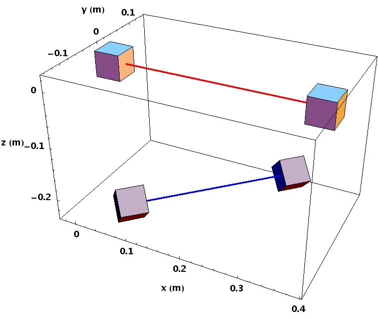
Figure 5.1: LTP and DRS mutual positioning and main laser beams.

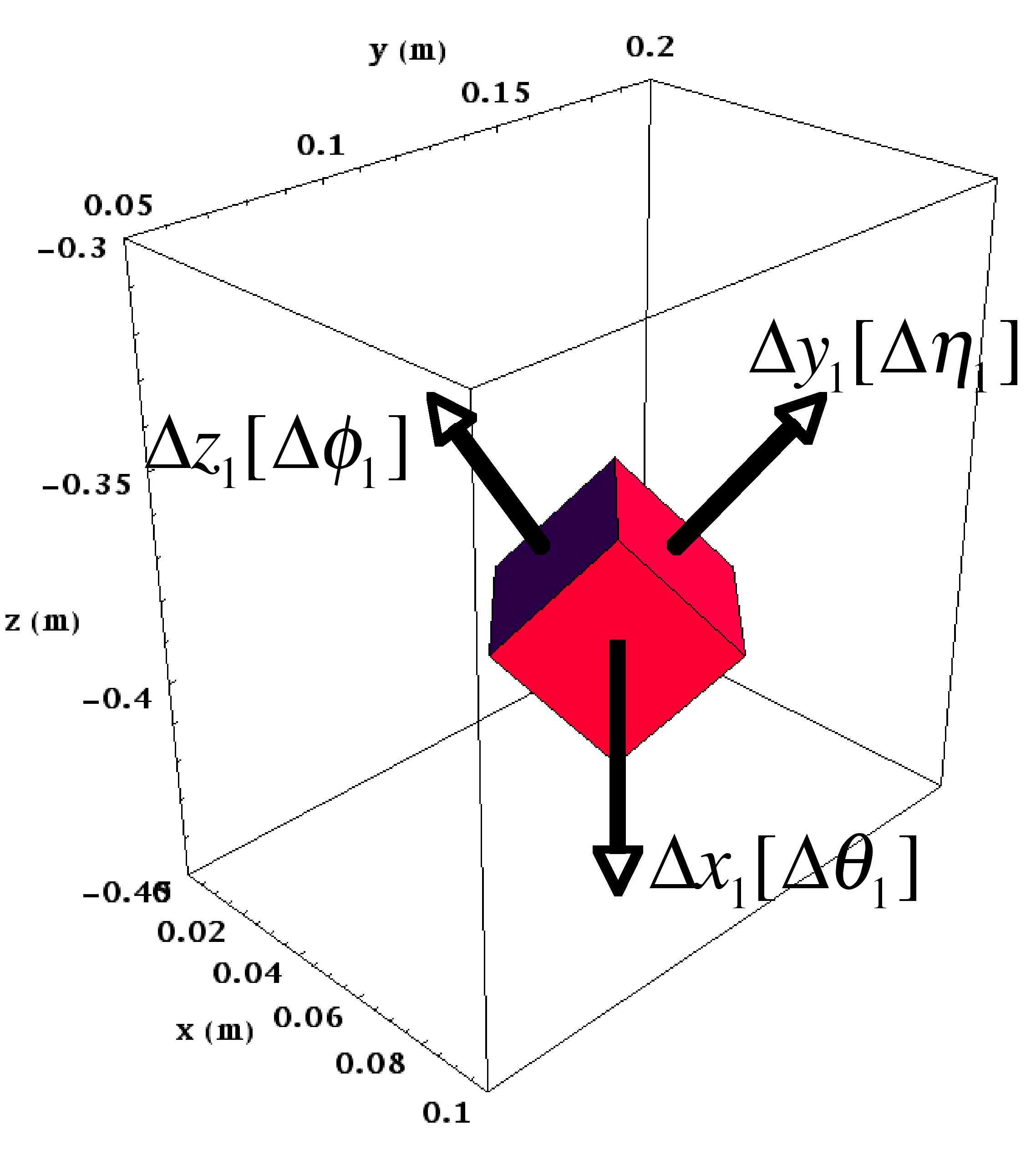
Figure 5.2: DRS TM degrees of freedom.

Measuring $G$ with a DRS+LTP joined operation is not hard to describe. The whole consists into shaking DRS TMs in a proper manner and reading the effect on LTP’s ones. More formally we could say that by a careful control procedure we’d read the phase of the laser locked on the DRS TMs mutual distance after modulating this latter via its GRS system; together, we’d read the effect on the LTP TMs, one servo-ed drag-free, the other suspended. The analysis can be carried on to first harmonic approximation if the DRS TMs motion can be considered like a stable low-frequency sine in the displacement or attitude.

Several simulations were performed and different DOF used for both the devices, even beyond the IFO readout. We hereby focus on results for a $\Delta x_{\text{DRS}}$ to $\Delta x_{\text{LTP}}$ perturbation: for a motion amplitude of the first DRS TM amounting to $200\,\mathrm{\mu m}$ peak, but tables will show numbers for other interesting coupling modes.

As we stated, the motion along the generic DOF $o_{\text{DRS},i}$ is driven to be sine-like:

$$o_{\text{DRS},i}\simeq A\sin t\omega_{D}\,,$$ (5.13)

with $A>0$ (in metres) and $\omega_{D}$ (in Hertz) the drive frequency. By virtue of a version of (5.5) integrated over cubic source masses to point-like observers (see [7] and [59], improved recently in [63]) the effect was tracked down the LTP masses along each DOF of the latter. In all cases, a certain granularity in the motion was assumed to be non-influent by continuity of the fields, therefore a linear increment step of $10\,\mathrm{\mu m}$ was chosen in discretising the sine motion.

The following fitting expansion was chosen in one dimension for the effect on LTP, generic DOF $o_{\text{LTP},k}$:

$$p\left(o_{\text{LTP},k}\right)=\sum_{j=1}^{n}c_{j}\left(o_{\text{DRS},i}\right)^{j}\,.$$ (5.14)

We assumed the so called “first harmonic” result to be reliable, nevertheless checked the result till the fifth (the system is highly causal due to the distances at play, and we can always assume a sine motion on LTP TMs given a sine motion on DRS TMs apart from a negligible phase). By taking (5.14) together with the form (5.13) for the signal and stopping at fifth harmonic ($n=5$), the amplitude of the induced sine motion looks is non-linear in the stimulus and looks like:

$$c_{1}A+\frac{3c_{3}A^{3}}{4}+\frac{5c_{5}A^{5}}{8}\,.$$ (5.15)

Notice, because of the bounded nature of the signal that

$$\left|p(x)\right|\leq\sum_{j}\left|c_{j}\right|A^{j},$$ (5.16)

so that, in case we’d like to estimate the signal/noise ratio by knowing the error $\sigma$ we can tolerate, we can demand

$$\sum_{j}|c_{j}|A^{j}\geq\frac{\sigma}{\sqrt{T}},$$ (5.17)

where $T$ is the integration time we can sustain. To the first harmonic the previous relation gets simplified to

$$|c_{1}|A\sqrt{T}\geq\sigma,$$ (5.18)

which can be used as a “visibility condition” for the signal, provided the drive displacement (rotation) is small and the coefficients $c_{i}A^{i},i>2$ are small compared to $|c_{1}|A$ . In the specific case of our analysis a fitting error of less than $9$ order of magnitudes w/r to the mean was reached with $n=5$ in the polynomial degree.

The $c_{1}$ fit coefficients can be found in table 5.4 for a driving force with $\omega_{D}=2\pi\times 5\times 10^{-2}\,\mathrm{Hz}$. For a displacement (or equivalent rotation) of DRS TMs amounting to $A=200\,\mathrm{\mu m}$ the product $Ac_{1}$ can be found in table 5.5. We estimated the error with respect to $5$-th harmonic analysis in table 5.6. Notice the first order $c_{1}$ coefficient behaves like a gradient of force (torque), therefore shows the correct symmetries with respect to the DRS and LTP TMs positioning.

Inspection of the tables shows a promising value for the $\nicefrac{{\Delta F_{x}}}{{m}}\sim\omega^{2}{\Delta}x_{\text{LTP}}$ upon the given displacement of $\simeq 2.18\times 10^{-13}\,\nicefrac{\mathrm{m}}{\mathrm{s^{2}}}$. By employing (5.18) over an integration time $T=3600\,\mathrm{s}$ and with $\sigma=\sigma_{\text{LTP},\nicefrac{{\Delta F_{x}}}{{m}}}\simeq 3\times 10^{-14}$ we get a signal to noise ratio of $\sim 435$, very satisfactory given the simplicity of the procedure.

This scheme can be complicated by calling in place the control mode transfer functions. The quality of noise projection boosts up in this case and transients can be plotted and analysed. Picture 5.3 shows the case.

	$\nicefrac{{{\Delta}F_{x}}}{{m}}$		$\nicefrac{{{\Delta}\gamma_{\eta}}}{{I_{\eta}}}$		$\nicefrac{{{\Delta}\gamma_{\phi}}}{{I_{\phi}}}$
${{\Delta}x}_{1}$	$1$.	$09\times 10^{-9}$	$2$.	$33\times 10^{-11}$	$1$.	$06\times 10^{-13}$
${{\Delta}x}_{2}$	$1$.	$09\times 10^{-9}$	$2$.	$33\times 10^{-11}$	$-1$.	$06\times 10^{-13}$
${{\Delta}y}_{1}$	$-1$.	$16\times 10^{-9}$	$-1$.	$57\times 10^{-11}$	$-3$.	$34\times 10^{-13}$
${{\Delta}y}_{2}$	$-1$.	$16\times 10^{-9}$	$-1$.	$57\times 10^{-11}$	$3$.	$34\times 10^{-13}$
${{\Delta}z}_{1}$	$4$.	$07\times 10^{-10}$	$-6$.	$03\times 10^{-13}$	$1$.	$69\times 10^{-12}$
${{\Delta}z}_{2}$	$4$.	$07\times 10^{-10}$	$-6$.	$03\times 10^{-13}$	$-1$.	$69\times 10^{-12}$
${\Delta}\theta_{1}$	$-1$.	$59\times 10^{-15}$	$1$.	$32\times 10^{-16}$	$3$.	$50\times 10^{-17}$
${\Delta}\theta_{2}$	$-1$.	$59\times 10^{-15}$	$1$.	$32\times 10^{-16}$	$-3$.	$50\times 10^{-17}$
${\Delta}\eta_{1}$	$-2$.	$29\times 10^{-15}$	$-2$.	$87\times 10^{-16}$	$9$.	$62\times 10^{-18}$
${\Delta}\eta_{2}$	$-2$.	$29\times 10^{-15}$	$-2$.	$87\times 10^{-16}$	$-9$.	$62\times 10^{-18}$
${\Delta}\phi_{1}$	$1$.	$04\times 10^{-15}$	$-1$.	$51\times 10^{-17}$	$3$.	$34\times 10^{-17}$
${\Delta}\phi_{2}$	$1$.	$04\times 10^{-15}$	$-1$.	$51\times 10^{-17}$	$-3$.	$34\times 10^{-17}$

Table 5.4: $c_{1}$ fitting coefficients in the first harmonic signal (5.18).

	$\nicefrac{{{\Delta}F_{x}}}{{m}}$		$\nicefrac{{{\Delta}\gamma_{\eta}}}{{I_{\eta}}}$		$\nicefrac{{{\Delta}\gamma_{\phi}}}{{I_{\phi}}}$
${{\Delta}x}_{1}$	$2$.	$18\times 10^{-13}$	$4$.	$65\times 10^{-15}$	$2$.	$13\times 10^{-17}$
${{\Delta}x}_{2}$	$2$.	$18\times 10^{-13}$	$4$.	$65\times 10^{-15}$	$-2$.	$13\times 10^{-17}$
${{\Delta}y}_{1}$	$-2$.	$32\times 10^{-13}$	$-3$.	$14\times 10^{-15}$	$-6$.	$67\times 10^{-17}$
${{\Delta}y}_{2}$	$-2$.	$32\times 10^{-13}$	$-3$.	$14\times 10^{-15}$	$6$.	$67\times 10^{-17}$
${{\Delta}z}_{1}$	$8$.	$13\times 10^{-14}$	$-1$.	$21\times 10^{-16}$	$3$.	$38\times 10^{-16}$
${{\Delta}z}_{2}$	$8$.	$13\times 10^{-14}$	$-1$.	$21\times 10^{-16}$	$-3$.	$38\times 10^{-16}$
${\Delta}\theta_{1}$	$-3$.	$17\times 10^{-19}$	$2$.	$64\times 10^{-20}$	$6$.	$99\times 10^{-21}$
${\Delta}\theta_{2}$	$-3$.	$17\times 10^{-19}$	$2$.	$64\times 10^{-20}$	$-6$.	$99\times 10^{-21}$
${\Delta}\eta_{1}$	$-4$.	$58\times 10^{-19}$	$-5$.	$75\times 10^{-20}$	$1$.	$92\times 10^{-21}$
${\Delta}\eta_{2}$	$-4$.	$58\times 10^{-19}$	$-5$.	$75\times 10^{-20}$	$-1$.	$92\times 10^{-21}$
${\Delta}\phi_{1}$	$2$.	$08\times 10^{-19}$	$-3$.	$02\times 10^{-21}$	$6$.	$67\times 10^{-21}$
${\Delta}\phi_{2}$	$2$.	$08\times 10^{-19}$	$-3$.	$02\times 10^{-21}$	$-6$.	$67\times 10^{-21}$

Table 5.5: $c_{1}$ fitting coefficients times $A=200\mathrm{\mu m}$ in the first harmonic signal (5.18).

	$\nicefrac{{{\Delta}F_{x}}}{{m}}$		$\nicefrac{{{\Delta}\gamma_{\eta}}}{{I_{\eta}}}$		$\nicefrac{{{\Delta}\gamma_{\phi}}}{{I_{\phi}}}$
${{\Delta}x}_{1}$	$-6$.	$68\times 10^{-18}$	$-2$.	$87\times 10^{-19}$	$-2$.	$14\times 10^{-20}$
${{\Delta}x}_{2}$	$-6$.	$68\times 10^{-18}$	$-2$.	$87\times 10^{-19}$	$2$.	$14\times 10^{-20}$
${{\Delta}y}_{1}$	$1$.	$87\times 10^{-18}$	$2$.	$33\times 10^{-19}$	$7$.	$26\times 10^{-20}$
${{\Delta}y}_{2}$	$1$.	$87\times 10^{-18}$	$2$.	$33\times 10^{-19}$	$-7$.	$26\times 10^{-20}$
${{\Delta}z}_{1}$	$-9$.	$36\times 10^{-18}$	$-4$.	$32\times 10^{-19}$	$-7$.	$93\times 10^{-21}$
${{\Delta}z}_{2}$	$-9$.	$36\times 10^{-18}$	$-4$.	$32\times 10^{-19}$	$7$.	$93\times 10^{-21}$
${\Delta}\theta_{1}$	$3$.	$17\times 10^{-24}$	$-2$.	$7\times 10^{-25}$	$-4$.	$66\times 10^{-26}$
${\Delta}\theta_{2}$	$3$.	$17\times 10^{-24}$	$-2$.	$7\times 10^{-25}$	$4$.	$66\times 10^{-26}$
${\Delta}\eta_{1}$	$4$.	$57\times 10^{-24}$	$6$.	$03\times 10^{-25}$	$1$.	$54\times 10^{-26}$
${\Delta}\eta_{2}$	$4$.	$57\times 10^{-24}$	$6$.	$03\times 10^{-25}$	$-1$.	$54\times 10^{-26}$
${\Delta}\phi_{1}$	$-2$.	$08\times 10^{-24}$	$3$.	$95\times 10^{-26}$	$-8$.	$32\times 10^{-26}$
${\Delta}\phi_{2}$	$-2$.	$08\times 10^{-24}$	$3$.	$95\times 10^{-26}$	$8$.	$32\times 10^{-26}$

Table 5.6: Correction to first harmonic from third and fifth harmonic contributions. Values in table in comparison to table 5.5 show that the percentage error is confined to order $10^{-6}$.

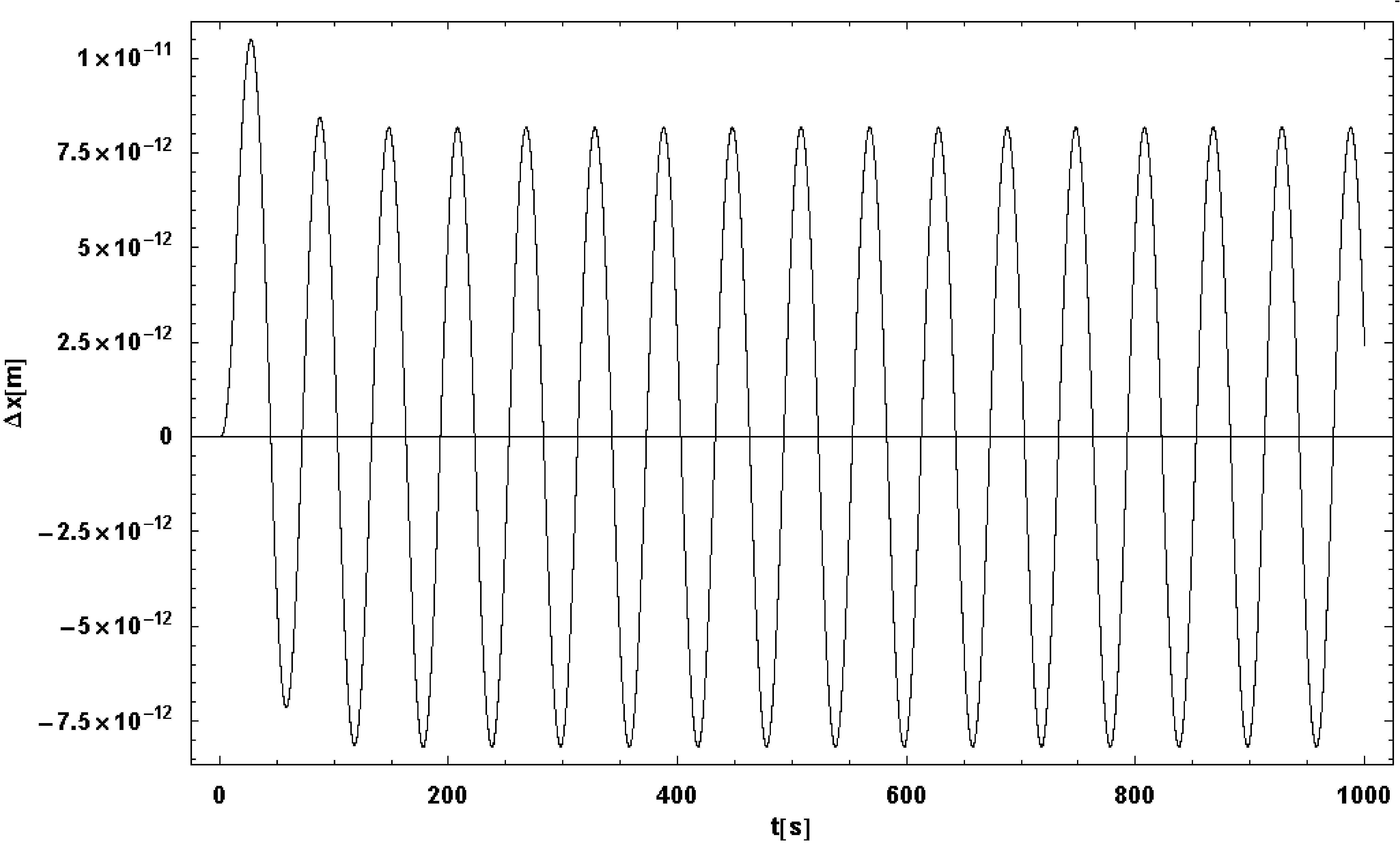
Figure 5.3: Oscillation of LTP TMs mutual distance in response to DRS sine motion. Result from simulation.

5.3 Violation of the ISL

We can consider now the Yukawa-like correction to Newtonian potential expressed by eq. (5.1). In terms of a field-theoretical background such a potential may be motivated as an effective low-energy theory coming from averaged boson interactions (reference here), or as a low-energy by-product from bosonic string theory landscapes. Moreover, given the former potential expression, it’s straightforward to see that

$$V_{N+Y}\underset{\alpha\to 0}{\to}V_{N}\,,$$ (5.19)

and that the correction to acceleration from Newtonian to Yukawa-improved theory scales like

$$\frac{a_{Y+N}}{a_{N}}=1+\alpha\left(1+\frac{r}{\lambda}\right)\exp\left(-\frac{r}{\lambda}\right)\,,$$ (5.20)

which for a large correlation scale $\lambda$ scales to first order like

$$(\alpha+1)+O\left(\left(\frac{1}{\lambda}\right)^{2}\right)\,,$$ (5.21)

thus amounting to an effective renormalisation of the $G$ constant. We can compute then the ratio of difference of acceleration according to the “Y+N” and pure Newton theories at two different working points $r_{1}$ and $r_{2}$ as follows:

$$\begin{split}&\frac{a_{Y+N}\left(r_{1}\right)-a_{Y+N}\left(r_{2}\right)}{a_{N}\left(r_{1}\right)-a_{N}\left(r_{2}\right)}=\\ &=\frac{\frac{1}{r_{1}^{2}}\left(1+\alpha\left(1+\frac{r_{1}}{\lambda}\right)\exp\left(-\frac{r_{1}}{\lambda}\right)\right)-\frac{1}{r_{2}^{2}}\left(1+\alpha\left(1+\frac{r_{2}}{\lambda}\right)\exp\left(-\frac{r_{2}}{\lambda}\right)\right)}{\frac{1}{r_{1}^{2}}-\frac{1}{r_{2}^{2}}}\\ &=1+\frac{\alpha}{r_{2}^{2}-r_{1}^{2}}\left(r_{2}^{2}\left(1+\frac{r_{1}}{\lambda}\right)\exp\left(-\frac{r_{1}}{\lambda}\right)-r_{1}^{2}\left(1+\frac{r_{2}}{\lambda}\right)\exp\left(-\frac{r_{2}}{\lambda}\right)\right)\,,\end{split}$$ (5.22)

it is easy to see that the ratio goes to $1$ as $\alpha\to 0$. It is hence a very good estimator of potential dearths of the theory from Newtonian behaviour at least for a band selection of the $\lambda$ parameter. Notice the ratio is independent on the value of $G$ which we assume independent of the distance.

A short range test can then be performed aboard LTP through two $G$ measurements using two source masses at different distances, namely $G_{1}$ and $G_{2}$. Forgetting about the stiffness correction, we can equate the gravity pull per unit mass to the acceleration in frequency domain (from eq. (5.2)) to get:

$$\frac{G}{r^{2}}\left(1+\alpha\left(1+\frac{r}{\lambda}\right)\exp\left({-\frac{r}{\lambda}}\right)\right)=r\omega^{2}\,,$$ (5.23)

solving and substituting $G\to G_{i}$ for $r\to r_{i}$, we can then rescale each measure so that $G_{i}\to G_{i}r_{i}^{3}$, hence, the $\alpha$ factor can be retrieved as:

$$\alpha=\frac{G_{1}-G_{2}}{G_{1}\left(1+\frac{r_{1}}{\lambda}\right)\exp\left(-\frac{r_{1}}{\lambda}\right)-G_{2}\left(1+\frac{r_{2}}{\lambda}\right)\exp\left(-\frac{r_{2}}{\lambda}\right)}\,.$$ (5.24)

In a similar fashion, a test over long range violations or the ISL can be planned. On purpose the two LTP masses could be used as a gradiometer aligned with the orbit path. Suppose for the time being to consider only one mass $m_{0}$ placed along the Sun-Earth axis, at distance $r_{1}$ from the Sun and $r_{2}$ from Earth. Naming $r_{E}$ the distance Sun-Earth if the Newton $1/r^{2}$ scaling law would apply, we’d get:

$$\begin{split}\Delta a_{S}&=\frac{a_{S}(r_{E})}{r_{1}^{2}}-\frac{a_{S}(r_{1})}{r_{E}^{2}}\,,\\ \Delta a_{E}&=\frac{a_{E}(r_{E})}{r_{2}^{2}}-\frac{a_{E}(r_{2})}{r_{E}^{2}}\,,\end{split}$$ (5.25)

where $a_{E}(r)$ is the Earth’s field acceleration at the radius $r$, $a_{S}(r)$ is the Sun field one. Consequently, since the effect is linear in the accelerations, we get:

$$\Delta a=\Delta a_{S}-\Delta a_{E}\,.$$ (5.26)

If the scaling of the accelerations be Newtonian, we’d expect both (5.25) to be null, thus enforcing (5.26) to be null too. Besides, if each acceleration carries scaling corrections in the form of (5.2), i.e.

$$a_{i}(r)\to a_{\text{N}+\text{Y},\,i}(r)=G\frac{m_{i}}{r^{2}}\left(1+\alpha\left(1+\frac{r}{\lambda}\right)\exp\left(-\frac{r}{\lambda}\right)\right)\,.$$ (5.27)

then a gradiometer effect may arise from (5.26) as the effect of the modified power scaling in the distance:

$$\frac{\Delta a}{a_{S}(r_{E})}=\frac{1}{r_{1}^{2}}\left(1-\frac{1+\xi_{\text{Y}}(r_{1})}{1+\xi_{\text{Y}}(r_{E})}\right)-\frac{1}{r_{2}^{2}}\frac{m_{E}}{m_{S}}\left(1-\frac{1+\xi_{\text{Y}}(r_{2})}{1+\xi_{\text{Y}}(r_{E})}\right)\,,$$ (5.28)

where $a_{S}(r_{E})=5.9\times 10^{-3}\,\nicefrac{\mathrm{m}}{\mathrm{s^{2}}}$ is the Earth acceleration towards the Sun.

Limits in the ISL on large scales can be obtained using SC tracking during transfer mode and during Lissajous orbit. Naturally this implies some requirements:

1. drag-free needs to be operational for the TMs be reliable low-noise detector to build the gradiometer on;

2. SC bias (mainly gravitational forces and gradients) shall be known to high level of accuracy in order to use LTP in alignment with the orbit path and trace gravity gradients;

3. star-trackers in charge of placement of the SC with respect to distant stars carry the most demanding features: in order to achieve an appreciable signal to noise ratio accuracy must be around $30\,\mathrm{\mu m}$. This highly demanding figure seems to place a final shade on the possibility to measure long-range ISL violations.

5.4 MOND

Are MOND [64, 62, 65] effects of importance in the Solar System? Milgrom was the first to consider the effects of MOND on orbits of long period comets from the Oort cloud. Later it was observed that anomalously large perihelia precession of planets fitted predictions from relativistic MOND schemes. The so called “Pioneer anomaly” drew quite some attention and a possible MOND origin of the effect was debated [66, 67, 68].

We’d like to point out some basic facts about MOND:

1. TeVeS [65] encapsulates MOND in a bi-metric scalar-tensor-vector theory of gravity, thus providing a way for the acceleration scale $a_{0}$ to emerge dynamically within the space of parameters as a reference acceleration caused by fields configuration. TeVeS suggests the standard $g_{\alpha\beta}$ metric to be replaced by

   $$\tilde{g}_{\alpha\beta}=e^{-2\phi}g_{\alpha\beta}-2V_{\alpha}V_{\beta}\sinh 2\phi\,,$$ (5.29)

   $\phi$ being a dilaton-type scalar field and $V_{\alpha}$ a four-vector time-like field: $U_{\alpha}U^{\alpha}=-1$. The metric (5.29) collapses to $g_{\alpha\beta}$ for $\phi\to 0$ and the presence of the $V_{\alpha}$ field keeps $\phi$ propagation causal.

2. All the good properties of an action-principle derived theory are respected by TeVeS: locality, invariance and flat-gravity limit of the theory. Causality and positivity of energy are respected.

3. Flat space-time Lagrangians are transposed into TeVeS space-time by switching $g_{\alpha\beta}\to\tilde{g}_{\alpha\beta}$ in indice contractions and by modifying derivatives into co-variant form with respect to $\tilde{g}_{\alpha\beta}$. Integrals are rendered invariant by the Jacobi’s measure $(-\tilde{g})^{\frac{1}{2}}\operatorname{d}^{4}x=e^{-2\phi}(-g)^{\frac{1}{2}}\operatorname{d}^{4}x$, where $\tilde{g}=\det\tilde{g}_{\alpha\beta}$ and $g=\det g_{\alpha\beta}$.

4. Metric ($\tilde{g}_{\alpha\beta}$), Vector ($V_{\alpha}$) and Scalar ($\phi$) equations of motion are obtained by variation of the action $S$. The metric action is the Hilbert-Einstein’s with Ricci tensor written in terms of $\tilde{g}_{\alpha\beta}$. It is of some interest for us only to state that the scalar action carries dependence on the dimensionless parameter $k$ and the length parameter $l$, via a free dimensionless function $\mu$ chosen so to reproduce the MOND phenomenology.

By assuming the matter distribution to be an ideal fluid with density $\tilde{\rho}$ and pressure $\tilde{P}$ we’d get for the $\phi$ field:

$$\left(\mu\left(kl^{2}\phi_{,\nu}\phi^{,\nu}\right)\phi^{,\beta}\right)_{;\beta}=kG(\tilde{\rho}+3\tilde{P})e^{-2\phi}\,,$$ (5.30)

by replacing $g_{\alpha\beta}\to\eta_{\alpha\beta}$ and $e^{-2\phi}\to 1$ and assuming $\tilde{P}$ to be small with respect to $\tilde{\rho}$ we are brought to the set of equations [62]:

$$\begin{split}\nabla\cdot{\boldsymbol{u}}=-4\pi G\tilde{\rho}\,,\\ \nabla\wedge\frac{{\boldsymbol{u}}}{\mu}=0\,,\end{split}$$ (5.31)

where

$${\boldsymbol{u}}=-\frac{4\pi}{k}\mu\nabla\phi\,.$$ (5.32)

Notice $\mu=\mu\left(kl^{2}\left(\nabla\phi\right)^{2}\right)$ is the formerly introduced free-function whose implicit definition could be taken as

$$\frac{\mu}{\sqrt{1-\mu^{4}}}=\frac{k}{4\pi}\frac{\left|\nabla\phi\right|}{a_{0}}\,,$$ (5.33)

and Milgrom’s acceleration $a_{0}$ is recovered as $a_{0}=\nicefrac{{\sqrt{3k}}}{{4\pi l}}\simeq 10^{-10}\,\mathrm{m}{s^{2}}$.

The set of two equations - nonlinear in $\phi$! - (5.31) tell us that ${\boldsymbol{u}}$ equals the Newtonian acceleration ${\boldsymbol{F}}^{(N)}=-\nabla\Phi_{N}$ up to a curl which gets fixed by the second equation up to a gradient. Thus:

$${\boldsymbol{u}}={\boldsymbol{F}}^{(N)}+\nabla\wedge{\boldsymbol{h}}\,,$$ (5.34)

the whole potential thus given by $\Phi=\Phi_{N}+\phi$ and is recovered by inverting (5.34).

By squaring (5.32), using it in (5.33) and carrying out the curl in the second of (5.31) we are lead to:

$$u^{2}=\left(\frac{4\pi}{k}\right)^{2}\mu^{2}\left|\nabla\phi\right|^{2}\,,$$ (5.35)

$$\frac{u^{2}}{a_{0}^{2}}=\left(\frac{4\pi}{k}\right)^{4}\frac{\mu^{4}}{1-\mu^{4}}\,,$$ (5.36)

$$\frac{\partial\ln u^{2}}{\partial\ln\mu}u^{2}\nabla\wedge{\boldsymbol{u}}+{\boldsymbol{u}}\wedge\nabla u^{2}=0\,.$$ (5.37)

In terms of the dimensionless vector field

$${\boldsymbol{U}}\equiv\left(\frac{k}{4\pi}\right)^{2}\frac{{\boldsymbol{u}}}{a_{0}}$$ (5.38)

(5.31) takes the form:

$$\begin{split}\nabla\cdot{\boldsymbol{U}}&=0\,,\\ 4(1+U^{2})U^{2}\nabla\wedge{\boldsymbol{U}}+{\boldsymbol{U}}\wedge\nabla U^{2}&=0\,,\end{split}$$ (5.39)

where we dropped the source term since we are interested the empty region near the SP. Once ${\boldsymbol{U}}$ has been retrieved, $\nabla\phi$ can be recovered by:

$$-\nabla\phi=\frac{4\pi a_{0}}{k}(1+U^{2})^{\frac{1}{4}}\frac{{\boldsymbol{U}}}{U^{\frac{1}{2}}}\,.$$ (5.40)

The Newtonian limit condition is equivalent to $U\gg 1$, in this case:

$$-\nabla\phi\underset{U\gg 1}{\sim}\frac{4\pi a_{0}}{k}{\boldsymbol{U}}=\frac{k}{4\pi}{\boldsymbol{u}}\,.$$ (5.41)

The SP of the Sun-Earth system is a potential candidate for MOND corrections to Newtonian gravity. We spare the reader from the gory details of the deduction, but we’d like now to focus on the premises of the SP itself and thereby analyse the behaviour of the theory. Till now and in the following, we’re just reviewing [62] and compacting the notation.

A quasi-Newtonian region is defined when $U^{2}\simeq 1$. An estimate of the size and shape might be given dropping the curl term in (5.34) and finding the solution to $U^{2}=1$ by virtue of (5.38). The final shape is that of an ellipsoid:

$$r^{2}\left(\cos^{2}\psi+\frac{1}{4}\sin^{2}\psi\right)=r_{0}^{2}\,,$$ (5.42)

where $r_{0}=\nicefrac{{16\pi^{2}a_{0}}}{{k^{2}A}}$ and $A$ is a parameter hiding the mass and distance peculiarities of the SP [62]:

$$A=2\frac{GM}{r_{s}^{2}}\left(1+\sqrt{\frac{M}{m}}\right)\,.$$ (5.43)

In spherical polar coordinates $(r,\,\psi,\,\phi)$ with origin at the SP, we introduce the Ansatz of splitting the ${\boldsymbol{U}}$ field into a Newtonian and a solenoidal component:

$${\boldsymbol{U}}={\boldsymbol{U}}_{0}+{\boldsymbol{U}}_{2}\,,$$ (5.44)

where ${\boldsymbol{U}}_{2}$ is sourced purely by ${\boldsymbol{U}}_{0}$ to first order and it lacks the $\phi$ component being solenoidal. Therefore the following equations hold:

$$\begin{split}\frac{r_{0}}{r}{\boldsymbol{U}}_{0}&=\frac{1}{4}\left(1+3\cos 2\psi\right){\boldsymbol{e}}_{r}-\frac{3}{4}\sin 2\psi{\boldsymbol{e}}_{\psi}\,,\\ \nabla\cdot{\boldsymbol{U}}_{2}&=0\,,\\ \nabla\wedge{\boldsymbol{U}}_{2}&=-\frac{{\boldsymbol{U}}_{0}\wedge\nabla\left|{\boldsymbol{U}}_{0}\right|^{2}}{4\left|{\boldsymbol{U}}_{0}\right|^{4}}\,.\end{split}$$ (5.45)

Boundary conditions are of paramount importance: ${\boldsymbol{U}}_{2}$ vanishes for $r\to\inf$ so that ${\boldsymbol{U}}\to{\boldsymbol{U}}_{0}$ and the Newtonian field is restored. The inward part of the boundary shifts from almost-Newtonian behaviour till more severe MOND regimes. Moreover, the normal component of ${\boldsymbol{U}}$ must vanish on all boundaries. The solution of the former system (5.45) for the field ${\boldsymbol{U}}_{2}$ with these boundary conditions is:

$${\boldsymbol{U}}_{2}=\frac{r_{0}}{r}\left(H_{1}(\psi){\boldsymbol{e}}_{r}+H_{2}(\psi){\boldsymbol{e}}_{\psi}\right)\,,$$ (5.46)

with

$$\begin{split}H_{1}(\psi)&=\frac{2}{5+3\cos 2\psi}-\frac{\pi}{3\sqrt{3}}\,,\\ H_{2}(\psi)&=\frac{\arctan(\sqrt{3}-2\tan{\frac{\psi}{2}})+\arctan(\sqrt{3}+2\tan{\frac{\psi}{2}})-\frac{\pi}{3}\left(\cos\psi+1\right)}{\sqrt{3}\sin\psi}\,.\end{split}$$ (5.47)

The relevant conclusion for our purposes is that a SP far away from the strong MOND bubble is characterised by a Newtonian component proportional to $r$ together with a magnetic-like perturbation falling off like $\nicefrac{{1}}{{r}}$. By combining (5.40) with (5.46) and the expression for ${\boldsymbol{U}}_{0}$ we find that the extra acceleration felt by test particles is expressed by:

$${\boldsymbol{{\delta}F}}=-\nabla\phi\simeq\frac{4\pi a_{0}}{k}\left({\boldsymbol{U}}_{0}+\frac{{\boldsymbol{U}}_{0}}{4U_{0}^{2}}+{\boldsymbol{U}}_{2}+\ldots\right)\,.$$ (5.48)

The contribution proportional to ${\boldsymbol{U}}_{0}$ are Newtonian in nature, but a new magnetic-like contribution shows up, of the same order of magnitude as the second Newtonian one.

System	$r_{0}\,(\mathrm{km})$
Earth-Sun	$383$
Jupiter-Sun	$9.65\times 10^{5}$
Earth-Moon	$140$

Table 5.7: MOND bubbles major semi-axis lengths for three relevant binary isolated systems in the Solar System.

The “magnetic” term we’ve included in the analysis is hence of great importance. In defining the ellipsoid (5.42), solution of $U^{2}=1$ we also define a turn-point between linear corrections to Newton’s theory and full MOND regime and we can estimate the relative corrections as:

$$\frac{{\delta}F}{F^{(N)}}\sim\left(\frac{4\pi}{k}\right)^{3}\left(\frac{a_{0}}{A}\right)^{2}\frac{1}{r^{2}}=\frac{k}{4\pi}\left(\frac{r_{0}}{r}\right)^{2}\,.$$ (5.49)

We see the correction falls off as $\nicefrac{{1}}{{r^{2}}}$ moving away from the SP and by taking the phenomenological value $k\simeq 0.03$ [65] in the nearby of the bubble is amounts to order $0.25\%$.

Given the expression $r_{0}=\nicefrac{{16\pi^{2}a_{0}}}{{k^{2}A}}$ and the choice of $k$ we made, together with formula (5.43) for $A$, the value of $r_{0}$ can be computed for the SPs between the Earth-Sun, Jupiter-Sun and Earth-Moon systems. Results can be retrieved in table 5.7.

Of course at least two caveat we need to cast:

1. this analysis gets more and more naîve for severe nonlinear MOND corrections, where the effect will become much larger than any prediction of (5.49) and the very expression cannot be believed anymore,

2. the real Solar System has a large number of complications at play, starting from elliptical orbits to being a many-body problem. It is hence sensitive to say that the shape and the size of the MOND bubbles may be affected by such perturbations, but not to leading order, while the location of SPs may change abruptly. Notice locating SPs is a Newtonian physics problem, independent of MOND.

LTP may target and detect MOND effects in spite of their smallness. Background tidal stresses of the Sun-Earth system are of order $A\simeq 10^{-11}\,\mathrm{s}^{-2}$, roughly four order of magnitudes above the sensitivity of LTP. (5.49) displays therefore:

$${\delta}F\simeq F^{(N)}\frac{k}{4\pi}\left(\frac{r_{0}}{r}\right)^{2}\simeq 10^{-13}\left(\frac{r_{0}}{r}\right)^{2}\,\nicefrac{\mathrm{1}}{\mathrm{s^{2}}}\,,$$ (5.50)

solving for $r$ assuming LTP sensitivity for ${\delta}F$ gives the radius the space-probe shall hang around to detect some effect, amounting to be $\sim 10r_{0}=3830\,\mathrm{km}$ for the Sun-Earth system.

Unfortunately, on a Lissajous orbit around L1 - sharing L1 dynamical environment - the MOND stresses will be far too small to be detectable: given $r_{L}$ to be L1 distance from the Sun, then its distance from the Earth will be $R-r_{L}\simeq 1.5\times 10^{6}\,\mathrm{km}$. Conversely, the SP of the Sun-Earth system is at $R-r_{s}\simeq 2.6\times 10^{5}\,\mathrm{km}$ from Earth. Hence L1 is far from SP some ${\Delta}r=r_{s}-r_{L}\simeq 1.24\times 10^{6}\,\mathrm{km}$, bringing the correction in (5.49) to:

$$\frac{{\delta}F}{F^{(N)}}\simeq\frac{k}{4\pi}\left(\frac{r_{0}}{r+{\Delta}r}\right)^{2}\simeq\frac{k}{4\pi}\left(\frac{r_{0}}{{\Delta}r}\right)^{2}\simeq 2.4\times 10^{-10}\,.$$ (5.51)

The background tidal stresses due to Newtonian dynamics at L1 are still high in comparison to LTP sensitivity; e.g. for the radial component:

$$\frac{\partial F^{(N)}}{\partial r}\Bigr{|}_{\text{L1}}\simeq 3.17\times 10^{-13}\,\nicefrac{\mathrm{1}}{\mathrm{s^{2}}}\,,$$ (5.52)

which is two order of magnitudes above the figure of $\sim 10^{-15}\,\nicefrac{\mathrm{1}}{\mathrm{s^{2}}}$. Therefore the game will be to detect corrections $8$ order of magnitudes beneath experimental sensitivity, a thing we cannot believe.

5.5 Conclusions, measurable effects and limitations

At the present status of the mission design, the measure of $G$ seems to be the most promising test of fundamental physics onboard LTP.

Critical parameters may be inspected in table 5.2 with reference to formula (5.12). Let motion be induced by the spare mass of LTP or by virtue of a DRS-like source, the knowledge of the distance parameter is the most troublesome issue. Moreover, in lack of an independent source such as DRS, stiffness may dominate the measure anyway.

The baseline distance $r$ will be known with precision $\sim 10^{-4}$, while the deemed precision shall be $\sim 10^{-7}$; furthermore, what will happen after launch and orbit placement to mutual distance of apparata is predictable only up to some extent. This is not going to affect a differential acceleration measurement, but unless a dedicated calibration tool will be introduced - a fact which is very unlikely to happen - the figure of $\sim 10^{-4}$ precision on $r$ is a real one and a heavy one for the measure of $G$.

In the fortunate case of a thorough calibration of the $k_{1}$ constant in (5.11), the value of $\nicefrac{{{\delta}G}}{{G}}$ will be dominated anyway by $\epsilon_{r}$, thus providing a competitive value for $G$ with regard to the accepted value of (5.7). We fear this occurrence to be too optimistic, it will be rather more preferable to take profit of a dedicated source in place of DRS. As stated, this may take the shape of a two-mass slid, or a rotator with cubic masses, but nothing prevents to think about many little devices to be placed with careful symmetry around the LTP centre of mass, and activated independently at will.

On the converse, with no calibration and no external source, $\epsilon_{k_{1}}$ will dominate the relative uncertainty picture, and $\nicefrac{{{\delta}G}}{{G}}$ will be - optimistically - of order $10^{-1}$… the measure will still be the first one in space, but with no surprises or real scientific value.

As for the test of ISL, we discussed them here for the sake of completeness, but we are not really confident that LTP shall provide news about this argument. Twofold the counter-proof: the static-gravitation analysis which was carried on for gravitational compensation is based on the $\nicefrac{{1}}{{r^{2}}}$ ISL scaling, in case new effects would arise, it might be very hard to discriminate them from this SC-induced background, and anyway a more sophisticated analysis will be needed. In addition, unless the $\epsilon_{k_{1}}$ relative error on stiffness dominance or in turn the $\epsilon_{r}$ distance one will be depressed on the measure of $G$, it is very unlikely the deemed sensitivity will be reached onboard LTP in order to perform a competitive test of the ISL. Again a minor task might be to confirm the $\nicefrac{{1}}{{r^{2}}}$ scaling and standard Newtonian behaviour at L1 and across the orbit.

It may be true that indirect MOND effects may be felt by the orbit of SMART-2; an extra acceleration will be present at L1 pointing toward the SP (away from the Sun, in direction of Earth) may be felt by the SC and seen in the orbit [62].

To give our little contribution to this debate, we frankly think that MOND effects will be very hard to detect by LTP unless a careful numerical estimate of the Sun-Earth SP be made given the many-body influence of the other planets. Once located, the space-probe may be sent in the premises and a measure might be taken.

We have nevertheless three arguments we’d like to share at the end of the chapter:

1. theoretically, MOND doesn’t seem very interesting a solution at mesoscopic level. To clarify the thought, MOND doesn’t come out of any natural quantum scenario and doesn’t look like a consistent or cooperative effect of some fundamental field at play. It is not enough in physics to collect a bunch of fields with some given constants and claim this is a new paradigm. Though curious and astonishing in the remarkable phenomenological success, it is very unlikely that even an experimental test at LTP level would produce unequivocal data to be interpreted as “MOND effects”.

2. At experimental level, perhaps a longer baseline interferometric device could (will?) have better chance to see MOND effects. If used as gradiometers, the SCs of LISA could for example laser-map bubbles around the SPs. These do not behave like GW sources, they are an example of a static, non radiative gravitational deformed region, but whenever a laser beam would move and cross their section it would experience the $\nicefrac{{{\delta}F}}{{F^{(N)}}}$ correction, and the amount of it would be larger the closer to the SP the beam would shine. At the moment we have no numbers or figures to substantiate the picture, but the idea seems promising.

3. The introduction of a time-like field $V^{\mu}$ corresponds to the identification of a preferred time-frame (cosmological, since the action is local and no difference is cast on the form of $V^{\mu}$ from point to point). The metric stretching may be therefore anisotropic. Another chance could be then to perform acceleration difference measurement with the sensing axis of LTP randomly oriented in space and see whether any difference arises (i.e. by moving the whole SC). The large Lissajous orbit and the yearly revolution of SMART-2 might provide a natural envelope of space orientation to explore this scenario.

Appendix A Gravitational waves in Einstein General Relativity

We hereby introduce the concept of gravity waves according to the framework of GR. Equations of motion for wave-like propagation of gravity in space-time are derived from Einstein’s equations in the far-source approximation, polarisation is discussed in relation to the choice of a gauge (the TT-gauge), energy density carried by the waves and the lowest-level quadrupole nature of the sources are introduced and discussed.

Next we’ll gauge to the first part in answering the question on how GWs may be detected and their effect measured by interferometers on small and large scales.

Strains figures and examples will be provided, together with a link to sources frequencies.

The chapter is thought in support to chapter 1 and supposed to provide a more human-readable and common introduction, in fact, what we present here may be regarded as standard text-book material.

A.1 Gravitational waves in Einstein’s theory

The existence of GWs can be deduced starting from two assumptions: Lorentz invariance and local causality: fields are functions of space and time an the requirement of all signals (including the gravitational) to be non-superluminal with respect to the limiting speed scale $c$ forces the propagation in vacuo to be wave-like. If not a full certainty, these facts must at least induce some suspect on the existence of GWs.

GWs can be deduced [69] from Einstein’s relativistic field equations under the approximation of weak field, which accounts on having far sources. No assumptions is a-priori made on time dependence of motion and no restriction is cast on particle motion too.

The weakness of the gravitational field is expressed as our ability to decompose the metric $g_{\mu\nu}$ into flat Minkowski plus a small perturbation $h_{\mu\nu}$, such that $|h_{\mu\nu}|\ll 1$ (a condition which must hold throughout all the following!):

$$g_{\mu\nu}=\eta_{\mu\nu}+h_{\mu\nu}\,.$$ (A.1)

From now on, we will adopt Einstein’s conventions as for Greek indice, i.e. designating four-vectors, Latin indice to address three-vectors, and implied summation over repeated indice. Indice are normally raised or lowered at need by means of the full metric $g_{\mu\nu}$ or its inverse unless otherwise specified. In the case of weak field, $\eta_{\mu\nu}$ and/or its inverse will be used. A comma will identify partial derivative whilst a semicolon a $g_{\mu\nu}$-co-variant one. It can be easily read out of (A.1) that the inverse is

$$g^{\mu\nu}=\eta^{\mu\nu}-h^{\mu\nu}\,.\,.$$ (A.2)

Whenever the symbol ${\boldsymbol{x}}^{2}$ will appear, it will have the meaning of $\sum_{i}x_{i}x_{i}=|{\boldsymbol{x}}|^{2}$.

We’d like now to proceed finding the Christoffel connection symbols:

$$\Gamma^{\rho}_{\phantom{\rho}\mu\nu} =\frac{1}{2}g^{\rho\sigma}\left(g_{\nu\sigma,\mu}+g_{\mu\sigma,\nu}-g_{\mu\nu,\sigma}\right)=$$ (A.3)

$$=\frac{1}{2}\eta^{\rho\sigma}\left(h_{\nu\sigma,\mu}+h_{\mu\sigma,\nu}-h_{\mu\nu,\sigma}\right)\,,$$ (A.4)

and the Riemann tensor expression:

$$R_{\mu\nu\rho\sigma} =g_{\mu\lambda}R^{\lambda}_{\phantom{\lambda}\nu\rho\sigma}=g_{\mu\lambda}\left(\Gamma^{\lambda}_{\phantom{\lambda}\nu[\rho,\sigma]}+\Gamma^{\tau}_{\phantom{\tau}\rho[\nu}\Gamma^{\lambda}_{\phantom{\lambda}\sigma]\tau}\right)=$$ (A.5)

$$=\eta_{\mu\lambda}\Gamma^{\lambda}_{\phantom{\lambda}\nu[\sigma,\rho]}=$$ (A.6)

$$=\frac{1}{2}\left(h_{\sigma[\mu,\nu],\rho}+h_{\rho[\nu,\mu],\sigma}\right)\,.$$ (A.7)

The Ricci tensor is obtained by contracting over $\rho$ and $\sigma$, thus giving:

$$R_{\mu\nu}=g^{\rho\sigma}R_{\mu\nu\rho\sigma}=\frac{1}{2}\left(h^{\sigma}_{\phantom{\sigma}(\mu,\nu),\sigma}-h_{,\nu,\mu}-\square h_{\mu\nu}\right)\,,$$ (A.8)

where we defined the trace $h=\eta^{\mu\nu}h_{\mu\nu}$ and the D’Alembert operator in Minkowski space $\square=\eta^{\mu\nu}\partial_{\mu}\partial_{\nu}$. The Ricci scalar is:

$$R=g^{\mu\nu}R_{\mu\nu}=h^{\mu\nu}_{\phantom{\mu\nu},\nu,\mu}-\square h.$$ (A.9)

With these assumptions, the l.h.s. of Einstein’ equations:

$$E_{\mu\nu}=R_{\mu\nu}-\frac{1}{2}Rg_{\mu\nu}=\frac{8\pi GT_{\mu\nu}}{c^{2}}\,,$$ (A.10)

become:

$$E_{\mu\nu} \to R_{\mu\nu}-\frac{1}{2}R\eta_{\mu\nu}=$$ (A.11)

$$=\frac{1}{2}\left(h^{\sigma}_{\phantom{\sigma}(\mu,\nu),\sigma}-h_{,\nu,\mu}-\square h_{\mu\nu}-\eta_{\mu\nu}h^{\rho\sigma}_{\phantom{\rho\sigma},\sigma,\rho}+\eta_{\mu\nu}\square h\right)=$$ (A.12)

$$=\frac{8\pi GT_{\mu\nu}}{c^{2}}\,.$$ (A.13)

In (A.10) $T_{\mu\nu}$ represents the energy-momentum tensor whose expansion will be considered to zeroth order in $h$. $T_{\mu\nu}$ must be small for the weak-field condition to apply; to lowest order the conservation of energy and momentum simplifies to $T_{\mu\nu;\mu}\to T_{\mu\nu,\mu}=0$.

The field equations (A.11) do not have unique solutions due to general covariance: the same physical situation is represented by different choices of coordinates as:

$$x^{\mu}\to x^{\mu}+\xi^{\mu}\,,$$ (A.14)

so that the perturbation $h_{\mu\nu}$ is related to a transformed other, leaving curvature and hence the physical space-time unchanged. Formally:

$$h_{\mu\nu}\to h_{\mu\nu}+\xi_{(\nu,\mu)}\,.$$ (A.15)

Notice, since $\left|h_{\mu\nu}\right|\ll 1$ that $\xi_{\mu}$ and $\xi_{\mu,\nu}$ must be (infinitesimal) of order $h_{\mu\nu}$. The choice of a gauge is important to simplify the form of the final equations. We choose the harmonic gauge condition:

$$0=g^{\mu\nu}\Gamma^{\lambda}_{\phantom{\lambda}\mu\nu}=h^{\lambda}_{\phantom{\lambda}\mu,\lambda}-\frac{1}{2}h_{,\mu}\,,$$ (A.16)

by introducing $\bar{h}_{\mu\nu}=h_{\mu\nu}-\frac{1}{2}\eta_{\mu\nu}h$ the harmonic gauge reduces to the Lorentz divergence condition $\bar{h}^{\mu}_{\phantom{\mu}\lambda,\mu}=0$ and the linearised Einstein’ equations simplify to:

$$\square\bar{h}_{\mu\nu}=-\frac{16\pi G}{c^{2}}T^{\mu\nu}\,.$$ (A.17)

Outside the source, in empty space $T^{\mu\nu}=0$ and we may drop the r.h.s. of (A.17) thus getting:

$$\square\bar{h}_{\mu\nu}=0\,.$$ (A.18)

Such an equation admits a plane-wave solution of the kind $\bar{h}_{\mu\nu}=A_{\mu\nu}\exp(ik_{\alpha}x^{\alpha})$ where $A_{\mu\nu}$ is a constant, symmetric, rank-2 tensor and $k_{\alpha}=(\omega,{\boldsymbol{k}})$ is the wave vector. Gravitational waves travel at the speed of light and this can be proved by plugging the readily-found solution into (A.18) to find:

$$k_{\alpha}k^{\alpha}=0\,,$$ (A.19)

that is, the world line of a GW is light-like. Moreover, using the linearised harmonic gauge condition we get

$$k_{\alpha}A^{\alpha\beta}=0$$ (A.20)

implying trasversality (orthogonality) of the wave front to $k_{\alpha}$. The remaining gauge d.o.f. in $A_{\mu\nu}$ can be fixed by choosing $\bar{h}_{00}=0$ and $\eta^{\mu\nu}\bar{h}_{\mu\nu}=0$, i.e. the tracelessness. In full, this gauge choice is named after TT-gauge, meaning transverse and traceless. As an effect of the lack of trace we have $\bar{h}^{TT}_{\mu\nu}=h^{TT}_{\mu\nu}$. Choosing now to meet the GW along our $\hat{z}$ direction, we have

$$k_{\mu=0..3}\to(\omega,0,0,\omega)\,,$$ (A.21)

which implies $A_{\alpha 3=0}$ and we are left with [70]

$$A_{\mu\nu}^{TT}=\left[\begin{matrix}0&0&0&0\\ 0&A_{11}&A_{12}&0\\ 0&A_{21}&-A_{11}&0\\ 0&0&0&0\end{matrix}\right]=\left[\begin{matrix}0&0&0&0\\ 0&h_{+}&h_{\times}&0\\ 0&h_{\times}&-h_{+}&0\\ 0&0&0&0\end{matrix}\right]\,,$$ (A.22)

and the two a-dimensional lengths $h_{+}$ an $h_{\times}$ completely characterise the wave “amplitude”.

A.2 Sources and energy-momentum

Back to equation (A.17), a general solution can be found by means of Green’s function formalism [69, 71], to give:

$$\bar{h}_{\mu\nu}(t,{\boldsymbol{x}})=\frac{4G}{c^{2}}\int\operatorname{d}^{3}y\frac{T_{\mu\nu}(t-\frac{|{\boldsymbol{x}}-{\boldsymbol{y}}|}{c},{\boldsymbol{y}})}{|{\boldsymbol{x}}-{\boldsymbol{y}}|}\,,$$ (A.23)

where the retarded time $t_{R}=t-\nicefrac{{|{\boldsymbol{x}}-{\boldsymbol{y}}|}}{{c}}$ accounts for the disturbance of the gravitational field at present coordinates $(t,{\boldsymbol{x}})$ to be the superposition of influences from energy and momentum sources at $(t_{R},{\boldsymbol{y}})$ on the past light cone.

Under the assumption of being far from the source, considered point-like in its spatial extent compared to the distance ($|{\boldsymbol{y}}|\ll|{\boldsymbol{x}}|$), we get

$$\bar{h}_{\mu\nu}(t,{\boldsymbol{x}})=\frac{4G}{c^{4}|{\boldsymbol{x}}|}\int T_{\mu\nu}\left(t-\frac{|{\boldsymbol{x}}|}{c},{\boldsymbol{y}}\right)\operatorname{d}^{3}y\,,$$ (A.24)

and by means of the sources identity and definition of quadrupole moment

$$\int T^{jk}\operatorname{d}^{3}x=\frac{1}{2}\frac{\partial^{2}}{\partial t^{2}}\int T^{00}x^{j}x^{k}\operatorname{d}^{3}x\,,$$ (A.25)

$$q_{jk}\doteq\int T^{00}x^{j}x^{k}\operatorname{d}^{3}x\,.$$ (A.26)

Notice anyway that neither side of (A.24) is transverse or traceless with respect to the observation direction. We need therefore to introduce projectors onto the plane with normal ${\boldsymbol{n}}\doteq\nicefrac{{{\boldsymbol{x}}}}{{\left|{\boldsymbol{x}}\right|}}$:

$$P_{jk}\doteq\delta_{jk}-n_{j}n_{k}\,,$$ (A.27)

and combine them in a TT projector:

$$P^{\text{TT}}_{jkmn}\doteq P_{jm}P_{kn}-\frac{1}{2}P_{jk}P_{mn}\,,$$ (A.28)

so that, for the newly defined $q_{jk}$ we’d get:

$$q^{\text{TT}}_{jk}=P^{\text{TT}}_{jkmn}q_{mn}\,,$$ (A.29)

and finally from (A.24):

$$\bar{h}^{\text{TT}}_{jk}(t,{\boldsymbol{x}})=\frac{2G}{c^{4}|{\boldsymbol{x}}|}\frac{\operatorname{d}^{2}q^{\text{TT}}_{jk}}{\operatorname{d}t^{2}}\Big{|}_{t-\nicefrac{{|{\boldsymbol{x}}|}}{{c}}}\,,$$ (A.30)

therefore showing the gravitational field produced by an isolated non-relativistic object is proportional to the second time derivative of the TT-projected quadrupole moment of the energy density at the point where the past light cone of the observer intersects the source. The universal nature of gravitation is therefore quadrupolar to lowest order due to mass and momentum conservation, elucidating also the weakness of the interaction, generally smaller than dipolar EM one.

The canonical energy-momentum pseudo-tensor (Landau) carried by gravitational waves can be obtained from the usual field-theory formalism:

$$t_{\mu\nu}=\frac{1}{32\pi G}\left\langle h^{TT}_{\rho\sigma,\mu}h^{TT\rho\sigma}_{\phantom{TT\rho\sigma},\nu}\right\rangle\,,$$ (A.31)

where the r.h.s. has been averaged over several wavelengths, to circumvent a definition of local gravitational field - a nonsense for GW due to the existence of Riemann normal coordinates [19]. Moreover the averaging has the practical meaning to capture more information on the physical curvature of a small region to describe a gauge-invariant measure.

Finally we can compute the luminosity of a source:

$$L_{\text{GW}}=-\frac{\operatorname{d}W_{\text{GW}}}{\operatorname{d}t}=\frac{G}{5c^{5}}\left\langle\left(\frac{\operatorname{d}^{3}Q_{jk}}{\operatorname{d}t^{3}}\right)^{2}\right\rangle\Big{|}_{t-\frac{|{\boldsymbol{x}}|}{c}}\,,$$ (A.32)

in terms of its traceless (reduced) quadrupole tensor

$$Q_{jk}=\int\left(x^{j}x^{k}-\frac{1}{3}{\boldsymbol{x}}^{2}\delta_{jk}\right)T^{00}\operatorname{d}^{3}x\,.$$ (A.35)

A.3 Effects on test particles

Let’s consider the effect of gravitational waves on test particles and moving bodies [71, 19] in their proper frame of reference. If we take two particles in free-fall, described by a single velocity field $U^{\alpha}=\frac{\operatorname{d}x^{\alpha}}{\operatorname{d}\tau}$, where $\tau$ is the proper time, it is well known that the separation vector $X^{\alpha}$ obeys the equation of geodesic deviation (see (B.39)):

$$\frac{\operatorname{d}^{2}X^{\mu}}{\operatorname{d}\tau^{2}}+\Gamma^{\mu}_{\phantom{\mu}\sigma\rho}\frac{\operatorname{d}X^{\rho}}{\operatorname{d}\tau}\frac{\operatorname{d}X^{\sigma}}{\operatorname{d}\tau}=R^{\mu}_{\phantom{\mu}\nu\rho\sigma}U^{\nu}U^{\rho}X^{\sigma}\,,$$ (A.36)

considering only the lowest-order components of $U^{\nu}$, we can take $U^{\nu}=\delta^{\nu}_{\phantom{\nu}0}$ pointing in the time direction $\hat{t}$ and $X^{\nu}=\delta^{\nu}_{\phantom{\nu}1}$ along $\hat{x}$. To first order in $h_{\mu\nu}$ we get from (A.36):

$$\frac{\operatorname{d}^{2}X^{\mu}}{\operatorname{d}t^{2}}=R^{\mu}_{\phantom{\mu}00\sigma}X^{\sigma}\,.$$ (A.37)

This expression of the Riemann tensor can be calculated in linearised theory:

$$R^{\mu}_{\phantom{\mu}00\sigma} =\eta^{\mu\alpha}\frac{1}{2}\left(h^{TT}_{\alpha\sigma,0,0}+h^{TT}_{00,\alpha,\sigma}-h^{TT}_{\mu 0,0,\sigma}-h^{TT}_{\sigma 0,0,\alpha}\right)=$$ (A.38)

$$=\frac{1}{2}\eta^{\mu\alpha}h^{TT}_{\alpha\sigma,0,0}\,,$$ (A.39)

where we used again $h^{TT}_{\mu 0}=0$. Thus equation (A.37) becomes:

$$X^{\mu}_{\phantom{\mu},0,0}=\frac{1}{2}\eta^{\mu\alpha}h^{TT}_{\alpha\sigma,0,0}X^{\sigma}\,.$$ (A.40)

If the incoming gravitational perturbation is characterised by an amplitude tensor of the form (A.22) and it has got the form of a plane wave - which is locally likely to be, due to the distance from the sources - the test particles will only be disturbed in directions $\hat{x}$ and $\hat{y}$, orthogonal to the wave vector. Suppose for illustration to choose $h_{\times}=0$ so that:

$$\begin{split}X^{1}_{\phantom{1},0,0}&=\frac{1}{2}X^{1}\left(h_{+}\exp(ik_{\lambda}x^{\lambda})\right)_{,0,0}\\ X^{2}_{\phantom{2},0,0}&=-\frac{1}{2}X^{2}\left(h_{+}\exp(ik_{\lambda}x^{\lambda})\right)_{,0,0}\,;\end{split}$$ (A.41)

To first order in the wave phase, we get:

$$\begin{split}\ddot{X}^{1}&=\frac{1}{2}X^{1}k_{0}^{2}\left(h_{+}(1+ik_{\lambda}x^{\lambda})\right)\,,\\ \ddot{X}^{2}&=-\frac{1}{2}X^{2}k_{0}^{2}\left(h_{+}(1+ik_{\lambda}x^{\lambda})\right)\,,\end{split}$$ (A.42)

where we used an over-dot to designate the time derivative.

These equations show that particles initially apart in the $\hat{x}$ direction will oscillate along the same and likewise along $\hat{y}$. A ring of particles on a $xy$-plane will hence stretch and squeeze bouncing like a volleyball hitting the ground (see picture A.1). In a similar fashion the same ring would bounce with a tilted cross polarisation, had we chosen $h_{+}=0$. The two amplitudes $h_{+}$ and $h_{\times}$ are independent, therefore any linear combination of the two fundamental polarisation states is allowed.

General relativity is unique at predicting only two states of polarisation for gravity waves. From fully general symmetry arguments it may be deduced for a metric theory of gravity that there can be at most $6$ states in $4$ space-time dimensions [72].

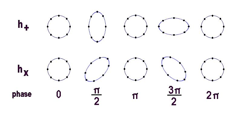
Figure A.1: Ring of particles reacting to the gravitational wave income. Top: $+$ mode, bottom: $\times$ mode.

A.4 Detection of gravitational waves

To specialise the situation of detection [71], suppose we have free, unconstrained masses at two points along the $\hat{x}$ axis separated by a distance $L$. Measuring a local acceleration between these masses relies in the ability of shooting light between them measuring the elapsed time. As if it were a problem in geometric optics, for a light ray connecting the two masses, due to the light-like nature of photons, we have:

$$\operatorname{d}\tau^{2}=g_{\mu\nu}\operatorname{d}x^{\mu}\operatorname{d}x^{\nu}=0\,.$$ (A.43)

As stated in the previous sections, the nature of a gravitational perturbation of the kind similar to a gravity wave far from the source is an extremely weak phenomenon, we can therefore assume again $g_{\mu\nu}=\eta_{\mu\nu}+h_{\mu\nu}$. Under these assumptions, a GW coming from the $\hat{z}$ direction will perturb the metric as the world-line of photons gets distorted as follows:

$$0=\operatorname{d}\tau^{2}=-c^{2}\operatorname{d}t^{2}+(1+h_{11}(\omega t-kz))\operatorname{d}x^{2}\,,$$ (A.44)

where now $x$ designates the former $x_{1}$ space coordinate, $c$ is the speed of light in vacuo and the wave vector has been properly chosen, with frequency $\omega$. The effect of the GW is to modulate the distance between the two fixed coordinate points marked by the two masses, by the fractional amount $h_{11}$. The travel time is given by integrating (A.44) over the distance $L$:

$$\int_{0}^{T_{out}}\operatorname{d}t=\frac{1}{c}\int_{0}^{L}\sqrt{1+h_{11}(\omega t-kz)}\operatorname{d}x\,.$$ (A.45)

A similar expression can be written fro the return trip:

$$\int_{T_{out}}^{T}\operatorname{d}t=-\frac{1}{c}\int_{L}^{0}\sqrt{1+h_{11}(\omega t-kz)}\operatorname{d}x\,,$$ (A.46)

and the total round trip is thus

$$T=\frac{2L}{c}+\frac{1}{c}\int_{0}^{L}h_{11}(\omega t-kz)\operatorname{d}x\,,$$ (A.47)

where the expansion $\sqrt{1+x}\simeq 1+\frac{1}{2}x$ was used, having $|h_{11}|\ll 1$.

If timescales are such that $T$ is short compared with the period of the wave we find that the fluctuation in $T$ due to the wave is given by

$$\Delta T=\frac{L}{c}h_{11}\,,$$ (A.48)

or the effective percent change in separation of the masses is

$$\frac{\Delta L}{L}=\frac{h_{11}}{2}\,,$$ (A.49)

therefore $h$ can be interpreted as a physical strain in space.

The former deduction has been carried on bearing in mind $T$ to be larger than the GW period and assuming perfect positioning of the detector with regard to the angular position of the source. For cross polarisation a detector with two masses on a joining line tilted by and angle $\theta$ toward the $\hat{z}$ direction of the incoming wave, with projection on the $\hat{x}-\hat{y}$ plane rotated by $\phi$ with respect to $\hat{x}$, the effective strain will be $h_{11}\sin^{2}\theta\cos 2\phi$.

The scaling law (A.49) won’t hold for arbitrary long interferometer arms [73]. If the optical path is so long that $\omega_{\text{GW}}T\ll 1$ is no longer valid, we have to carry out carefully the integrations in (A.45) and (A.46) considering the “zeroes” of the wave, such that $\omega_{\text{GW}}T=1$: in these cases the light spends exactly one gravitational wave period in the apparatus, for every part of its path for which the light crosses through a region of positive $h$, there’s an equal part for which it sees an equal but opposite value of $h$. Hence no net modulation of the total optical path could be sensed. We need then do drop our assumption of constancy of $h$ along $T$. The easiest way is to think $h(t)$ a modulated plane wave, where $h(t)$ is now slowly varying with respect to $\omega_{\text{GW}}$:

$$h(t)\to h(t)\exp\left(\iota\omega_{\text{GW}}t\right)\,,$$ (A.50)

then the ongoing-path integral can be computed as follows:

$$\int_{0}^{T_{out}}\operatorname{d}t\simeq\frac{L}{c}+\frac{h(t)}{2\iota\omega_{\text{GW}}}\left(\exp\left(\iota\frac{\omega_{\text{GW}}L}{c}\right)-1\right)\,,$$ (A.51)

while the return trip yields

$$\int_{T_{out}}^{T}\operatorname{d}t\simeq\frac{L}{c}+\frac{h(t)}{2\iota\omega_{\text{GW}}}\exp\left(\iota\frac{2\omega_{\text{GW}}L}{c}\right)\left(1-\exp\left(-\iota\frac{\omega_{\text{GW}}L}{c}\right)\right)\,,$$ (A.52)

we thus find, for the time difference, expressed in terms of lengths now, that:

$$\Delta T=\frac{\Delta L}{c}=h(t)\frac{L}{c}\exp\left(-\iota\frac{\omega_{\text{GW}}L}{c}\right)\frac{\sin\left(\frac{\omega_{\text{GW}}L}{c}\right)}{\frac{L}{c}\omega_{\text{GW}}}\,,$$ (A.53)

so that

$$\frac{\Delta L}{L}=h(t)\exp\left(-\iota\frac{\omega_{\text{GW}}L}{c}\right)\operatorname{sinc}\left(\frac{\omega_{\text{GW}}L}{c}\right)\,,$$ (A.54)

where we defined $\operatorname{sinc}x=\nicefrac{{\sin x}}{{x}}$, and it’s easy to see that the result is continuous into the naîve expression (A.49) for $\omega_{\text{GW}}T\ll 1$.

An example of the kind of frequencies at play may be given considering the emission of GW by a binary system in circular orbit. If the two stars are considered to have both mass $m$ and keep orbiting at distance $l$, we can write the force between them as:

$$G\frac{m^{2}}{l^{2}}=m\omega^{2}\frac{l}{2}\,,\quad\text{with}\quad\omega^{2}=\frac{2Gm}{l^{3}}.$$ (A.55)

The energy density is then

$$T^{00}=\sum_{j=1}^{2}mc^{2}\delta(x-x_{j})\delta(y-y_{j})\delta{z}\,,$$ (A.56)

where we considered the stars to be point-like and the orbit lying on the plane $z=0$. The coordinates are dictated by the equations of motion:

$$\begin{cases}x_{1}=\frac{l}{2}\cos\omega t\\ y_{1}=\frac{l}{2}\sin\omega t\end{cases}\quad\begin{cases}x_{2}=-x_{1}\\ y_{2}=-y_{1}\end{cases}\,.$$ (A.57)

After some pain - not so much indeed - all the components of $q_{ij}$ and $Q_{ij}$ can be computed, transposed into TT-gauge and we finally find:

$$h^{TT}_{xx}=-h^{TT}_{yy} =-\frac{G}{2c^{4}r}ml^{2}(2\omega)^{2}\cos 2\omega\left(\frac{r}{c}-t\right)\,,$$ (A.58)

$$h^{TT}_{xy} =\frac{G}{2c^{4}r}ml^{2}(2\omega)^{2}\sin 2\omega\left(\frac{r}{c}-t\right)\,,$$ (A.59)

showing the radiation is emitted at twice the orbital frequency, carries both polarisation and in the specific case it’s circularly polarised.

Observational evidence of the theoretical prediction can be provided by many systems; we choose here the binary pulsar PSR $1913+16$, observed by Taylor and Weisberg in 1982 [74, 75]. From the data it appears $M_{1}\sim M_{2}\sim 1.4M_{\odot}$ and $l\simeq 0.19\times 10^{9}\,m\simeq 2R_{\odot}$, where $M$ designate masses, $R$ whenever used radius’s and the symbol $\odot$ has been employed to name the Sun.

Again from observed data we see the orbit shows some eccentricity (factor $\epsilon=0.62$) but we can assume it’s circular since we are only interested in estimates. The orbital frequency is $\omega\sim 3.7\times 10^{-5}\,\mathrm{Hz}$, so that the wavelength of the emitted GW will be:

$$\lambda_{\text{GW}}=\frac{c}{2\omega}\sim 10^{12}\,\mathrm{m}\,.$$ (A.60)

Indeed, $\lambda_{\text{GW}}\ll l$.

The distance of the system from the Earth if $r=5\,\mathrm{kpc}=1.5\times 10^{20}\,\mathrm{m}$, resulting in a wave amplitude like:

$$\frac{G}{2c^{4}r}ml^{2}(2\omega)^{2}\sim 5.8\times 10^{-23}\,.$$ (A.61)

Another example may be the PSR J0737-3039 pulsar, more eccentric in the orbit and with diversely weighting stars. The estimated amplitude is $h=1.1\times 10^{-21}$, for GW emitted at frequency $\omega_{\text{GW}}=2.3\times 10^{-4}\,\mathrm{Hz}$: this may be a very good candidate for LISA.

As shown, the first experimental problem connected to the detection of GW is the extreme smallness of of predicted amplitudes and strains in the vicinity of the Earth. The weakness of the signal makes it mandatory to reduce the noise - from any source - to minimum. For signals above $\sim 10\,\mathrm{Hz}$, ground based experiments are possible, but for lower frequencies local fluctuating gravitational gradients become important and seismic noise is more problematic, hence detectors for operation in space may be more suitable if not the unique chance to detect GW. An overview of the characteristic frequencies with dependence of the sources is shown in picture A.2 and table 1.1.

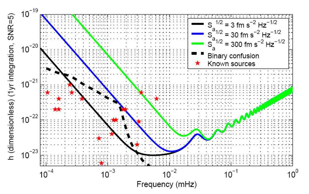
Figure A.2: Strain sensitivity versus known sources for three values of instrumental resolution. Values for sources can be found in table 1.1.

A detailed analysis of noise sources, reduction and subtraction will be placed in the appropriate section.

Let’s give an idea about sensitivity and magnitudes. If we were to build a gravitational wave observatory we could consider test bodies separated by some distance of the order of kilometres. Suppose the incoming wave would have a magnitude $h\simeq 10^{-21}$, then the sensitivity would be of the order

$$\Delta L\simeq 10^{-16}\frac{h}{10^{-21}}\frac{L}{\mathrm{km}}\,\mathrm{cm}\,,$$ (A.62)

comparable with the size of atoms $a_{0}\simeq 5\times 10^{-11}\,\mathrm{m}$. A gravitational wave observatory will have to be sensitive to changes in distances much smaller than the size of the constituent atoms out of which the masses have to be made.

Laser interferometers provide a way to perform such an accurate measurement.

Appendix B Basic facts in differential geometry

In support to chapter 1, this appendix is meant to review some basic concepts of differential geometry with the purpose of defining parallel transporters and geodesics, both in absence and in presence of external forces.

The geodesics mutual acceleration equation and its link to the Riemann tensor is reviewed in the general case and in weak field approximation.

We’ll provide some text-book based demonstrations at need, which may please the mathematically skilled reader. We invite anyway to get to a more advanced exposition (books and cited articles) if need were for finer details.

B.1 Geodesics

According to differential geometry a geodesic is a curve defined by a parallel transporter along itself. The curve may be thought as a single parameter string $C=C(\tau)=\left\{x^{\mu}(\tau),\,\mu=0..3\right\}$, so that its tangent vector component $V^{\mu}$ con be easily obtained as [69, 16]:

$$V^{\mu}=\frac{\operatorname{d}x^{\mu}}{\operatorname{d}\tau}\,.$$ (B.1)

Parallel transport along the tangent vector ${\boldsymbol{V}}$ is put in place by means of the parallel transport operator $\nabla_{{\boldsymbol{V}}}$. Naturally, when parallel transporting a vector along itself, we have no variation of trajectory:

$$\nabla_{{\boldsymbol{V}}}{\boldsymbol{V}}=0\,,$$ (B.2)

where

$$\left(\nabla_{{\boldsymbol{V}}}{\boldsymbol{X}}\right)^{\mu}=V^{\alpha}X^{\mu}_{\phantom{\mu};\alpha}=V^{\alpha}\left(X^{\mu}_{\phantom{\mu},\alpha}+\Gamma^{\mu}_{\phantom{\mu}\alpha\beta}X^{\beta}\right)\,.$$ (B.3)

We used the comma to designate standard partial derivative: $X^{\mu}_{\phantom{\mu},\alpha}=\partial_{\alpha}X^{\mu}$ while the semicolon abbreviates the standard co-variant one. Christoffel symbols bearing affine connection are related to the metric as follows:

$$\Gamma^{\rho}_{\phantom{\rho}\mu\nu}=\frac{1}{2}g^{\rho\sigma}\left(g_{\nu\sigma,\mu}+g_{\mu\sigma,\nu}-g_{\mu\nu,\sigma}\right)\,.$$ (B.4)

As a side remark, notice the connection symbols may be not related to a proper metric tensor, the transport equation being general in nature.

By substitution of the expression of $V^{\mu}$, the geodesic equation reads:

$$0=\nabla_{{\boldsymbol{V}}}{\boldsymbol{V}} =V^{\alpha}\left(V^{\mu}_{\phantom{\mu},\alpha}+\Gamma^{\mu}_{\phantom{\mu}\alpha\beta}V^{\beta}\right)=$$ (B.5)

$$=\frac{\operatorname{d}x^{\alpha}}{\operatorname{d}\tau}\partial_{\alpha}\frac{\operatorname{d}x^{\mu}}{\operatorname{d}\tau}+\Gamma^{\mu}_{\phantom{\mu}\alpha\beta}\frac{\operatorname{d}x^{\alpha}}{\operatorname{d}\tau}\frac{\operatorname{d}x^{\beta}}{\operatorname{d}\tau}=$$ (B.6)

$$=\frac{\operatorname{d}^{2}x^{\alpha}}{\operatorname{d}\tau^{2}}+\Gamma^{\mu}_{\phantom{\mu}\alpha\beta}\frac{\operatorname{d}x^{\alpha}}{\operatorname{d}\tau}\frac{\operatorname{d}x^{\beta}}{\operatorname{d}\tau}\,,$$ (B.7)

where we used

$$\frac{\operatorname{d}x^{\alpha}}{\operatorname{d}\tau}\partial_{\alpha}\frac{\operatorname{d}x^{\mu}}{\operatorname{d}\tau}=\frac{\operatorname{d}x^{\alpha}}{\operatorname{d}\tau}\frac{\partial\tau}{\partial x^{\alpha}}\frac{\operatorname{d}}{\operatorname{d}\tau}\frac{\operatorname{d}x^{\mu}}{\operatorname{d}\tau}=\frac{\operatorname{d}^{2}x^{\mu}}{\operatorname{d}\tau^{2}}\,.$$ (B.8)

Then, there’s no acceleration along a geodesic on the line flow dictated by the natural parameter, i.e. the pure parallel motion is indeed “freely falling”.

B.2 External forces. $3+1$ representation

In presence of an external disturbance both EM and generic the geodesics equation gets modified as follows:

$$\frac{\operatorname{d}^{2}x^{\mu}}{\operatorname{d}\tau^{2}}+\Gamma^{\mu}_{\phantom{\mu}\alpha\beta}\frac{\operatorname{d}x^{\alpha}}{\operatorname{d}\tau}\frac{\operatorname{d}x^{\beta}}{\operatorname{d}\tau}=\frac{e}{m}F^{\mu}_{\phantom{\mu}\sigma}\frac{\operatorname{d}x^{\sigma}}{\operatorname{d}\tau}+\frac{1}{m}f^{\mu}\,,$$ (B.9)

where $F_{\mu\nu}=A_{\mu,\nu}-A_{\nu,\mu}=A_{[\mu,\nu]}$ and $A_{\mu}$ is the usual EM $4$-potential such that the fields can be calculated as $E_{i}=A_{0,i}$ and $B_{i}=\epsilon_{ijk}A_{j,k}$. $e$ is the electron charge and $m$ is the mass of the test-body at play.

In general:

$$a^{i}=\frac{\operatorname{d}^{2}x^{i}}{\operatorname{d}t^{2}}=\left(\frac{\operatorname{d}\tau}{\operatorname{d}t}\right)^{2}\left(\frac{\operatorname{d}^{2}x^{i}}{\operatorname{d}\tau^{2}}-v^{i}\frac{\operatorname{d}^{2}t}{\operatorname{d}\tau^{2}}\right)\,,$$ (B.10)

where $v^{i}=\nicefrac{{\operatorname{d}x^{i}}}{{\operatorname{d}t}}$. substituting from the geodesic equation we get:

$$\frac{\operatorname{d}^{2}x^{i}}{\operatorname{d}t^{2}}=\left(\frac{\operatorname{d}\tau}{\operatorname{d}t}\right)^{2}\left(-\Gamma^{i}_{\phantom{\mu}\alpha\beta}\frac{\operatorname{d}x^{\alpha}}{\operatorname{d}\tau}\frac{\operatorname{d}x^{\beta}}{\operatorname{d}\tau}-v^{i}\frac{\operatorname{d}^{2}t}{\operatorname{d}\tau^{2}}\right)\,,$$ (B.11)

together with

$$\frac{\operatorname{d}^{2}t}{\operatorname{d}\tau^{2}}=-\Gamma^{0}_{\phantom{\mu}\alpha\beta}\frac{\operatorname{d}x^{\alpha}}{\operatorname{d}\tau}\frac{\operatorname{d}x^{\beta}}{\operatorname{d}\tau}\,.$$ (B.12)

Employing the chain rule we can use $\frac{\operatorname{d}x^{\alpha}}{\operatorname{d}\tau}=\frac{\operatorname{d}x^{\alpha}}{\operatorname{d}t}\frac{\operatorname{d}t}{\operatorname{d}\tau}$ so that the l.h.s. of (B.9) can be expressed recast in $3+1$ representation with the time $t$ as independent variable:

$$\frac{\operatorname{d}^{2}x^{i}}{\operatorname{d}t^{2}}=\left(-\Gamma^{i}_{\phantom{i}00}-2\Gamma^{i}_{\phantom{i}0j}v^{j}-\Gamma^{i}_{\phantom{i}jk}v^{j}v^{k}+v^{i}\left(\Gamma^{0}_{\phantom{0}00}+2\Gamma^{0}_{\phantom{i}0j}v^{j}+\Gamma^{0}_{\phantom{i}jk}v^{j}v^{k}\right)\right)\,,$$ (B.13)

Of course, this is not the case if local forces act on the couple of particles. In this case, the tidal terms on r.h.s. of the acceleration equation pick up corrections of the following form

$$\frac{e}{m}\left(F^{i}_{\phantom{i}\sigma}v^{\sigma}-F^{0}_{\phantom{0}j}v^{j}v^{i}\right)\frac{\operatorname{d}\tau}{\operatorname{d}t}+\frac{1}{m}\left(f^{i}-f^{0}v^{i}\right)\left(\frac{\operatorname{d}\tau}{\operatorname{d}t}\right)^{2}\,.$$ (B.14)

If the velocities are small ($|v^{i}|\ll 1$), we get then

$$\frac{\operatorname{d}^{2}t}{\operatorname{d}\tau^{2}}\simeq 0\quad\Rightarrow\quad\frac{\operatorname{d}t}{\operatorname{d}\tau}\simeq\text{const.}\,$$ (B.15)

but if the velocities are small it is also geometrically true that

$$\operatorname{d}\tau^{2}=g_{\mu\nu}\operatorname{d}x^{\mu}\operatorname{d}x^{\nu}\simeq g_{00}\operatorname{d}t^{2}\,,$$ (B.16)

hence

$$\operatorname{d}t\simeq\frac{\operatorname{d}\tau}{\sqrt{g_{00}}}=\frac{\operatorname{d}\tau}{\sqrt{\eta_{00}+h_{00}}}\simeq\operatorname{d}\tau$$ (B.17)

and finally the true deviations at small velocities are given by

$$\frac{e}{m}\left(F^{i}_{\phantom{i}0}+F^{i}_{\phantom{i}k}v^{k}\right)+\frac{1}{m}\left(f^{i}-f^{0}v^{i}\right)\,.$$ (B.18)

At low velocities then, with no assumptions whatsoever on the form of the metric tensor, we are brought to the expression of local accelerations in real time (notice we drop the terms quadratic in the velocities):

$$\frac{\operatorname{d}^{2}x^{i}}{\operatorname{d}t^{2}}=\left(-\Gamma^{i}_{\phantom{i}00}-2\Gamma^{i}_{\phantom{i}0j}v^{j}+\Gamma^{0}_{\phantom{0}00}v^{i}\right)+e\left(F^{i}_{\phantom{i}0}+F^{i}_{\phantom{i}k}v^{k}\right)+\left(f^{i}-f^{0}v^{i}\right)+O(v^{2})\,.$$ (B.19)

B.3 Congruence of geodesics. Geodesics deviation

If the curves form a set, they can be parametrised or indexed by a continuous parameter $\sigma$, hence a second vector acquires meaning, describing the motion orthogonal to the geodesics:

$$W^{\mu}=\frac{\operatorname{d}x^{\mu}}{\operatorname{d}\sigma}\,.$$ (B.20)

We proceed now to calculate the Lie derivative of ${\boldsymbol{W}}$ along ${\boldsymbol{V}}$:

$${\mathcal{L}}_{{\boldsymbol{V}}}W^{\mu} =V^{\alpha}W^{\mu}_{\phantom{\mu},\alpha}-W^{\alpha}V^{\mu}_{\phantom{\mu},\alpha}=$$ (B.21)

$$=\frac{\operatorname{d}x^{\alpha}}{\operatorname{d}\tau}\partial_{\alpha}\frac{\operatorname{d}x^{\mu}}{\operatorname{d}\sigma}-\frac{\operatorname{d}x^{\alpha}}{\operatorname{d}\sigma}\partial_{\alpha}\frac{\operatorname{d}x^{\mu}}{\operatorname{d}\tau}=$$ (B.22)

$$=\frac{\operatorname{d}^{2}x^{\mu}}{\operatorname{d}\tau\operatorname{d}\sigma}-\frac{\operatorname{d}^{2}x^{\mu}}{\operatorname{d}\sigma\operatorname{d}\tau}=0$$ (B.23)

on the other hand

$${\mathcal{L}}_{{\boldsymbol{V}}}W^{\mu} =V^{\alpha}W^{\mu}_{\phantom{\mu},\alpha}-W^{\alpha}V^{\mu}_{\phantom{\mu},\alpha}+\Gamma^{\mu}_{\phantom{\mu}\alpha\beta}\left(V^{\alpha}W^{\beta}-V^{\beta}W^{\alpha}\right)=$$ (B.24)

$$=V^{\alpha}W^{\mu}_{\phantom{\mu};\alpha}-W^{\alpha}V^{\mu}_{\phantom{\mu};\alpha}=$$ (B.25)

$$=\nabla_{{\boldsymbol{V}}}W^{\mu}-\nabla_{{\boldsymbol{W}}}V^{\mu}\,,$$ (B.26)

since $\Gamma^{\mu}_{\phantom{\mu}\alpha\beta}=\Gamma^{\mu}_{\phantom{\mu}\beta\alpha}$.

We showed that

$$\nabla_{{\boldsymbol{V}}}W^{\mu}=\nabla_{{\boldsymbol{W}}}V^{\mu}$$ (B.27)

and then

$$\nabla_{{\boldsymbol{V}}}\nabla_{{\boldsymbol{W}}}V^{\mu}=\nabla_{{\boldsymbol{V}}}\nabla_{{\boldsymbol{V}}}W^{\mu}\,,$$ (B.28)

therefore, the latter expression gives the relative, co-variant acceleration of the separation vector between geodesics.

We now wish to calculate:

$$\nabla_{{\boldsymbol{[}}V}\nabla_{{\boldsymbol{W}}]}V^{\mu}=\nabla_{{\boldsymbol{V}}}\nabla_{{\boldsymbol{W}}}V^{\mu}-\nabla_{{\boldsymbol{W}}}\nabla_{{\boldsymbol{V}}}V^{\mu}\,$$ (B.29)

by using $\nabla_{{\boldsymbol{V}}}V^{\mu}=0$ and $\nabla_{{\boldsymbol{V}}}\nabla_{{\boldsymbol{W}}}V^{\mu}=\nabla_{{\boldsymbol{V}}}\nabla_{{\boldsymbol{V}}}W^{\mu}$ and relate it to the former acceleration.

We have:

$$\nabla_{[{\boldsymbol{V}}}\nabla_{{\boldsymbol{W}}]}V^{\mu}=$$ (B.33)

$$= \nabla_{{\boldsymbol{V}}}\nabla_{{\boldsymbol{W}}}V^{\mu}=$$ (B.34)

$$= V^{\alpha}\left(W^{\beta}V^{\mu}_{\phantom{\mu};\beta}\right)_{;\alpha}=V^{\alpha}W^{\beta}_{\phantom{\beta};\alpha}V^{\mu}_{\phantom{\mu};\beta}+V^{\alpha}W^{\beta}V^{\mu}_{\phantom{\mu};\beta;\alpha}=$$ (B.35)

$$= W^{\alpha}V^{\beta}_{\phantom{\beta};\alpha}V^{\mu}_{\phantom{\mu};\beta}+V^{\alpha}W^{\beta}\left(V^{\mu}_{\phantom{\mu};\alpha;\beta}+R^{\mu}_{\phantom{\mu}\nu\alpha\beta}V^{\nu}\right)=$$ (B.36)

$$= W^{\alpha}V^{\beta}_{\phantom{\beta};\alpha}V^{\mu}_{\phantom{\mu};\beta}+W^{\beta}\left(V^{\alpha}V^{\mu}_{\phantom{\mu};\alpha}\right)_{;\beta}-W^{\beta}V^{\alpha}_{\phantom{\mu};\beta}V^{\mu}_{\phantom{\mu};\alpha}+W^{\beta}V^{\alpha}R^{\mu}_{\phantom{\mu}\nu\alpha\beta}V^{\nu}=$$ (B.37)

$$= R^{\mu}_{\phantom{\mu}\nu\beta\alpha}V^{\nu}V^{\beta}W^{\alpha}\,.$$ (B.38)

Finally:

$$\nabla_{{\boldsymbol{V}}}\nabla_{{\boldsymbol{V}}}W^{\mu}=R^{\mu}_{\phantom{\mu}\nu\beta\alpha}V^{\nu}V^{\beta}W^{\alpha}\,.$$ (B.39)

B.4 Further developments. Geodesics deviation equation at low speed

By means of eq. (B.28) and the definition of geodesic the latter result can be written also in the following form [15, 76]:

$$\ddot{W}^{\mu}=-\Gamma^{\mu}_{\phantom{\mu}\beta\alpha}\dot{W}^{\alpha}\dot{W}^{\beta}+R^{\mu}_{\phantom{\mu}\nu\beta\alpha}V^{\nu}V^{\beta}W^{\alpha}\,,$$ (B.40)

where now $\dot{W}^{\mu}\equiv\operatorname{d}W^{\mu}/\operatorname{d}\tau$. After some simplifications, we get:

$$\ddot{W}^{\mu}=-\Gamma^{\mu}_{\phantom{\mu}\beta\alpha,\gamma}V^{\beta}V^{\alpha}W^{\gamma}-2\Gamma^{\mu}_{\phantom{\mu}\beta\alpha}V^{\beta}\dot{W}^{\alpha}\,.$$ (B.41)

Notice there’s no contradiction between the different forms, since we can always choose the origin of connection so to make it vanish in the neighbourhood of the origin itself. Hence the second term of (B.41) would vanish, and the Riemann tensor would simplify til getting the simple form:

$$R^{\mu}_{\phantom{\mu}\nu\beta\alpha}=\Gamma^{\mu}_{\phantom{\mu}\nu\alpha,\beta}-\Gamma^{\mu}_{\phantom{\mu}\nu\beta,\alpha}\,,$$ (B.42)

and the first term of the latter may always be made $0$ along the whole geodesic in the first place but even more simply just proper-time to proper-time.

Taking now (B.41) and evaluating it in TT-gauge, i.e. with the choices:

$$\Gamma^{i}_{\phantom{i}00}=\Gamma^{0}_{\phantom{0}00}=\Gamma^{0}_{\phantom{0}0j} =0\,,$$ (B.43)

$$\Gamma^{0}_{\phantom{0}jk}=\frac{1}{2}\eta^{0\nu}\left(h_{\nu j,k}+h_{k\nu,j}-h_{jk,\nu}\right) =-\frac{1}{2}h_{jk,0}\,.$$ (B.44)

$$\Gamma^{i}_{\phantom{i}0j}=\frac{1}{2}\eta^{i\nu}\left(h_{\nu 0,j}+h_{j\nu,0}-h_{0j,\nu}\right) =\frac{1}{2}h_{j\phantom{i},0}^{\phantom{j}i}\,,$$ (B.45)

we are left with:

$$\begin{split}\ddot{W}^{0}&=-\Gamma^{0}_{\phantom{0}ij,\gamma}V^{i}V^{j}W^{\gamma}-2\Gamma^{0}_{\phantom{0}ij}V^{i}\dot{W}^{j}\,,\\ \ddot{W}^{i}&=-\Gamma^{i}_{\phantom{i}0j,\gamma}V^{0}V^{j}W^{\gamma}-2\Gamma^{i}_{\phantom{i}0j}V^{0}\dot{W}^{j}\,.\end{split}$$ (B.46)

Assume that now initially $V^{\alpha}=\delta^{\alpha}_{\phantom{\alpha}0}+O(h)$, so that $V^{i}=0\,i=1..3$, we’d get then:

$$\begin{split}\ddot{W}^{0}&\simeq 0\,,\\ \ddot{W}^{i}&\simeq-2\Gamma^{i}_{\phantom{i}0j}\dot{W}^{j}\,,\end{split}$$ (B.47)

and, since we can trade $\tau$ for $t$, we finally get:

$$\frac{\operatorname{d}^{2}W^{i}}{\operatorname{d}t^{2}}\simeq-\dot{h}_{j}^{\phantom{j}i}\frac{\operatorname{d}W^{j}}{\operatorname{d}t}\,,$$ (B.48)

to order $h$. This result is in contrast to what all standard textbooks claim. In fact, the usual result:

$$\frac{\operatorname{d}^{2}W^{i}}{\operatorname{d}t^{2}}\simeq\frac{1}{2}\ddot{h}_{j}^{\phantom{j}i}W^{j}\,,$$ (B.49)

is derived from (B.39) under the assumption that $\Gamma^{\mu}_{\phantom{\mu}\beta\alpha,\gamma}V^{\gamma}=\dot{\Gamma}^{\mu}_{\phantom{\mu}\beta\alpha}=0$, so that $\nabla_{{\boldsymbol{V}}}\nabla_{{\boldsymbol{V}}}W^{\mu}=\ddot{W}^{\mu}$, but with this very same argument then we’d get $\ddot{W}^{i}=0$ rather then (B.49). In practise, (B.49) is apparently inconsistent with the Transverse-Traceless gauge condition [76]. Notice smoke clears and the two equations convey no contradiction if one points out that (B.49) is derived from the gauge-invariant expression (B.39) in the proper reference frame of the detector, while (B.48) holds in the Lorentz frame of the waves themselves: therefore we have to rely in (B.49) due to its gauge-invariant nature in our reference frame to detect effects of GWs, but and observer sitting on the GWs would conclude by virtue of (B.48) that no effect is produced by the waves.

Appendix C Conclusions

Starting this work we listed some problems and issues which needed some clarification on the LTP and LISA projects. Up to a certain level we reduced the extension of some of these and others were - we think - completely solved:

1. the problem of a construction of a TT-gauged frame was shown to be solvable by an ensemble of tetrads co-moving with the laser beam. Thus, a one-to-one map is built between the perturbed metric change in space-time and the laser phase;

2. the problem of building signals out of a complicated dynamics and selecting a MBW to guarantee correct estimation of a differential acceleration observable was addressed;

3. gravitational static unbalance was analysed and a global numerical strategy based on local multipole expansion elucidated;

4. calibration of force-to-displacement actuation was successfully addressed and the method of Wiener-Kolmogorov proven to be a correct strategy for the task;

5. the problem of charge collection and estimation on the TM surface was tackled in many ways;

6. cross-talk was reduced to its main causes, the effect carried onto the relevant signals and estimated throughout the whole MBW on the basis of up-to-date specifications.

A number of open issues emanate from the former successes:

1. further analyses of static gravity with modified ISL dynamics shall be carried on to test LTP ability to perform an ISL test;

2. all the remaining operation procedures described in chapter 4 which were not deeply inspected (as the charge measurement or the calibration of force to displacement) shall be analysed carefully.

3. LTP may very well fail in some of the more advanced tasks we listed in chapter 4, but the simple residual acceleration noise picture across some integration time can be guaranteed a result provided no problem in releasing the TMs will occur and laser metrology won’t be damaged. Adherence problems are now being addressed with new experimental apparata and more tests will be performed on the caging mechanism.

We hope we convinced the reader of the reliability of LTP, both from the point of view of the theory and as an experimental device. If points were left pending and may seem obscure, we may take the blame of it as little scientific communicators, perhaps. The time needed by two PhD’s courses in sequence won’t be enough to enter all the intricacies of the experiment - at least from our standing position as junior scientists. If we were allowed to abuse a statement, that will be Kant’s “I can, therefore I must”; we contributed to showing that LTP will work, this measure can be done, hence we must do it.

We wish long life to LTP, to serve its purpose for LISA, and we really hope it will bring unexpected news from space.

Appendix D Colophon

[Omissis]

Appendix E Homage

References

- [1] D. Alighieri, La divina commedia, vol. 1. La Nuova Italia Editrice, comm. sapegno, n. ed., 1982.
- [2] L. Ricci, “Dante’s insight into galilean invariance,” Nature 434 (2005) no. 434, 717.
- [3] N. Copernico, De revolutionibus orbium caelestium. Einaudi, einaudi, 1975 ed., 1543.
- [4] A. Einstein, “Die Grundlage der allgemeinen Relativitätstheorie,” Annalen der Physik 49 (1916) 769–822.
- [5] E. Einstein, H. A. Lorentz, H. Weyl, and H. Minkowski, The principle of relativity. Dover, 1952.
- [6] Merriam-Webster, Merriam-webster’s collegiate dictionary. Merriam-Webster, 11th ed., July, 2003.
- [7] M. Armano, D. Bortoluzzi, C. D. Hoyle, and S. Vitale, “Gravitational compensation for the LISA pathfinder,” Class. Quant. Grav. 22 (2005) S501–S507. http://dx.doi.org/10.1088/0264-9381/22/10/050.
- [8] M. Armano, D. Bortoluzzi, and S. Vitale, “LTP gravitation control protocol,” LTPA-UTN iss001-rev1, University of Trento, March, 15, 2004.
- [9] M. Armano and S. Vitale, “Note on cross-talk measurements on LISA-PF,” S2-UTN TN-3008, University of Trento, March 1, 2005.
- [10] S. Anza, M. Armano, E. Balaguer, M. Benedetti, C. Boatella, P. Bosetti, D. Bortoluzzi, N. Brandt, C. Braxmaier, M. Caldwell, L. Carbone, A. Cavalleri, A. Ciccolella, I. Cristofolini, M. Cruise, M. Da Lio, K. Danzmann, D. Desiderio, R. Dolesi, N. Dunbar, W. Fichter, C. Garcia, E. Garcia-Berro, A. F. Garcia Marin, R. Gerndt, A. Gianolio, D. Giardini, R. Gruenagel, A. Hammesfahr, G. Heinzel, J. Hough, D. Hoyland, M. Hueller, O. Jennrich, U. Johann, S. Kemble, C. Killow, D. Kolbe, M. Landgraf, A. Lobo, V. Lorizzo, D. Mance, K. Middleton, F. Nappo, M. Nofrarias, G. Racca, J. Ramos, D. Robertson, M. Sallusti, M. Sandford, J. Sanjuan, P. Sarra, A. Selig, D. Shaul, D. Smart, M. Smit, L. Stagnaro, T. Sumner, C. Tirabassi, S. Tobin, S. Vitale, V. Wand, H. Ward, W. J. Weber, and P. Zweifel, “The LTP experiment on the LISA pathfinder mission,” Class. Quant. Grav. 22 (2005) S125–S138. http://www.iop.org/EJ/abstract/0264-9381/22/10/001.
- [11] N. Tateo, “System identification nel processo di misura, calibrazione e filtraggio dei segnali della missione LISA/LTP,” Master’s thesis, Politecnico di Milano - Dipartimento di Ingegneria Aerospaziale, 2006.
- [12] M. Armano, K. Danzmann, R. Dolesi, A. Garcia Marin, G. Heinzel, M. Hueller, S. Vitale, and W. Weber, “LTP experiments master plan,” tech. rep., University of Trento, Albert Einstein Institut Hannover, March 1, 2005.
- [13] S. Vitale, “Data analysis requirement document,” S2-UTN RS-3001, University of Trento, May 27, 2006.
- [14] R. Dolesi et al., “Gravitational sensor for LISA and its technology demonstration mission,” Class. Quant. Grav. 20 (2003) S99–S108.
- [15] S. Weinberg, Gravitation and cosmology, principles and applications of the general theory of relativity. Wiley, 1972.
- [16] R. d’Inverno, Introducing Einstein’s Relativity. Oxford University Press, 1992.
- [17] P. Olesen and J. Ambjoern, General relativity, cosmology and classical gauge theories. University of Copenhagen, The Niels Bohr Institute, 1999-2000.
- [18] K. S. Thorne, “Multipole expansions of gravitational radiation,” Rev. Mod. Phys. 52 (1980) 299–339.
- [19] C. Misner, K. S. Thorne, and J. A. Wheeler, Gravitation. W.H. Freeman and Company, San Francisco, 1973.
- [20] S. A. Teukolsky, “Linearized quadrupole waves in general relativity and the motion of test particles,” Phys. Rev. D26 (1982) 745–750.
- [21] D. Garfinkle, “Gauge invariance and the detection of gravitational radiation,” arXiv (2005) .
- [22] L. Carbone et al., “Achieving geodetic motion for LISA test masses: Ground testing results,” Phys. Rev. Lett. 91 (2003) 151101, gr-qc/0307008.
- [23] L. Carbone, Ground based investigation of force noise sources for LISA. PhD thesis, University of Trento, 2005.
- [24] T. J. Sumner and D. N. A. Shaul, “The observation of gravitational waves from space using LISA,” Mod. Phys. Lett. A19 (2004) 785–800.
- [25] S. Vitale, K. Danzmann, et al., “LISA technology package architect the LISA technology package on board smart-2,” Tech. Rep. LTPA-UTN-Int-10.2002-rel1.3, University of Trento, Albert Einstein Institut Hannover, University of Birmingham, Carlo Gavazzi Space Italia SPA, SRON, University of Glasgow, IEEC Barcelona, Autonomous University of Barcelona, Imperial College London, University of Urbino, Oct, 2002.
- [26] D. Bortoluzzi, C. D. Hoyle, M. Hueller, S. Vitale, G. Heinzel, K. Danzmann, A. Lobo, S. Anza, C. Navau, C. Du-Xing, A. Sanchez, H. Araujo, P. Wass, and C. Grimani, “Science requirements and top-level architecture definition for the LISA technology package (LTP) on board LISA pathfinder (SMART-2),” LTPA-UTN ScRD-iss003-rev1, UNITN, AEI Hannover, IEEC Barcelona, AU Barcelona, IC London, UNIURB, June 30, 2005.
- [27] S. Vitale et al., “Lisa and its in-flight test precursor smart-2,” Nucl. Phys. Proc. Suppl. 110 (2002) 209–216.
- [28] R. T. Stebbins et al., “Current error estimates for LISA spurious accelerations,” Class. Quant. Grav. 21 (2004) S653–S660.
- [29] L. Carbone et al., “Characterization of disturbance sources for LISA: Torsion pendulum results,” Class. Quant. Grav. 22 (2005) S509–S520, gr-qc/0412103.
- [30] L. Carbone et al., “Improved torsion pendulum for ground testing of LISA displacement sensors,” arXiv (2004) , gr-qc/0411049.
- [31] L. Carbone et al., “Upper limits on stray force noise for LISA,” Class. Quant. Grav. 21 (2004) S611–S620, gr-qc/0310119.
- [32] A. Cavalleri et al., “Progress in the development of a position sensor for LISA drag-free control,” Class. Quant. Grav. 18 (2001) 4133–4144.
- [33] M. Hueller, A. Cavalleri, R. Dolesi, S. Vitale, and W. J. Weber, “Torsion pendulum facility for ground testing of gravitational sensors for LISA,” Class. Quant. Grav. 19 (2002) 1757–1765.
- [34] D. Bortoluzzi et al., “Measuring random force noise for LISA aboard the LISA pathfinder mission,” Class. Quant. Grav. 21 (2004) S573–S580, gr-qc/0402020.
- [35] D. Bortoluzzi et al., “Testing LISA drag-free control with the LISA technology package flight experiment,” Class. Quant. Grav. 20 (2003) S89–S97.
- [36] W. Weber, D. Bortoluzzi, A. Cavalleri, L. Carbone, M. Da Lio, R. Dolesi, G. Fontana, C. Hoyle, M. Hueller, and S. Vitale, “Position sensors for flight testing of LISA drag-free control,” in Gravitational-Wave Detection. Proceedings of the SPIE., M. Cruise and P. Saulson, eds., vol. 4856, pp. 31–42, SPIE. Mar., 2003.
- [37] T. Sumner et al., “Description of charging / discharging processes of the LISA sensors,” Class. Quant. Grav. 21 (2004) S597–S602.
- [38] M. Landgraf, M. Hechler, and S. Kemble, “Mission design for LISA pathfinder,” Class. Quant. Grav. 22 (2005) S487–S492, gr-qc/0411071.
- [39] A. Schleicher, M. Schlotterer, and W. Fichter, “DFACS science mode 1 design and analysis (m3),” S2-ASD TN-2003-iss21, EADS Astrium, January 9, 2006.
- [40] A. Schleicher, M. Schlotterer, and W. Fichter, “DFACS general design,” S2-ASD TN-2001-iss21, EADS Astrium, November 17, 2005.
- [41] A. Schleicher, M. Schlotterer, and W. Fichter, “DFACS functional architecture,” S2-ASD TN-2008-iss1, EADS Astrium, Jun, 2005.
- [42] A. Schleicher, M. Schlotterer, and W. Fichter, “DFACS normal mode design and analysis,” S2-ASD TN-2002-iss21, EADS Astrium, Jan, 2006.
- [43] A. Schleicher and D. Wealthy, “DFACS requirement specification,” Tech. Rep. S2-ASD-RS-2001, EADS Astrium, Jul, 2008.
- [44] W. J. Weber et al., “Position sensors for LISA drag-free control,” Class. Quant. Grav. 19 (2002) 1751–1756.
- [45] M. Armano and S. Vitale, “LTP noise budget,” S2-UTN TN-3030, University of Trento, June 4, 2006.
- [46] D. Bortoluzzi and W. Weber, “Test mass electrostatic suspension actuation stiffness and cross-talk matrix,” S2-UTN TN-3009-draft, University of Trento, March, 2005.
- [47] M. Armano, L. Carbone, A. Cavalleri, R. Dolesi, C. Hoyle, M. Hueller, S. Vitale, and W. Weber, “Measuring the LISA test mass magnetic proprieties with a torsion pendulum,” Class. Quant. Grav. 22 (2005) S521–S526, gr-qc/0412093.
- [48] M. Hueller, Geodesic motion of LISA test masses: Development and testing of drag-free position sensors. PhD thesis, University of Trento, 2003.
- [49] H. B. Callen and T. A. Welton, “Irreversibility and generalized noise,” Phys. Rev. 83 (Jul, 1951) 34–40.
- [50] R. F. Greene and H. B. Callen, “On the formalism of thermodynamic fluctuation theory,” Phys. Rev. 83 (Sep, 1951) 1231–1235.
- [51] C. M. Caves, “Quantum limits on noise in linear amplifiers,” Phys. Rev. D 26 (Oct, 1982) 1817–1839.
- [52] AURIGA Collaboration, A. Vinante, “Present performance and future upgrades of the auriga capacitive readout,” Class. Quant. Grav. 23 (2006) S103–S110.
- [53] F. Acernese et al., “Status of virgo,” Journ. Phys. Conf. Ser. 39 (2006) 32–35.
- [54] A. Roth, Vacuum technology. North-Holland, 1982.
- [55] R. Eisberg and R. Resnick, Quantum physics of atoms, molecules, solids, nuclei, and particles. Wiley, January, 1985.
- [56] S. Vitale, “Calculation of molecular conductance across the test-mass and of the effect of asymmetric outgassing,” tech. rep., University of Trento, January 2003.
- [57] K. Danzmann, P. McNamara, and S. Vitale, “Guidelines for the LTP experiment planning,” S2-UTN TN-3031, University of Trento, 2006.
- [58] C. M. Will, Theory and experiment in gravitational physics. Cambridge University Press, 1993.
- [59] S. Vitale, “Gravitational field compensation,” internal note, UNITN, Nov 2001.
- [60] J. Hanson, G. Keiser, S. Buchman, R. L. Byer, D. Lauben, B. Shelef, G. Shelef, V. Hruby, and M. Gamero-Castano, “Disturbance reduction system: Testing technology for drag-free operation,” vol. 4856, pp. 9–18. SPIE, 2003. http://link.aip.org/link/?PSI/4856/9/1.
- [61] W. M. Folkner, S. Buchman, R. L. Byer, D. B. DeBra, C. J. Dennehy, M. Gamero-Castano, J. Hanson, V. Hruby, G. M. Keiser, A. Kuhnert, F. L. Markley, M. Houghton, P. Maghami, D. C. Miller, S. Prakash, and R. Spero, “Disturbance reduction system: Testing technology for precision formation control,” in Proc. SPIE, A. B. Schultz and R. G. Lyon, eds., vol. 4860, pp. 221–228. SPIE, 2003. http://link.aip.org/link/?PSI/4860/221/1.
- [62] J. Bekenstein and J. Magueijo, “Modified newtonian dynamics habitats within the solar system,”Phys. Rev. D 73 (May, 2006) 103513. http://dx.doi.org/10.1103/PhysRevD.73.103513.
- [63] E. G. Adelberger, N. A. Collins, and C. D. Hoyle, “Analytic expressions for gravitational inner multipole moments of elementary solids and for the force between two rectangular solids,” Class. Quant. Grav. 23 (2006) 125–136, gr-qc/0512055.
- [64] S. S. McGaugh, “Confrontation of mond predictions with wmap first year data,” Astrophys. Journ. 611 (2004) 26–39, astro-ph/0312570.
- [65] J. Bekenstein, “Relativistic gravitation theory for the mond paradigm,” Phys. Rev. D70 (2004) 083509, astro-ph/0403694.
- [66] K. Tangen, “Could the pioneer anomaly have a gravitational origin?,” arXiv (2006) . http://www.citebase.org/cgi-bin/citations?id=oai:arXiv.org:gr-qc/0602089.
- [67] M.-T. Jaekel and S. Reynaud, “Gravity tests and the pioneer anomaly,” arXiv (2005) . http://www.citebase.org/cgi-bin/citations?id=oai:arXiv.org:gr-qc/0511020.
- [68] J. D. Anderson, P. A. Laing, E. L. Lau, A. S. Liu, M. M. Nieto, and S. G. Turyshev, “Indication, from pioneer 10/11, galileo, and ulysses data, of an apparent anomalous, weak, long-range acceleration,” Phys. Rev. Lett. 81 (1998) 2858. http://www.citebase.org/cgi-bin/citations?id=oai:arXiv.org:gr-qc/9808081.
- [69] R. M. Wald, General relativity. The University of Chicago Press, 1984.
- [70] I. Chakrabarty, “Gravitational waves: An introduction,” arXiv (1999) , physics/9908041.
- [71] E. E. Flanagan and S. A. Hughes, “The basics of gravitational wave theory,” New Journ. Phys. 7 (2005) 204.
- [72] D. M. Eardley, D. L. Lee, and A. P. Lightman, “Gravitational-wave observations as a tool for testing relativistic gravity,” Phys. Rev. D 8 (1973) 3308–3321.
- [73] P. R. Saulson, Fundamentals of interferometer gravitational wave detectors. World Scientific, 1994.
- [74] J. H. Taylor and J. M. Weisberg, “A new test of general relativity: Gravitational radiation and the binary pulsar psr 1913+16,” Astrophys. Journ. 253 (1982) no. 2, 908–920. http://link.aip.org/link/?ASJ/253/908/1.
- [75] J. M. Weisberg and J. H. Taylor, “Observations of post-newtonian timing effects in the binary pulsar psr 1913+16,” Phys. Rev. Lett. 52 (1984) no. 15, 1348–1350. http://link.aps.org/abstract/PRL/v52/p1348.
- [76] M. Leclerc, “Geodesic deviation and gravitational waves,” arXiv (2006) , gr-qc/0605033.
- [77] S. A. T. Quiller-Couch, Oxford book of english verse. Bartleby, 1999 ed., 1919. http://www.bartelby.net/101/.