Submillimeter Observations of Dense Clumps in the Infrared Dark Cloud G049.40–00.01

Abstract

We obtained 350 and 850 µm continuum maps of the infrared dark cloud G049.40–00.01. Twenty-one dense clumps were identified within G049.40–00.01 based on the 350 µm continuum map with an angular resolution of about 9$\farcs$6. We present submillimeter continuum maps and report physical properties of the clumps. The masses of clumps range from 50 to 600 $M_{\odot}$. About 70% of the clumps are associated with bright 24 µm emission sources, and they may contain protostars. The most massive two clumps show extended, enhanced 4.5 µm emission indicating vigorous star-forming activity. The clump size-mass distribution suggests that many of them are forming high mass stars. G049.40–00.01 contains numerous objects in various evolutionary stages of star formation, from pre-protostellar clumps to H II regions.

1. INTRODUCTION

Massive stars form in cold, dense molecular clouds and in clusters (Lada & Lada, 2003). Infrared dark clouds (IRDCs) are complexes of cold ($T<$ 20 K), dense ($n>$ 10⁴ cm^-3) molecular gas, some of which are believed to be the progenitors of massive stars and star clusters (Egan et al., 1998; Carey et al., 1998; Rathborne et al., 2006). IRDCs were identified as dark extinction features because the cold dust in IRDCs absorbs the bright mid-infrared emission of the Galactic plane (Egan et al., 1998). Cold, dense molecular gas and dust in IRDCs were confirmed based on observations at millimeter and submillimeter wavelengths (Carey et al., 1998, 2000; Rathborne et al., 2005, 2006). IRDCs fragment into multiple cores (Beuther & Henning, 2009). Battersby et al. (2010) divided the evolutionary sequence of IRDCs into four stages from a quiescent clump to an embedded H II region by combining millimeter-centimeter continuum data and spectroscopic data of the HCO⁺ and N₂H⁺ lines. Some IRDCs are thought to be good targets for investigating the initial conditions of massive star formation (Beuther et al., 2007; Rathborne et al., 2006; Chambers et al., 2009).

Recently, Kang et al. (2009) catalogued embedded young stellar objects (YSOs) near W51 using the data from the Galactic Legacy Infrared Mid-Plane Survey Extraordinaire (GLIMPSE I; Benjamin et al., 2003) and the Mid-infrared Imaging Photometer for Spitzer Galactic plane Survey (MIPSGAL; Carey et al., 2009). A total of 35 YSOs have been found over the area of $0\fdg 15\times 0\fdg 14$ centered at $l=49\fdg 4$ and $b=0\fdg 00$. This region corresponds to MSXDC G049.40–00.01 identified from the MSX 8 µm data (Simon et al., 2006a). (Hereafter we refer the region to G049.40–00.01, after dropping the MSXDC label.) G049.40–00.01 includes three Spitzer dark clouds catalogued with the GLIMPSE 8 µm data (Peretto & Fuller, 2009). G049.40–00.01 is associated with the CO emission showing a velocity peak at $V_{\rm LSR}$ = 61 km s^-1, which is a part of the “cluster” region near the active star forming complex W51 (Kang et al., 2010). Recent measurements of the distance to W51 gave $5.41^{+0.31}_{-0.28}$ kpc (Sato et al., 2010), $5.1^{+2.9}_{-1.4}$ kpc (Xu et al., 2009), and $6.1\pm 1.3$ kpc (Imai et al., 2002). Here, we adopt 6 kpc as the distance to G049.40–00.01 (with an uncertainty of $\sim$1 kpc), for consistency with previous works. The peak H₂ column density estimated from the ¹³CO $J=1-0$ line observations is $1.6\times 10^{22}\rm~{}cm^{-2}$ (Simon et al., 2006b). Two compact H II regions were identified based on the Spitzer data (Phillips & Ramos-Larios, 2008).

In this paper, we present the results of submillimeter observations of the IRDC G049.40–00.01 using the Submillimeter High Angular Resolution Camera II (SHARC-II) at the Caltech Submillimeter Observatory (CSO). We describe details of the observations and data in Section 2. Then we report the results in Section 3 and discuss the physical properties of the clumps in G49.40–00.01 in Section 4. We summarize the main results in Section 5.

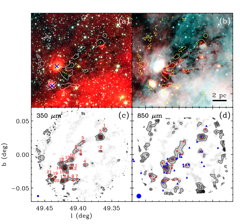
Figure 1.— Infrared and submillimeter maps of the IRDC G049.40–00.01. (a) IRAC three-color composite (8.0 µm in red, 4.5 µm in green, and 3.6 µm in blue) image overlaid with the 4$\sigma$ contour of the 350 µm map. Two large crosses mark the compact H II regions PR 29 and 30, from north to south (Phillips & Ramos-Larios, 2008). (b) IRAC and MIPS two-color composite (8.0 µm in cyan and 24 µm in red) image. The scale bar indicates 2 pc. (c) SHARC-II 350 µm image (both gray scale and contours). The compact sources (clumps) are labeled and marked by small crosses. Contour levels are 4, 8, 12, 16, and 20 $\times$ 0.09 (1$\sigma$) Jy beam^-1. (d) SHARC-II 850 µm image. Contour levels are 3, 6, 9, and 12 $\times$ 0.05 (1$\sigma$) Jy beam^-1. The crosses mark the positions of the 350 µm clumps. The filled triangles mark the YSOs from Kang et al. (2009). The FWHM resolutions of the SHARC-II maps are indicated in the bottom left corners. The extraneous contours (noisy areas) near the edges of the SHARC-II maps should be ignored.

2. OBSERVATIONS AND DATA

The observations were made on 2010 May 10 and 15 at the CSO 10.4 m telescope near the summit of Mauna Kea, Hawaii. We used the bolometer camera SHARC-II (Dowell et al., 2003). The instrument resolution of SHARC-II is 8$\farcs$0 at 350 µm and 19$\farcs$4 at 850 µm. The Dish Surface Optimization System was used to correct the dish surface for static imperfections and deformations due to gravitational forces as the dish moves in elevation (Leong et al., 2006). We obtained five scans at 350 µm for a total integration time of 50 minutes in moderate weather ($\tau_{225\rm GHz}\approx$ 0.046–0.068) and fourteen scans at 850 µm for a total integration time of 140 minutes in moderate weather ($\tau_{225\rm GHz}\approx$ 0.053–0.078). Pointing and calibration scans were taken on hourly basis on strong submillimeter sources: Neptune, Arp 220, IRAS 16293–2422, CRL 2688, W75N, and K 3-50. The data were reduced using version 2.01-2 of the software package CRUSH (Kovács, 2006, Comprehensive Reduction Utility for SHARC-II). The final maps were smoothed to angular resolutions of FWHM = 9$\farcs$61 at 350 µm and 23$\farcs$32 at 850 µm.

The Spitzer data presented here are the GLIMPSE and MIPSGAL data. The GLIMPSE and MIPSGAL are legacy programs covering the inner Galactic plane at 3.6, 4.5, 5.8, and 8.0 µm with the Infrared Array Camera (IRAC; Fazio et al., 2004) and at 24 and 70 µm with the Multiband Imaging Photometer for Spitzer (MIPS; Rieke et al., 2004), respectively.

3. RESULTS

Table 1Submillimeter Continuum Source Parameters

	Peak Position			Peak Flux		Total Flux	Size	24 µm	Associated
	$l$	$b$		850 $\micron$	350 $\micron$	at 350 $\micron$		Sources	YSOs
Source	(deg)	(deg)		(Jy beam-1)	(Jy beam-1)	(Jy)	($\arcsec\times\arcsec$)
1	49.361	0.037		0.30	0.58	3.4 $\pm$ 0.4	21 $\times$ 21	$\cdots$
2	49.366	0.005		0.24	0.54	1.6 $\pm$ 0.3	21 $\times$  8	2	345, 348
3	49.367	0.025		0.58	1.75	11.8 $\pm$ 1.1	22 $\times$ 19	2	346
4	49.390	–0.016		0.26	0.54	2.5 $\pm$ 0.2	26 $\times$ 21	3	362, 366, 367
5	49.393	0.019		0.23	0.55	5.1 $\pm$ 1.6	53 $\times$ 19	$\cdots$
6	49.396	–0.000		0.23	0.41	1.2 $\pm$ 0.1	16 $\times$ 15	1
7	49.401	–0.036		$\cdots$	0.54	1.6 $\pm$ 0.2	22 $\times$ 16	$\cdots$
8	49.403	0.005		0.27	0.56	4.4 $\pm$ 0.6	48 $\times$ 23	$\cdots$
9	49.408	–0.038		0.19	0.68	2.3 $\pm$ 0.3	29 $\times$ 13	1
10	49.409	–0.007		0.48	1.09	5.5 $\pm$ 1.1	21 $\times$ 18	3
11	49.410	–0.016		$\cdots$	0.63	1.4 $\pm$ 0.2	16 $\times$ 11	$\cdots$
12	49.412	–0.020		$\cdots$	0.99	2.2 $\pm$ 0.1	20 $\times$ 11	1
13	49.416	–0.010		$\cdots$	0.57	1.4 $\pm$ 0.3	21 $\times$ 11	1
14	49.418	–0.038		$\cdots$	0.88	3.4 $\pm$ 0.3	29 $\times$ 13	1
15	49.417	–0.027		$\cdots$	0.70	2.1 $\pm$ 0.5	14 $\times$ 13	$\cdots$
16	49.420	–0.021		0.65	1.96	13.3 $\pm$ 0.8	27 $\times$ 20	3	409, 414, 419
17	49.423	–0.040		0.41	1.44	5.6 $\pm$ 0.8	24 $\times$ 17	1	421
18	49.425	–0.013		0.27	1.02	4.3 $\pm$ 0.3	33 $\times$ 16	1
19	49.434	–0.034		0.21	0.72	1.2 $\pm$ 0.3	13 $\times$  7	$\cdots$
20	49.439	–0.038		0.26	1.31	3.4 $\pm$ 0.9	14 $\times$ 12	1
21	49.443	–0.032		0.40	0.94	2.3 $\pm$ 0.4	21 $\times$ 17	1	438

Figure 1 shows the maps of the Spitzer IRAC, MIPS, and SHARC-II 350 and 850 µm toward the IRDC G049.40–00.01. In the IRAC composite map (Figure 1a), a dark filamentary structure is seen in absorption against the background emission. The bright features in the IRAC composite map are two H II regions and bright diffuse emission from the active star-forming region W51 to the south. The spatial distribution of the dark filamentary structure agrees well with the distribution of the 350 µm emission. Figure 1b shows the two-color composite (IRAC 8.0 µm in cyan and MIPS 24 µm in red) image, overlaid with the 350 µm emission map. Some regions of G049.04–00.01 are still dark at 24 µm, implying low temperature and high column density. There are also many bright 24 µm point-like sources located within the IRDC. The dark features of the IRDC seen in the Spitzer maps appear in emission in the 350 and 850 µm maps (Figures 1c and 1d) because their cold thermal dust emission peaks at millimeter/submillimeter wavelengths. The bright clumps in the 350 µm map are well aligned with the 24 µm peaks, which suggests that the 24 µm sources are central stars of these dense clumps. The distribution of 850 µm emission is very similar to that of 350 µm emission except the details unresolved with the relatively large beam of the 850 µm map. The maximum flux densities are 1.96 $\pm$ 0.09 and 0.64 $\pm$ 0.05 Jy beam^-1 at 350 and 850 µm, respectively.

A total of 21 sources were identified as compact clumps for which peak flux densities are greater than the 4$\sigma$ level in the 350 µm continuum map by eye. When a peak is located close to another one, it is considered an independent peak if the peak intensity is higher than the intensity at the interface between them by 1$\sigma$ level or larger and if their separation is larger than a beam size. Table 1 lists the peak position, peak flux densities, 350 µm total flux density, size, number of associated 24 µm sources, and associated YSOs of each clump. The total flux density at 350 µm is measured from the emission in the circumscribed box of 2$\sigma$ contour. In crowded areas, the saddle point between adjacent clumps is used to limit the area for total flux measurements. The size represents the FWHM, deconvolved with the beam. In crowded areas, the intensity at the saddle point between adjacent clumps can be higher than the half-maximum intensity. In this case, we give the distance to the saddle point from the peak position as a size (in the direction to the adjacent clump). Column 8 lists the number of all 24 µm point sources detected with significant signal-to-noise ratios (S/N $>$ 4). Column 9 lists the YSOs in Kang et al. (2009). They used a detection criterion of S/N $>$ 7 at 24 µm to identify YSOs. The peak fluxes at 850 µm are measured only for the clumps having 850 µm peaks within the size boundaries of the 350 µm sources as described above. Table 2 lists the 850 $\micron$ total flux densities. For many clumps the 850 µm total flux cannot be measured individually because of crowding.

Table 2Total flux at 850 $\micron$

	Total Flux
Sources	(Jy)
1	0.30	$\pm$	0.05
2	0.29	$\pm$	0.13
3	1.03	$\pm$	0.15
4	0.26	$\pm$	0.05
5, 6, 8	0.98	$\pm$	0.18
7, 9	0.22	$\pm$	0.12
10, 13	0.79	$\pm$	0.15
11, 12, 15, 16, 18……	1.44	$\pm$	0.18
14, 17	0.73	$\pm$	0.15
19, 20, 21	0.51	$\pm$	0.14

Note. — For crowded areas, the total flux densities of each area are listed.

4. DISCUSSION

4.1. Physical Parameters

Continuum emission at 350 µm is sensitive to dust temperature, and the mass of molecular gas estimated from the 350 µm flux density depends on the assumed dust temperature that varies with the presence or absence of central heating by embedded protostars. The clumps without detectable 24 µm sources may be pre-protostellar (harboring no protostar). Hennemann et al. (2009) derived dust temperatures of 22 and 15 K for cores with and without 24 µm source, respectively. Stutz et al. (2010) found that the dust temperatures are $\sim$17.7 K near the protostar and $\sim$10.6 K for the starless core in the Bok globule CB 244. Pre-protostellar and protostellar cores in the IRDC G011.1–0.12 have core temperatures of 22 K (Henning et al., 2010). Wilcock et al. (2011) derived temperatures of 8–11 K at the center of the cores and 18–28 K at the surface using radiative transfer models of IRDC seen in Herschel observations. Peretto et al. (2010) reported that IRDCs are not isothermal, showing that the dust temperature decreases significantly within IRDCs, from background temperatures of 20–30 K to minimum temperatures of 8–15 K within the clouds. In this paper, we assume a dust temperature of 15 K for simplicity and for ease of comparison with Kauffmann & Pillai (2010) (see Section 4.3).

The masses of the submillimeter clumps in G049.40–00.01 were calculated using the 350 µm flux densities. The mass can be estimated by $M={F_{\nu}D^{2}}/{\kappa_{\nu}B_{\nu}(T_{d})}$, where $F_{\nu}$ is the flux density at 350 µm, $D$ is the distance to the source, $B_{\nu}$ is the Planck function, $T_{d}$ is the dust temperature, and $\kappa_{\nu}$ is the dust mass opacity. The value of $\kappa_{\nu}$ at 350 µm used to calculate the masses is $5.91$ cm² g^-1, from the coagulated dust model with thin ice mantles of Ossenkopf & Henning (1994). Table 3 lists the total mass within the 2$\sigma$ contour. The representative masses listed in Table 3 were calculated using a uniform temperature of 15 K. These masses can be underestimates for colder clumps (those without a 24 µm source) and overestimates for hotter clumps (those with 24 µm sources). Different assumptions on the dust temperature can increase or decrease the mass estimate by a factor of $\sim$3 (see the footnote of Table 3). The uncertainty of the mass caused by the uncertainty of the distance is $\sim$30%. The sum of the clump masses is $\sim$3,600 $M_{\odot}$.

Table 3Properties of the Clumps

	Mtotal			MFWHM			Concentration
Source	($M_{\odot}$)			($M_{\odot}$)
1	154	$\pm$	18	149	$\pm$	27	0.65 $\pm$ 0.18
2	73	$\pm$	14	54	$\pm$	20	0.73 $\pm$ 0.44
3	536	$\pm$	50	354	$\pm$	75	0.77 $\pm$ 0.05
4	113	$\pm$	9	127	$\pm$	14	0.65 $\pm$ 0.21
5	232	$\pm$	73	226	$\pm$	109	0.78 $\pm$ 0.54
6	54	$\pm$	5	58	$\pm$	7	0.57 $\pm$ 0.17
7	73	$\pm$	9	88	$\pm$	14	0.50 $\pm$ 0.08
8	200	$\pm$	27	217	$\pm$	41	0.55 $\pm$ 0.09
9	104	$\pm$	14	99	$\pm$	20	0.59 $\pm$ 0.08
10	250	$\pm$	50	182	$\pm$	75	0.72 $\pm$ 0.13
11	64	$\pm$	9	60	$\pm$	14	0.50 $\pm$ 0.07
12	100	$\pm$	5	103	$\pm$	7	0.64 $\pm$ 0.17
13	64	$\pm$	14	64	$\pm$	20	0.39 $\pm$ 0.06
14	154	$\pm$	14	171	$\pm$	20	0.69 $\pm$ 0.23
15	95	$\pm$	23	90	$\pm$	34	0.62 $\pm$ 0.13
16	604	$\pm$	36	455	$\pm$	54	0.67 $\pm$ 0.03
17	254	$\pm$	36	242	$\pm$	54	0.71 $\pm$ 0.14
18	195	$\pm$	14	231	$\pm$	20	0.54 $\pm$ 0.05
19	54	$\pm$	14	61	$\pm$	20	0.62 $\pm$ 0.08
20	154	$\pm$	41	139	$\pm$	61	0.64 $\pm$ 0.04
21	104	$\pm$	18	131	$\pm$	27	0.65 $\pm$ 0.08

Note. — The mass is based on the total flux density at 350 µm assuming $T_{d}$ = 15 K. If $T_{d}$ = 10 K, multiply by 4.1. If $T_{d}$ = 20 K, multiply by 0.47.

4.2. Comparison with Simple Models

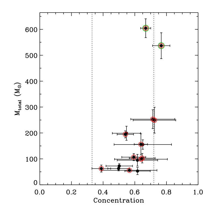
Figure 2.— Mass-concentration diagram for the clumps detected in the 350 µm map. Clumps with large ($>$ 0.2) uncertainties in concentration are omitted. Red and green circles represent clumps associated with 24 µm sources and green fuzzies, respectively (see Section 4.3). The vertical dotted lines ($C$ = 0.33 and 0.72) represent the limiting cases of stable Bonnor-Ebert spheres (Johnstone et al., 2000).

The clumps in G049.40–00.01 could be produced by gravitational fragmentation, and some simple quantities can be calculated to check the consistency. The average surface density is $\sim$0.04 g cm^-2 for the area within the 1$\sigma$ contour in the 350 µm map. With this surface density and the assumed dust temperature of 15 K, the critical wavelength of an isothermal, infinite, self-gravitating cylinder is $\lambda_{c}\approx 0.3$ pc, and the corresponding critical mass is $M_{c}\approx 5$ $M_{\odot}$ (Hartmann, 2002; Larson, 1985). For comparison, the projected distance between the nearest neighbours of clumps in G049.40–00.01 lies between 0.4 and 2 pc. The mean clump separation is 0.9 pc, and the average clump mass is 170 $M_{\odot}$. Many filamentary IRDCs fragment into clumps with a similar fragmentation scale (Henning et al., 2010; Miettinen & Harju, 2010). The difference between the calculated critical mass and the measured average mass probably indicates that the fragmentation history of G049.40–00.01 is more complicated than the fragmentation of an idealized simple cylinder. Previously suggested possibilities include an extra support by turbulence, changes of cloud temperature, and a compression by external forces (Onishi et al., 1998; Miettinen & Harju, 2010).

To study further physical conditions of the clumps, we compare the clumps to a static cloud model. The Bonnor-Ebert model describes the simplest self-gravitating pressure-confined isothermal sphere in a hydrostatic equilibrium (Ebert, 1955; Bonnor, 1956). The degree of self-gravitation within each clump can be estimated by calculating the degree of concentration of each clump. The concentration can be defined by $C=1-R_{\Sigma}$, where $R_{\Sigma}$ is the ratio of average to central column density (see equation (4) of Johnstone et al. (2000)). Small concentrations ($C<0.33$) imply uniform-density non-self-gravitating objects, and large values ($C>0.72$) imply critically self-gravitating objects (Johnstone et al., 2000). The concentrations of the submillimeter clumps are listed in Table 3. Figure 2 shows the concentration of the clumps against the clump mass. Most clumps in G049.40–00.01 have concentrations between 0.33 and 0.72. Clump 3 ($C=0.77\pm 0.05$) is more concentrated than what is permitted by stable Bonnor-Ebert spheres. In general, massive clumps seem to have high concentrations. It is interesting to note that the four highest-concentration clumps are also the highest-mass ones, and they are all associated with 24 µm sources, indicating ongoing star formation. Two of them also show signs of shocked gas (see Section 4.3). For the rest of the clumps, there is no clear difference between those with and without 24 µm sources.

4.3. High-mass Star Formation

Massive stars are expected to be formed in molecular clouds with a large mass concentrated in a relatively small volume. Kauffmann & Pillai (2010) suggested a threshold for massive star formation by comparing clouds with and without massive star formation: $m_{\rm KP}=870\ M_{\odot}\ r^{1.33}$, where $r$ is the effective radius (half of the geometric mean of the FWHM sizes in Table 1) in pc. Clouds/clumps more massive than this threshold seem to form massive stars. Parmentier et al. (2011) provided an explanation for the Kauffmann-Pillai threshold by calculating the probable mass of the most massive star formed in model clumps having power-law density profiles.

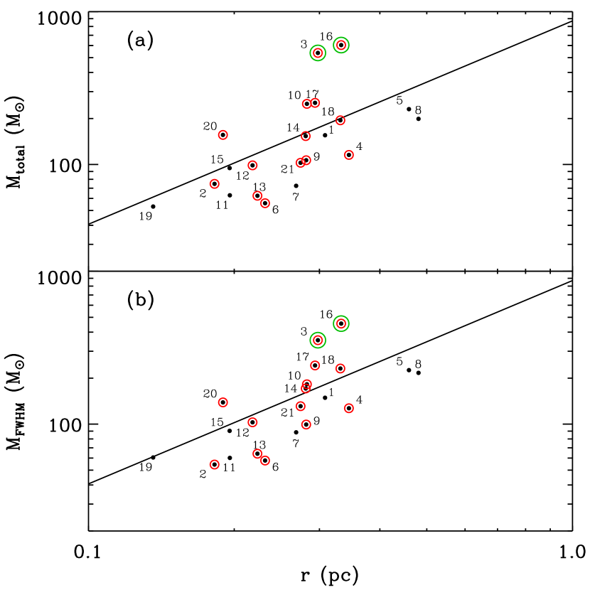
Figure 3.— Mass-size diagrams for the clumps detected in the 350 µm map. (a) Mass-size diagram with the total mass given in Table 3. (b) Mass-size diagram with the mass estimated from the flux density within the FWHM boundary (and with the dust opacity scaling factor applied, as suggested by Kauffmann & Pillai (2010)). Clumps associated with 24 µm sources are marked by red circles. Two large green circles mark the “green fuzzies”. The solid line represents the mass-size threshold for massive star formation, $m_{\rm KP}$, proposed by Kauffmann & Pillai (2010).

Figure 3 shows the mass-size relation for the clumps in G049.40–00.01. Kauffmann & Pillai (2010) assumed a dust temperature of 15 K. They used a dust opacity scaled by a factor of 1/1.5 (to match the masses estimated from dust emission and extinction) and a mass correction factor of 1/$\ln 2$ (to convert the total mass to the mass contained in the FWHM), and these factors cancel out almost exactly. Figure 3a shows the relation between the total mass and the effective radius. Figure 3b shows the relation between the mass contained within the FWHM boundary (with the opacity scaled by 1/1.5 to make a proper comparison with Kauffmann & Pillai (2010)) and the effective radius. The masses are listed in Table 3. All the clumps are distributed near $m_{\rm KP}$, within a factor of $\sim$3.5.

Association with bright 24 µm point-like sources is an indicator of star formation because 24 µm emission traces warm dust heated by the material accreting onto a central protostar. Fourteen clumps out of 21 have 24 µm point-like sources within their extent. The most massive ones (clumps 3 and 16) even show extended, enhanced 4.5 µm emission called “green fuzzies” or extended green objects, which indicate shocked gas (Chambers et al., 2009; Cyganowski et al., 2008). Extended 4.5 µm emission also indicates vigorous star-forming activity. In the G049.40–00.01 region, two compact H II regions (PR 29 and 30 in Figure 1a) were identified based on Spitzer data (Phillips & Ramos-Larios, 2008). PR 29 is more extended than PR 30 in the infrared maps (Figures 1a and 1b) and is not directly associated with a submillimeter clump. PR 29 seems to be a blister type H II region formed on the cloud surface near clump 18. In contrast, PR 30 is closely associated with the submillimeter clump 20, which suggests that it is still embedded in the dense cloud. PR 30 may be less evolved than PR 29. Clumps 3, 16, and 20 (clumps associated with “green fuzzies” or compact H II region) are located well above $m_{\rm KP}$, and this fact seems to corroborate the threshold for massive star formation suggested by Kauffmann & Pillai (2010).

Several clumps are dark at 24 µm, and they may be clumps either in the pre-protostellar phase or containing protostars of undetectably low luminosity. These clumps reside below $m_{\rm KP}$ in Figure 3 and may not be dense enough to form stars (yet). Therefore, objects in various stages of star formation (from pre-protostellar cores, protostars, to H II regions) are distributed in and around the IRDC G049.40–00.01.

Spectral observations would be required to definitively determine the evolutionary status of the clumps. Recent multi-wavelength, high angular resolution studies on IRDCs focused on the chemical, kinematic, and physical properties of the initial conditions for massive star formation. Pillai et al. (2011) investigated secondary massive cold cores in the vicinity of H II regions based on the line (NH₂D, NH₃, and HCO⁺) and millimeter continuum observations. They showed that the cores in the earliest stage of massive star formation are cold, dense, and highly deuterated ([NH₂D/NH₃] $>$ 6%). Devine et al. (2011) found an anti-correlation between NH₃ and CCS toward the IRDC G19.30+0.07 based on interferometric observations at 22 GHz. The different evolutionary states of the young objects in G049.40–00.01 can be investigated in detail by obtaining high-resolution interferometric data in the future.

5. SUMMARY

We observed the IRDC G049.04–00.01 in the 350 and 850 µm continuum with the SHARC-II bolometer camera. The dark features in the infrared images have a good agreement with the emission structure in the submillimeter images. Twenty-one clumps were identified based on the 350 µm continuum map, and the mass of each clump ranges from 50 to 600 $M_{\odot}$. The majority of these clumps are associated with bright 24 µm emission sources, indicating star-forming activity. The most massive clumps (clumps 3 and 16) show extended, enhanced emission in the IRAC 4.5 µm image. All the clumps are distributed near the threshold for massive star formation. The IRDC G049.04–00.01 contains objects in various evolutionary stages of star formation.

References

- Battersby et al. (2010) Battersby, C., Bally, J., Jackson, J. M., Ginsburg, A., Shirley, Y. L., Schlingman, W., & Glenn, J. 2010, ApJ, 721, 222
- Benjamin et al. (2003) Benjamin, R. A., et al. 2003, PASP, 115, 953
- Beuther et al. (2007) Beuther, H., Churchwell, E. B., McKee, C. F., & Tan, J. C. 2007, Protostars and Planets V, 165
- Beuther & Henning (2009) Beuther, H., & Henning, T. 2009, A&A, 503, 859
- Bonnor (1956) Bonnor, W. B. 1956, MNRAS, 116, 351
- Carey et al. (1998) Carey, S. J., Clark, F. O., Egan, M. P., Price, S. D., Shipman, R. F., & Kuchar, T. A. 1998, ApJ, 508, 721
- Carey et al. (2000) Carey, S. J., Feldman, P. A., Redman, R. O., Egan, M. P., MacLeod, J. M., & Price, S. D. 2000, ApJ, 543, L157
- Carey et al. (2009) Carey, S. J., et al. 2009, PASP, 121, 76
- Chambers et al. (2009) Chambers, E. T., Jackson, J. M., Rathborne, J. M., & Simon, R. 2009, ApJS, 181, 360
- Cyganowski et al. (2008) Cyganowski, C. J., et al. 2008, AJ, 136, 2391
- Devine et al. (2011) Devine, K. E., Chandler, C. J., Brogan, C., Churchwell, E., Indebetouw, R., Shirley, Y., & Borg, K. J. 2011, ApJ, 733, 44
- Dowell et al. (2003) Dowell, C. D., et al. 2003, Proc. SPIE, 4855, 73
- Ebert (1955) Ebert, R. 1955, ZAp, 37, 217
- Egan et al. (1998) Egan, M. P., Shipman, R. F., Price, S. D., Carey, S. J., Clark, F. O., & Cohen, M. 1998, ApJ, 494, L199
- Fazio et al. (2004) Fazio, G. G., et al. 2004, ApJS, 154, 10
- Hartmann (2002) Hartmann, L. 2002, ApJ, 578, 914
- Hennemann et al. (2009) Hennemann, M., Birkmann, S. M., Krause, O., Lemke, D., Pavlyuchenkov, Y., More, S., & Henning, T. 2009, ApJ, 693, 1379
- Henning et al. (2010) Henning, T., Linz, H., Krause, O., Ragan, S., Beuther, H., Launhardt, R., Nielbock, M., & Vasyunina, T. 2010, A&A, 518, L95
- Imai et al. (2002) Imai, H., Watanabe, T., Omodaka, T., Nishio, M., Kameya, O., Miyaji, T., & Nakajima, J. 2002, PASJ, 54, 741
- Johnstone et al. (2000) Johnstone, D., Wilson, C. D., Moriarty-Schieven, G., Joncas, G., Smith, G., Gregersen, E., & Fich, M. 2000, ApJ, 545, 327
- Kang et al. (2010) Kang, M., Bieging, J. H., Kulesa, C. A., Lee, Y., Choi, M., & Peters, W. L. 2010, ApJS, 190, 58
- Kang et al. (2009) Kang, M., Bieging, J. H., Povich, M. S., & Lee, Y. 2009, ApJ, 706, 83
- Kauffmann & Pillai (2010) Kauffmann, J., & Pillai, T. 2010, ApJ, 723, L7
- Kovács (2006) Kovács, A. 2006, Ph.D. Thesis, California Institute of Technology
- Lada & Lada (2003) Lada, C. J., & Lada, E. A. 2003, ARA&A, 41, 57
- Larson (1985) Larson, R. B. 1985, MNRAS, 214, 379
- Leong et al. (2006) Leong, M., Peng, R., Houde, M., Yoshida, H., Chamberlin, R., & Phillips, T. G. 2006, Proc. SPIE, 6275,
- Miettinen & Harju (2010) Miettinen, O., & Harju, J. 2010, A&A, 520, A102
- Onishi et al. (1998) Onishi, T., Mizuno, A., Kawamura, A., Ogawa, H., & Fukui, Y. 1998, ApJ, 502, 296
- Ossenkopf & Henning (1994) Ossenkopf, V., & Henning, T. 1994, A&A, 291, 943
- Parmentier et al. (2011) Parmentier, G., Kauffmann, J., Pillai, T., & Menten, K. M. 2011, MNRAS, 939
- Peretto & Fuller (2009) Peretto, N., & Fuller, G. A. 2009, A&A, 505, 405
- Peretto et al. (2010) Peretto, N., et al. 2010, A&A, 518, L98
- Phillips & Ramos-Larios (2008) Phillips, J. P., & Ramos-Larios, G. 2008, MNRAS, 391, 1527
- Pillai et al. (2011) Pillai, T., Kauffmann, J., Wyrowski, F., Hatchell, J., Gibb, A. G., & Thompson, M. A. 2011, arXiv:1105.0004
- Rathborne et al. (2005) Rathborne, J. M., Jackson, J. M., Chambers, E. T., Simon, R., Shipman, R., & Frieswijk, W. 2005, ApJ, 630, L181
- Rathborne et al. (2006) Rathborne, J. M., Jackson, J. M., & Simon, R. 2006, ApJ, 641, 389
- Rieke et al. (2004) Rieke, G. H., et al. 2004, ApJS, 154, 25
- Sato et al. (2010) Sato, M., Reid, M. J., Brunthaler, A., & Menten, K. M. 2010, ApJ, 720, 1055
- Simon et al. (2006a) Simon, R., Jackson, J. M., Rathborne, J. M., & Chambers, E. T. 2006a, ApJ, 639, 227
- Simon et al. (2006b) Simon, R., Rathborne, J. M., Shah, R. Y., Jackson, J. M., & Chambers, E. T. 2006b, ApJ, 653, 1325
- Stutz et al. (2010) Stutz, A., et al. 2010, A&A, 518, L87
- Wilcock et al. (2011) Wilcock, L. A., et al. 2011, A&A, 526, A159
- Xu et al. (2009) Xu, Y., Reid, M. J., Menten, K. M., Brunthaler, A., Zheng, X. W., & Moscadelli, L. 2009, ApJ, 693, 413