Tron, a combinatorial Game on abstract Graphs

Abstract

We study the combinatorial two-player game Tron. We answer the extremal question on general graphs and also consider smaller graph classes. Bodlaender and Kloks conjectured in [2] PSPACE-completeness. We proof this conjecture.

1 Introduction

The movie Tron from 1982 inspired the computer game Tron [4]. The game is played in a rectangle by two light cycles or motorbikes, which try to cut each other off, so that one, eventually has to hit a wall or a light ray. We consider a natural abstraction of the game, which we define as follows: Given an undirected graph $G$, two opponents play in turns. The first player (Alice) begins by picking a start-vertex of $G$ and the second player (Bob) proceeds by picking a different start-vertex for himself. Now Alice and Bob take turns, by moving to an adjacent vertex from their respective previous one in each step. While doing that it is forbidden to reuse a vertex, which was already traversed by either player. The game ends when both players cannot move anymore. The competitor who traversed more vertices wins. Tron can be pictured with two snakes, which eat up pieces of a tray of cake, with the restriction that each snake only eats adjacent pieces and starves if there is no adjacent piece left for her. We assume that both contestants have complete information at all times.

Bodlaender is the one who first introduced the game to the science community, and according to him Marinus Veldhorst proposed to study Tron. Bodlaender showed PSPACE-completeness for directed graphs with and without given start positions [1]. Later, Bodlaender and Kloks showed that there are fast algorithms for Tron on trees [2] and NP-hardness and co-NP-hardness for undirected graphs.

We have two kind of results. On the one hand we investigated by how much Alice or Bob can win at most. It turns out, that both players can gather all the vertices except a constant number in particular graphs. This results still holds for $k$-connected graphs. For planar graphs, we achieve a weaker, but similar result. We also investigated the computational complexity question. we showed PSPACE-completeness for Tron played on undirected graphs both when starting positions are given and when they are not given.

Many proofs require some tedious case analysis. We therefore believe that thinking about the cases before reading all the details will facilitate the process of understanding. To simplify matters, we neglected constants whenever possible.

2 Basic Observations

The aim of this section is to show some basic characteristics and introduce some notation, so that the reader has the opportunity to become familiar with the game.

Definition.

Let $G$ be a graph, and Alice and Bob play one game of Tron on $G$. Then we denote with $\#\texttt{A}$ the number of vertices Alice traversed and with $\#\texttt{B}$ the number of vertices Bob traversed on $G$. The outcome of the game is $\#\texttt{B}/\#\texttt{A}$. We say Bob wins iff $\#\texttt{B}>\#\texttt{A}$, Alice wins iff $\#\texttt{A}>\#\texttt{B}$ and otherwise we call the game a tie. We say Bob plays rationally, if his strategy maximizes the outcome and we say Alice plays rationally if her strategy minimizes the outcome. We further assume that Alice and Bob play always rational.

Here we differ slightly from [1], where Alice loses if both players receive the same amount of vertices. We introduce this technical nuance, because it makes more sense in regard of the extremal question and is not relevant for the complexity question.

Now when you play a few games of Tron on a ”random” graph, you will observe that you will usually end up in a tie or you will find that one of the players made a mistake during the game. So a natural first question to ask is if Alice or Bob can win by more than one at all.

Example 1 (two paths).

Let $G$ be a graph which consists of two paths of length $n$. On the one hand, Alice could start close to the middle of one of the paths, then Bob starts at the beginning of the other path, and thus wins. On the other hand if Alice tries to start closer to the end of a path Bob will cut her off by starting next to her on the longer side of her path. The optimal solution lies somewhere in between and a bit of arithmetic reveals that for the optimal choice $\#\texttt{B}/\#\texttt{A}$ tends to $2/(\sqrt{5}-1)$ as $n$ tends to infinity.

And what about Alice? We will modify our graph above by adding a super-vertex $v$ adjacent to every vertex of $G$. Now when Alice starts there the first vertex on $G$ will be taken by Bob and Alice will take the second vertex on $G$. So we see that the roles of Alice and Bob have interchanged.

Lemma 1 (Super-vertex).

Let $G$ be a graph where $\left(\#\texttt{B}\right/\#\texttt{A})_{G}>1$ and $F$ be the graph we obtain by adding a super-vertex $v$ adjacent to every vertex of $G$. It follows that

$$\left(\frac{\#\texttt{A}}{\#\texttt{B}}\right)_{F}\geq\left(\frac{\#\texttt{B}}{\#\texttt{A}}\right)_{G}.$$

So lemma 1 simplifies matters. Once we have found a good graph for Bob we have automatically found a good graph for Alice. But the other direction holds as well. Let $G$ be a graph where Alice wins and let us say she starts at vertex $v$. Delete vertex $v$ from $G$ to attain $H$. Now the situation in Alice’s first move in $H$ is the same as Bob’s first move in $G$. And Bob’s first move in $H$ includes the options Alice had in her second move in $G$.

Lemma 2.

Let $G$ be a graph where $\left(\#\texttt{B}\right/\#\texttt{A})_{G}<1$ and $H$ be the graph we obtain by deleting the vertex where Alice starts. It follows that

$$\left(\frac{\#\texttt{B}+1}{\#\texttt{A}}\right)_{H}\geq\left(\frac{\#\texttt{A}}{\#\texttt{B}}\right)_{G}.$$

Note that the starting vertex of Alice need not be unique, even when Alice wins. To see this consider the complete graph with an odd number of vertices.

Bodlaender and Kloks [2] showed the first equation of lemma 3 in theorem 3.1.

Lemma 3 (Trees).

Let $T$ be a tree then $\#\texttt{A}\leq\#\texttt{B}+1$ and $\#\texttt{B}\leq 2\cdot\#\texttt{A}$

Proof.

The idea of the proof is to describe a strategy for Alice and Bob explicitly. Let $v$ denote the starting vertex of Alice with $w_{1},\ldots,w_{k}$ its neighbors and $l_{i}$ the length of the longest path from $w_{i}$ in $T-\{v\}$ for all $i=1,\ldots,k$. Further, we denote with $j$ an index which satisfies $l_{j}=\max_{i=1,\ldots,k}{l_{i}}$. If Bob chooses $w_{j}$ as start-vertex and thus obtains at least $l_{j}$, while Alice receives at most $l_{j}+1$.

For the second inequality, let Alice start in the middle of a longest path. Thus she divides the tree into smaller trees $T_{1},\ldots,T_{k}$. Bob chooses one of them and receives at most as many vertices as the length of longest path in $T$. Alice will enter a different tree, which contains one half of the longest path. So she receives at least half of the longest path. ∎

3 Extremal Question

In this section we want to answer the extremal question for Tron. That is: Is there a non-trivial upper bound on $\#\texttt{B}/\#\texttt{A}$ as a function of the number of vertices of $G$? The answer is surprisingly no. For every natural number $n$ exists a graph with $n$ vertices, such that $\#\texttt{B}=n-c$ for some constant $c$. The idea behind it is fairly easy. Think of two motorcycles on a highway. If one of the motorcycles pushes the other from the highway to the smaller and slower country roads, it can encircle the other using the highway and traverse the rest of the map comfortably alone.

It seems convenient to study a simpler example first.

Example 2 (big-circle).

In this example we consider a cycle of length $n$, and a subtle change of the rules. We assume, that Alice has to make two moves before Bob joins the game. Now the analysis of this example is short: Alice decides for a vertex and a direction and Bob can simply start in front of her and take the rest of the circle. This example will also work, if only every $100^{th}$ vertex is an admissible start-vertex for Bob.

Example 3 (visage).

This example consists of three parts: an overhead graph, a big-circle and a bottleneck as depicted on the left-hand side of figure 1. The overhead graph can be any graph where Bob wins. The two paths in example 1 give us such a graph. It suffices to take paths of length $3$ for our purpose. The big-circle consists of a large cycle of length $4*l$. The last part is a bottleneck between the first two parts and consists of two singular vertices. The bottleneck is adjacent to every vertex of the overhead graph but only to every fourth vertex of the cycle. Alternating between the two bottleneck vertices.

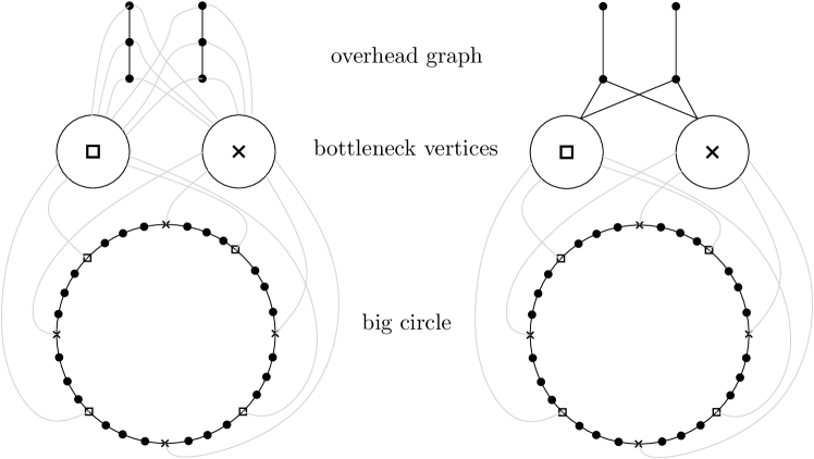
Figure 1: The ordinary visage on the left-hand side and the visage from Torsten Ueckerdt on the right-hand side.

Bob has a strategy to gather $n-c$ vertices, where $n$ denotes the total number of vertices in the visage and $c$ some constant.

Proof.

We will give a strategy for Bob for all possible moves of Alice.

Case1 Alice starts in the overhead graph. Bob will then also start in the overhead graph and win within the overhead graph. So Alice has to leave the overhead graph eventually and go to one of the bottleneck-vertices. Bob waits one more turn within the overhead graph. If Alice tries to go back to the overhead graph, Bob will go to the other bottleneck-vertex and trap her. Thus Alice will have to go to the big-circle and once there she will have made already two turns when Bob enters the big-circle. We already studied this situation in example 2.

Case2 Alice starts in one of the bottleneck vertices. Bob will then again start somewhere in the overhead graph. The situation is as in case 1.

Case3 At last we consider the case where Alice starts in the big-circle. In this case, Bob will start on the closest bottleneck-vertex to Alice and then quickly go to the other bottleneck-vertex via the overhead graph. Thus she cannot leave the big-circle. Finally he enters the big-circle and cuts her off. ∎

Example 4 (Torsten-visage).

Torsten Ueckerdt showed with a very similar construction how to reduce $c$ to $8$. As depicted on the right hand side of figure 1. Here not every vertex of the overhead graph is connected to the bottleneck. We want to point out, that the crossing number is two, so the graph is almost planar. We omit the proof as it does not involve any new ideas.

In addition, lemma 1 gives us a graph where Alice can obtain all vertices except a constant amount. The natural question is, for which graph classes is this kind of construction possible. Which graph classes should we consider?

Very interesting is always the planar case, because planar graphs are very well studied and very close to the original game. We will show that we have graphs with $\#\texttt{B}/\#\texttt{A}=\Theta(\sqrt{n})$ and graphs with $\#\texttt{A}/\#\texttt{B}=\Theta(\sqrt{n})$.

In the visage, Aliceś first move on the big-circle gives her a direction and she cannot reconsider. This was the key for Bob to be able to cut her off. In a highly connected graph, we expect intuitively that Alice has enough freedom to avoid to get imprisoned. This motivates us to study $k$-connected graphs. Surprisingly, we are able to adapt the visage so that it becomes arbitrarily highly connected.

3.1 Planar Graphs

We construct a planar visage. Again it will be more convenient to study a simpler example first.

Example 5 (long-path).

We consider now a path of length $n$, again with the subtle change of rules, that Alice has to make two moves before Bob starts. Now let us say, that Alice goes along the path and has $x$ vertices she might be able to reach. Well, if Bob cuts her off the outcome will be $\#\texttt{B}/\#\texttt{A}=\Theta(x)$. So Alice could choose $x$ to be fairly small. But then Bob would just choose the other side and the outcome would become $\#\texttt{B}/\#\texttt{A}=\Theta(n/x)$. This observation implies that Alice best choice is to choose $x=\Theta(\sqrt{n})$ and thus the value of the game is $\Theta(\sqrt{n})$.

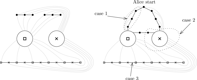
Figure 2: planar visage for Bob

The reader might already guess the planar visage we present now.

Example 6 (planar visage).

The planar visage differs from the visage, only in one point, namely the big-circle is replaced by a long path. We can see from the drawing on the left-hand side of figure 2, that this graph is planar. It is clear that the value is $\Theta(\sqrt{n})$

Unfortunately we cannot apply lemma 1 to obtain a planar graph where Alice wins. Even if we add a super-vertex which is only connected, to wisely chosen vertices. Instead we construct a new overhead graph.

Example 7 (planar visage for Alice).

This example is different from the previous one in two ways. Obviously the overhead graph has changed, as you can see on the left had side of figure 2, but more subtly the distance between vertices adjacent to the bottleneck increased from $4$ to $7$. We claim that $\#\texttt{A}/\#\texttt{B}=\Theta(\sqrt{n})$

Proof.

We give an explicit strategy for Alice. Alice’s start-vertex is marked in figure 2.

Case 1 Bob starts somewhere on a path from Alice’s start-vertex to a bottleneck-vertex. Alice can just go directly to the corresponding bottleneck-vertex and trap Bob this way.

Case 2 Bob starts w.l.o.g. on the $\times$-vertex or on the adjacent vertex on the path between the two bottleneck vertices. Alice will slowly go to the $\Box$-vertex, but hurry up, if Bob shows any sign that he wants to go in that direction as well.

Case 3 The only remainung case is where Bob starts on the long path. Alice will go to the bottleneck-vertex, which is closer to Bob and then to the other bottleneck-vertex. Thus Bob cannot leave the long path and Alice enters it second. ∎

We end the section on planar graphs with a remark, that in both planar visages we presented, it is possible for the winning player to cut off his or her opponent within at most 20 turns. But this might not be the optimal strategy, as shown in example 5. Thus you cannot proof a lower bound of $\Omega(\sqrt{n})$, by showing that each player receives at least $\Omega(\sqrt{n})$ vertices. However, the author feels that a totally different kind of idea would be needed to improve the planar visage. We conjecture that the upper bound is tight.

3.2 $k$-connected Visage

Now we show how to construct a $k$-connected visage. The essence is twofold. First, we increase the number of bottleneck-vertices and secondly we replace paths of the big-circle by double-trees which will be introduced shortly. Double-trees have a high-connectivity, a bottleneck and the vertex-set can be traversed entirely.

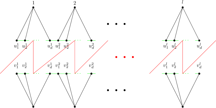
Figure 3: All the leaves with their names and parents. In green is the edge-set $E_{1}$ indicated and in red one of the cycle partitioning the set of leaves.

Example 8 (Double-tree).

A double-tree of degree $d$ and height $h$ consists of two fully balanced rooted trees with $d$ children for each inner vertex and height $h$. The two double-trees are connected as explained below.

From left to right we name the leaves of the upper half of the double-tree

$$u_{1}^{1},u_{2}^{1},u_{3}^{1},\ldots,u_{d}^{1},u_{1}^{2},u_{2}^{2},u_{3}^{2},\ldots,u_{d}^{2},\ \ldots\ ,u_{1}^{l},u_{2}^{l},u_{3}^{l},\ldots,u_{d}^{l}$$

and likewise we name the leaves from the lower half of the double-tree

$$v_{1}^{1},v_{2}^{1},v_{3}^{1},\ldots,v_{d}^{1},v_{1}^{2},v_{2}^{2},v_{3}^{2},\ldots,v_{d}^{2},\ldots,v_{1}^{l},v_{2}^{l},v_{3}^{l},\ldots,v_{d}^{l}$$

as depicted in figure 3. With $l$ we denote the number of parents of the leaves.

We add edge-set

$$E_{1}=\left\{(u_{i}^{j},u_{i+1}^{j}):i=1,\ldots,(d-1),j=1,\ldots,l\right\}$$

$$\cup\left\{(u_{d}^{j},u_{1}^{j+1}):j=1,\ldots,(l-1)\right\}$$

$$\left\{(v_{i}^{j},v_{i+1}^{j}):i=1,\ldots,(d-1),j=1,\ldots,l\right\}$$

$$\cup\left\{(v_{d}^{j},v_{1}^{j+1}):j=1,\ldots,(l-1)\right\}$$

and

$$E_{2}=\left\{(u_{n}^{j},v_{m}^{j}):j=1,\ldots,l;n\leq m\right\}$$

$$\cup\left\{(u_{n}^{j},v_{m}^{j+1}):j=1,\ldots,(j-1);m<n\right\}\\$$

$$\cup\left\{(u_{n}^{l},v_{m}^{1}):m<n\right\}.$$

Figure 4: The induction step of lemma 4

Lemma 4.

Let $T_{1},T_{2},\ldots,T_{n}$ be some trees. And each inner-vertex has at least $2$ children. Now we draw all the trees crossing-free in a half plane s.t. all leaves are on the boundary of the half plane. We define leaves as adjacent iff the line segment connecting them does not contain any other vertex. It follows, that there is an Hamilton-path from the leftmost to the rightmost leaf.

Proof.

We construct a special partition of the vertex-set of the trees into paths starting and ending in adjacent leaves. In a second step we just connect these paths canonically.

We do the first step by induction. If every tree is just a single vertex we define the partition to be the collection of all one element sets. Now let $T_{1},T_{2},\ldots,T_{n}$ be some trees as described above and $r$ a root of $T_{i}$ and we assume, that $T_{i}$ consists of more than one vertex. Let $v_{l}$ be the rightmost leaf of the leftmost subtree of $T_{i}$ and $v_{r}$ the leftmost leaf of the second subtree (left to right) of $T_{i}$. See figure 4. There exists exactly one path from $v_{l}$ to $v_{r}$ via $r$ within $T_{i}$. We add this path to the partition set and delete it from the trees. Thus we end up with a new bunch of trees with fewer vertices in total which we can partition by induction.

Now we connect the right end of each path to the left end of the next path to get the desired Hamilton-path. ∎

Lemma 5.

There is an Hamilton-path from one root of the double-tree to the other root.

Proof.

We start our tour at the top root and go down to $u_{1}^{1}$ and from there to $u_{2}^{1}$. Next we use the path constructed in lemma 4 to traverse the rest of this half of the double-tree. After ferrying over from $u_{d}^{l}$ to $v_{d}^{l}$ we copy our path in reverse order and thus have traversed every vertex without reusing any. ∎

Lemma 6.

The double-tree is d-connected

Proof.

For any $2$ nodes we will show that there are $d$ vertex-disjoint paths connecting them. And thus by Menger’s theorem [3, section 3.3], we know that the graph is $d$-connected. Close Observation shows that there are $d$ vertex-disjoint cycles partitioning the leaves. Cycle $i$ is described via $u^{1}_{i},v^{1}_{i},u^{2}_{i},v^{2}_{i},u^{3}_{i},v^{3}_{i},\ldots,u^{d}_{i},v^{d}_{i}$, see the red path in figure 3. To find $d$ vertex-disjoint paths from some $w_{1}$ to some $w_{2}$, it suffices to show that there exist $d$ vertex disjoint paths to the $d$ different cycles. This is clear for every leaf. It is also clear for every inner vertex as every inner vertex has $d$ children and every parent of a leaf is adjacent to all $d$ cycles. To construct $d$ disjoint paths from $w_{1}$ to $w_{2}$, we use $d$ vertex-disjoint direct paths from $w_{1}$ to the cycles and from $w_{2}$ to the cycles. These paths can be connected to each other, via the cycles. The only thing that can go wrong, is that a path from w.l.o.g. $w_{1}$ to a cycle uses $w_{2}$. But this can only happen once and would give us a path from $w_{1}$ to $w_{2}$, which is disjoint from the others. ∎

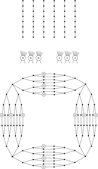
Figure 5: A $3$-connected visage with $4$ double-trees, the leaves marked with a $\Square$ are connected with a $\Square$-bottleneck-vertex and likewise leaves marked with a $\times$ are connected with a $\times$-bottleneck-vertex. For clarity of the drawing we we chose the height of the double-trees too small and omitted some edges of the double-trees.

Lemma 7 (Many afar leaves).

For all natural numbers $m,n$ and $d\geq 2$ there exists some $h_{0}\in\mathbb{N}$ such that a double-tree with height $h\geq h_{0}$ and degree $d$ has at least $m$ leaves which all have pairwise distance at least $n$.

Proof.

Every vertex has at most degree $c=d+3$. The number of leaves grows strictly monotone with $h$. In fact, it grows exponentially.

We proceed by induction on $n$. If we have leaf $v$, then we have at most $c+c^{2}+c^{3}+\ldots+c^{m}$ many leaves within distance $m$ to $v$ and thus we can find a leaf $w$ which has distance larger than $m$ to $v$, if we choose $h_{0}$ large enough. This shows the base case $n=2$.

On the other hand $n$ leaves have at most $n(c+c^{2}+c^{3}+\ldots+c^{m})$ leaves within distance $m$ and thus we could find a leaf which has distance $m$ to all the other leaves, if $h_{0}$ is large enough. This proves the induction step. ∎

Example 9 ($k$-connected visage).

The $k$-connected visage is depicted in figure 5. It consists again of three parts: The overhead graph is composed out of $k$ sufficiently long paths. The bottleneck-vertices are separated into two groups each of $k$ $\Square$-vertices and $k$ $\times$-vertices. Every vertex of the overhead graph is connected to every vertex of the bottleneck. The big-circle consists of degree $k$ double trees which we string together by their roots like a jeweler strings pearls together in a necklace. Now the height $h$ of the double trees is picked such that each double tree has $k$ leaves, which all have pairwise distance at least $2k$, see lemma 7. On these spots we connect alternating either $k$ $\Box$-vertices or $k$ $\times$-vertices. This construction is indeed $k$-connected and #B is everything but a constant.

Proof.

To see $k$-connectedness we assume $(k-1)$ vertices have been deleted. We will show that the graph is still connected. It suffice to show that, we can still connect every vertex to one of the bottleneck-vertices, let us say $v$. This is clear for any vertex of the overhead graph. Any other vertex of the bottleneck is connected to $v$ via any vertex of the overhead graph. In lemma 6 we showed, that every double-tree is $k$-connected. Thus every vertex stil has a path to a leaf that is connected to one of the bottleneck-vertices, which is itself connected to $v$.

To prove that #B is everything but a constant, we only point out where Bobs strategy differs from his strategy for the ordinary visage.

• Bob can wait arbitrarily long in the overhead graph, before he has to enter the big-circle if the paths are long enough, but still constant length as a function of $n$.

• Alice might go back and forth between the overhead graph and the bottleneck. While she does that, Bob can maintain that the number of $\Box$-vertices equals the number of $\times$-vertices. Thus when Alice enters the big-circle via one kind of vertex, Bob can still enter via the other kind, at some much later stage.

• Once Alice enters the big-circle (w.l.o.g. via a $\Square$-vertex.) Bob can traverse all remaining $\Square$-vertices in $2k-3$ moves and thus prevent Alice from returning to the overhead graph.

• After a constant number of turns in the big-circle Alice has to use a root of a double tree. This forces her to decide for a direction, she wants to go on the big-circle. Accordingly Bob enters the big-circle, once she has decided and cuts her off by reaching the next root on the big-circle earlier than she does.

∎

Adding a super-vertex as in lemma 1 gives us instantly a $k$-connected visage which is good for Alice.

4 Complexity Question

In this section we show that Tron is PSPACE-complete. To do this, it turned out to be convenient to consider variations where the graph is directed and/or start positions for Alice and Bob  are given. We reduce Tron to quantified boolean formula(QBF). It is well known, that it is PSPACE-complete to decide if a QBF $\varphi$ is true. A quantified boolean formula has the form $\varphi\equiv\exists x_{1}\forall x_{2}\exists x_{3}\forall x_{4}\ldots:C_{1}\wedge\ldots\wedge C_{k}$ with each $C_{i}\equiv L_{i_{1}}\vee L_{i_{2}}\vee L_{i_{3}}$ and $L_{i_{j}}$ some Literals) [5, section 8.3]. In theorem 1 we will construct for each $\varphi$ a directed graph $G_{\varphi}$ with given start positions $v_{1}$ and $v_{2}$ such that Alice has a winning strategy if and only if $\varphi$ is true. In theorem 2 we will modify this graph, such that it becomes undirected. In theorem 3 we will construct a directed overhead graph to $G_{\varphi}$, which will force Alice and Bob to choose certain starting positions. At last in theorem 4 we will construct an undirected overhead graph. Here we will make use of the constructions of the preceding theorems.

Figure 6: $G_{\varphi}$

Theorem 1 has already been proven by Bodlaender [1] and is similar to the proof that generalized geography is PSPACE-complete [5]. We repeat his proof, with subtle changes. These differences are necessary for theorem 2, 3 and 4 to work.

Theorem 1.

The problem to decide if Alice has a winning strategy in a directed graph with given start positions is PSPACE-complete.

Proof.

Given a QBF $\varphi$ with $n$ variables and $k$ clauses we construct a directed graph $G_{\varphi}$ as depicted in figure 6. It consists of starting positions for Alice and for Bob from where variable-gadgets begin such that Alice and Bob have to decide whether they move left or right which represents an assignment of the corresponding variable. Thereafter Alice has to enter a path of length $k-1$, which we call the waiting queue. Meanwhile Bob can enter the clause gadget, which consists of $k$ vertices arranged in a directed cycle each representing exactly one clause. Thus Bob can traverse all but one clause-vertex before Alice enters the clause-gadget. When she enters, she has only one clause-vertex to go to, which was chosen by Bob. Now from each clause-vertex we have edges to the corresponding variables and one edge to a dummy-vertex. So each player can make at most one more turn. Thus Bob takes the dummy-vertex. Consequently if $\varphi$ was true Alice had a strategy to assign the variables in a way that every clause becomes true and she is still able to make one more turn and therefore wins. Otherwise Bob has a strategy to assign the variables, such that at least one clause is false. Thus Alice cannot move anymore from the clause-vertex and the game ends in a tie. This shows PSPACE-hardness. As the game ends after a linear number of turns, it is possible to traverse the game tree using linear space. See [5] for a similar argument. ∎

Our approach is to take the graph $G_{\varphi}$ from theorem 1 and convert it to a working construction for theorem 2.

Theorem 2.

The problem to decide whether Alice has a winning strategy in an undirected graph with given start positions is PSPACE-complete.

Proof.

We replace every directed edge of $G_{\varphi}$ by an undirected one. Further, we will carry out $4$ modifications and later prove, that the resulting graph $G_{\varphi}^{\prime}$ has the desired properties.

Modification 1 (slow-path).

As we want that Alice and Bob assign each variable in order, we must prevent them from using the edge from a variable-vertex to a clause-vertex. We achieve this via elongating every such edge to a path of length $2k+n$. See figure 7.

(a) Modification of the waiting queue

(b) The way from a clause-vertex to a variable-vertex

Figure 7: Two of the modifications

Modification 2 (waiting queue).

The next motion that might happen, is that Bob cuts off the waiting queue. We prevent this by replacing the waiting queue by the graph depicted in figure 7.

Modification 3 (dummy-vertex).

Another concern is that Bob might go towards the dummy-vertex and return. To hinder this we replace all the edges to the dummy-vertex by the construction in figure 8.

Figure 8: Modification of the paths to the dummy-vertex

Modification 4 (spare-path).

It might be advantegous for Bob to go to a literal, which is contained in two clauses, instead of going to the dummy-vertex, because he then might use the return-path to a clause-gadget and receive in total $4k+2n+1$ vertices after leaving the clause-gadget. We attach a path of length $2n+k$ to each variable-vertex and the dummy-vertex.

We show first, that after Alice and Bob leave their respective start positions, they have to assign the variables. There are only two strategies they possibly could follow instead. The first is to use a spare-path from modification $4$. This gives at most $2n+k$ many vertices. The other player would just go down to the dummy-vertex and proceed to the spare-path from the dummy-vertex. Thus using the spare-path at this stage leads to a loss. The other option is to use a slow-path from a variable to the clause-gadget as introduced in modification $1$. It takes quite a while to traverse this path and meanwhile, the other player can just go down to the clause-gadget, traverse all the clause-vertices and then go to the dummy-vertex. Again, it turns out that this strategy is not a good option.

So we have established that Bob reaches the clause-gadget, Alice reaches the waiting queue and they have assigned all the variables alternatingly on their way. Now Bob could make one of two plans we would not like. The first plan is that he might try to go to the dummy-vertex and return before Alice has reached a clause-vertex. But the time to return is so long that Alice will have taken all the clause-vertices meanwhile and Bob would receive more vertices if he were to proceed all the way to the dummy-vertex and take the spare-path.

The second plan he might pursue is to short-cut the waiting queue. Luckily, the queue splits after $2$ vertices. So when Bob enters the queue before $2$ turns, Alice can avoid him by taking a different branch and the planner himself gets trapped. If he waits $2$ turns, he must have determined a clause-vertex for Alice already. So Alice knows which branch to use. This particular branch cannot be reached by Bob by then. So our constructions have circumvented his plans again.

In summary we have established that Bob  indeed has to traverse $k-1$ clause-vertices and Alice obviously has to go to the clause-vertex Bob left for her. What now? It is Bobs turn. One of the longest paths that remains goes to the dummy-vertex and proceeds via a spare-path. So he had better take it, because otherwise Alice will take it and he loses.

Now it is Alice turn. If there is a variable-vertex she can reach, she also has a path of the same length as Bob does and this would imply that she will win. If not, then she could only go towards a variable-vertex and Bob will win.

And again as in theorem 1 Alice has a winning strategy in $G^{\prime}_{\varphi}$ if and only if $\varphi$ is satisfiable. ∎

Now we show how to force Alice and Bob to choose certain start positions in a directed graph. We will do that by constructing a graph $H(G)$, such that Alice wins in $H(G)$ if and only if Alice wins in $G$ when both players start at certain positions $v_{1}$ and $v_{2}$. It follows, that Alice wins in $H(G_{\varphi})$ if and only if $\varphi$ is true. With a similar but different construction, theorem 3 was shown in [1]. Here we give a slightly different proof again, because it is an essential step for our proof of theorem 4.

Theorem 3.

The problem to decide whether Alice has a winning strategy in a directed graph without given start positions is PSPACE-complete.

Proof.

Assume we are given some directed graph $G$ and two vertices $v_{1},v_{2}\in G$. We construct some directed Graph $H(G)$ such that Alice wins in $H(G)$ if and only if Alice wins in $G$ with the predefined start-positions $v_{1},v_{2}$. Applied to $G_{\varphi}$, this finishes the proof.

The general idea of such an overhead graph is simple. We construct two vertices, which are very powerful, so Alice and Bob want to start there, but once there, they are forced to go to the start-vertices of the original graph. The idea is also used in theorem 4.

We describe the construction of $H(G)$ as depicted in figure 9 in detail:

We add two vertices $u_{1}$ and $u_{2}$ with attached directed paths of length $2n=2\#V(G)$ to the start-vertices $v_{1}$ and $v_{2}$ respectively. Now the longest path starts at $u_{1}$ or $u_{2}$ and has length between $2n$ and $3n$. Let $l_{low}=2n$ denote a lower bound on the length $l$ of the longest path in $G$ and $l_{up}=3n$ an upper bound on $l$.

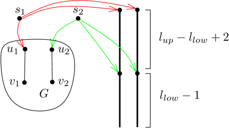
Figure 9: H(G)

Then we add two directed auxiliary-paths of length $l_{up}+1$ and vertices $s_{1}$ and $s_{2}$. The vertex $s_{1}$ is attached to $u_{1}$ and the two upper parts of the auxiliary-paths. The vertex $s_{2}$ is connected to $u_{2}$ and the middle parts of auxiliary-paths, such that the larger part is below, but the larger part is still shorter than the longest path from $u_{1}$ or $u_{2}$. This is possible as long as $l_{up}-l_{low}+2<l_{low}-1$, which is the case. We want to point out that once one of the players is in an auxiliary-path or $G$, there is no way out of the respective component simply because there is no outgoing edge.

Assume Alice starts at $s_{1}$ and Bob at $s_{2}$. Then Alice should go to $u_{1}$ because otherwise Bob will go into the same auxiliary-path as her and receive more vertices than Alice and thus she loses. Meanwhile, Bob should go to $u_{2}$ on his first turn, as he would receive fewer vertices in an auxiliary-path than Alice in $G$. Now we show, that it is best for Alice to start at $s_{1}$.

Case 1 Alice starts in $G$ Then Bob just starts at the top of an auxiliary-path.

Case 2 Alice starts in an auxiliary-path. As the path is directed, Bob starts in front of her.

Case 3 Alice starts in $s_{2}$. Then Bob starts in $s_{1}$. Now Bob can get $l_{up}+2$ in total and Alice at most $l_{up}+1$.

Thus Alice is better off starting at $s_{1}$, or she will lose anyway. We show now that under these conditions, Bob is always better off starting at $s_{2}$.

Case 4 Bob starts in an auxiliary-path. Alice will go to the other auxiliary-path and win.

Case 5 Bob starts in $G$. Alice will then just go to an auxiliary-path. ∎

Now the last task is to show the result if the graph is undirected and the starting positions are not given. We will do that by using the graph $G_{\varphi}^{\prime}$ and an undirected version of $H(G)$ which we will denote by $H^{\prime}(G)$. Unfortunately this will not work immediately. We will therefore construct an overhead graph $F(H^{\prime}(G))$ using some properties of $H^{\prime}(G)$.

Theorem 4.

The problem to decide whether Alice has a winning strategy in a undirected graph without given start positions is PSPACE-complete.

Proof.

The general idea of this construction is the same as in the previous proof, but because we build up from the construction from theorem 3, everything gets more involved. Every single argument is still elementary.

Let $H^{\prime}(G)$ be the graph $H(G)$ with all directed edges replaced by undirected ones. Also the auxiliary paths have to be changed slightly, because $l_{low}=4n$ and $l_{up}=5n$. We observe $5$ properties of this $H^{\prime}(G)$:

1. If Alice starts at $s_{1}$ and Bob starts at $s_{2}$, then Alice has to go to $u_{1}$ and Bob to $u_{2}$.

2. If Alice starts at $s_{2}$ and Bob at $s_{1}$, Bob will win.

3. If we assume $s_{1}$ and $s_{2}$ are forbidden to use, except when started at, it holds that the longest path starts at $s_{1}$. (longest path in the sense that we consider only one player.)

4. Any path from $s_{1}$ to $s_{2}$ can be extended using an auxiliary-path.

5. The shortest path from $s_{1}$ to $s_{2}$ has length at least $3$.

Properties p1 and p2 hold for directed graphs according to the proof of theorem 3, and hold by the same arguments for the undirected case. Property p3 is clear by the definition of the auxiliary paths. p4 is clear because any path from $s_{1}$ to $s_{2}$ uses at most one auxiliary path. Thus the path can be extended to an auxiliary path that has not been used yet. To p5 we remark that we consider only sufficiently large $n$.

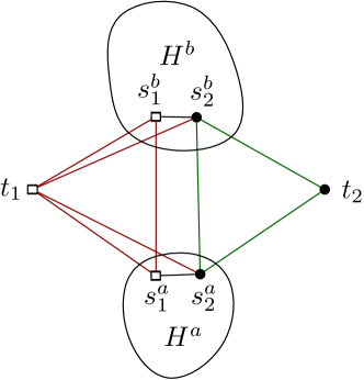
Figure 10: $F(H^{\prime}(G))$

We construct an overhead graph of $H^{\prime}(G)$, namely $F(H^{\prime}(G))$, as depicted in figure 10. It consists of two copies of $H^{\prime}(G)$, which we call $H^{a}$ and $H^{b}$. In addition two vertices $t_{1}$ and $t_{2}$. We indicate with an upper index ^a or ^b whether a vertex belongs to $H^{a}$ or $H^{b}$. We will always go w.l.o.g. to $H^{a}$ instead of $H^{b}$ when the situation is symmetric. The edge-set consists of all the edges in $H^{a}$, $H^{b}$ and $(t_{1},s^{a}_{1})$,$(t_{1},s^{b}_{1})$,$(t_{1},s^{a}_{2})$,$(t_{1},s^{b}_{2})$, $(t_{2},s^{a}_{2})$,$(t_{2},s^{b}_{2})$,$(s_{1}^{a},s^{a}_{2})$,$(s_{1}^{b},s^{b}_{2})$,$(s^{a}_{1},s^{b}_{1})$,$(s^{a}_{2},s^{b}_{2})$.

We call $t_{2},s_{2}^{a}$ and $s_{2}^{b}$ dot-vertices and $t_{1},s_{1}^{a}$ and $s_{1}^{b}$ box-vertices.

First we will show, that if Alice wins in $G$ with start vertices $v_{1}$ and $v_{2}$, then Alice will win in $F(H^{\prime}(G))$. This means that we assume that Alice has a winning strategy in $G$ with the respective start-vertices. We give an explicit winning strategy. Alice starts at $t_{1}$.

Case 1 Bob starts inside $H^{a}$(i.e. not in $s_{1}^{a}$ or $s_{2}^{a}$). Bob is closer to either $s_{1}^{a}$ or $s_{2}^{a}$. Both can be reached by $t_{1}$. So Alice can imprison Bob by going to the closer vertex and then to the other vertex. Bob cannot escape, because of p5. After that Alice can go to $H^{b}$ and wins there by p3.

Case 2 Bob starts at $s^{a}_{1}$. Alice takes $s^{b}_{1}$. Then Alice copies every move of Bob and thus wins, since the only move she cannot copy is to $t_{2}$. But p4 shows us that this is not a wise move of Bob.

Case 3 Bob starts at $s^{a}_{2}$. Alice goes to $s^{a}_{1}$ and $s^{b}_{1}$ in this order. By then Bob is either in $H^{a}$, where he will lose by p3, or he is in $H^{b}$ and will lose by p2, or he will be at $t_{2}$ and cannot move, or he is at $s^{b}_{2}$ and will lose by p1 and the assumption.

Case 4 Bob starts at $t_{2}$. Alice will go to $s^{a}_{1}$, $s^{b}_{1}$ and then enter $H^{b}$. Bob can either enter $H^{b}$ one turn before Alice and lose by p2. Or he enters $H^{b}$ one turn after Alice and lose by p1 an the assumption. Or he enters $H^{a}$ and loses by p3.

So far we have shown, that if Alice wins in $G$ she does so in $F(H^{\prime}(G))$. We will proceed by showing, that if Bob can achieve at least a tie in $G$, so can he in $F(H^{\prime}(G))$.

Case 5a Alice starts at $t_{1}$. Bob goes to $t_{2}$. Let us say Alice goes to $s^{a}_{1}$, then Bob will follow her with $s^{a}_{2}$. Now if Alice enters $H^{a}$, he will as well. Otherwise she has to go to $s^{b}_{1}$. He then enters at $s^{b}_{2}$ and gets at least a tie. (by assumption and p1)

Case 5b Alice starts in $t_{1}$. Bob goes to $t_{2}$. Let us say Alice chooses $s^{a}_{2}$ as her second move. Bob can go then to $s^{b}_{2}$ and imitate all of Alice’s moves and thus gets a tie. (see Case 2)

Case 6 Alice starts inside $H^{a}$ (i.e. not $s^{a}_{1}$ or $s^{b}_{2}$). Bob cuts her off and enters the other copy via $s^{b}_{1}$. (p3 and p5, see Case 1

Case 7a Alice starts at $s^{a}_{1}$. Then Bob will start at $t_{1}$. Let us say that Alice goes to $s^{b}_{1}$. Bob will go to $s^{b}_{2}$. Now both have to enter $H^{b}$ and Bob acquires at least a tie by assumption and p1.

Case 7b Alice starts at $s^{a}_{1}$. Then Bob will start at $t_{1}$. Let us say that Alice goes this time to $s^{a}_{2}$. Bob will than go to $s^{b}_{2}$. Thus Alice has to enter $H^{a}$ and Bob can enter $H^{b}$ via $s^{b}_{1}$ and thus wins by p3.

Case 8a Alice starts on $s^{a}_{2}$. Then Bob will start at $t_{1}$. Now if Alice goes to $s^{a}_{1}$ Bob can go to $s^{b}_{1}$ and imitate her moves as in Case 6. Here he has even more options than Alice.

Case 8b Alicestarts at $s^{a}_{2}$. Then Bob will start iat $t_{1}$. This time we assume Alice goes to $s^{b}_{2}$, Bob takes $s^{b}_{1}$. Then Alice can make a last move to $t_{2}$ or enter $H^{b}$. In the second case Bob goes to $H^{a}$ via $s^{a}_{1}$ and wins by p4.

Case 9 Alice starts at $t_{2}$. Bob goes to $t_{1}$ and follows her in the sense that if she goes to $s^{a}_{2}$, he will go to $s^{a}_{1}$. Thus either Alice enters $H^{a}$ via $s^{a}_{2}$ and Bob will enter $H^{a}$ via $s^{a}_{1}$ and thus wins by p2, or the same happens with $H^{b}$ one turn later.

∎

References

- [1] Hans L. Bodlaender. Complexity of path-forming games. Theor. Comput. Sci., 110(1):215–245, 1993.
- [2] Hans L. Bodlaender and Ton Kloks. Fast algorithms for the tron game on trees. Technical report, Department of Computer Science, 1990.
- [3] R. Diestel. Graph theory, volume 3 of Graduate texts in mathematics. Springer, 2005.
- [4] Steven Lisberger. Tron. Disney, 1982.
- [5] Michael Sipser. Introduction to the theory of computation, volume 2. PWS Publishing Company, 1997.