Opening stop-gaps in plasmonic crystals by tuning the radiative coupling of surface plasmons to diffracted orders

Abstract

By tuning the radiative coupling of localized surface plasmons to diffracted orders, we demonstrate how stop-gaps in plasmonic crystals of nanorods may be opened and tuned. The stop-gap arises from the mutual coupling of surface lattice resonances (SLRs), which are collective resonances associated with counter-propagating surface polaritons. We present experimental results for three different nanorod arrays, where we show how the dispersion of SLRs can be controlled by modifying the size of the rods. Combining experiments with numerical simulations, we show how the properties of the stop-gap can be tailored by tuning a single structural factor. We find that the central frequency of the stop-gap falls quadratically, the frequency width of the stop-gap rises linearly, and the in-plane momentum width of the standing waves rises quadratically, as the width of the nanorods increases. These relationships hold for a broad range of nanorod widths, including duty cycles of the array between 20% to 80%. We discuss the physics in terms of a coupled oscillator analog, which relates the tunability of the stop-gaps to the coupling strength of plasmonic modes.

Photonic bandgaps, i.e., frequency regions within which optical propagation in a photonic crystal is forbidden, enable to control the flow of light. Gaps arise in the dispersion of photonic modes as a consequence of the optical periodicity, and the width of the gap is determined by the degree of field concentration in the different dielectric regions Joannopoulos et al. (2008). A more complex scenario arises in plasmonic crystals, where light-matter interactions are no longer dominated by the optical periodicity alone. With the penetration of the electromagnetic field into the metal and the excitation of surface plasmon modes, fascinating phenomena fluorish in plasmonic crystals. For this reason, the coupling of surface modes in periodic metallic nanostructures has attracted much interest since early investigations Kitson et al. (1996), especially for its connection with frequency stop-gaps Barnes et al. (1996). Coupled surface modes have been observed in metallic gratings Lochbihler (1994); Yoon et al. (2003), subwavelength hole arrays Sauvan et al. (2008); Billaudeau et al. (2008), nanoslit arrays Ropers et al. (2005), and particle arrays coupled to waveguide modes Ghoshal et al. (2009). Despite the numerous structures that have been investigated, very few studies have discussed the physical origin of these gaps. One notable exception is the work by Barnes and co-workers Barnes et al. (1996), where the origin of the gap in metallic sinusoidal gratings is discussed. However, the analysis therein contained is not easily extended to more complex plasmonic structures, which renders difficult the emergence of a simple, intuitive explanation on the origin of the gap.

It is the aim of this work to provide an intuitive framework in which the opening of frequency stop-gaps in plasmonic crystals can be understood in terms of the coupling strength of the surface modes involved. We investigate nanorod arrays supporting Surface Lattice Resonances (SLRs), which are dispersive and spectrally narrow collective resonances arising from the diffractive coupling of localized surface plasmons Auguié and Barnes (2008); Chu et al. (2008); Kravets et al. (2008); Vecchi et al. (2009); Bitzer et al. (2009). This coupling occurs near the condition at which a diffraction order changes from radiating to evanescent, i.e. at the Rayleigh anomaly. In a recent work, we discussed the coupling of bright and dark SLRs in nanorod arrays Rodriguez et al. (2011). The associated stop-gap, modal symmetries, and the very high quality factors of SLRs were therein discussed. In this paper, we demonstrate how stop-gaps associated with coupled SLRs can be selectively opened by tuning the radiative coupling of localized surface plasmons to diffracted orders. We present experimental results for three different arrays with varying nanorod dimensions but equal lattice constants. By combining experiments with numerical simulations, we elucidate the influence of the width of the nanorod on the dispersion of SLRs. We also find scaling laws for the properties of the gap as a function of the nanorod width. As we will show, these scaling laws are related to the coupling strength of the surface modes involved, and they are valid for a wide range of duty cycles.

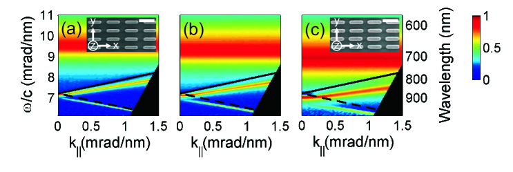
Figure 1: (Color online) Experimental extinction spectra as a function of the wave vector component parallel to the surface of the array. Scanning electron microscope images of the nanorod arrays yielding the spectra in Figures (a) and (c) are shown in the corresponding insets; the scale bar denotes 500 nm. The black solid and dashed lines indicate the $(+1,0)$ and $(-1,0)$ Rayleigh anomalies, respectively. The incident light is polarized parallel to the width of the nanorods (y-direction), which is (a) 85 nm, (b) 95nm, and (c) 115 nm. The broad, dispersionless resonance on the high frequency side of each spectrum is the dipolar localized surface plasmon resonance along the width of the nanorods. The narrower and dispersive resonances below the Rayleigh anomalies are the surface lattice resonances.

We have investigated experimentally three $3\times 3$ mm² arrays of gold nanorods fabricated on a silica substrate using Substrate Conformal Imprint Lithography (SCIL) Verschuuren (2010). The arrays were embedded in a uniform surrounding medium by placing a silica superstrate preceded by n=1.45 index matching fluid to ensure good optical contact. The three arrays have lattice constants $a_{x}=600$ nm and $a_{y}=300$ nm, but they comprise nanorods which differ in size. The nanorods have an approximately rectangular shape in the plane of the array, and a height $=38\pm 2$ nm. The rod size (length $\times$ width) was tuned by varying the exposure dose of the electron beam when preparing the master for nanoimprint. This procedure yielded rods of size (a)$420\times 85$ nm², (b)$430\times 95$ nm², and (c)$450\times 115$ nm², which correspond to the measurements in Figures 1(a),  1(b), and 1(c), respectively. The tolerances of these in-plane dimensions are on the order of $\pm 10$ nm. Figures 1(a) and 1(c) show a Scanning Electron Microscope (SEM) image of the corresponding array, and a cartesian triad in the inset which we use to describe the measurements next.

Figure 1 shows the extinction, defined as $1-T$ with $T$ the zeroth order transmittance, for the three arrays described above. The extinction is displayed as a function of the reduced frequency, i.e., the angular frequency normalized by the speed of light in vacuum, and the component of the incident wave vector parallel to the surface, which is given by $k_{\|}=\frac{\omega}{c}n\sin(\theta)\hat{x}$, with $n$ the refractive index of silica and $\theta$ the angle of incidence. The sample was rotated around the y-axis while the y-polarized collimated beam from a halogen lamp impinged onto the sample, probing the short axis of the nanorods. The broad, dispersionless extinction peak seen on the high frequency side of the spectra for all three arrays corresponds to the excitation of Localized Surface Plasmon Resonances (LSPRs) in the individual nanorods. The black solid and dashed lines indicate the (+1,0) and (-1,0) Rayleigh anomalies of the arrays, respectively. The Rayleigh anomalies are solutions to the equation $k_{out}^{2}=k_{in}^{2}$ sin${}^{2}(\theta)+m_{1}^{2}(2\pi/a_{x})^{2}+m_{2}^{2}(2\pi/a_{y})^{2}+2k_{in}$ sin$(\theta)m_{1}(2\pi/a_{x})$, where $k_{in}$ and $k_{out}$ are the modulus of the incident and scattered wave vectors and $m_{j}$ ($j=1,2$) are the integers defining the order of diffraction. Physically, these so-called anomalies represent the frequency and wave vector for which the corresponding diffracted orders are propagating grazing to the surface of the array. The coupling of LSPRs to the Rayleigh anomalies gives rise to the SLRs, which manifest in the measurements as narrow and dispersive peaks in extinction at slightly lower frequencies than the associated Rayleigh anomalies.

Figures 1(a)-(c) show the gradual opening of a stop-gap in the dispersion relation of SLRs as the nanorod width increases. The gap is centered near 7 mrad/nm in Fig. 1(a), but its central frequency is lowered and its width $\Delta\omega_{gap}$ increases as the nanorods become wider. We note that this is not a complete photonic band-gap, since it only exists for light polarized parallel to the short axis of the nanorods and with an in-plane wave vector component parallel to the long axis of the nanorods. For light polarized parallel to the long axis of the nanorods, the dipolar LSPR lies at lower energies than the ($\pm$1, 0) diffraction orders at normal incidence, which results in a weak diffractive coupling Auguié and Barnes (2008). On the other hand, for an in-plane wave vector component parallel to the short axis of the nanorods, the ($\pm$1,0) Rayleigh anomalies are degenerate, leading to degenerate ($\pm$1,0) SLRs and therefore no gap Giannini et al. (2010).

Inspired by previous work explaining electromagnetic resonance phenomena in terms of coupled oscillators Garrido Alzar et al. (2002); Mukherjee et al. (2010), we recently introduced an analog to the plasmonic crystal consisting of three mutually coupled harmonic oscillators Rodriguez et al. (2011). In this analogy, the conduction electrons in the nanorod driven by the electromagnetic field are modeled as oscillator 1 driven by a harmonic force $F=F_{0}e^{-i\omega_{s}t}$. The (+1,0) and (-1,0) Rayleigh anomalies are modeled by oscillators 2 and 3, respectively. The equations of motion of the coupled system are,

$$\ddot{x}_{1}+\gamma_{1}\dot{x}_{1}+\omega_{1}^{2}x_{1}-\Omega_{12}^{2}x_{2}-\Omega_{13}^{2}x_{3} =F,$$

$$\ddot{x}_{2}+\gamma_{2}\dot{x}_{2}+\omega_{2}^{2}x_{2}-\Omega_{12}^{2}x_{1}-\Omega_{23}^{2}x_{3} =0,$$ (1)

$$\ddot{x}_{3}+\gamma_{3}\dot{x}_{3}+\omega_{3}^{2}x_{3}-\Omega_{13}^{2}x_{1}-\Omega_{23}^{2}x_{2} =0,$$

with $x_{j}$, $\gamma_{j}$ , and $\omega_{j}$ ($j=1,2,3$) the displacement from equilibrium position, damping, and eigenfrequency associated with the $j^{th}$ oscillator, respectively, and $\Omega_{jk}$ ($k=1,2,3$ and $j\neq k$) the coupling frequency between the $j^{th}$ and $k^{th}$ oscillator. The absorbed mechanical power by oscillator 1 from the driving force, given by $P(t)=F\dot{x}_{1}$, is representative of the extinct optical power by the array. Integrating $P(t)$ over one period of oscillation and scanning the driving frequency $\omega_{s}$ yields an absorbed power spectrum, which we compare to the extinction measurements.

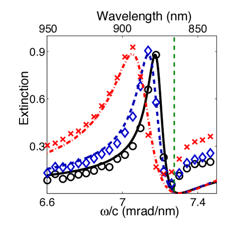
Figure 2: (Color online) The black open circles, blue open diamonds, and red crosses, are the experimental extinction spectra at normal incidence for arrays of nanorods of width 85 nm, 95nm, and 115 nm, respectively. The black solid, blue dashed, and red dash-dot curves are calculations of the absorbed power in the coupled oscillator model described in the text and with fitting parameters as given in Figure 3(c). The dashed vertical line indicates the eigenfrequency $\omega_{2}=7.3$ mrad/nm representing the Rayleigh anomaly in the oscillator model.

Figure 2 displays the extinction spectra for the three arrays at normal incidence, together with calculations done with the coupled oscillator model as fits to the measurements. Only the (+1,0) SLR appears in the spectra, so the model reduces to two oscillators, i.e., $\Omega_{13}=\Omega_{23}=0$. The third oscillator is uncoupled because the (-1,0) SLR is a dark state at normal incidence. This condition arises due to an antisymmetric (quadrupolar) character of the (-1,0) modal fields, which results in a vanishing extinction at normal incidence Rodriguez et al. (2011). Figure 1 shows that for an increasing nanorod width the LSPR displays a diminishing center frequency and a broader linewidth. This behavior is associated with increased retardation and radiative damping Maier (2007), which we model in the calculations of Fig. 2 by lowering $\omega_{1}$ and increasing $\gamma_{1}$. The eigenfrequency of oscillator 2, representing the Rayleigh anomaly frequency, is set to $\omega_{2}=7.3$ mrad/nm for all three cases. In order to unambiguously demonstrate the critical role of the coupling between LSPRs and the Rayleigh anomaly in determining the SLR lineshape, we set the damping of oscillator 2 (whose coupling gives rise to the SLR) equal in all three cases, given by $\gamma_{2}=0.001$ mrad/nm. Considering that the losses are expected to increase for the bigger nanorods, this is unlikely the exact case in the experiments. However, as we show next, fixing $\gamma_{2}$ allows us to see the effect of changing the coupling frequency $\Omega_{12}$, which stands for the radiative coupling strength between the LSPR and the Rayleigh anomaly.

The measurements in Fig. 2 show two main effects on the SLR lineshape as the width of the nanorods increases: i) the peak resonance frequency is increasingly detuned from the Rayleigh anomaly, and ii) the linewidth broadens. As it is shown next, this behavior is explained by the change of the coupling constant between the LSPR and the Rayleigh anomaly. In Fig. 3(a) we plot the detuning of the SLR from the Rayleigh anomaly, $\omega_{RA}-\omega_{SLR}$, and the linewidth at Full-Width Half Maximum (FWHM) of the SLR as a function of the width of the nanorods. It is remarkable that these two quantities are in quantitative agreement, which indicates a direct connection between radiative losses and the peak resonance frequency with respect to the corresponding Rayleigh anomaly. The implications of this connection for sensing small changes to the bulk refractive index by means of plasmonic nanoparticle arrays have been recently discussed Offermans et al. (2011). A universal scaling of the figure of merit of plasmonic sensors, which is a function of the detuning $\omega_{RA}-\omega_{SLR}$ alone, was therein found. In Fig. 3(b) we plot $\omega_{RA}-\omega_{LSPR}$ as a function of the nanorod width, which displays the diminishing frequency difference between the LSPR and the Rayleigh anomaly. This decrease in the magnitude of $\omega_{RA}-\omega_{LSPR}$ with a simultaneous broadening of the LSPR promotes a stronger radiative coupling of localized surface plasmons to diffracted orders, i.e., an increase in $\Omega_{12}$. Figure 3(c) shows the values of $\Omega_{12}$ used to fit the measurements in Fig. 2. Although in the fitted range $\Omega_{12}$ may well be described by a linear function, we have used a quadratic function for a reason that will be clarified further in the text. We see that increasing $\Omega_{12}$ detunes the SLR from the Rayleigh anomaly and broadens it in the right amount to have an excellent agreement with the measurements. A crucial understanding in attributing the observed behavior to $\Omega_{12}$ mainly lies in the fact that changing $\gamma_{2}$ (the intrinsic damping of oscillator 2) can not lead to the right detuning $\omega_{RA}-\omega_{SLR}$. We have verified this through several calculations (not shown here) in which $\gamma_{2}$ and $\Omega_{12}$ were varied independently and/or simultaneously. Next, we consider the more general case of inclined incidence light, where the three oscillators are mutually coupled.

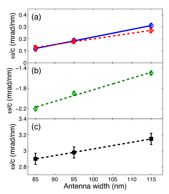
Figure 3: (Color online) Figure (a) shows the (+1,0) SLR linewidth at Full-Width Half Maximum (FWHM) as blue open circles, and the detuning of the SLR from the Rayleigh anomaly, $\omega_{RA}-\omega_{SLR}$, as red open triangles. Both quantities are taken from the extinction measurements at normal incidence. The solid and dashed lines are guides to eye for the FWHM and detuning, respectively. Figure (b) shows the frequency difference between the Rayleigh anomaly and the Localized Surface Plasmon Resonance (LSPR), $\omega_{RA}-\omega_{LSPR}$, as green open diamonds. The green dashed line is a guide to eye. Figure (c) shows the coupling frequency $\Omega_{12}$ used in the coupled oscillator model to calculate the spectra shown in Figure 2. The black dashed curve is a quadratic fit to $\Omega_{12}$. All quantities in (a) and (b) are plotted as a function of the nanorod width. The error bars in (a) and (b) stem from the resolution in the spectrometer, whereas the error bars in (c) represent the uncertainty in the fitting.

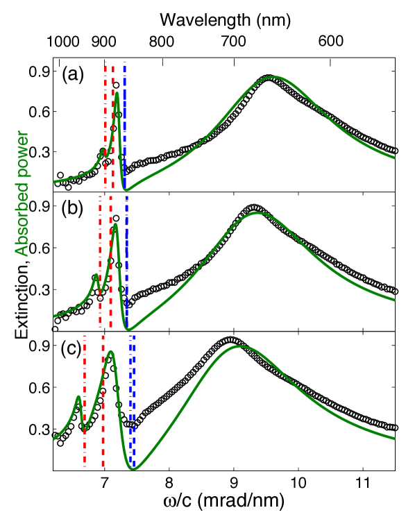
Figure 4: (Color online) The black open circles are cuts of the measured extinction spectra for the three arrays in Figure 1, following the same labeling convention for the antenna width, i.e., (a) 85 nm, (b) 95 nm, and (c) 115 nm. For each case the extinction is shown at the slowdown value of $k_{\|}$, which is at (a) $k_{\|}=0.13$ mrad/nm, (b) $k_{\|}=0.18$ mrad/nm, and (c) $k_{\|}=0.35$ mrad/nm. The green solid curves represent the absorbed power in the coupled oscillator model described in the text, with coupling and damping frequencies as given in Table 1. The blue and red dashed lines are the (+1,0) and (-1,0) Rayleigh anomalies as predicted by the theory (conservation of the parallel component of the wave vector across the interface), respectively. The blue and red dash-dot lines are the eigenfrequencies $\omega_{2}$ and $\omega_{3}$, respectively, set in the oscillator model to calculate the absorbed power spectrum for each case.

Inspection of Fig. 1 points towards the connection between the formation of standing waves in the high frequency SLR band and the opening of the gap. We consider the gap to open at the slowdown point for the high frequency band, i.e., where the dispersion of the (+1,0) SLR flattens and the group velocity slows down to zero. Figure 4 shows the extinction of the three arrays at the slowdown point, which occurs at (a) $k_{\|}=0.13$ mrad/nm, (b) $k_{\|}=0.18$ mrad/nm, and (c) $k_{\|}=0.35$ mrad/nm. In the same Figure we plot the absorbed power spectra for the oscillator model fitting each measurement. From the frequency and linewidth of the dispersionless LSPR we set the eigenfrequency and damping of oscillator 1 to (a) $\omega_{1}=9.5$ mrad/nm, $\gamma_{1}=2.3$ mrad/nm, (b) $\omega_{1}=9.2$ mrad/nm, $\gamma_{1}=2.4$ mrad/nm, and (c) $\omega_{1}=8.8$ mrad/nm, $\gamma_{1}=2.7$ mrad/nm. The coupling and damping frequencies used to fit the SLR lineshapes are given in Table 1, together with the eigenfrequencies $\omega_{2}$ and $\omega_{3}$ representing the Rayleigh anomalies. The blue and red dashed vertical lines in Fig. 4 indicate the (+1,0) and (-1,0) Rayleigh anomalies, respectively, as predicted by the equation describing the conservation of the wave vector component parallel to the surface of the grating. These are the frequencies at which the black lines in the dispersion diagrams in Fig. 1 cross the value of $k_{\|}$ inspected in cases (a)-(c). The blue and red dash-dot vertical lines in Fig. 4 indicate where the dips in extinction associated with the Rayleigh anomalies are seen in the experiment, which are also the eigenfrequencies used in the oscillator model. We see in Fig. 4 that as the nanorod widens and the gap opens there is an increased frequency deviation of the extinction dip with respect to the corresponding theoretically predicted Rayleigh anomalies. Figure 2 displays the same phenomenon for normal incidence light, but the effect is much less pronounced than at the slowdown point. A small shift between the diffraction edge and the associated extinction dip was also observed by Augié and Barnes in the normal incidence extinction spectra of various metallic nanoparticle arrays Auguié and Barnes (2008), but its origin was not discussed. It is crucial to realize that when deriving the conditions for which a diffracted order propagates grazing to the surface of the grating, i.e. the Rayleigh anomaly equation yielding the black lines in Fig. 1 and the dashed lines in Figs. 2 and 4, the form factor of the grating is not considered. The derivation follows from equating the incoming and outgoing wave vectors, the former including the momentum added by the grating. However, this first order analysis neglects any changes in momentum that could arise from the dimensions of the particles constituting the grating. Since the dimensions of the individual particles determine their polarizability, i.e., the frequency and damping of the associated LSPR, we propose that the small shift in frequency of the extinction dip with respect to the corresponding theoretically predicted Rayleigh anomaly may be rooted in the coupling strength of LSPRs to diffracted orders. Indeed, we observe in Figs. 1, 2 and 4 that for the widest nanorods, where the coupling strength of the LSPR to the ($\pm$ 1,0) Rayleigh anomalies is highest, the aforementioned shift is also highest.

Table 1: Coupling and damping frequencies used in equation 1 to reproduce the spectra shown in Figure 4. In the entries for which a minimum estimate is given, the value in parenthesis is the value used in the model yielding the spectra in Figure 8. All quantities are given in units of mrad/nm

	$\omega_{2}$	$\omega_{3}$	$\Omega_{12}$	$\Omega_{13}$	$\Omega_{23}$	$\gamma_{2}$	$\gamma_{3}$
$k_{\|}$=0.13	7.31	7.01	3.0 $\pm$ 0.1	$<1.0$ (0.4)	$1.0\pm 0.1$	$<0.02$ (0.008)	$0.08\pm 0.03$
$k_{\|}$=0.18	7.34	6.93	3.2 $\pm$ 0.1	$<1.0$ (0.5)	$1.2\pm 0.1$	$<0.02$ (0.008)	$0.08\pm 0.02$
$k_{\|}$=0.35	7.40	6.69	3.5 $\pm$ 0.1	$<1.0$ (0.8)	$1.5\pm 0.1$	$<0.02$ (0.008)	$0.08\pm 0.01$

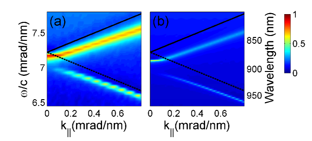
Figure 5: (Color online) Figure (a) is a zoom into the stop-gap displayed in the measurements of Figure 1(a). Figure (b) shows FDTD simulations results for an array of comparable antennas. The extinction is displayed by the same color scale for both measurements and simulations. The black solid and dashed lines represent the (+1,0) and (-1,0) Rayleigh anomalies, respectively.

In order to investigate the properties of the gap for a broader range of nanorod widths, we have performed Finite Difference in Time Domain (FDTD) simulations with an in-house developed software. We have calculated dispersion relations in extinction for arrays with lattice constants $a_{x}=600$ nm and $a_{y}=300$ nm, and rods of dimensions $L=450$ nm, $h=40$ nm. The width of the rods was varied between $w=20$ nm and $w=280$ nm, in steps of 20 nm. Although the three experimental arrays displayed a small change in the length of the nanorods, the dominant contribution to the properties of the gap stems from the width of the nanorod (within the range of length variation). This assumption is based on the fact that the coupled surface modes herein discussed arise for light polarized parallel to the width of the nanorods, and the associated LSPR red-shifts as the width increases, which is the expected behavior due to the depolarization field along this dimension Maier (2007). We validate the simulation results in Fig. 5, where we compare the measured and calculated dispersion relations near the gap for an array of gold nanorods of 80 nm width in both cases. From the dimensions of the three experimental arrays previously given, it can be recognized that the nanorods in the simulations are about $7\%$ shorter in length. Nevertheless, a good qualitative agreement is observed between measurements and simulations.

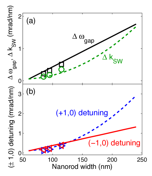
Figure 6: (Color online) Figure (a) shows the frequency width of the stop-gap, $\Delta\omega_{gap}$, and the $k_{\|}$ width of the standing waves in the high frequency SLR band, $\Delta k_{SW}$. The black open squares and solid line represent measurements and FDTD simulations results, respectively, for $\Delta\omega_{gap}$. The green open circles and dashed curve represent measurements and FDTD simulations results, respectively, for $\Delta k_{SW}$. Figure (b) shows the detuning of the ($\pm$1,0) SLRs from their respective Rayleigh anomalies. The (-1,0) detuning is plotted with red left-pointing triangles and a solid line, for measurements and FDTD simulations results, respectively. The (+1,0) detuning is plotted with blue right-pointing triangles and a dashed curve, for measurements and FDTD simulations results, respectively. All quantities in (a) and (b) are plotted as a function of the nanorod width.

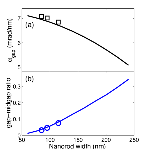
Figure 7: (Color online) Figure (a) shows the central frequency of the stop-gap, $\omega_{gap}$, with black open squares representing measurements and a black solid curve representing FDTD simulation results. Figure (b) shows the gap-midgap ratio, with blue open circles representing measurements and a blue solid curve representing FDTD simulations results. All quantities in (a) and (b) are plotted as a function of the nanorod width.

In Fig. 6(a) we plot the frequency width of the stop-gap, $\Delta\omega_{gap}$, and the $k_{\|}$ width of the standing waves in the high frequency SLR band, $\Delta k_{SW}$, both as function of the width of the nanorods. $\Delta\omega_{gap}$ is taken to be the frequency difference between the slowdown point and the (-1,0) SLR, both evaluated at the $k_{\|}$ value of the slowdown point. $\Delta k_{SW}$ is equal to the value of $k_{\|}$ at the slowdown point. In Fig. 6(b) we plot the detuning of the ($\pm 1,0$) SLRs from their respective theoretically predicted Rayleigh anomalies, also as a function of the nanorod width. The open data points are taken from the measurements of the three arrays, and the solid and dashed curves result from the simulations. A central finding is that both $\Delta\omega_{gap}$ and the (-1,0) detuning are linearly increasing functions of the nanorod width, while $\Delta k_{SW}$ and the (+1,0) detuning are both quadratically increasing functions of the nanorod width. We therefore find the frequency width of the gap to be correlated with the (-1,0) detuning, and the $k_{\|}$ width of the standing waves to be correlated with the (+1,0) detuning. In terms of the coupled oscillator model, this can be interpreted as follows: the gap opens with a linear increase in $\Omega_{13}$ (coupling of LSPR to the (-1,0) order), whereas the in-plane momentum width of the standing waves broadens with a quadratic increase in $\Omega_{12}$ (coupling of LSPR to the (+1,0) order). The latter dependance is the reason for which $\Omega_{12}$ was fitted with a quadratic function in the normal incidence spectra, i.e., the dashed curve in Fig. 3(c).

Further quantifying the properties of the gap, in Fig. 7(a) we plot the central frequency of the stop-gap, $\omega_{gap}$, which falls quadratically for increasing nanorod width. In Fig. 7(b) we plot the gap-midgap ratio, $\Delta\omega_{gap}/\omega_{gap}$ which rises quadratically for increasing nanorod width. Figure 7(a)shows that for nanorods wider than those considered in the experiments, the central frequency of the gap falls into the infrared part of the spectrum. Limited by the spectral response of our acquisition system (based on a silicon detector), we are unable to perform measurements for the wider nanorods. Nevertheless, in light of the good agreement between measurements and simulations we believe Figs. 6(a) and  7 accurately encompass all properties of the gap as function of the nanorod width, and provide a suitable recipe upon which stop gaps in plasmonic crystals may be opened and tuned. Comparing to previous work, where it was found that the gap’s width is a linearly increasing function of the modulation amplitude in metallic sinusoidal gratings Barnes et al. (1996), we have also found a linear dependance of the gap’s width on a single structural factor. However, the connection between these two works is not an obvious one, since whereas Barnes and co-workers have varied a dimension out of the plane of propagation, we have investigated structures of equal height but variable dimensions in the plane of propagation. From a fabrication point of view, a precise in plane structuring of plasmonic crystals may offer a higher degree of versatility in how stop-gaps may be tuned and at a greater ease.

We now discuss the validity range of the previously discussed SLR properties on the nanorod width. Figure 8 shows the extinction of two arrays with lattice constants $a_{x}=600$ nm, $a_{y}=300$ nm, nanorods of length$=450$ nm and height $=40$ nm, and embedded in a homogeneous environment of n=1.45; these conditions are the same as in the experiments presented in Fig. 1. The width of the nanorods in Fig. 8 is (a) 60 nm, and (b) 240 nm, which correspond to the extremes of the curves plotted in Figs. 6 and 7. Due to the very different extinction efficiency of the two arrays in the spectral region of interest, the extinction is displayed by a logarithmic color scale common to both graphs, which allows quantitative comparison of the spectra. The low extinction and remarkably narrow resonances seen in Fig. 8(a) can be explained in terms of the coupled oscillator model as a consequence of the low coupling strength of LSPRs to diffracted orders. This point can be inferred from the quantities given in Table 1, where all coupling frequencies $\Omega_{jk}$ are seen to decrease as the nanorod width decreases. Lower $\Omega_{12}$ and $\Omega_{13}$ therefore translate into a lower coupling strength of LSPRs to diffracted orders, whereas a lower $\Omega_{23}$ translates into a lower coupling between the (+1,0) and (-1,0) SLRs and therefore a smaller gap. As the width of the nanorods increases and the $\Omega_{jk}$ terms increase, the extinction at the SLRs also increases, the resonance linewidth broadens, and the frequency gap widens, eventually reaching the case displayed in Fig. 8(b) for a nanorod width of $240$ nm. Figure 8(b) displays a dipolar LSPR near 6.8 mrad/nm, which is lower in frequency than the diffraction edge at normal incidence. The (+1,0) SLR can still be recognized in the spectrum from the non-dispersive feature near 6.0 mrad/nm (in the red tail of the LSPR). However, for wider nanorods the LSPR shifts to lower frequencies, thereby making the (+1,0) SLR indistinguishable from the LSPR. As the energy of the dipolar LSPR becomes substantially lower that the ($\pm 1,0$) diffraction orders, diffractive coupling of dipolar LSPRs becomes very weak, and the properties of coupled SLRs leading to the opening of the stop-gap significantly deviate.

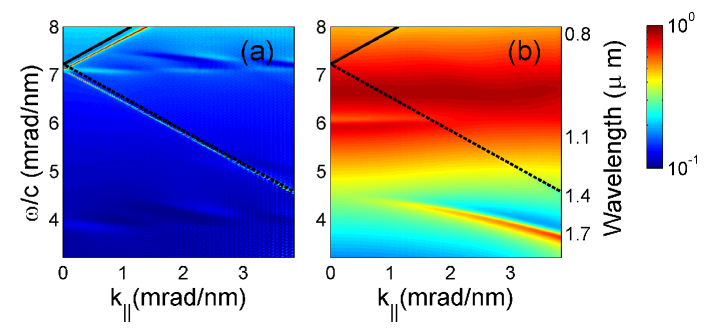
Figure 8: (Color online) FDTD simulations results for the extinction of an array of gold nanorods of width (a) 60 nm and (b) 240 nm. Both arrays have nanorods of length = 450 nm, height = 40 nm, in a lattice with constants $a_{x}=600$ nm and $a_{y}=300$ nm. The black solid and dashed lines indicate the (+1,0) and (-1,0) Rayleigh anomalies, respectively. The extinction is displayed by a logarithmic color scale common to both graphs.

In conclusion, we have shown how the radiative coupling strength of localized surface plasmons to diffracted orders in periodic arrays of nanorods can be tuned. This tuning is achieved experimentally by modifying the width of the nanorods, and results in the opening of frequency stop-gaps whose properties are therefore tunable. A quadratic dependence of both the frequency width of the stop-gap and the (-1,0) SLR detuning was found on the nanorod width. A linear dependence of both the in-plane momentum width of the standing waves in the high-frequency SLR band and the (+1,0) SLR detuning was found on the nanorod width. In light of a coupled oscillator analog to the plasmonic crystal, we have associated these two correlations with the coupling strength of localized surface plasmons to the (-1,0) and (+1,0) diffracted orders. Supporting experiments with numerical simulations for a wider set of nanorod widths, we have analyzed the properties of the gap and discussed the limiting cases where the scaling laws we present deviate. Although we have only considered nanorod arrays in this work, similar results are expected to hold in periodic arrays of particles with different geometries whereby diffractive coupling of localized surface plasmons is possible. Our results therefore pave the road towards nanoscale light manipulation in 2D plasmonic crystals, since stop-gaps allow to selectively enhance or suppress light-matter interactions.

We thank M. Verschuuren for assistance in the fabrication of the samples, and G. Lozano for fruitful discussions. This work was supported by the Netherlands Foundation Fundamenteel Onderzoek der Materie (FOM) and the Nederlandse Organisatie voor Wetenschappelijk Onderzoek (NWO), and is part of an industrial partnership program between Philips and FOM.

References

- Joannopoulos et al. (2008) J. D. Joannopoulos, S. G. Johnson, J. N. Winn, and R. D. Meade, Photonic Crystals: Molding the Flow of Light (Princeton University Press, New Jersey, USA, 2008), 2nd ed.
- Kitson et al. (1996) S. C. Kitson, W. L. Barnes, and J. R. Sambles, Phys. Rev. Lett. 77, 2670 (1996).
- Barnes et al. (1996) W. L. Barnes, T. W. Preist, S. C. Kitson, and J. R. Sambles, Phys. Rev. B 54, 6227 (1996).
- Lochbihler (1994) H. Lochbihler, Phys. Rev. B 50, 4795 (1994).
- Yoon et al. (2003) J. Yoon et al., J. Appl. Phys. 94, 123 (2003).
- Sauvan et al. (2008) C. Sauvan, C. Billaudeau, S. Collin, N. Bardou, F. Pardo, J.-L. Pelouard, and P. Lalanne, Appl. Phys. Lett. 92, 011125 (2008).
- Billaudeau et al. (2008) C. Billaudeau, S. Collin, C. Sauvan, N. Bardou, F. Pardo, and J.-L. Pelouard, Opt. Lett. 33, 165 (2008).
- Ropers et al. (2005) C. Ropers, D. J. Park, G. Stibenz, G. Steinmeyer, J. Kim, D. S. Kim, and C. Lienau, Phys. Rev. Lett. 94, 113901 (2005).
- Ghoshal et al. (2009) A. Ghoshal, I. Divliansky, and P. G. Kik, Appl. Phys. Lett. 94, 171108 (2009).
- Auguié and Barnes (2008) B. Auguié and W. L. Barnes, Phys. Rev. Lett. 101, 143902 (2008).
- Chu et al. (2008) Y. Chu, E. Schonbrun, T. Yang, and K. B. Crozier, Appl. Phys. Lett. 93, 181108 (2008).
- Kravets et al. (2008) V. G. Kravets, F. Schedin, and A. N. Grigorenko, Phys. Rev. Lett. 101, 087403 (2008).
- Vecchi et al. (2009) G. Vecchi, V. Giannini, and J. Gómez Rivas, Phys. Rev. B 80, 201401 (2009).
- Bitzer et al. (2009) A. Bitzer, J. Wallauer, H. Merbold, H. Helm, T. Feurer, and M. Walther, Opt. Exp. 17, 22108 (2009).
- Rodriguez et al. (2011) S. R. K. Rodriguez, A. Abass, B. Maes, O. T. A. Janssen, G. Vecchi, and J. Gómez Rivas (2011), eprint arXiv:1108.1620v1.
- Verschuuren (2010) M. A. Verschuuren, Ph.D. thesis, Utrecht University (2010).
- Giannini et al. (2010) V. Giannini, G. Vecchi, and J. Gómez Rivas, Phys. Rev. Lett. 105, 266801 (2010).
- Garrido Alzar et al. (2002) C. L. Garrido Alzar, M. A. G. Martinez, and P. Nussenzveig, Am. J. Phys. 70, 37 (2002).
- Mukherjee et al. (2010) S. Mukherjee, H. Sobhani, J. B. Lassiter, R. Bardhan, P. Nordlander, and N. J. Halas, Nano Lett. 10, 2694 (2010).
- Maier (2007) S. A. Maier, Plasmonics: Fundamentals and Applications (Springer, New York, USA, 2007).
- Offermans et al. (2011) P. Offermans, M. C. Schaafsma, S. R. K. Rodriguez, Y. Zhang, M. Crego-Calama, S. H. Brongersma, and J. Gómez Rivas, ACS Nano 5, 5151 (2011).