Abstract

The high-energy behavior of ${\cal N}\!=\!4$ SYM elastic amplitudes at strong coupling is studied by means of the AdS/CFT correspondence. We consider the eikonal method proposed by Janik and one of the authors, where the relevant minimal surface is a “generalized helicoid” in hyperbolic space (“Euclidean $AdS_{5}$”), from which the physical amplitude is obtained after an appropriate analytic continuation. We then compare our results with those obtained, using a minimal surface in $AdS_{5}$ momentum space, by Alday and Maldacena for gluon-gluon scattering, and by Barnes and Vaman for quark-quark scattering (“Alday-Maldacena approach”). Exploiting a conformal transformation, we show that the eikonal amplitudes are dominated by the Euclidean version of the cusp contribution found in the Alday-Maldacena approach. The amplitudes in the two approaches are of Regge type at high-energy and with the same logarithmic Regge trajectory independently of the kind of colliding particles, in agreement with the expected universality of Regge trajectories.

1 Introduction

The AdS/CFT correspondence [1] is a powerful non-perturbative tool, which has been exploited in the study of a variety of problems in ${\cal N}\!=\!4$ supersymmetric Yang-Mills theory (SYM) at strong coupling. In recent years, a lot of work has been done regarding scattering amplitudes. In Refs. [2, 3], Alday and Maldacena have shown how to obtain the $n$-gluon scattering amplitude in ${\cal N}\!=\!4$ SYM in this framework, by finding a minimal surface, corresponding to a classical string solution, with polygonal boundary in $AdS_{5}\times S^{5}$. In particular, they have solved analytically the minimal surface problem in the four-gluon case [2], so obtaining a fully analytic expression for the gluon-gluon elastic scattering amplitude. Their method has been extended to quark-quark scattering in Refs. [4, 5, 6]. In these works, quarks are introduced as ${\cal N}\!=\!2$ hypermultiplets on the field theory side, thus modifying the dynamical content of the theory, which requires the introduction of extra structure, namely D7-branes, in the dual gravitational description. The D7-branes are then treated in the probe approximation, neglecting their backreaction, which corresponds to compute the field theory amplitudes in the quenched approximation, i.e., treating the quarks as external probes. In particular, the authors of Ref. [6] obtain an exact solution to the minimal surface problem relevant to quark-quark elastic scattering, and although the area of the surface cannot be expressed in closed form, an explicit expression can be obtained in the limit of small quark masses.

A different method to compute scattering amplitudes through the AdS/CFT correspondence had been previously proposed in Refs. [7, 8, 9], in order to evaluate the high-energy scattering amplitude for external quarks. This method is based on the eikonal approximation and the Wilson-line formalism for high-energy amplitudes [10, 11, 12, 13], and on analytic continuation to Euclidean space [14, 15, 16, 17]. In this case, no new dynamical degree of freedom is added on the field theory side, so that no extra structure has to be introduced in the dual gravitational description. Quarks are treated directly from the onset as external particles coupled to the gauge (and scalar) fields of the ${\cal N}=4$ theory. In this approach, the scattering amplitude is obtained from the correlation function of two Wilson lines running along the eikonal trajectories of the quarks. Through analytic continuation and gauge/gravity duality, this correlation function is related to the area of a minimal surface in Euclidean $AdS_{5}$ (i.e., hyperbolic space), whose boundaries are two straight lines, corresponding to the Euclidean trajectories of the quarks. The relevant minimal surface thus corresponds to a “generalized helicoid” [8] in the AdS background, characterized by the impact-parameter distance between the quarks and by the opening angle $\theta$ of the boundary. After analytic continuation back into Minkowski space, one obtains the impact-parameter amplitude at given high enough rapidity $\chi$. However, the expressions obtained in [8] were not complete, suffering from the lack of knowledge on the exact analytic form of the “generalized helicoid”. One goal of the present paper is to go further in the eikonal approach, in order to go beyond the approximations made in [8], and so obtain a more refined result.

One major interest of the eikonal method is that it can be extended to non-conformal backgrounds [8, 9, 18], corresponding to generic non-conformal gauge field theories, where using general features of gauge/gravity duality it leads in this case to Regge amplitudes with linear trajectory. Our aim in the present study is to look for Regge behavior of amplitudes in the conformal case of ${\cal N}\!=\!4$ SYM by using this method.

Indeed, the high-energy behavior of scattering amplitudes has been analyzed for a long time in terms of Regge amplitudes, both from the phenomenological and the theoretical point of view (see e.g. Ref. [19]). As it is well known, the Regge behavior is a remarkable property of Yang-Mills theories in the perturbative regime. However, the issue of Regge behavior of high-energy amplitudes at strong coupling requires different tools, and the AdS/CFT correspondence seems to be well suited for this purpose. In the case of gluon-gluon scattering, the analysis of the high-energy behavior has been carried out in Refs. [20, 21], based on the Alday-Maldacena result of Ref. [2], and on dual conformal symmetry [22] and the all-order BDS ansätz of Ref. [23], showing indeed the Regge nature of the amplitude (which in particular is Regge-exact in the $s$-channel [21]). This analysis can be easily extended to the results of Ref. [6], which will allow us to discuss the issue of universality of Regge amplitudes in ${\cal N}\!=\!4$ SYM at strong coupling. On the other hand, the comparison with the results obtained in the eikonal approach allows to check the compatibility of the two methods, which are based on very different constructions, and thus provide a nontrivial test for the validity of the eikonal approach. This is very important in view of the application of the eikonal approach to QCD, where an analogue of the Alday-Maldacena approach is not currently available, and moreover allows to look at the universality problem in a different way.

The plan of the paper is the following. In Section 2, we give a brief review of the two methods for approaching the high-energy behavior of ${\cal N}\!=\!4$ SYM amplitudes, namely the Alday-Maldacena approach of Ref. [2], and the eikonal approach of Ref. [8]. In Section 3, we investigate in detail the minimal surface related to gluon-gluon scattering obtained by Alday and Maldacena. In particular, the IR boundary of this solution is analyzed, together with the UV boundary of a corresponding solution in Euclidean $AdS_{5}$, generated by analytic continuation. In Section 4, we investigate the high-energy domain of the Alday-Maldacena gluon-gluon scattering amplitude, both in the momentum and in the impact-parameter representation, making explicit that in this domain the amplitude is of Regge type. Moreover, we compare the result with the quark-quark scattering amplitude of Ref. [6], and discuss the issue of universality of the Regge trajectory. In Section 5, we study the minimal surface problem in Euclidean $AdS_{5}$ relevant to quark-quark scattering in the eikonal method in a new way, which allows us to go beyond the preliminary results of Ref. [8]. In particular, we show that the amplitude is of Regge type, and we obtain the leading behavior of the Regge trajectory, which we show to be in agreement with the trajectory obtained with the Alday-Maldacena method. We also extend the results of the eikonal approach to the gluon-gluon scattering case, finding the agreement expected in the light of universality. Finally, Section 6 is devoted to conclusions and outlook.

2 Two-body elastic scattering via the AdS/CFT correspondence

2.1 The Alday-Maldacena approach

The gluon four-point scattering amplitude in ${\cal N}\!=\!4$ SYM has been evaluated in Ref. [2], making use of the AdS/CFT correspondence, by computing the area of a corresponding minimal surface. In the dual gravity theory, which is defined in $AdS_{5}\times S^{5}$, the gluon-gluon scattering amplitude is mapped into the scattering amplitude of four open strings. In turn, the string amplitude is obtained by determining a minimal surface, corresponding to a classical string solution for the Nambu-Goto action. This minimal surface lives in the $AdS_{5}$ background,

$$ds^{2}={R^{2}\over z^{2}}\big{(}\eta_{\mu\nu}dx^{\mu}dx^{\nu}+dz^{2}\big{)}\,,$$ (2.1)

where $\mu=0,1,2,3$ and $\eta_{\mu\nu}={\rm diag}(-1,1,1,1)$. We call this background the position space. The idea of Ref. [2] is to find the minimal surface in momentum space, rather than directly in the position space. The momentum space $(y^{\mu},r)$ is obtained from the position space $(x^{\mu},z)$ by means of the T-duality transformation,

$$\partial_{m}y^{\mu}=i{R^{2}\over z^{2}}\epsilon_{mn}\partial_{n}x^{\mu}\,,$$ (2.2)

and the resulting metric is given by

$$ds^{2}={R^{2}\over r^{2}}\big{(}\eta_{\mu\nu}dy^{\mu}dy^{\nu}+dr^{2}\big{)}\,,\quad r\equiv{R^{2}\over z}\,.$$ (2.3)

In the momentum space, the boundary of the minimal surface corresponding to the four-gluon amplitude (i.e. to two-body scattering) is given by the closed sequence of four light-like segments $\Delta y_{i}^{\mu}$. The boundary conditions in the position space, i.e., that the vertex-operator insertion point $x_{i}$ carries the momentum $k_{i}$ of the corresponding open string, translates into the condition $\Delta y_{i}=2\pi k_{i}$. In the same way, the gluon $n$-point amplitude is obtained from the minimal surface having as boundary a closed sequence of $n$ light-like segments [3]. The sequences are closed because of momentum conservation. The light-like segments lie at $r=r_{\rm IR}=R^{2}/z_{\rm IR}$, where $z_{\rm IR}$ is the fifth coordinate in position space of the D-brane on which the open strings end. Such a D-brane acts as a regulator for the IR divergencies of the gluon-gluon scattering amplitude, which has to be removed by sending $z_{\rm IR}\to\infty$, i.e., $r_{\rm IR}\to 0$, at the end of the calculation. It is however more convenient to find the minimal surface directly at $r_{\rm IR}=0$, which requires to trade $r_{\rm IR}$ for a different IR regulator when evaluating the area of the surface.

The solution obtained in Ref. [2] for the minimal surface relevant to the gluon four-point scattering amplitude reads in momentum space

$$y_{0} ={\alpha\sqrt{1+\beta^{2}}\sinh u_{1}\sinh u_{2}\over\cosh u_{1}\cosh u_{2}+\beta\sinh u_{1}\sinh u_{2}}\,,$$ (2.4a)

$$y_{1} ={\alpha\sinh u_{1}\cosh u_{2}\over\cosh u_{1}\cosh u_{2}+\beta\sinh u_{1}\sinh u_{2}}\,,$$ (2.4b)

$$y_{2} ={\alpha\cosh u_{1}\sinh u_{2}\over\cosh u_{1}\cosh u_{2}+\beta\sinh u_{1}\sinh u_{2}}\,,$$ (2.4c)

$$y_{3} =0\,,$$ (2.4d)

$$r ={\alpha\over\cosh u_{1}\cosh u_{2}+\beta\sinh u_{1}\sinh u_{2}}\,,$$ (2.4e)

where $u_{1,2}$ are world-sheet coordinates on the surface ranging from $-\infty$ to $+\infty$. The parameters $\alpha,\beta$ are related to the Mandelstam variables $s,t$ as

$$-s\,(2\pi)^{2}={8\alpha^{2}\over(1-\beta)^{2}}\,,\quad-t\,(2\pi)^{2}={8\alpha^{2}\over(1+\beta)^{2}}\,.$$ (2.5)

By the use of the T-dual transformation (2.2), the minimal surface (2.4) is mapped back into the position space as

$$x_{0} ={iR^{2}\over 2\alpha}\sqrt{1+\beta^{2}}(\cosh^{2}u_{2}-\cosh^{2}u_{1})\,,$$ (2.6a)

$$x_{1} ={iR^{2}\over\alpha}\bigg{[}{u_{2}\over 2}+{1\over 4}\sinh 2u_{2}+\beta\bigg{(}-{u_{1}\over 2}+{1\over 4}\sinh 2u_{1}\bigg{)}\bigg{]}\,,$$ (2.6b)

$$x_{2} ={iR^{2}\over\alpha}\bigg{[}-{u_{1}\over 2}-{1\over 4}\sinh 2u_{1}+\beta\bigg{(}{u_{2}\over 2}-{1\over 4}\sinh 2u_{2}\bigg{)}\bigg{]}\,,$$ (2.6c)

$$x_{3} =0\,,$$ (2.6d)

$$z ={R^{2}\over\alpha}(\cosh u_{1}\cosh u_{2}+\beta\sinh u_{1}\sinh u_{2})\,.$$ (2.6e)

Substituting the minimal surface solution (2.4) into the Nambu-Goto action, the gluon-gluon scattering amplitude is evaluated as

$${\cal A}^{\rm gluon} =e^{iS}=\exp\bigg{[}2iS_{\rm div}(s)+2iS_{\rm div}(t)+{\sqrt{\lambda}\over 8\pi}\bigg{(}\log{s\over t}\bigg{)}^{2}+{\tilde{C}}\bigg{]}\,,$$ (2.7)

$$iS_{\rm div}(p)=-{1\over\epsilon^{2}}{1\over 2\pi}\sqrt{\lambda\mu^{2\epsilon}\over(-p)^{\epsilon}}-{1\over\epsilon}{1\over 4\pi}(1-\log 2)\sqrt{\lambda\mu^{2\epsilon}\over(-p)^{\epsilon}}\,,\quad(p=s,t)$$ (2.8)

where ${\tilde{C}}$ is a constant that is irrelevant to our purposes. Here $\lambda$ is the ’t Hooft coupling defined by $\sqrt{\lambda}\equiv\sqrt{g_{\rm YM}^{2}N_{c}}=R^{2}/\alpha^{\prime}$, and we have adopted units where $\alpha^{\prime}=1$. Dimensional regularization has been employed in order to obtain a finite result for the area of the minimal surface, by going to $D=4-2\epsilon$ dimensions (with $\epsilon<0$). This requires the introduction of an IR cutoff scale $\mu$, having dimensions of mass, to account for the mass dimension of the $D$-dimensional coupling. Note that the expression (2.7) agrees with the BDS ansätz [23] in the strong coupling limit.

The approach of Ref. [2] has been extended to the case of quark-quark scattering in Refs. [4, 5, 6]. The scattering amplitude is related to a minimal surface in a modified gravitational background including D7-branes, whose positions in the radial direction of AdS corresponds to the masses of the various flavours of quarks. In particular, Ref. [6] provides an exact solution, although in implicit form, for the minimal surface relevant to elastic quark-quark scattering. An explicit expression for the regularized area is also obtained in the limit of small quark masses, which we will report in Section 4.

2.2 The eikonal approach

Let us recall now some relevant elements of the derivation of the quark-quark elastic scattering amplitude in the high-energy domain, in the framework of the AdS/CFT correspondence, following the eikonal approach of Ref. [8]. The starting point is the formulation of high-energy elastic scattering amplitudes, at fixed and small momentum transfer, in terms of the correlation function ${\cal A}^{qq}$ of two Wilson lines [10, 11, 12, 13],

$${\cal A}^{qq}_{ij,kl}={1\over Z_{W}^{2}}\langle(W_{1}-1)_{ij}(W_{2}-1)_{kl}\rangle\,,\quad Z_{W}={1\over N_{c}}\langle{\rm tr}\,W_{1}\rangle={1\over N_{c}}\langle{\rm tr}\,W_{2}\rangle\,,$$ (2.9)

where $Z_{W}$ is a renormalisation constant, which makes ${\cal A}^{qq}$ UV-finite (see $e.g.$ [14]). The relevant Wilson lines $W_{1,2}$ run along infinite light-like straight lines, at transverse separation $b$, and are taken in the representation appropriate for the particles under consideration. We will be interested initially in the scattering of massive quarks (antiquarks) in the fundamental (anti-fundamental) representation, which we use as external probes of ${\cal N}\!=\!4$ SYM. This approach essentially amounts to consider the eikonal approximation for the elastic amplitude, which is expected to be valid in the Regge kinematic region for ${\cal N}\!=\!4$ SYM (as well as for QCD).

The correlation function (2.9) yields the impact-parameter representation for the elastic scattering amplitudes in the $s$-channel. In order to regularize IR divergencies, the Wilson lines are cut at some proper time $\pm T$, and moved slightly away from the light-cone. In this way, they correspond to the classical trajectories of two massive quarks, which form a finite hyperbolic angle $\chi$, related to the center-of-mass total energy squared $s$ as $\chi\sim\log(s/M^{2})$ at high energy. Here $T$ acts as an IR regulator, which has to be removed at the end of the calculation by taking the limit $T\to\infty$, while the quark mass $M$ is irrelevant in the large $\chi$ region. Explicitly, the quark-quark scattering amplitude is then given by [10, 11, 12, 13]

$${\cal M}^{qq\,\,\alpha^{\prime}\!\alpha,\beta^{\prime}\!\beta}_{ij,kl}(s,t)=\delta_{\alpha^{\prime}\!\alpha}\delta_{\beta^{\prime}\!\beta}{\cal M}^{qq}_{ij,kl}(s,t)=\delta_{\alpha^{\prime}\!\alpha}\delta_{\beta^{\prime}\!\beta}(-2is)\int d^{2}b\,e^{i\vec{q}\cdot\vec{b}}{\cal A}^{qq}_{ij,kl}(\chi,b,T)\,,$$ (2.10)

where $\alpha^{\prime},\alpha$ (resp. $\beta^{\prime},\beta$) are the final and initial spin indices of quark 1 (resp. 2), and $i,j$ (resp. $k,l$) are the final and initial color indices of quark 1 (resp. 2). Moreover, $\vec{q}$ and $\vec{b}$ are two-dimensional vectors in the transverse plane, with $t=-\vec{q}^{\,2}$ and $b=|\vec{b}|$. Here the limits $\chi\to\infty$, $T\to\infty$ are understood.

It has been shown that the Minkowskian Wilson line correlation function ${\cal A}^{qq}(\chi,b,T)$ can be reconstructed from the correlation function ${\cal A}^{qq}_{E}(\theta,b,T)$ of two corresponding Euclidean Wilson lines, by means of analytic continuation [14, 15, 16, 17]. The relevant Euclidean Wilson lines run along straight lines of length $2T$, which form now an angle $\theta$ in Euclidean space, and are separated by the same transverse distance $b$ as in the Minkowskian case. Starting from ${\cal A}^{qq}_{E}$, the quark-quark elastic scattering amplitude in the $s$-channel is obtained by means of the analytic continuation relation [16],

$${\cal A}^{qq}_{ij,kl}(\chi,b,T)={\cal A}_{E\,ij,kl}^{qq}(-i\chi,b,iT)\,,\quad{\cal A}_{E\,ij,kl}^{qq}(\theta,b,T)={\cal A}^{qq}_{ij,kl}(i\theta,b,-iT)\,.$$ (2.11)

Moreover, the impact-parameter amplitude in the crossed $u$-channel ${\cal A}^{q{\bar{q}}}$, corresponding to quark-antiquark scattering at center-of-mass energy squared $u$ ($u>0$), can be obtained through the crossing-symmetry relations [17]

$${\cal A}^{q\bar{q}}_{ij,kl}(\chi,b,T)={\cal A}^{qq}_{ij,lk}(i\pi-\chi,b,T)={\cal A}_{E\,ij,lk}^{qq}(\pi+i\chi,b,iT)={\cal A}_{E\,ij,kl}^{q\bar{q}}(-i\chi,b,iT)\,,$$ (2.12)

where in the last passage ${\cal A}_{E\,ij,kl}^{q\bar{q}}(\theta,b,T)\equiv{\cal A}_{E\,ij,lk}^{qq}(\pi-\theta,b,T)$ is the crossed Euclidean amplitude, and where $\chi$ has to be identified with

$$\chi\sim\log{u\over M^{2}}\sim\log{-s\over M^{2}}$$ (2.13)

in the high-energy limit. This relation will be useful further on, when comparing with the Alday-Maldacena amplitude.

The Euclidean Wilson-line correlation functions can be computed through the AdS/CFT correspondence, following the approach of Ref. [24]. On the field theory side, the fundamental Wilson lines running along straight lines describe the propagation of heavy fundamental particles in Euclidean space. Using the gauge invariance of the vacuum, the Euclidean correlation function ${\cal A}^{qq}$ can be decomposed into a singlet and an “octet” part,

$${\cal A}^{qq}_{E\,ij,kl}={\cal A}_{0}\delta_{ij}\delta_{kl}+{\cal A}_{N_{c}^{2}-1}t^{a}_{ij}t^{a}_{kl}\,,$$ (2.14)

where $t^{a}$ are the generators of $SU(N_{c})$ in the fundamental representation, and simple algebra allows to relate the coefficients of the two color structures to the (normalized) expectation values of the Wilson loops obtained by properly closing the contour at infinity, namely

$${\cal A}_{0} ={1\over Z_{W}^{2}}\bigg{(}{1\over N_{c}^{2}}\langle{\rm tr}\,W_{1}{\rm tr}\,W_{2}\rangle-1\bigg{)}\,,$$ (2.15)

$${\cal A}_{0}+{N_{c}^{2}-1\over 2N_{c}}{\cal A}_{N_{c}^{2}-1} ={1\over Z_{W}^{2}}\bigg{(}{1\over N_{c}}\langle{\rm tr}\,W_{1}W_{2}\rangle-1\bigg{)}\,.$$ (2.16)

We stress the fact that there is no relation between the heavy particles in Euclidean space and the “physical” quarks in Minkowski space: indeed, the Euclidean particles are only introduced as an intermediate device to compute the relevant Wilson-loop expectation values, playing no role in the physical process under consideration. We will return on this point in the following.

Massive particles can be introduced in ${\cal N}\!=\!4$ SYM by breaking the $SU(N_{c}+1)$ symmetry to $SU(N_{c})\times U(1)$, which gives rise to massive $W$-bosons transforming in the fundamental representation of $SU(N_{c})$. On the gravity theory side, this can be accomplished by stretching one of the $N_{c}+1$ branes away from the others, and towards the boundary $z=0$ of Euclidean $AdS_{5}$. The mass of the $W$-bosons is related to the position $z_{B}$ of the displaced brane as $M_{B}\sim z_{B}^{-1}$, and therefore it becomes very large as $z_{B}\to 0$. The Wilson loop describing the propagation of the $W$-bosons along a closed contour ${\cal C}$ is identified in the dual bulk theory as the partition function of a string propagating in Euclidean $AdS_{5}$, with the boundary condition that it ends on the contour ${\cal C}$ at the boundary $z=0$. To leading order, it is therefore given by $\langle{\cal W}\rangle\sim\exp(-A)$ with $A$ the (properly regularized) area of a minimal surface in Euclidean $AdS_{5}$, ending on ${\cal C}$ at the boundary $z=0$. Also in this case it is convenient to work directly in the limit $z_{B}=0$, while at the same time regularizing the area (in the UV) by limiting the integration to the region $z>\epsilon$. UV divergencies are dealt with by means of the Legendre transform prescription of Ref. [25].

A remark is in order here. Since we are considering heavy (Euclidean) particles, the boundary conditions for the minimal surface in the supergravity description of the problem are naturally given at the UV, $z=0$. This is in contrast with the calculation of Ref. [2], where such boundary conditions are given at the IR, $z=\infty$, which is again natural for massless particles. One question we want to answer to is how the two points of view can be reconciled. Let us note that while the computation of Ref. [2] is performed in Minkowski space, here we are considering a calculation in Euclidean space, from which the physical, Minkowskian result for the scattering amplitude is recovered only after analytic continuation. In Euclidean space, the heavy $W$-boson is introduced only to establish a connection between the expectation value of the relevant Wilson loops on the field theory side, and their dual description on the gravity side. In particular, the $W$-boson mass plays only the role of a UV regulator in the computation of the area of the relevant minimal surfaces, and drops from the Wilson-loop expectation values after UV divergencies have been removed, before the analytic continuation. On the other hand, the physical scattering amplitude depends on the mass $M$ of the Minkowskian quarks (and on $s$) only through the dependence of the relevant (Minkowskian) Wilson-loop expectation values on the hyperbolic angle $\chi$. In other words, the dependence on $M$ appears only when the relation between $\chi$, $s$ and $M$ is made explicit after the analytic continuation. This shows that the mass of the Euclidean (heavy) $W$-boson and the mass of the Minkowskian quarks are completely unrelated. We see therefore that there is a natural connection between the use of very heavy particles in Euclidean space, and the final goal of describing the scattering of particles with very high energy in Minkowski space, the link being provided by the use of Wilson loops and by the analytic continuation (2.11).

We specialize now to the case of interest, i.e., the Euclidean correlator ${\cal A}^{qq}_{E}(\theta,b,T)$. First of all, we notice that the normalisation factor reduces to $Z_{W}\sim 1$, due to the Legendre transform prescription [25]. This prescription implies also that the disconnected contributions to the expectation values on the right hand side of Eqs. (2.15) and (2.16) is 1, and therefore gets cancelled. Next, since the connected part of ${\cal A}_{0}$ is related to a minimal surface with tube topology, we have that ${\cal A}_{0}={\cal O}(1/N_{c}^{2})$, and so the amplitude is dominated by the “octet” component ${\cal A}_{N_{c}^{2}-1}$, which is of order ${\cal O}(1/N_{c})$: indeed, the relevant minimal surface in Eq. (2.16) has disk topology, so that the right hand side is of order 1. Finally, we obtain at large $N_{c}$

$${\cal A}^{qq}_{E\,ij,kl}\sim{\cal A}_{N_{c}^{2}-1}t^{a}_{ij}t^{a}_{kl}\sim{1\over N_{c}}\delta_{il}\delta_{jk}{1\over N_{c}}\langle{\rm tr}\,W_{1}W_{2}\rangle_{c}\equiv{1\over N_{c}}\delta_{il}\delta_{jk}\tilde{{\cal A}}^{\rm quark}_{E}\,,$$ (2.17)

where the subscript $c$ stands for the connected component.

The basic building block of the construction is therefore a minimal surface in anti-de Sitter space, which is bounded by two oriented straight lines at the boundary $z=0$ of $AdS_{5}$, corresponding to the trajectories of the two heavy Euclidean quarks in the static (infinite mass) limit. We call this surface a “generalized helicoid”.

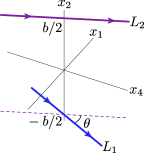
Figure 1: The two straight-line trajectories defining the UV boundary of the minimal surface in the eikonal approach.

In order to properly define the variational problem, it is convenient to take the two lines to have infinite length, while at the same time introducing a new IR cutoff to regularize the area of the resulting minimal surface. In practice, the boundary is defined by the two straight lines

$$L_{1}:\bigg{(}-\tau\sin{\theta\over 2},-{b\over 2},0,\tau\cos{\theta\over 2}\bigg{)}\,,\quad L_{2}:\bigg{(}\tau\sin{\theta\over 2},{b\over 2},0,\tau\cos{\theta\over 2}\bigg{)}\,,\qquad-\infty\leq\tau\leq\infty\,,$$ (2.18)

traveled from $\tau=-\infty$ to $\tau=+\infty$, separated by a distance $b$ in the “transverse” direction $x_{2}$, and forming a relative angle $\theta$ in the “longitudinal” plane $(x_{1},x_{4})$ (see 1). On the other hand, since the area functional

$$A^{\rm quark}_{\theta,b}={\sqrt{\lambda}\over 2\pi}\int d\tau d\sigma{1\over z^{2}}\sqrt{\det\big{(}{\delta_{\mu\nu}\partial_{a}x^{\mu}\partial_{b}x^{\nu}+\partial_{a}z\partial_{b}z}\big{)}}\equiv\int d\tau d\sigma{\cal L}$$ (2.19)

with the boundary (2.18) at $z=0$ is expected to be infinite due to IR divergences, we limit the range of $\tau$ to $\tau\in[-T,T]$, understanding that it has to be imposed in the computation of the area, and not in the determination of the minimal surface. The regularized (and UV-subtracted) area of the surface minimizing the functional (2.19) is therefore a function $A^{\rm quark}_{\rm min}(\theta,b,T)$, which enters the color-independent part of the Euclidean “amplitude”, defined in Eq. (2.17), as $\tilde{{\cal A}}_{E}^{\rm quark}(\theta,b,T)=\exp\big{[}-A^{\rm quark}_{\rm min}(\theta,b,T)\big{]}$. This function will be defined more precisely in Section 5.1.

The case of quark-antiquark scattering is obtained by simply flipping the orientation of one of the two straight lines, e.g.,

$$L_{2}\to L^{\prime}_{2}:\bigg{(}-\tau\sin{\theta\over 2},{b\over 2},0,-\tau\cos{\theta\over 2}\bigg{)}\,,$$ (2.20)

with $\tau$ running again from $-\infty$ to $+\infty$. This corresponds to changing the representation of the corresponding Wilson line from fundamental to anti-fundamental, as appropriate for an antiquark. In turn, exploiting the Euclidean symmetries, it is easy to see that this is equivalent to the change $\theta\to\pi-\theta$ in the relative angle. The minimal surface relevant to quark-antiquark scattering is therefore obtained by minimizing $A^{\rm quark}_{\pi-\theta,b}$, and thus it is equal to $A^{\rm quark}_{\rm min}(\pi-\theta,b,T)$, so that the two cases can be treated at once.

In the case of the $AdS_{5}\times S^{5}$ background one does not know yet the minimal surface corresponding to the boundaries (2.18). A simple scheme has been introduced in Ref. [8], where the following ansätz for the “generalized helicoid” is assumed in order to find the minimal solution,

$$x_{1}=\tau\sin{\theta\sigma\over b}\,,\quad x_{2}=\sigma\,,\quad x_{3}=0\,,\quad x_{4}=\tau\cos{\theta\sigma\over b}\,,\quad z=z(\tau,\sigma)\,.$$ (2.21)

The world-sheet coordinates $\tau,\sigma$ are in the range, $\tau\in[-\infty,\infty]$ and $\sigma\in[-b/2,b/2]$. Using this ansätz, the regularized area functional (2.19) becomes

$$A^{\rm quark}_{\pi-\theta,b}={\sqrt{\lambda}\over 2\pi}\int_{-T}^{T}d\tau\int_{-b/2}^{b/2}d\sigma{1\over z^{2}}\sqrt{\left(1+{{\tau^{2}\theta^{2}}\over{b^{2}}}\right)\big{(}1+(\partial_{\tau}z)^{2}\big{)}+(\partial_{\sigma}z)^{2}}\,,$$ (2.22)

where the IR cutoff parameter $T$ is introduced, as explained above.

We remark here that the ansätz (2.21) is appropriate for quark-antiquark scattering, that is, for the correlator ${\cal A}^{q\bar{q}}_{E}(\theta,b,T)={\cal A}^{qq}_{E}(\pi-\theta,b,T)$, rather than for quark-quark scattering. The reason is that if we want an orientable surface, the two straight-lines which form the boundary of the helicoid have to be travelled in opposite directions, if the surface performs a twist of angle $\theta$. On the other hand, if they are travelled in the same direction, the helicoid has to perform a twist of angle $\pi-\theta$ in order to obtain an orientable surface. For this reason, we have denoted as $A^{\rm quark}_{\pi-\theta,b}$ the area functional in Eq. (2.22). Nevertheless, as explained above, the geometrical problem to be solved in Euclidean space is the same for quark-quark and quark-antiquark scattering. The difference between the two cases lies in the specific analytic continuation which one has to make in order to obtain the physical amplitude.

We conclude this section with a brief description of the treatment of gluon-gluon scattering in the eikonal method. The gluon-gluon scattering amplitude is given by the expression

$${\cal M}^{gg}_{ab,cd}(s,t)=-2is\int d^{2}b\,e^{i\vec{q}\cdot\vec{b}}{\cal A}^{gg}_{ab,cd}(\chi,b,T)\,,$$ (2.23)

up to helicity-conserving Kronecker deltas, with

$${\cal A}^{gg}_{ab,cd}={1\over Z_{V}^{2}}\langle(V_{1}-1)_{ab}(V_{2}-1)_{cd}\rangle\,,\quad Z_{V}={1\over N_{c}^{2}-1}\langle{\rm Tr}\,V_{1}\rangle={1\over N_{c}^{2}-1}\langle{\rm Tr}\,V_{2}\rangle\,.$$ (2.24)

Here $V_{i}$ are Wilson lines in the adjoint representation, running on the same paths described above in the quark-quark case. The indices run from $1$ to $N_{c}^{2}-1$, and ${\rm Tr}$ denotes the trace in the adjoint representation. The physical amplitude can be obtained from the corresponding Euclidean correlator of Wilson lines ${\cal A}_{E}^{gg}$ by means of the same analytic continuation used in the quark-quark case, Eq. (2.11). Analogous crossing-symmetry relations can be derived along the lines of Ref. [17], which are obtained by combining the analytic continuation with the relation

$${\cal A}_{E\,ab,cd}^{gg}(\pi-\theta,b,T)={\cal A}_{E\,ab,dc}^{gg}(\theta,b,T)\,,$$ (2.25)

which follows from the Euclidean symmetries and the reality of the adjoint representation.

Since $(V_{i})_{ab}=2{\rm tr}[W_{i}^{{\dagger}}t^{a}W_{i}^{\phantom{{\dagger}}}\!t^{b}]$, the expectation value in Eq. (2.24) can be expressed in terms of fundamental and anti-fundamental Wilson lines, and so we can compute it through the AdS/CFT correspondence by making use of the technique described above. In particular, to extract the “octet” component of the amplitude it suffices to contract it with the appropriate invariant tensors,

$${\cal A}^{gg}_{N_{c}^{2}-1,A}=-f^{abm}f^{cdm}{\cal A}^{gg}_{E\,ab,cd}$$ (2.26)

$$\phantom{aaa}=Z_{V}^{-2}\bigg{\langle}{\rm tr}W_{1}^{{\dagger}}{\rm tr}W_{2}^{{\dagger}}{\rm tr}[W_{1}W_{2}]\!-\!{\rm tr}W_{1}{\rm tr}W_{2}^{{\dagger}}{\rm tr}[W_{1}^{{\dagger}}W_{2}]\bigg{\rangle}\,,$$ (2.27)

$${\cal A}^{gg}_{N_{c}^{2}-1,S}=\phantom{-}d^{abm}d^{cdm}{\cal A}^{gg}_{E\,ab,cd}$$ (2.28)

$$\phantom{aaa}=Z_{V}^{-2}\bigg{\langle}{\rm tr}W_{1}^{{\dagger}}{\rm tr}W_{2}^{{\dagger}}{\rm tr}[W_{1}W_{2}]\!+\!{\rm tr}W_{1}{\rm tr}W_{2}^{{\dagger}}{\rm tr}[W_{1}^{{\dagger}}W_{2}]\!-\!{2\over N_{c}}|{\rm tr}W_{1}{\rm tr}W_{2}|^{2}\bigg{\rangle}\,,$$ (2.29)

and moreover $Z_{V}=\langle|{\rm tr}W_{i}|^{2}-1\rangle/(N_{c}^{2}-1)$. By construction, the quantities ${\cal A}^{gg}_{N_{c}^{2}-1,S}$ and ${\cal A}^{gg}_{N_{c}^{2}-1,A}$ are respectively even and odd under $\theta\to\pi-\theta$, thus corresponding to crossing-even and crossing-odd amplitudes after analytic continuation. As we will see further on, their evaluation by means of the AdS/CFT correspondence and minimal surfaces reduces basically to the quark-quark case discussed above.

3 Minimal surface for gluon-gluon scattering in the Alday-Maldacena approach

One of the main differences between the two methods described in the previous section is that the boundaries of the relevant minimal surfaces are given in the Minkowskian IR region, in the Alday-Maldacena case, and in the Euclidean UV region, in the case of the eikonal approach. While there is no contradiction in this, as we have already explained above, it is nevertheless interesting to investigate the issue of boundaries, to see if a connection can be found between the two cases.

In this section we discuss in some detail the geometric structure of the minimal surface in anti-de Sitter space found in Ref. [2]. Firstly, in the next subsection, we recall the behavior of the Alday-Maldacena solution in position space, Eq. (2.6), near the IR boundary in ordinary (Minkowskian) $AdS_{5}$. Then, starting from this solution and performing an analytic continuation, we obtain a related minimal surface in Euclidean $AdS_{5}$, which in a sense defines the near-UV boundary behavior of (2.6). Finally, we discuss the possible relation between this surface and the minimal surface relevant to quark-quark scattering in the eikonal approach.

3.1 The IR boundary

We shall investigate the near-boundary behavior of the minimal surface (2.6), relevant to gluon-gluon scattering. In particular, we shall be interested in the Regge domain $s/t\gg 1$ and $t$ fixed, which in terms of the surface parameters $\alpha$ and $\beta$ defined in Eq. (2.5) implies $1-\beta=({\alpha/\pi})\sqrt{2/(-s)}\to 0$ and $\alpha\to\pi\sqrt{2(-t)}$.

For later convenience, we rewrite the solution (2.6) as

$$x_{0} =-i{R^{2}\over 2\alpha}\sqrt{1+\beta^{2}}\sinh u_{+}\sinh u_{-}\,,$$ (3.1a)

$$x_{+} =-i{R^{2}\over 2\alpha}\big{[}(1+\beta)u_{-}+(1-\beta)\cosh u_{+}\sinh u_{-}\big{]}\,,$$ (3.1b)

$$x_{-} =i{R^{2}\over 2\alpha}\big{[}(1-\beta)u_{+}+(1+\beta)\sinh u_{+}\cosh u_{-}\big{]}\,,$$ (3.1c)

$$x_{3} =0\,,$$ (3.1d)

$$z ={R^{2}\over 2\alpha}\big{[}(1+\beta)\cosh u_{+}+(1-\beta)\cosh u_{-}\big{]}\,,$$ (3.1e)

where we have redefined the coordinates as

$$x_{\pm}\equiv x_{1}\pm x_{2}\,,\quad u_{\pm}\equiv u_{1}\pm u_{2}\,.$$

Note that the factors $1-\beta$ and $1+\beta$ are proportional to the inverse of the square root of the Mandelstam variables, $(-s)^{-1/2}$ and $(-t)^{-1/2}$, respectively (see Eq. (2.5)). Since Eq. (3.1e) implies $z\geq R^{2}/\alpha$, the minimal surface described by Eqs. (3.1) reaches the IR boundary $z=\infty$ of AdS, but is bounded apart from the UV boundary, $z=0$.

We analyze now the IR behavior around the boundary $z=\infty$ in the complexified $AdS_{5}$ space. Here we are considering the region $0\leq\beta<1$, while the forward Regge limit $\beta=1$ will be studied later.

There are four possibilities in order for the minimal surface to reach the IR boundary $z=\infty$, namely $u_{+}=\pm\infty$ or $u_{-}=\pm\infty$. We consider first the case $u_{+}\to\pm\infty$ at fixed $u_{-}$. The solution (3.1) is then approximated by

$$x_{0}\approx\mp i{R^{2}\over 4\alpha}\sqrt{1+\beta^{2}}e^{\pm u_{+}}\,,\quad x_{+}\approx-i{R^{2}\over 4\alpha}(1-\beta)e^{\pm u_{+}}\sinh u_{-}\,,$$ (3.2)

$$x_{-}\approx\pm i{R^{2}\over 4\alpha}(1+\beta)e^{\pm u_{+}}\cosh u_{-}\,,\quad z\approx{R^{2}\over 4\alpha}(1+\beta)e^{u_{+}}\,.$$

From these equations, we obtain

$$x_{0}=\pm{\sqrt{1+\beta^{2}}\over 1-\beta}x_{+}\,,$$ (3.3)

$$\bigg{(}{z\over 1+\beta}\bigg{)}^{2}=\bigg{(}{x_{+}\over 1-\beta}\bigg{)}^{2}-\bigg{(}{x_{-}\over 1+\beta}\bigg{)}^{2}\,.$$ (3.4)

On the $(x_{+},x_{-})$-plane with $z=z_{\rm IR}(\gg 1)$ fixed, Eq. (3.4) defines the hyperbola

$$z_{\rm IR}^{2}=f_{u_{+}}({\rm Im}\,x_{+},{\rm Im}\,x_{-};\beta)\equiv-\bigg{(}{1+\beta\over 1-\beta}\bigg{)}^{2}({\rm Im}\,x_{+})^{2}+({\rm Im}\,x_{-})^{2}\,.$$ (3.5)

Note that Eq. (3.2) implies that $x_{0}$, $x_{+}$ and $x_{-}$ are purely imaginary.

We consider now the case $u_{-}\to\pm\infty$ with $u_{+}$ fixed. The solution (2.6) is approximated by

$$x_{0}\approx\mp i{R^{2}\over 4\alpha}\sqrt{1+\beta^{2}}e^{\pm u_{-}}\sinh u_{+}\,,\quad x_{+}\approx\mp i{R^{2}\over 4\alpha}(1-\beta)e^{\pm u_{-}}\cosh u_{+}\,,$$ (3.6)

$$x_{-}\approx i{R^{2}\over 4\alpha}(1+\beta)e^{\pm u_{-}}\sinh u_{+}\,,\quad z\approx{R^{2}\over 4\alpha}(1-\beta)e^{\pm u_{-}}\,.$$

These equations lead to

$$x_{0}=\mp{\sqrt{1+\beta^{2}}\over 1+\beta}x_{-}\,,$$ (3.7)

$$-\bigg{(}{z\over 1-\beta}\bigg{)}^{2}=\bigg{(}{x_{+}\over 1-\beta}\bigg{)}^{2}-\bigg{(}{x_{-}\over 1+\beta}\bigg{)}^{2}\,.$$ (3.8)

Fixing $z=z_{\rm IR}$, Eq. (3.8) defines the hyperbola

$$z_{\rm IR}^{2}=f_{u_{-}}({\rm Im}\,x_{+},{\rm Im}\,x_{-};\beta)\equiv({\rm Im}\,x_{+})^{2}-\bigg{(}{1-\beta\over 1+\beta}\bigg{)}^{2}({\rm Im}\,x_{-})^{2}\,.$$ (3.9)

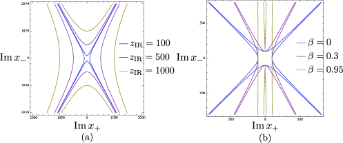
Figure 2: (a) $z_{\rm IR}^{2}=f_{u_{\pm}}({\rm Im}\,x_{+},{\rm Im}\,x_{-};0.3)$ with $z_{\rm IR}=100,500,1000$.
(b) $100^{2}=f_{u_{\pm}}({\rm Im}\,x_{+},{\rm Im}\,x_{-};\beta)$ with $\beta=0,0.3,0.95$.

The hyperbolae (3.5) and (3.9) are shown in Fig. 2. At fixed $\beta$, the hyperbolae escape to spatial infinity, i.e., in the $(x_{+},x_{-})$-plane, as $z_{\rm IR}\to\infty$, see Fig. 2 a. At fixed $z_{\rm IR}$, the angle between the asymptotes of the hyperbolae tends to zero as $\beta\to 1$, see Fig. 2 b.

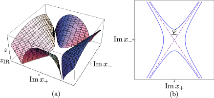
Figure 3: (a) The minimal surface determined by Eqs. (3.4) and (3.8).
(b) The behavior of the surface at fixed $z_{\rm IR}(\geq R^{2}/\alpha)$.

To further clarify the IR behavior of the minimal surface, we show in Fig. 3 a the plot of Eqs. (3.4) and (3.8). The surface blows up and escapes to spatial infinity when $z$ becomes larger. In Fig. 3 b, we show again the hyperbolae defined in Eqs. (3.5) and (3.9), together with their asymptotes. The physical scattering angle $\varphi$ in the $u$-channel is given by

$$\tan{\varphi\over 2}=\sqrt{t\over s}={1-\beta\over 1+\beta}\,,$$ (3.10)

and so it is equal to the angle formed by the asymptotes. Comparison of Fig. 3 b with Fig. 2 b then shows clearly that the scattering angle goes to zero when $\beta\to 1$, that is, in the Regge limit.

In principle, the momentum space formulation of the minimal surface problem considered by Alday and Maldacena can be traded for a coordinate space formulation, with the more complicated boundary discussed above. This is closer in spirit to the variational problem encountered in the eikonal approach, although the boundary in the two cases are living in spaces with different signature, and still on opposite ends of AdS.

3.2 The UV boundary: analytic continuation to Euclidean AdS

The minimal surface solution (2.6) lives in the complexified anti-de Sitter space. If we now perform the following analytic continuation of the world-sheet coordinates,

$$u_{\pm}=iw_{\pm}\,,$$

the coordinates $x_{\pm}$ become real for real $w_{\pm}$. Since $x_{0}$ is still complex, we perform additionally the Wick rotation $x_{4}=ix_{0}$. We then obtain a new minimal surface, given by

$$x_{+} ={R^{2}\over 2\alpha}\bigl{[}(1+\beta)w_{-}+(1-\beta)\cos w_{+}\sin w_{-}\bigr{]}\,,$$ (3.11a)

$$x_{-} =-{R^{2}\over 2\alpha}\bigl{[}(1-\beta)w_{+}+(1+\beta)\sin w_{+}\cos w_{-}\bigr{]}\,,$$ (3.11b)

$$x_{3} =0\,,$$ (3.11c)

$$x_{4} =-{R^{2}\over 2\alpha}\sqrt{1+\beta^{2}}\sin w_{+}\sin w_{-}\,,$$ (3.11d)

$$z ={R^{2}\over 2\alpha}\bigl{[}(1+\beta)\cos w_{+}+(1-\beta)\cos w_{-}\bigr{]}\,,$$ (3.11e)

in the real Euclidean anti-de Sitter space.

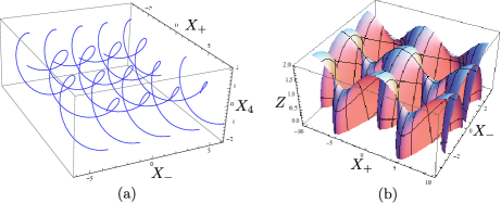
Figure 4: (a) The multiple helices as the UV boundary of Eqs. (3.11) at $z=0$ with $\beta=0.6$.
(b) The minimal surface (3.11) with $\beta=0.6$.

Eq. (3.11e) implies that the minimal surface reaches the UV boundary $z=0$, where it describes a multiple helices configuration (see Fig. 4 a). The axes in Fig. 4 correspond to the coordinates $X_{\pm},X_{4}$ and $Z$, defined by the rescaling $X_{\pm,4}=(2\alpha/R^{2})x_{\pm,4}$ and $Z=(2\alpha/R^{2})z$. The minimal surface (3.11) is depicted in Fig. 4 b. This construction provides a Euclidean formulation of the Alday-Maldacena minimal surface, with boundaries in the UV region, which can be directly compared with the minimal surface problem relevant to the eikonal approach.

A comment is in order here. In Refs. [26, 27], a family of classical string solutions in $AdS_{3}\times S^{3}$ was discussed in terms of the Pohlmeyer reduction of the string sigma model. Ref. [27] obtained a space-like surface in $AdS_{3}$ with conformal complex world-sheet coordinates and embedded it into $AdS_{5}$, so that the Alday-Maldacena type solution was reproduced. Then, by Wick rotation of the world-sheet time coordinate, Ref. [27] found time-like surfaces in $AdS_{3}$, one of which had helicoid geometry. This surface is similar to the one with the double helix boundary that we obtain in the limit $\beta\to 1$, discussed below; however, our Wick rotation and analytic continuations are different from those of Refs. [26, 27].

3.3 The forward Regge limit of the UV boundary

We consider now the forward Regge limit,

$$-s\to\infty,\quad-t\ {\rm fixed},$$ (3.12)

of the solution (3.11). In this limit the Mandelstam variable $u$ goes to $+\infty$, because of the relation $s+t+u=0$. Using the relation (2.5) between the parameters $\alpha,\beta$ of the minimal surface and the Mandelstam variables $s,t$, the limit (3.12) is seen to correspond to $\beta=1$. Since in this limit the scattering angle vanishes, $\varphi=0$, we are dealing here with forward Regge scattering.

In the forward Regge limit, the minimal surface (3.11) in Euclidean space is reduced to

$$x_{+}={R^{2}\over\alpha}w_{-}\,,\quad x_{-}=-{R^{2}\over\alpha}\sin w_{+}\cos w_{-}\,,$$ (3.13)

$$x_{4}=-{R^{2}\over\sqrt{2}\alpha}\sin w_{+}\sin w_{-}\,,\quad z={R^{2}\over\alpha}\cos w_{+}\,,$$

and $x_{3}=0$. At the UV boundary $z=0$, this surface describes a double helix,

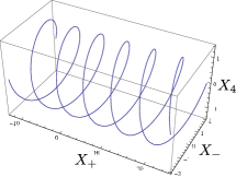
Figure 5: The double helix forming the UV boundary in the forward Regge limit.

$$x_{+}={R^{2}\over\alpha}w_{-}\,,\quad x_{-}=\pm{R^{2}\over\alpha}\cos w_{-}\,,\quad x_{4}=\pm{R^{2}\over\sqrt{2}\alpha}\sin w_{-}\,.$$ (3.14)

The double helix (3.14), depicted in Fig. 5, is reminiscent of the boundary of the minimal surface that was used in Ref. [8] in the computation of the quark-quark scattering amplitude in the eikonal approach. We shall comment on this in the following subsection.

3.4 Relation with the minimal surface for quark-quark scattering in the eikonal approach

In the previous subsection, we have obtained the double helix (3.14) (see Fig. 5) as the boundary of the Euclidean minimal surface (3.13), which appears in the forward Regge limit for gluon-gluon scattering. The boundary of this surface lies on the UV boundary of (Euclidean) anti-de Sitter space. On the other hand, the double helix appears in the context of quark-quark scattering in the eikonal approximation [7, 8, 9], as the IR cutoff of a truncated “generalized helicoid”. Indeed, as we have recalled, the minimal surface relevant to quark-quark scattering, defined by the straight line boundaries (2.18), was studied in Ref. [8] by making the “generalized helicoid” ansätz (2.21). When truncating the surface in order to regularize its area, as in Eq. (2.22), the double helix appears in the projection of the surface on the UV boundary.

Is there a relation between the minimal surfaces used in the Alday-Maldacena approach and in the eikonal approach?

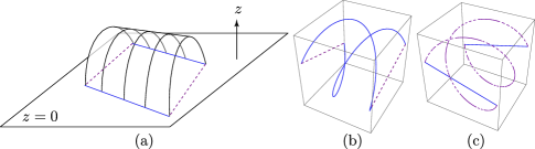
Figure 6: (a) The minimal surface with parallel line segments as the boundary.
(b), (c) The UV boundary and cutoff in the $(x_{+},x_{-},x_{4})$ space at $z=0$.

One can intuitively represent the situation as in Fig. 6. Let us imagine first the minimal surface with two parallel straight-line segments as the UV boundary at $z=0$ in (Euclidean) anti-de Sitter space (Fig. 6 a). This corresponds to the well-known configuration of two parallel Wilson lines used for the computation of the quark-quark potential. The solid line segments in Fig. 6 a describe the boundaries of the minimal surface at $z=0$, while the dotted lines are defined by the IR cutoff imposed on the surface. Twisting the dotted line segments in the $(x_{+},x_{-},x_{4})$ space, we obtain the double helix (Fig. 6 b). This is exactly the geometry of Eqs. (3.14), that is obtained in the forward Regge limit of gluon-gluon scattering in the Alday-Maldacena approach. On the other hand, by twisting the solid line segments in Fig. 6 a, we obtain Fig. 6 c, in which the dotted line segments become the double helix. This is the configuration that is desired in computing the quark-quark scattering amplitude in the eikonal approach. The solid lines describe the trajectories of quarks and the dotted lines are determined by the IR cutoff.

The full answer to the question raised above requires the exact analytic determination of the minimal surface having the boundary configuration of Fig. 6 c, relevant to quark-quark scattering, which could then be compared to the minimal surface found in Ref. [2] for gluon-gluon scattering. However, the exact solution to this problem has not been found yet. Nevertheless, as we will see further on in Section 5, new insights can be obtained by performing a convenient conformal transformation on the minimal surface, and by critically reconsidering the study of the “generalized helicoid” ansätz (2.21).

4 Regge behavior of scattering amplitudes in the
Alday-Maldacena approach

In this Section we discuss the behavior of the gluon-gluon scattering amplitude (2.7), and of the quark-quark scattering amplitude of Ref. [6], in the Regge limit $-s\to\infty$, $t$ fixed (see also Ref. [20]), both in the momentum representation and in the impact-parameter representation.

4.1 Momentum representation

In order to display the Regge behavior of the four-gluon scattering amplitude Eq. (2.7), it is convenient to expand the divergent contributions (2.8) with respect to $\epsilon$. One then obtains

$$iS_{\rm div}(p)=-{1\over\epsilon^{2}}{\sqrt{\lambda}\over 2\pi}+{1\over\epsilon}{\sqrt{\lambda}\over 4\pi}\biggl{(}\log{-p\over\mu^{2}}-1+\log 2\biggr{)}-{f(\lambda)\over 16}\biggl{(}\log{-p\over\mu^{2}}\biggr{)}^{2}+{g(\lambda)\over 8}\log{-p\over\mu^{2}}+{\cal O}(\epsilon)\,,$$ (4.1)

where $p=s,t$, and where we have denoted

$$f(\lambda)={\sqrt{\lambda}\over\pi}\,,\quad g(\lambda)={\sqrt{\lambda}\over\pi}(1-\log 2)\,.$$ (4.2)

The meaning of $f(\lambda)$ and $g(\lambda)$ becomes clear if we rewrite Eq. (4.1) in terms of a new IR cutoff $m$, defined as

$${1\over\epsilon}\equiv\log{m\over\mu}\,.$$ (4.3)

Neglecting terms which do not depend on $p$, we obtain

$$iS_{\rm div}(p)=-{f(\lambda)\over 16}\biggl{(}\log{-p\over m^{2}}\biggr{)}^{2}+{g(\lambda)\over 8}\log{-p\over m^{2}}+(p\hbox{-independent terms})\,,$$ (4.4)

with $f(\lambda)$ appearing in front of the leading IR-divergent term proportional to $(\log m)^{2}$, and $g(\lambda)$ appearing in front of the subleading ($\log m$) divergence.

It is important to note that $f(\lambda)$ appears in the expression of the cusp anomalous dimension $\Gamma_{\rm cusp}(\gamma)$, which represents the contribution of a cusp of boost parameter $\gamma$ to the vacuum expectation value of a Wilson loop in the fundamental representation. For large $|\gamma|$, one has indeed $\Gamma_{\rm cusp}(\gamma)\simeq-\bigl{(}f(\lambda)/4\bigr{)}|\gamma|$. The cusp anomalous dimension [28, 29] is relevant also for the calculation of the anomalous dimension $\gamma_{S}$ of twist-two operators of large spin $S$, $\gamma_{S}\simeq f(\lambda)\log S$ (see, e.g., Ref. [30] and references therein).

Using the expansion (4.1) and the definitions (4.2) and (4.3), the expression of the amplitude (2.7) simplifies

$${\cal A}^{\rm gluon}(s,t) =C_{\epsilon}\biggl{(}{-s\over m^{2}}\biggr{)}^{-{f(\lambda)\over 4}\log{-t\over m^{2}}+{g(\lambda)\over 4}}\biggl{(}{-t\over m^{2}}\biggr{)}^{g(\lambda)\over 4}\,,$$ (4.5)

$$C_{\epsilon} =\exp\biggl{(}-{\sqrt{\lambda}\over\pi}{1\over\epsilon^{2}}+{\tilde{C}}+{\cal O}(\epsilon)\biggr{)}\,.$$ (4.6)

We note that the terms $\log(-s/\mu)^{2}$ and $\log(-t/\mu)^{2}$ in the finite part of Eq. (2.7) are compensated by corresponding terms of order $\epsilon^{0}$ coming from the expansion (4.1) of $S_{\rm div}$ [20].

It is important to realize that formula (4.5) has precisely the form of a Regge amplitude [20, 21] (in particular, it is Regge-exact in the $s$-channel [21]). Indeed, including for completeness also the Born term factor, which for large $-s$ and fixed $t$ reads

$${\cal A}_{\rm tree}\propto{-s\over-t}\,,$$ (4.7)

the gluon-gluon scattering amplitude is of the form

$${\cal A}(s,t)={\cal A}_{\rm tree}\,{\cal A}^{\rm gluon}(s,t)=\beta(t)\biggl{(}{-s\over m^{2}}\biggr{)}^{\alpha(t)},$$ (4.8)

where $\alpha(t)$ is the Regge trajectory,

$$\alpha(t)=\alpha_{0}(t)+\alpha_{1}\,,$$ (4.9)

$$\alpha_{0}(t)=-{f(\lambda)\over 4}\log{-t\over m^{2}}\,,\quad\alpha_{1}={g(\lambda)\over 4}+1\,,$$

and where $\beta(t)$ is given by

$$\beta(t)\propto C_{\epsilon}\biggl{(}{-t\over m^{2}}\biggr{)}^{{g(\lambda)\over 4}-1}\,,$$ (4.10)

up to a $t$-independent constant. In the large-$N_{c}$ limit, the dominant contribution to the amplitude comes from the trajectory with the quantum numbers of the gluon (see Ref. [21] and references therein), so that $\alpha(t)$ is identified as the gluon Regge trajectory.

In the expression of the amplitude (4.5), one may further distinguish the separately factorized terms in $s$ and $t$ from the non-factorizable one, namely

$${\cal A}^{\rm gluon}(s,t)=C_{\epsilon}{\cal A}_{\rm fact}(s){\cal A}_{\rm fact}(t){\cal A}_{\rm nonfact}(s,t)\,,$$ (4.11)

$${\cal A}_{\rm fact}(p)=\exp\biggl{(}{g(\lambda)\over 4}\log{-p\over m^{2}}\biggr{)}\,,\quad(p=s,t)$$ (4.12)

$${\cal A}_{\rm nonfact}(s,t)=\exp\biggl{(}-{f(\lambda)\over 4}\log{-s\over m^{2}}\log{-t\over m^{2}}\biggr{)}\,.$$ (4.13)

As it is well known, the non-factorizable expression (4.13) characterizes the $t$-dependence of the leading Regge trajectory for “octet” $t$-channel exchange, $\alpha_{0}(t)$ in Eqs. (4.9). This term is independent of the particular choice of the IR cutoff: indeed, a rescaling of the IR cutoff $m\to e^{\kappa}m$ leaves it unchanged. On the other hand, the same rescaling changes the coefficient of the logarithm in Eq. (4.12), $g(\lambda)\to g_{\kappa}(\lambda)=g(\lambda)+2\kappa f(\lambda)$, as well as the constant $C_{\epsilon}\to C_{\epsilon,\kappa}=C_{\epsilon}e^{-\kappa^{2}f(\lambda)}$. This results in the dependence of the factorizable terms of the amplitude (4.8) on the regularization scheme: this is not surprising, given the regularization-scheme dependence of the gluon Regge trajectory. Indeed, a calculation in the radial-cutoff scheme, $i.e.$, limiting the integration of the area of the minimal surface (2.4) to $r>r_{c}$, gives [31]

$${\cal A}_{\rm radial}^{\rm gluon}(s,t)=\exp\biggl{(}-{f(\lambda)\over 4}\log{-s\over\tilde{m}^{2}}\log{-t\over\tilde{m}^{2}}+{\rm const.}\biggr{)}\,,$$ (4.14)

where $\tilde{m}=r_{c}/(2\sqrt{2}\pi)$, corresponding to a gluon Regge trajectory with $\alpha_{1}=1$. It is easy to see that the $s,t$-dependent terms in the two schemes are related by the rescaling $\tilde{m}=m\sqrt{e/2}$ of the IR cutoffs.

The key property expected for a Regge trajectory is to be “universal”, i.e., present in all high-energy channels at fixed momentum transfer for the same exchanged quantum numbers. This leads us to compare the results for gluon-gluon scattering discussed above, especially the Regge trajectory (4.9), with the quark-quark elastic scattering amplitude obtained in Ref. [6], along the lines of the Alday-Maldacena approach. We report here only the final result for the color-independent part of the amplitude (divided by the tree amplitude) obtained in the limit of small quark masses, which reads

$${\cal A}^{\rm quark}=\exp\bigg{[}-{f(\lambda)\over 4}\log{-t\over\tilde{m}^{2}}\left(\log{-s\over m_{1}m_{2}}-2(\log(\sqrt{2}-1)+1)\right)+{\rm const.}\bigg{]}\,,$$ (4.15)

where $\tilde{m}=r_{c}/(2\sqrt{2}\pi)$, with $r_{c}$ the radial cutoff used in the calculation, and $m_{1,2}$ are the quark masses. The result above holds as long as $1\ll-s/(m_{1}m_{2})\ll r_{c}^{-1}$, which implies that one cannot take the large-$s$ limit at fixed cutoff. Nevertheless, the term $\log(-s)\log(-t)$ is not affected by a change of the cutoff, which implies that it is reliably captured by the approximation. On the contrary, this is not true for $\log(-s)$ and $\log(-t)$ terms, which are therefore not completely under control at the present stage. It is immediate to see that also this amplitude is of Regge type, with the same $t$-dependent part for the Regge trajectory as in the gluon-gluon case, as expected from universality.

4.2 Impact-parameter representation

For further comparison with the eikonal approach, we derive now the impact-parameter representation for the gluon-gluon scattering amplitude. The impact-parameter amplitude ${\tilde{\cal A}}^{\rm gluon}({\hat{\chi}},b)$ is obtained by performing the two-dimensional Fourier transform of the amplitude ${\cal A}(s,t)$ with respect to the transverse momentum. Setting $-t=k^{2}$ with $k$ the modulus of the transverse momentum, and including the usual factor $s^{-1}$ in the definition of the impact-parameter amplitude, we obtain at large $-s$ (up to an irrelevant constant)

$${\tilde{\cal A}}^{\rm gluon}({\hat{\chi}},b)=C_{\epsilon}\int{dk\over k}\,J_{0}(kb){\cal A}^{\rm gluon}(s,t=-k^{2})\,,$$ (4.16)

where the hyperbolic angle ${\hat{\chi}}$ is defined as

$${\hat{\chi}}=\log{-s\over m^{2}},$$ (4.17)

as appropriate for a $u$-channel process. Azimuthal invariance has been taken into account to reduce the two-dimensional Fourier transform to a Hankel transform of order 0, involving the ordinary Bessel function $J_{0}(\zeta)$ with $\zeta=kb$.

Inserting the amplitude (4.11) into Eq. (4.16), one obtains

$${\tilde{\cal A}}^{\rm gluon}({\hat{\chi}},b) =C_{\epsilon}\bigl{(}m^{2}b^{2}\bigr{)}^{-{1\over 4}h({\hat{\chi}};\lambda)}e^{{g(\lambda)\over 4}{\hat{\chi}}}K({\hat{\chi}})\,,$$ (4.18)

$$h({\hat{\chi}};\lambda) \equiv-f(\lambda){\hat{\chi}}+g(\lambda)\,,$$

where

$$K({\hat{\chi}})\equiv\int_{0}^{\infty}d\zeta\,\zeta^{{1\over 2}h({\hat{\chi}};\lambda)-1}J_{0}(\zeta)=2^{{h\over 2}-1}{\Gamma\bigl{(}{h\over 4}\bigr{)}\over\Gamma\bigl{(}1-{h\over 4}\bigr{)}}\,.$$ (4.19)

The integral (4.19) is convergent in a limited parametric region for $h({\hat{\chi}};\lambda)$, namely $0<h<3$, which lies away from the physical Minkowski region where ${\hat{\chi}}\gg 1$, that is, $h\ll 0$. This is due to the form of the amplitude (4.13), which for $h({\hat{\chi}};\lambda)$ outside of the above-mentioned domain makes the integrand of Eq. (4.16) too singular at small $k$. We can however reach the physically interesting region by means of analytic continuation of the function $K({\hat{\chi}})$ defined in Eq. (4.19), which in the high-energy Minkowski region where ${\hat{\chi}}\gg 1$ becomes

$$K({\hat{\chi}})\approx{1\over e}\bigg{(}{2e\over-h}\bigg{)}^{-{h\over 2}+1}\exp\bigg{[}i\pi\bigg{(}{1\over 2}-{h\over 4}\bigg{)}\bigg{]}\,,$$ (4.20)

where we have made use of Stirling’s formula, $\Gamma(z)\sim\sqrt{2\pi}e^{-z}z^{z-{1\over 2}}$ (for $|z|\to\infty$). Since $h\approx-f(\lambda){\hat{\chi}}$ for ${\hat{\chi}}\gg 1$, in the Minkowski region, we may write the following expansion in energy

$$\log K({\hat{\chi}})=-{f(\lambda)\over 2}{\hat{\chi}}\bigg{(}\log{\hat{\chi}}+\log{f(\lambda)\over 2e}-i{\pi\over 2}\bigg{)}+\bigg{(}{g(\lambda)\over 2}-1\bigg{)}\log{\hat{\chi}}+\cdots\,,$$ (4.21)

where the terms behaving at most as a constant are neglected.

Taking into account the expansion (4.21), the resulting impact-parameter amplitude (4.18) can then be rewritten at high energy and in log form as the expansion

$$-\log{\tilde{\cal A}}^{\rm gluon}({\hat{\chi}},b) =-{f(\lambda)\over 2}{\hat{\chi}}\log{mb}+{f(\lambda)\over 2}{\hat{\chi}}\log{\hat{\chi}}+{\hat{\chi}}\biggl{[}{f(\lambda)\over 2}\biggl{(}\log{f(\lambda)\over 2e}-i{\pi\over 2}\biggr{)}-{g(\lambda)\over 4}\biggr{]}$$ (4.22)

$$\quad+\log{\hat{\chi}}\biggl{(}1-{g(\lambda)\over 2}\biggr{)}+{g(\lambda)\over 2}\log{mb}+\cdots\,,$$

where the overall sign has been chosen for further comparison with the minimal area obtained from the eikonal approach in the following section.

The result (4.22) calls for comments:

• The expansion (4.22) reflects the fact that the amplitude (4.18) is the product of a non-factorizable function of the two kinematic variables, ${\hat{\chi}}$ and $b$, times a factorizable term, namely

  $${\tilde{\cal A}}^{\rm gluon}({\hat{\chi}},b)=C_{\epsilon}(m^{2}b^{2})^{{1\over 4}f(\lambda){\hat{\chi}}}F({\hat{\chi}})B(b)\,,$$ (4.23)

  where the factorizable sector $F({\hat{\chi}})B(b)$ is given by

  $$F({\hat{\chi}})=e^{{1\over 4}g(\lambda){\hat{\chi}}}K({\hat{\chi}})\,,\quad B(b)=(m^{2}b^{2})^{-{1\over 4}g(\lambda)}\,.$$ (4.24)

  The first (non-factorizable) term in (4.22) is the origin of the non-factorizable term in Eq. (4.13), and thus of the $t$-dependent part of the Regge trajectory. The role of the second ($s$-dependent factorizable) term is more subtle, and it is better understood when going back from impact-parameter to momentum space. When taking the inverse Fourier transform, the non-factorizable $b$-dependent term gives rise to a factor $\exp[(f(\lambda)/2){\hat{\chi}}\log{\hat{\chi}}]\sim(\log(-s))^{\log(-s)}$, which is not of Regge type and would be the leading dependence on energy, but which is precisely canceled by the second term. These two terms combine into the expression $-(f(\lambda)/2){\hat{\chi}}\log(mb/{\hat{\chi}})$, which basically encodes the Regge nature of the amplitude. The third and fourth terms yield a factorizable $s$-dependence which modifies the Regge trajectory by a $t$-independent term, and the last term affects the factorizable $t$-dependent part of the amplitude.

• The power of $b$ in Eq. (4.18) is negative in the convergence region where $0<h({\hat{\chi}};\lambda)<3$, while it is positive in the Regge domain $-h({\hat{\chi}};\lambda)=f(\lambda){\hat{\chi}}-g(\lambda)\gg 0$. This is the counterpart in impact-parameter space of the divergence at small values of $k$ in the Fourier transform (4.16). Hence an analytic continuation is required to obtain the impact-parameter amplitude in the interesting high-energy region.

• The non-factorizable sector in Eq. (4.23) depends only on the cusp anomalous dimension at high energy, namely

  $$\Gamma_{\rm cusp}({\hat{\chi}})\to-{f(\lambda)\over 4}{\hat{\chi}}=-{\sqrt{\lambda}\over 4\pi}{\hat{\chi}}\quad{\rm for}\ {\hat{\chi}}\gg 1\,.$$ (4.25)

  It is thus interesting to note that the expression (4.22) can be rewritten as

  $$-\log{\tilde{\cal A}}^{\rm gluon}({\hat{\chi}},b)\approx 2{\Gamma_{\rm cusp}({\hat{\chi}})}\ \log{mb\over{\hat{\chi}}}+\cdots\,,$$ (4.26)

  where we have neglected terms which are subleading in energy, and where we have used the known behavior (4.25) of the cusp anomaly for a fundamental Wilson loop in the large-${\hat{\chi}}$ region.

• It is straightforward to obtain the impact-parameter representation for the quark-quark scattering amplitude of Ref. [6], Eq. (4.15), which can be written as

  $$-\log{\tilde{\cal A}}^{\rm quark}({\tilde{\chi}},b)\approx 2{\Gamma_{\rm cusp}({\tilde{\chi}})}\ \log{\tilde{m}b\over{\tilde{\chi}}}+\cdots\,,$$ (4.27)

  where now ${\tilde{\chi}}=\log(-s/(m_{1}m_{2}))$ is the hyperbolic angle between the classical trajectories of the quarks at high energy, and the dots stand for ${\cal O}(\tilde{\chi})$ terms.

5 Quark-quark scattering amplitude in the eikonal approach

In this section we discuss the minimal surface problem relevant to quark-quark scattering in the eikonal approach, both from a general point of view, and exploiting the “generalized helicoid” ansätz (2.21).

5.1 General features of the minimal surface

On general grounds, the area $A^{\rm quark}_{\rm min}$ of the surface minimizing the functional (2.19) has to take the form

$$A^{\rm quark}_{\rm min}(\theta,b,T)=\Phi_{E}(b/T,\theta)+\Psi_{E}(\theta)\,,$$ (5.1)

where the splitting between a $b$-dependent function $\Phi$ and a $b$-independent one $\Psi$ is made for future convenience. This is a consequence of conformal invariance together with the fact that the IR cutoff $T$ is the only length scale other than $b$ that can appear, once that UV divergencies have been removed. In particular, as we will see below, the separation between the $\Phi$ and $\Psi$ functions amounts to the product of non-factorizable and factorizable contributions to the (Euclidean) impact-parameter amplitude. For future utility, we define the analytic continuation of (5.1) to Minkowski space as

$$A^{{\rm quark},\,s}_{{\rm min},\,M}(\chi,b,T)=A^{{\rm quark}}_{\rm min}(-i\chi,b,iT)\,.$$ (5.2)

This quantity enters the $s$-channel quark-quark scattering amplitude which, in the minimal surface approximation of the AdS/CFT correspondence, is given in impact-parameter space by $\tilde{\cal A}^{{\rm quark},\,s}(\chi,b,T)\equiv\tilde{\cal A}_{E}^{{\rm quark}}(-i\chi,b,iT)=\exp\bigl{[}-A^{{\rm quark},\,s}_{{\rm min},\,M}(\chi,b,T)\bigr{]}$, see Eqs. (2.11) and (2.17). Note that we used the superscript $s$ in the notations in order to specify the physical channel $s\gg 0$ that we consider in Minkowski space.

Further insight on the structure of $A^{\rm quark}_{\rm min}$ can be obtained by performing a particular conformal transformation in Euclidean $AdS_{5}$ space, namely the inversion of coordinates. Such a transformation leaves the area of the surface invariant up to a function of the coupling $\lambda$ only [32], which is not relevant for our purposes. We can therefore investigate the quark-quark scattering amplitude by studying the new minimal surface problem in the inverted coordinates.

Under the transformation of the target space coordinates $(x_{1},x_{2},x_{3},x_{4},z)$ defined by

$$x_{\mu}\to x^{\prime}_{\mu}={x_{\mu}\over|x_{\mu}|^{2}+z^{2}}\,,\quad z\to z^{\prime}={z\over|x_{\mu}|^{2}+z^{2}}\,,$$ (5.3)

the Euclidean $AdS_{5}$ metric is invariant, while the two straight lines $L_{1,2}$, (2.18), which define the boundary condition at $z=0$ in the original coordinates (see Fig. 1), are mapped into two circles $C_{1,2}$, which define the boundary at $z^{\prime}=0$ in the new coordinates:

$$C_{1}:\biggl{(}-{\sin(\theta/2)\over b}\sin\xi,-{1\over b}(1+\cos\xi),0,{\cos(\theta/2)\over b}\sin\xi\biggr{)}\,,$$ (5.4)

$$C_{2}:\biggl{(}{\sin(\theta/2)\over b}\sin\xi,{1\over b}(1+\cos\xi),0,{\cos(\theta/2)\over b}\sin\xi\biggr{)}\,,$$

where

$$\sin\xi={b\tau\over\tau^{2}+b^{2}/4}\,,\quad\cos\xi={-\tau^{2}+b^{2}/4\over\tau^{2}+b^{2}/4}\,.$$ (5.5)

Also in this case, we consider the variational problem for $\tau\in[-\infty,\infty]$, i.e., for two complete circles, and we regularize the area by limiting the integration to $\tau\in[-T,T]$.

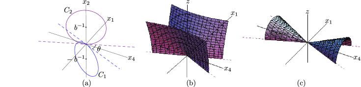
Figure 7: (a) The two circles forming the UV boundary in the inverted coordinates.
(b) The two cusps with angle $\pi-\theta$ around the origin.
(c) The two cusps with angle $\theta$ around the origin.

The two circles $C_{1}$ and $C_{2}$ are centered at $\mp b^{-1}$ in the $x_{2}$-direction, respectively, and have radius $b^{-1}$ (see Fig. 7 a), so that they touch at the origin. More precisely, the regions of the two straight lines corresponding to $-T\leq\tau\leq T$ are mapped into the regions of the circles corresponding to $\xi$ in the range

$$-\pi+\xi_{c}\leq\xi\leq\pi-\xi_{c}\,,\quad 0\leq\xi_{c}\equiv\arcsin{bT\over T^{2}+b^{2}/4}\leq{\pi\over 2}\,,$$ (5.6)

with $\xi_{c}$ approximately equal to $\xi_{c}\sim b/T$ for large $T$. The regions $\tau\leq-T$ and $T\leq\tau$ of the straight lines $L_{1}$ and $L_{2}$ are mapped into two arcs of the circles $C_{1}$ and $C_{2}$, of opening angle $2\xi_{c}$. These arcs have a contact point at the origin, which corresponds to the points at infinity $\tau=\pm\infty$ of the lines $L_{1}$ and $L_{2}$. Around the contact point, where the arcs can be approximated by their tangents, one sees clearly the appearance of two crossing straight lines, which imply therefore the presence of a cusp-like region in the minimal surface (see Fig. 7 b,c).

Indeed, two crossing lines give rise to two pairs of equal angles, namely $\theta$ and $\pi-\theta$. Since the boundaries correspond to fundamental Wilson lines, they have a definite orientation, and so only one pair of angles can contribute. For quark-quark scattering “at angle $\theta$”, the relevant minimal surface is defined in the original coordinates by a boundary formed by the two lines (2.18), and so it is the pair of angles $\pi-\theta$ which gives a cusp contribution to the corresponding minimal surface in the inverted coordinates (see Fig. 7 b). In order to obtain the minimal surface for quark-antiquark scattering “at angle $\theta$”, we have to reverse the orientation of one of the boundaries, as in (2.20), and so in this case it is the pair of angles $\theta$ which gives a cusp contribution (see Fig. 7 c). Of course, this corresponds to quark-quark scattering “at angle $\pi-\theta$”, as repeatedly pointed out.

The appearance of these cusps allows to improve the general expression (5.1) for the regularized area. For this sake, it is convenient to work with the Legendre transform prescription of Ref. [25], in order to get rid of linear UV divergences. It is also convenient to work with the minimal surface obtained in the new, inverted coordinates, which as we have explained above gives the same result for the area up to an irrelevant constant. Let us split the IR-regularized, UV-subtracted area functional evaluated on the minimal surface in the inverted coordinates, which we denote with $A^{\rm quark}_{\rm min}$ by introducing an intermediate time scale $\rho$:

$$A^{\rm quark}_{\rm min}(\theta,b,T) =A^{\rm quark}_{\rm fin}(\theta,b,\rho)+A^{\rm quark}_{\rm div}(\theta,b,T,\rho)\,,$$ (5.7)

$$A^{\rm quark}_{\rm fin}(\theta,b,\rho) =\int_{-\rho}^{\rho}d\tau\int_{-b/2}^{b/2}d\sigma\,{\cal L}\,,$$ (5.8)

$$A^{\rm quark}_{\rm div}(\theta,b,T,\rho) =\biggl{(}\int_{-T}^{-\rho}+\int_{\rho}^{T}\biggr{)}d\tau\int_{-b/2}^{b/2}d\sigma\,{\cal L}\,,$$ (5.9)

where for the sake of simplicity we did not write explicitly the Legendre transform prescription terms. It is well-known that when the cut-off $T\to\infty$, the cusps of the new geometrical boundary defined in (5.4) (see also Fig. 7) provide a logarithmic divergence in the area functional (5.7).

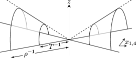
Figure 8: The contribution to $A^{\rm quark}_{\rm div}(\theta,b,T,\rho)$ of the two cusps with angle $\theta$ at the origin.

By introducing an intermediate scale $\rho$, which is kept fixed in the limit $T\to\infty$, we are able to separate the divergent contribution (5.9), which will be dominated by the cusp, from a regular, finite part (5.8), see e.g. Fig. 8. The scale $\rho$ is chosen to be large with respect to $b$ (and thus, after inversion, $\rho^{-1}$ is small compared to the circle diameter in (5.4)), but it is otherwise arbitrary. Using conformal invariance, and exploiting the known properties of Wilson loop expectation values [24, 25, 33], we have that

$$A^{\rm quark}_{\rm div}(\theta,b,T,\rho)=2\Gamma_{\rm cusp}^{E}(\pi-\theta)\log{\rho\over T}+H(\theta,b/T,\rho/T)\,,$$ (5.10)

where $\Gamma^{E}_{\rm cusp}(\Omega)$ is a known function for Euclidean angle $0<\Omega<\pi$ calculated in Ref. [25], and where $H(\theta,b/T,\rho/T)$ is finite in the limit $T\to\infty$. The factor of 2 is due to the fact that there are two cusp contributions. On the other hand, the term $A^{\rm quark}_{\rm fin}$ must take the form $A^{\rm quark}_{\rm fin}(\theta,b,\rho)=G(\theta,\rho/b)$. All in all, we have therefore

$$A^{\rm quark}_{\rm min}(\theta,b,T)=2\Gamma_{\rm cusp}^{E}(\pi-\theta)\log{\rho\over T}+H(\theta,0,0)+G(\theta,\rho/b)+o(T^{0})\,,$$ (5.11)

where $o(T^{0})$ stands for terms which vanish in the limit $T\to\infty$. As we have already said, the scale $\rho$ is a fixed intermediate scale, allowing to singularize the cusp contribution to the area. Now, since $\rho$ is arbitrary, it should disappear from the right-hand side of Eq. (5.11), and this is possible only if

$$G(\theta,\rho/b)=-2\Gamma_{\rm cusp}^{E}(\pi-\theta)\log{\rho\over b}+{\hat{G}}(\theta)\,.$$ (5.12)

This can be looked at also in a different way. We can take $\rho$ to be not an arbitrary “external” scale, but the one determined by the exact solution of the minimal surface problem, that separates the region where the surface is well approximated by a cusp solution from the rest. For dimensional reasons, it must be of the form $\rho=b\,g(\theta)$, so that Eq. (5.12) again follows.

In conclusion, comparing the minimal area (5.1) with (5.11), we can write

$$\Phi_{E}(b/T,\theta)=2\Gamma_{\rm cusp}^{E}(\pi-\theta)\log{b\over T}+o(T^{0})\,.$$ (5.13)

We notice that Eq. (5.13) contains only the contribution of the region around the contact point of the two circles, which is related by inversion to the region at infinity of the two straight lines. In other words, the $b,T$-dependent term Eq. (5.13) is determined only by the initial and final data of quarks, and this reflects well the link between the eikonal approximation and the dominance of the cusps. The relation between the cusp anomalous dimension and the high-energy behavior of scattering amplitudes is a well-known fact, but it is not evident a priori how this relation would show up in the eikonal approach, where no cusp is present in the initial setting, in the strong-coupling regime. The result Eq. (5.13) thus provides a first nontrivial check for the viability of the eikonal approach.

On the other hand, the function $\Psi_{E}(\theta)$ in Eq. (5.1) remains to be determined, which would require the exact solution of the minimal surface problem, which is not available at the moment. However, it is possible to go further and determine an interesting approximation by using the “generalized helicoid” ansätz (2.21). It amounts to find a refined estimate of the intermediate scale $\rho$, in the “natural” sense discussed after Eq. (5.12), isolating more precisely the (truncated) cusp contribution.

5.2 The “generalized helicoid” ansätz

Let us go back to the regularized area functional (2.22) derived from the area functional (2.19) with “generalized helicoid” ansätz (2.21), discussed in Section 2. Following Ref. [8], we make the change of variables

$$\sigma^{\prime}\equiv\sigma\sqrt{1+\biggl{(}{\theta\tau\over b}\biggr{)}^{2}}\,,\quad z^{\prime}(\tau,\sigma^{\prime})\equiv z(\tau,\sigma(\tau,\sigma^{\prime}))\,,$$ (5.14)

which leads to the following expression for the area functional,

$$A^{\rm quark}_{\pi-\theta,b}={\sqrt{\lambda}\over 2\pi}\int_{-T}^{T}d\tau\int_{-{b\over 2}\sqrt{1+\left({\theta\tau\over b}\right)^{2}}}^{{b\over 2}\sqrt{1+\left({\theta\tau\over b}\right)^{2}}}d\sigma{1\over z^{2}}\sqrt{1+(\partial_{\sigma}z)^{2}+\Biggl{(}\partial_{\tau}z+{\bigl{(}{\theta\tau\over b}\bigr{)}\bigl{(}{\theta\sigma\over b}\bigr{)}\over 1+\bigl{(}{\theta\tau\over b}\bigr{)}^{2}}\,\partial_{\sigma}z\Biggr{)}^{2}}\,,$$ (5.15)

where we have dropped the primes for simplicity. As we have already remarked, the ansätz (2.21) is appropriate for quark-antiquark scattering, as indicated by the subscript $\pi-\theta$.

It can be realized that, written in the form (5.15), the “generalized helicoid” ansätz admits interesting approximate while explicit solutions for both the large and small $|\tau|$ regions.

• Small-$|\tau|$ region, i.e., $\theta|\tau|/b\ll 1$
  In this region the corresponding contribution to the area functional simplifies to

  $$A^{\rm quark}_{\pi-\theta,b}\big{|}_{{\rm small}\,\tau}={\sqrt{\lambda}\over 2\pi}\int_{-\delta{b/\theta}}^{\delta{b/\theta}}d\tau\int_{-b/2}^{b/2}d\sigma{1\over z^{2}}\sqrt{1+(\partial_{\sigma}z)^{2}+(\partial_{\tau}z)^{2}}\,,$$ (5.16)

  where $\delta$ is some small positive number. This functional corresponds to the area functional of a minimal surface with planar boundaries, where the symmetries of the problem allow to write the solution in the form

  $$t=\tau\,,\quad x={\rm constant}\,,\quad y=\sigma\,,\quad z=z(\tau,\sigma)\,.$$ (5.17)

  Moreover, in our case the boundary is made up of two segments of parallel straight lines of length $2\delta{b/\theta}$ at a distance $b$, for which the solution is known [24]. The corresponding (regularized and UV-subtracted) area is

  $$A^{\rm quark}_{\rm min}(\pi-\theta,b,T)\bigr{|}_{{\rm small}\,\tau}\simeq-{\sqrt{\lambda}\over 2\pi}c{2\delta b\over\theta}{1\over b}=-{\sqrt{\lambda}\over 2\pi}{2c\delta\over\theta}\,,$$ (5.18)

  where the constant $c=8\pi^{3}/\Gamma^{4}(1/4)$ is the coefficient in front of the (screened) coulombic potential [24]. One immediately sees that after analytic continuation this contribution is vanishing with energy, both for the quark-quark ($\theta\to\pi+i\chi$) and for the quark-antiquark ($\theta\to-i\chi$) $s$-channel scattering processes, in the limit $\chi\to\infty$.

• Large-$|\tau|$ region, i.e., $\theta|\tau|/b\gg 1$
  Eq. (5.15) is also suitable for an analytic solution in the large $\tau$ region. Neglecting 1 against $\theta\tau/b$, the area functional simplifies to

  $$A^{\rm quark}_{\pi-\theta,b}\bigr{|}_{{\rm large}\,\tau}={\sqrt{\lambda}\over 2\pi}\biggl{(}\int_{-T}^{-\Lambda{b\over\theta}}+\int_{\Lambda{b\over\theta}}^{T}\biggr{)}d\tau\int_{-{\theta|\tau|\over 2}}^{{\theta|\tau|\over 2}}d\sigma{1\over z^{2}}\sqrt{1+(\partial_{\sigma}z)^{2}+\Bigl{(}\partial_{\tau}z+{\sigma\over\tau}\partial_{\sigma}z\Bigr{)}^{2}}\,,$$ (5.19)

  where $\Lambda$ is some large number. Away from the boundary, where $|\sigma/\tau|$ is small, Eq. (5.19) can be further approximated as

  $$A^{\rm quark}_{\pi-\theta,b}\bigr{|}_{{\rm large}\,\tau}={\sqrt{\lambda}\over 2\pi}\biggl{(}\int_{-T}^{-\Lambda{b\over\theta}}+\int_{\Lambda{b\over\theta}}^{T}\biggr{)}d\tau\int_{-{\theta|\tau|\over 2}}^{{\theta|\tau|\over 2}}d\sigma\,{1\over z^{2}}\sqrt{1+(\partial_{\sigma}z)^{2}+\left(\partial_{\tau}z\right)^{2}}\,.$$ (5.20)

  We have again to deal with a minimal surface with planar boundary, which this time consists of two segments of straight lines at an angle $\theta$,

  $$\sigma_{\pm}(\tau)=\pm{\theta\tau\over 2}\,,$$ (5.21)

  with $|\tau|\in[\Lambda b/\theta,T]$. The solution is immediately seen to be made up of two parts, each corresponding to a piece of the solution for a cusp of angle $\theta$ (cf. Fig. 8), and the resulting (regularized and UV-subtracted) area is

  $$A^{\rm quark}_{\rm min}(\pi-\theta,b,T)\bigr{|}_{{\rm large}\,\tau}=2\Gamma_{\rm cusp}^{E}(\theta)\log{\Lambda b\over T\theta}\,.$$ (5.22)

  This result is in agreement with the general form (5.1) for the minimal area, and moreover allows to determine the “natural” choice of a $\theta$-dependent scale $\rho\sim\Lambda b/\theta$, discussed after Eq. (5.12), which separates the near-cusp region from the rest in the inverted coordinates. Indeed, up to the constant $\Lambda$, whose precise value cannot be determined at the present stage, we have that $\rho\propto b/\theta$. The factor $1/\theta$ could not be predicted with the general arguments of the previous subsection: its important role will become clear after analytic continuation to Minkowski space. Let us finally remark that Eq. (5.22) gives also an estimate of the function $\Psi_{E}(\theta)$ in Eq. (5.1):

  $$\Psi_{E}(\theta)\sim 2\Gamma_{\rm cusp}^{E}(\theta)\log{\Lambda\over\theta}\,,$$ (5.23)

  up to the term Eq. (5.18), which as we have explained gives a vanishing contribution after analytic continuation, and up to possible contributions from the intermediate region $\tau\theta/b\in[\delta,\Lambda]$, as well as from the region $\sigma\simeq(\theta/2)\tau$. In a sense, the constant $\Lambda$ stands for our ignorance about the $b,T$-independent term $\Psi_{E}(\theta)$.

We are now ready to perform the analytic continuation. Neglecting subleading contributions, and considering for definiteness the quark-quark $s$-channel, so that the relevant analytic continuation reads

$$\theta\to\pi+i\chi\,,\quad T\to iT\,,$$ (5.24)

with $\chi\sim\log(s/M^{2})$, $s>0$, we obtain

$$A^{{\rm quark},\,s}_{{\rm min},\,M}(\chi,b,T)=2\Gamma_{\rm cusp}(\chi)\log{\Lambda b\over T\chi e^{i\pi}\bigl{(}1+e^{-i{\pi\over 2}}(\pi/\chi)\bigr{)}}=2\Gamma_{\rm cusp}(\chi)\log{b\over T\chi}+{\hat{\Psi}}^{s}_{M}(\chi)\,,$$ (5.25)

where we have used $\Gamma_{\rm cusp}^{E}(\pi+i\chi)=\Gamma_{\rm cusp}(\chi)$ [30]. Taking the limit $\chi\to\infty$, we obtain for the $b,T$-dependent term and for the leading $\chi$-dependence

$$A^{{\rm quark},\,s}_{{\rm min},\,M}(\chi,b,T)=-{f(\lambda)\over 2}\chi\log{b\over T\chi}+{\cal O}(\chi)\,,$$ (5.26)

where we have used Eq. (4.25), which also implies that the auxiliary function ${\hat{\Psi}}^{s}_{M}(\chi)={\cal O}(\chi)$ in (5.26).

The $u$-channel quark-quark amplitude,

$${\tilde{\cal A}}^{{\rm quark},\,u}(\chi,b,T)\equiv\exp\bigl{[}-A^{{\rm quark},\,u}_{{\rm min},\,M}(\chi,b,T)\bigr{]}\quad\bigl{(}=\tilde{\cal A}^{{\rm quark}}_{E}(\pi+i\chi,b,iT)\bigr{)}\,,$$ (5.27)

that we shall use in the next subsection for the comparison with the results of the Alday-Maldacena approach, is obtained by means of the crossing-symmetry relations (2.12), $i.e.$, through the analytic continuation²³

$$\theta\to-i\chi\,,\quad T\to iT\,,$$ (5.28)

with $\chi\sim\log(-s/M^{2})$, $u\sim-s>0$, which yields

$$A^{{\rm quark},\,u}_{{\rm min},\,M}(\chi,b,T)=2\Gamma_{\rm cusp}(i\pi-\chi)\log{\Lambda b\over T\chi}=2\Gamma_{\rm cusp}(i\pi-\chi)\log{b\over T\chi}+{\hat{\Psi}}^{u}_{M}(\chi)\,.$$ (5.29)

Although the exact value of $\Gamma_{\rm cusp}(i\pi-\chi)$ is not yet known, we expect that its large-$\chi$ behavior coincides with that of $\Gamma_{\rm cusp}(\chi)$ (this is actually the case in perturbation theory [28, 29]), so that in the limit $\chi\to\infty$ the leading term reads

$$A^{{\rm quark},\,u}_{{\rm min},\,M}(\chi,b,T)=-{f(\lambda)\over 2}\chi\log{b\over T\chi}+{\cal O}(\chi)\,,$$ (5.30)

which also implies that the auxiliary function in the $u$-channel verifies ${\hat{\Psi}}^{u}_{M}={\cal O}(\chi)$.

Our result (5.30) calls for a comment related to the initial approach of Ref. [8]. In Ref. [8], the functionals (2.22) and (5.15) were the starting point for an approximate evaluation of the area of the minimal surface. In particular, the aim of the authors was to determine the $T$-independent, IR-finite contribution to the area. To this extent, neglecting the non-diagonal terms in $\partial_{\tau}z$, $\partial_{\sigma}z$ in Eq. (5.15), they performed the angular part only of the analytic continuation, i.e., $\theta\to-i\chi$ (see Eqs. (31)–(34) in Ref. [8]). The $T$-independent part of the resulting functional turned out to be the area $A_{\rm ellipse}$ of a simpler minimal surface, living in Euclidean $AdS_{5}$, and having as boundary a half-ellipse of width $b/\chi$ and height $b$. Finally, the approximate evaluation of $A_{\rm ellipse}$ led to the following result:

$$A_{\rm ellipse}=-2\Gamma_{\rm cusp}^{E}\Bigl{(}{\pi\over 2}\Bigr{)}\log{M_{B}b\over\chi}-{\sqrt{\lambda}\over 2\pi}{c\pi\over 4}\chi\,,$$ (5.31)

where $\Gamma_{\rm cusp}^{E}(\pi/2)$ is the Euclidean cusp anomaly calculated in Refs. [25, 30] and $c$ is the same constant as that in Eq. (5.18). The scale $M_{B}^{-1}$ is the inverse mass of the $W$-bosons playing the role of “Euclidean quarks”, see Section 2, and corresponds to the position of the D3-brane which acts as UV cutoff.

Our present study gives a different and improved answer to the problem initiated by Ref. [8], as shown by comparing (5.30) and (5.31). In this paper we have gone beyond the approximations made in Ref. [8], whose results suffer from the limited knowledge on minimal surface solutions for scattering amplitudes available at that time, in particular regarding the geometry relevant for quark-quark scattering in the eikonal approach. The key point here are the non-diagonal terms in the area functional (5.15), which cannot be neglected in the region considered in Ref. [8]. Though functionally similar to (5.30) (by the interchange of $\Gamma_{\rm cusp}^{E}(\pi/2)$ with $\Gamma_{\rm cusp}(i\pi-\chi)$), the expression (5.31) does not contribute a non-factorizable factor to the amplitude. Moreover, the expression (5.31) shows the appearance in the logarithmic term of the UV-cutoff $M_{B}$. As discussed above, $M_{B}$ should drop from the area when UV divergencies have been removed.

5.3 Eikonal vs. Alday-Maldacena approach

Let us finally compare our results for quark-quark scattering, obtained in the eikonal approach, with the ones obtained for gluon-gluon scattering using the Alday-Maldacena solution. Since we are interested in the high-energy Regge behavior of the amplitude, this is a sensible comparison to be made, due to the universality property discussed in Section 4.

For convenience, we rewrite here the $u$-channel quark-quark scattering amplitude obtained with the eikonal approach (see Eqs. (5.27) and (5.30)),

$$-\log{\tilde{\cal A}}^{{\rm quark},\,u}_{\rm eikonal}(\chi,b,T)=-{f(\lambda)\over 2}\chi\log{b\over T\chi}+{\cal O}(\chi)=-{f(\lambda)\over 2}{\hat{\chi}}\log{b\over T{\hat{\chi}}}+{\cal O}({\hat{\chi}})\,,$$ (5.32)

where we used $\chi={\hat{\chi}}+\log(m^{2}/M^{2})$, see Eqs. (2.13) and (4.17), and also the gluon-gluon scattering amplitude in impact-parameter space and in the Regge limit obtained with the Alday-Maldacena approach, Eq. (4.22),

$$-\log{\tilde{\cal A}_{\rm AM}^{{\rm gluon}}}({\hat{\chi}},b,m)=-{f(\lambda)\over 2}{\hat{\chi}}\log{mb\over{\hat{\chi}}}+{\hat{\chi}}\biggl{[}{f(\lambda)\over 2}\biggl{(}\log{f(\lambda)\over 2e}-i{\pi\over 2}\biggr{)}-{g(\lambda)\over 4}\biggr{]}+\cdots\,,$$ (5.33)

where we have made explicit the dependence of the amplitude on the IR regulator $m$, and we have specified which approach has been used with appropriate subscripts.

Examining the expression for the quark amplitude (5.32) following the order in the expansion of the exact expression (5.33) for the gluon one, the following consequences can be drawn:

• First term
  The first term exactly coincides with the leading term (4.26) obtained in the case of gluon-gluon scattering from the Alday-Maldacena solution, up to a rescaling $T\to m^{-1}$, i.e. up to a shift

  $$-{f(\lambda)\over 2}{\hat{\chi}}\log{mT}={\cal O}({\hat{\chi}})$$

  which plays a role at next to leading order only. Looking back to the discussion of the exact gluon-gluon amplitude (4.5), we noticed that the first term in its impact-parameter representation Eq. (4.22), coinciding with (4.26) at high energy, was at the origin of the Regge nature of the amplitude, and of the $t$-dependent part of the Regge trajectory (4.9). This implies that the quark-quark (and also quark-antiquark) scattering amplitude is of Regge type, and that the $t$-dependent part of the Regge trajectory is indeed the same obtained in the Alday-Maldacena approach.
  Hence the main conclusion is that the same Regge factor $(-s)^{-(f(\lambda)/4)\log(-t)}$ appears in the $(s,t)$-representation of both amplitudes. This corresponds to the fact that both amplitudes in impact-parameter space contain the same term, i.e., $2\Gamma_{\rm cusp}({\hat{\chi}})\log[{\rm(mass)}\cdot b/{\hat{\chi}}]$. In particular, we notice that the $t$-dependent part of the Regge trajectory comes entirely from the non-factorizable term $2\Gamma_{\rm cusp}({\hat{\chi}})\log[{\rm(mass)}\cdot b]$, which has been obtained through the general considerations of Section 5.1 (see Eq. (5.13)). This is therefore a robust result, independent of the approximations performed in Section 5.2. It is also interesting to note that the leading term of order ${\hat{\chi}}\log{\hat{\chi}}$ in the factorized ${\hat{\chi}}$-dependent part appears to be the same, while coming from seemingly different origin in the two cases: in the quark amplitude it comes from a refined evaluation of the cusp contribution, see e.g. (5.23), with the “generalized helicoid” ansätz, while in the gluon case it comes from the Fourier transform factor (4.19) after analytic continuation. As we have already remarked, this term is essential in order to obtain an amplitude of Regge type.

• Second term
  The ${\cal O}({\hat{\chi}})$ term in (5.32) is compatible with Regge behavior. At the present stage we are not able to find a precise evaluation of this term, which could be obtained from the full solution of the minimal surface problem. However, as it has already been shown for the gluon case (see Eqs. (4.8)–(4.10)), it may affect only the factorized part of the amplitude, which depends on the regularization scheme. In particular, the $t$-dependent factorized term of the amplitude is not expected to be universal, but to depend on the species of the scattering particles.

• $f\log f$ term
  The $f\log f$ term in (5.33) may seem puzzling at first, since no term of this kind can be found in the expression for the area of the minimal surface in the eikonal approach. However, its origin becomes evident when one recalls that the radial coordinates $r$ and $z$ used in the two approaches are related as $r=R^{2}/z=\sqrt{\lambda}/z$, so that an appropriate conversion factor has to be used when comparing the IR cutoffs. This is particularly clear if one uses the radial cutoff $r_{c}$, which, as we have discussed above in Section 4, is related to the cutoff $m$ in the dimensional regularization scheme as $m=\tilde{m}\sqrt{2/e}={r_{c}/(2\pi\sqrt{e})}$. In turn, $r_{c}$ can be expressed as $r_{c}=R^{2}/z_{c}=\sqrt{\lambda}/z_{c}$ in terms of the radial coordinate $z$, with $z_{c}\to\infty$ when the IR regularization is removed, which is appropriate for comparing the Alday-Maldacena result with the eikonal approach. Expressing the leading term in Eq. (5.33) in terms of this new cutoff, we see that the $f\log f$ term actually gets cancelled, and we obtain the expression

  $$-\log{\tilde{\cal A}}_{\rm AM}^{\rm gluon}({\hat{\chi}},b,z_{c})=-{f(\lambda)\over 2}\hat{\chi}\log{b\over z_{c}{\hat{\chi}}}-{f(\lambda)\over 2}\hat{\chi}\bigg{(}1-\log\sqrt{2}+i{\pi\over 2}\bigg{)}+\cdots\,.$$ (5.34)

  The cutoff $z_{c}$ can now be identified with $T$, up to numerical factors which affect only the regularization-scheme dependent part of the amplitude. In other words, the shift proportional to $\log{mT}$, discussed above in point i), naturally contains the appropriate “counterterm” which makes $f\log f$ drop from the complete expression.

• Gluon-gluon scattering
  To conclude this section, we want to briefly discuss how the technique applied above to quark-quark scattering is extended to the case of gluon-gluon scattering. Recall from Section 2 the expressions (2.27) and (2.29) for the “octet” component of the amplitude. Using large-$N_{c}$ factorization and minimal surfaces, we have to leading order in $N_{c}$

  $$\langle{\rm tr}W_{1}^{{\dagger}}{\rm tr}W_{2}^{{\dagger}}{\rm tr}[W_{1}W_{2}]\rangle \sim\langle{\rm tr}W_{1}^{{\dagger}}\rangle\langle{\rm tr}W_{2}^{{\dagger}}\rangle\langle{\rm tr}[W_{1}W_{2}]\rangle$$

  $$\phantom{aaaaaaaaaaaaaaai}\sim N_{c}^{3}\biggl{(}1+e^{-A^{\rm quark}_{\rm min}(\theta,b,T)}\biggr{)}$$ (5.35)

  $$\langle{\rm tr}W_{1}{\rm tr}W_{2}^{{\dagger}}{\rm tr}[W_{1}^{{\dagger}}W_{2}]\rangle \sim\langle{\rm tr}W_{1}\rangle\langle{\rm tr}W_{2}^{{\dagger}}\rangle\langle{\rm tr}[W_{1}^{{\dagger}}W_{2}]\rangle$$

  $$\phantom{aaaaaaaaaaaaaaai}\sim N_{c}^{3}\biggl{(}1+e^{-A^{\rm quark}_{\rm min}(\pi-\theta,b,T)}\biggr{)}$$ (5.36)

  $$\langle|{\rm tr}W_{1}{\rm tr}W_{2}|^{2}\rangle \sim|\langle{\rm tr}W_{1}\rangle\langle{\rm tr}W_{2}\rangle|^{2}\sim N_{c}^{4}\,,$$ (5.37)

  and moreover $Z_{V}\sim{1\over N_{c}^{2}}\langle{\rm tr}W_{i}\rangle\langle{\rm tr}W_{i}^{{\dagger}}\rangle\sim 1$. We therefore conclude that

  $${\cal A}^{gg}_{N_{c}^{2}-1,A}\sim N_{c}^{3}\biggl{(}e^{-A^{\rm quark}_{\rm min}(\theta,b,T)}-e^{-A^{\rm quark}_{\rm min}(\pi-\theta,b,T)}\biggr{)}$$

  $$\mathop{\to}_{\theta\to-i\chi,T\to iT}~{}~{}~{}N_{c}^{3}\biggl{(}{\tilde{\cal A}}^{{\rm quark},\,s}_{\rm eikonal}(\chi,b,T)-{\tilde{\cal A}}^{{\rm quark},\,u}_{\rm eikonal}(\chi,b,T)\biggr{)}\,,$$ (5.38)

  $${\cal A}^{gg}_{N_{c}^{2}-1,S}\sim N_{c}^{3}\biggl{(}e^{-A^{\rm quark}_{\rm min}(\theta,b,T)}+e^{-A^{\rm quark}_{\rm min}(\pi-\theta,b,T)}\biggr{)}$$

  $$\mathop{\to}_{\theta\to-i\chi,T\to iT}~{}~{}~{}N_{c}^{3}\biggl{(}{\tilde{\cal A}}^{{\rm quark},\,s}_{\rm eikonal}(\chi,b,T)+{\tilde{\cal A}}^{{\rm quark},\,u}_{\rm eikonal}(\chi,b,T)\biggr{)}\,.$$ (5.39)

  As already anticipated in the Introduction, the calculation in the gluon-gluon case reduces basically to that of the quark-quark case. Moreover, it is evident from Eqs. (5.38) and (5.39) that the high-energy behavior is the same in the two cases. In particular, together with the expressions (5.26) and (5.30)–(5.32) for the high energy behavior of the quark amplitudes, this result shows that also the “octet” component of the gluon-gluon scattering amplitude is of Regge type, with the same gluon Regge trajectory as in the quark-quark case, and therefore with the same $t$-dependent part of the trajectory found by Alday and Maldacena. As a final remark, we want to stress the fact that universality is shown in a simpler way in the eikonal approach, thanks to the fact that the basic object in the computation of the scattering amplitude is the correlation function of the same Wilson lines, differing only for the representation in which they are taken.

6 Summary, comments and outlook

In this work we have investigated the Regge behavior of high-energy amplitudes in ${\cal N}\!=\!4$ supersymmetric Yang-Mills theory at strong coupling, using the AdS/CFT correspondence in two different ways. For this sake we have analyzed these amplitudes in the dual gravity theory, where they are obtained as the (regularized) area of minimal surfaces in Minkowskian AdS and hyperbolic (or “Euclidean AdS”) backgrounds. We summarize here the main points.

• In order to make easier the comparison with the eikonal approach, the Alday-Maldacena four-gluon amplitude [2], obtained from a minimal surface in Minkowskian AdS, has been put in a Regge form [20, 21], see formulas (4.8) and (4.9), namely

  $${\cal A}(s,t)\equiv\beta(t)\biggl{(}{-s\over m^{2}}\biggr{)}^{\alpha(t)}\propto C_{\epsilon}\biggl{(}{-t\over m^{2}}\biggr{)}^{{g(\lambda)\over 4}-1}\biggl{(}{-s\over m^{2}}\biggr{)}^{\alpha(t)}\ ,$$ (6.1)

  where $m$ is an IR cut-off and $\alpha(t)$ is the Regge trajectory,

  $$\alpha(t)=-{f(\lambda)\over 4}\log{-t\over m^{2}}+{g(\lambda)\over 4}+1\,,$$ (6.2)

  $C_{\epsilon}$ is a regularization-dependent constant, and the functions $f(\lambda)$ and $g(\lambda)$ have been defined in Eqs. (4.2). It is known that the trajectory is identified with the gluon Regge trajectory [21], corresponding to the exchange of gluon quantum numbers between the colliding particles. The same $t$-dependent part of the Regge trajectory is found in the quark-quark elastic scattering calculation of Ref. [6], in accordance with the expected universality of the Regge behavior.
  In order to compare this to the results obtained in the eikonal approach, we have also studied the corresponding impact-parameter representation, where the Regge nature of the amplitude is encoded in the leading factor $(mb/\chi)^{-{f(\lambda)\over 2}\chi}$.

• We have computed the “octet”-exchange component of the quark-quark and quark-antiquark elastic amplitude at high-energy in the impact-parameter representation, by using the eikonal method in hyperbolic space [8]. This amounts to consider the (regularized) minimal surface corresponding to a “generalized helicoid” in hyperbolic space, i.e. the surface bounded by two straight lines at the Euclidean boundary. By performing a conformal transformation, we have shown that the minimal area is dominated by the contribution of two identical cusps, which leads to the same $t$-dependent part $-(f(\lambda)/4)\log(-t/m^{2})$ of the Regge trajectory (6.2), where $f(\lambda)/4$ is the coefficient of the cusp anomalous dimension in Minkowski space (4.25). This shows the compatibility between the two a priori very different approaches, making us confident in the viability of the eikonal method in the physically interesting case of QCD, where the Alday-Maldacena method is not available.

• We have also computed the “octet”-exchange component of the gluon-gluon elastic scattering amplitude in the eikonal approach, which boils down to a linear combination of the corresponding results for quark-quark and quark-antiquark scattering. In this way we have shown universality of the Regge behavior in the framework of the eikonal method, which is obtained in a simpler way than in the Alday-Maldacena approach.

Let us finally propose an outlook on open questions.

The Alday-Maldacena solution (2.6) in the position space is described in terms of complex coordinates, namely the target space is extended to the complexified $AdS_{5}$. We have generated the new minimal surface (3.11) from Eqs. (2.6) by performing the Wick rotation of the time coordinate of $AdS_{5}$, as well as of the two world-sheet coordinates. The resulting surface is embedded into the ordinary Euclidean $AdS_{5}$, and its boundary lies in the UV region ($i.e$, near the boundary $z=0$ of Euclidean $AdS_{5}$), while on the other hand the surface described by the Alday-Maldacena solution has its boundary in the IR region of (Minkowskian) $AdS_{5}$. We have found that the UV boundary of our solution is a set of multiple helices; in particular, in the forward Regge limit, $-s\to\infty$ with $-t$ fixed, the boundary reduces to a double helix. This hints to the existence of a helicoid structure common to the two approaches, which however results in different surfaces in the Euclidean AdS background, in some sense “dual” under interchange of two boundaries of a truncated helicoid, see Fig. 6. Further studies are required in order to fully understand this similarity.

In order to perform the comparison between the two approaches, we have calculated both scattering amplitudes in the same Minkowskian impact parameter $(b,s)$-representation. The amplitudes consist of non-factorizable and factorizable parts with respect to $b$ and $s$. The area of both minimal surfaces contains the same leading non-factorizable term $2\Gamma_{\rm cusp}({\hat{\chi}})\log(mb/{\hat{\chi}})$ with $\hat{\chi}\sim\log s$ (under the rescaling $m\to T^{-1}$, and up to subleading terms), compare (5.32) with (5.33), which leads to the same $t$-dependent part of the Regge trajectory, as we have already remarked. The exact subleading term has not yet been obtained in the eikonal approach, which requires the exact solution of the “generalized helicoid” problem.

An important point concerns the physical relevance of the subleading terms in $\chi$. Such terms are not known in the eikonal approach, due to the lack of an exact solution for the minimal surfface. However, such terms are finally involved in the regularization-scheme dependence, and one may ask what is their physical relevance. Stated differently, would we know more about the physics of scattering amplitudes if we knew those terms exactly? This is an open problem for future investigations.

Acknowledgments

MG and SS are grateful to IPhT, CEA-Saclay for hospitality. MG was supported by MICINN under the CPAN project CSD2007-00042 from the Consolider-Ingenio2010 program, as well as under the grant FPA2009-09638.

References

- [1] J. M. Maldacena, “The large N limit of superconformal field theories and supergravity,” Adv. Theor. Math. Phys. 2 (1998) 231 [Int. J. Theor. Phys. 38 (1999) 1113] [arXiv:hep-th/9711200].
- [2] L. F. Alday and J. M. Maldacena, “Gluon scattering amplitudes at strong coupling,” JHEP 0706 (2007) 064 [arXiv:0705.0303 [hep-th]].
- [3] L. F. Alday and J. Maldacena, “Comments on gluon scattering amplitudes via AdS/CFT,” JHEP 0711 (2007) 068 [arXiv:0710.1060 [hep-th]].
- [4] J. McGreevy and A. Sever, “Quark scattering amplitudes at strong coupling,” JHEP 0802 (2008) 015.
- [5] Z. Komargodski and S. S. Razamat, “Planar quark scattering at strong coupling and universality,” JHEP 0801 (2008) 044 [arXiv:0707.4367 [hep-th]].
- [6] E. Barnes and D. Vaman, “Massive quark scattering at strong coupling from AdS/CFT,” Phys. Rev. D 81 (2010) 126007 [arXiv:0911.0010 [hep-th]].
- [7] R. A. Janik and R. B. Peschanski, “High energy scattering and the AdS/CFT correspondence,” Nucl. Phys. B 565 (2000) 193 [arXiv:hep-th/9907177].
- [8] R. A. Janik and R. B. Peschanski, “Minimal surfaces and Reggeization in the AdS/CFT correspondence,” Nucl. Phys. B 586 (2000) 163 [arXiv:hep-th/0003059].
- [9] R. A. Janik and R. B. Peschanski, “Reggeon exchange from AdS/CFT,” Nucl. Phys. B 625 (2002) 279 [arXiv:hep-th/0110024].
- [10] O. Nachtmann, “Considerations concerning diffraction scattering in quantum chromodynamics,” Annals Phys. 209 (1991) 436.
- [11] H. G. Dosch, E. Ferreira and A. Kramer, “Nonperturbative QCD treatment of high-energy hadron hadron scattering,” Phys. Rev. D 50 (1994) 1992 [arXiv:hep-ph/9405237].
- [12] E. Meggiolaro, “A Remark on the high-energy quark quark scattering and the eikonal approximation,” Phys. Rev. D 53 (1996) 3835 [arXiv:hep-th/9506043].
- [13] E. Meggiolaro, “Eikonal propagators and high-energy parton parton scattering in gauge theories,” Nucl. Phys. B 602 (2001) 261 [arXiv:hep-ph/0009261].
- [14] E. Meggiolaro, “The high–energy quark–quark scattering: from Minkowskian to Euclidean theory,” Z. Phys. C 76 (1997) 523 [arXiv:hep-th/9602104].
- [15] E. Meggiolaro, “The analytic continuation of the high-energy quark-quark scattering amplitude,” Eur. Phys. J. C 4 (1998) 101 [arXiv:hep-th/9702186].
- [16] E. Meggiolaro, “The analytic continuation of the high-energy parton parton scattering amplitude with an IR cutoff,” Nucl. Phys. B 625 (2002) 312 [arXiv:hep-ph/0110069].
- [17] M. Giordano and E. Meggiolaro, “Analyticity and crossing symmetry of the eikonal amplitudes in gauge theories,” Phys. Rev. D 74 (2006) 016003 [arXiv:hep-ph/0602143].
- [18] M. Giordano and R. Peschanski, “Reggeon exchange from gauge/gravity duality,” JHEP 1110 (2011) 108 [arXiv:1105.6013 [hep-th]].
- [19] P. D. B. Collins, “An Introduction to Regge Theory and High-Energy Physics,” Cambridge 1977.
- [20] S. G. Naculich and H. J. Schnitzer, “Regge behavior of gluon scattering amplitudes in N=4 SYM theory,” Nucl. Phys. B 794 (2008) 189 [arXiv:0708.3069 [hep-th]].
- [21] J. M. Drummond, G. P. Korchemsky and E. Sokatchev, “Conformal properties of four-gluon planar amplitudes and Wilson loops,” Nucl. Phys. B 795 (2008) 385 [arXiv:0707.0243 [hep-th]].
- [22] J. M. Drummond, J. Henn, V. A. Smirnov and E. Sokatchev, “Magic identities for conformal four-point integrals,” JHEP 0701 (2007) 064 [hep-th/0607160].
- [23] Z. Bern, L. J. Dixon and V. A. Smirnov, “Iteration of planar amplitudes in maximally supersymmetric Yang-Mills theory at three loops and beyond,” Phys. Rev. D 72 (2005) 085001 [arXiv:hep-th/0505205].
- [24] J. M. Maldacena, “Wilson loops in large N field theories,” Phys. Rev. Lett. 80 (1998) 4859 [arXiv:hep-th/9803002].
- [25] N. Drukker, D. J. Gross and H. Ooguri, “Wilson loops and minimal surfaces,” Phys. Rev. D 60 (1999) 125006 [arXiv:hep-th/9904191].
- [26] H. Dorn, G. Jorjadze and S. Wuttke, “On spacelike and timelike minimal surfaces in ,” JHEP 0905 (2009) 048 [arXiv:0903.0977 [hep-th]].
- [27] H. Dorn, N. Drukker, G. Jorjadze and C. Kalousios, “Space-like minimal surfaces in ,” JHEP 1004 (2010) 004 [arXiv:0912.3829 [hep-th]].
- [28] A. M. Polyakov, “Gauge Fields as Rings of Glue,” Nucl. Phys. B 164 (1980) 171.
- [29] G. P. Korchemsky, A. V. Radyushkin, “Renormalization of the Wilson Loops Beyond the Leading Order,” Nucl. Phys. B 283 (1987) 342.
- [30] M. Kruczenski, “A Note on twist two operators in SYM and Wilson loops in Minkowski signature,” JHEP 0212 (2002) 024 [hep-th/0210115].
- [31] L. F. Alday and J. Maldacena, AIP Conf. Proc. 1031 (2008) 43.
- [32] N. Drukker and D. J. Gross, “An Exact prediction of N=4 SUSYM theory for string theory,” J. Math. Phys. 42 (2001) 2896 [arXiv:hep-th/0010274].
- [33] S. J. Rey and J. T. Yee, “Macroscopic strings as heavy quarks in large N gauge theory and anti-de Sitter supergravity,” Eur. Phys. J. C 22 (2001) 379 [arXiv:hep-th/9803001].
- [34] G. P. Korchemsky, “On Near forward high-energy scattering in QCD,” Phys. Lett. B 325 (1994) 459 [hep-ph/9311294].