Efficient Bayesian Multivariate Surface Regression

Abstract.

Methods for choosing a fixed set of knot locations in additive spline models are fairly well established in the statistical literature. While most of these methods are in principle directly extendable to non-additive surface models, they are less likely to be successful in that setting because of the curse of dimensionality, especially when there are more than a couple of covariates. We propose a regression model for a multivariate Gaussian response that combines both additive splines and interactive splines, and a highly efficient MCMC algorithm that updates all the knot locations jointly. We use shrinkage priors to avoid overfitting with different estimated shrinkage factors for the additive and surface part of the model, and also different shrinkage parameters for the different response variables. This makes it possible for the model to adapt to varying degrees of nonlinearity in different parts of the data in a parsimonious way. Simulated data and an application to firm leverage data show that the approach is computationally efficient, and that allowing for freely estimated knot locations can offer a substantial improvement in out-of-sample predictive performance.

Keywords: Bayesian inference, Markov chain Monte Carlo, Surface regression, Splines, Free knots.

1. Introduction

Flexible models of the regression function $\mathrm{E}(y|x)$ has been an active research field for decades, see e.g. Ruppert et al. (2003) for a recent textbook introduction and further references. Intensive research was initially devoted to kernel regression methods (Nadaraya, 1964; Watson, 1964; Gasser & Müller, 1979), and later followed by a large literature on spline regression modeling. A spline is a linear regression on a set of nonlinear basis functions of the original regressors. Each basis function is defined from a knot in regressor space and the knots determine the points of flexibility of the fitted regression function. This gives rise to a locally adaptable model with continuity at the knots.

The most widely used models assume additivity in the regressors, i.e. $\mathrm{E}(y|x_{1},...,x_{q})=\sum_{j=1}^{q}f_{j}(x_{j})$, where $f_{j}(x_{j})$ is a spline function for the $j$th regressor (Hastie & Tibshirani, 1990). Assuming additivity is clearly a very convenient simplification, but it is also somewhat unnatural to make such a strong assumption in an otherwise very flexible model. This has motivated research on surface models with interactions between regressors. One line of research extends the additive models by including higher-order interactions of the spline basis functions, see e.g. the structured ANOVA approach or the tensor product basis in Hastie et al. (2009). The multivariate adaptive regression splines (MARS) introduced in Friedman (1991) is a version of the tensor product spline with interactions sequentially entering the model using a greedy algorithm. Regression trees (Breiman et al., 1984) is another popular class of models, with the BART model in Chipman et al. (2010) as its most prominent Bayesian member. Our paper follows a recent strand of literature that models surfaces using radial basis functions splines, see e.g. Buhmann (2003). A radial basis function is defined in $\mathbb{R}^{q}$ and has a value that depends only on the distance from a covariate vector ($\bm{x}$) to its $q$-dimensional knot ($\bm{\xi}$), e.g. the cubic radial basis $\left\|\bm{x}-\bm{\xi}\right\|^{3}$, where $\bm{x}=(x_{1},...,x_{q})^{\prime}$, $\bm{\xi}=(\xi_{1},...,\xi_{q})^{\prime}$ and $\left\|\cdot\right\|$ is the Euclidean norm. The model is again linear in the basis expanded space.

The basic challenge in spline regression is the choice of knot locations. This problem is clearly much harder for a general surface than it is for additive models since any manageable set of $q$-dimensional knots are necessarily sparse in $\mathbb{R}^{q}$ when $q$ is moderate or large, a manifestation of the curse of dimensionality. The state-of-the-art inferential procedures place the knots at the centroids from a clustering of the regressor observations. The selected knot locations are kept fixed throughout the analysis. To prevent overfitting, Bayesian variable selection methods are used to automatically remove or downweight the influence of the knots using Markov chain Monte Carlo (MCMC) methods (Smith & Kohn, 1996). The reversible jump MCMC (RJMCMC) in for example Denison et al. (2002) treats the number of knots as unknown subject to an upper bound, but the location of the knots are still fixed throughout the analysis.

Using a fixed set of knot locations is impractical when estimating a surface with more than a few regressors. An algorithm that can move the knots rapidly over the regressor space is expected to be a clear improvement. All previous attempts have focused on efficient selection of fixed knots, and have paid little attention to moving the knots. The otherwise very elaborate RJMCMC approaches in Dimatteo et al. (2001), Denison et al. (1998), Gulam Razul et al. (2003) and Holmes & Mallick (2003) all include a very simple MCMC update where a single knot is re-located using a Metropolis random walk step with a proposal variance that is the same for all knots. There are typically strong dependencies between the knots, and local one-knot-at-a-time moves will lead to slow convergence of the algorithm and inability to escape from local modes, see Section 5.4 for some evidence. This is especially true in the surface case with more than a couple of regressors.

The main contribution in this paper is a highly efficient MCMC algorithm for the Gaussian multivariate surface regression where the locations of all knots are updated jointly. Rapid mixing of the knot locations is obtained from the following two features of our algorithm. First, the knots are simulated from a marginal posterior where the high-dimensional regression coefficients have been integrated out analytically. Second, the knots’ proposal distribution is tailored to the posterior distribution using the posterior gradient, which we derive in compact analytical form and evaluate efficiently by a careful use of sparsity. We use a shrinkage prior on the regression coefficients to prevent overfitting, where the shrinkage hyperparameters are treated as unknowns and are estimated in a separate updating step. Also this step is tailored to the posterior using the gradient in analytical form.

Even a highly efficient MCMC algorithm is likely to have problems exploring the joint posterior of many surface knots in a high-dimensional covariate space. To deal with this, our model is decomposed into three parts: i) the original covariates entering in linear form, ii) additive spline basis functions and iii) radial basis functions for capturing the remaining part of the surface and interactions. The idea is to let the additive part of the model capture the bulk of the nonlinearities so that the radial basis functions can focus exclusively on modeling the interactions. This way we can keep the number of knots in the interaction part of the model to a minimum, which is beneficial for MCMC convergence. We use separate shrinkage priors for the three parts of the model. Moreover, we also allow for separate shrinkage parameters in each response equation. This gives us an extremely flexible yet potentially parsimonious model where we can shrink out e.g. the surface part of the model in a subset of the response equations.

Our MCMC scheme is designed for a fixed number of knots, and we select the number of knots by Bayesian cross-validation of the log predictive score using parallel computing, see Section 3.3. This has the disadvantage of not accounting for the uncertainty regarding the number of knots as is done in RJMCMC schemes, but the benefits are substantially more robustness to variations in the prior and improved MCMC efficiency.

We illustrate our algorithm on simulated and real data, and compare the predictive performance of the models using Bayesian cross-validation techniques. We find that the free knots model constantly outperforms the model with fixed knots. Additionally, we find it is easier to obtain better fitting result by combining additive knots and surface knots in the model.

2. Bayesian multivariate surface regression

2.1. The model

Our proposed model is a Gaussian multivariate regression with three sets of covariates:

$$\begin{gathered}\bm{Y}=\bm{X}_{o}\bm{B}_{o}+\bm{X}_{a}(\bm{\xi}_{a})\bm{B}_{a}+\bm{X}_{s}(\bm{\xi}_{s})\bm{B}_{s}+\bm{E},\end{gathered}$$ (1)

where $\bm{Y}(n\times p)$ contains $n$ observations on $p$ response variables, and the rows of $\bm{E}$ are error vectors assumed to be iid $\mathrm{N}_{p}(\bm{0},\bm{\Sigma})$. The matrix $\bm{X}_{o}(n\times q_{o})$ contains the original regressors (first column is a vector of ones for the intercept) and $\bm{B}_{o}$ holds the corresponding regression coefficients. The $q_{a}$ columns of the matrix $\bm{X}_{a}(\bm{\xi}_{a})$ are additive splines functions of the covariates in $\bm{X}_{o}$. Our notation makes it clear that $\bm{X}_{a}$ depends on the knots $\bm{\xi}_{a}$. Note that the knots in the additive part of the model are scalars, and that our model allows for unequal number of knots in the different covariates. Finally, $\bm{X}_{s}(\bm{\xi}_{s})$ contains the surface, or interaction, part of the model. The knots in $\bm{\xi}_{s}$ are $q_{o}$-dimensional vectors. Note how this decomposition makes it possible for the additive part of the model to capture the main part of the nonlinearities so that the number of knots in $\bm{X}_{s}$ is kept to a minimum. We will refer to the three different parts of the model as the linear component, the additive component and the surface component, respectively. We will refer to $\bm{\xi}_{a}$ and $\bm{\xi}_{s}$ as the additive and surface knots, respectively. Likewise, $\bm{B}_{a}$ and $\bm{B}_{s}$ are the additive and surface coefficients.

There are a large number of different spline bases that one can use for the additive part of the model. The menu of choices for the surface basis is more limited, see Denison et al. (2002) for a survey of the most commonly used bases. We will use thin-plate splines for illustration, but our approach can be used with any basis with trivial changes, see Section 3 and Appendix A for computational details. The thin-plate spline basis in the surface case is of the form

$${\bm{x}_{sj}(\bm{\xi}_{sj})}=\|\bm{x}_{o}-\bm{\xi}_{sj}\|^{2}\ln\|\bm{x}_{o}-\bm{\xi}_{sj}\|,~{}j=1,...,q_{s},$$ (2)

where $\bm{x}_{o}$ is one of the original data points and $\bm{\xi}_{sj}$ is the $j$th $q_{o}$-dimensional surface knot. The univariate thin-plate basis used in the additive part is a special case of the multivariate thin-plate in (2) where both the data point and the knot are one-dimensional.

For notational convenience, we sometimes write model (1) in compact form

$$\bm{Y}=\bm{X}\bm{B}+\bm{E},$$

where $\bm{X}=[\bm{X}_{o},\bm{X}_{a},\bm{X}_{s}]$ is the $n\times q$ design matrix ($q=q_{o}+q_{a}+q_{s}$) and $\bm{B}=[\bm{B}_{o}^{{}^{\prime}},\bm{B}_{a}^{{}^{\prime}},\bm{B}_{s}^{{}^{\prime}}]^{{}^{\prime}}$. Define also $\bm{b}_{i}=\mathrm{vec}\bm{B}_{i}$ as the vectorization of the coefficients matrix $\bm{B}_{i}$, and $\bm{b}=[\bm{b}_{o}^{{}^{\prime}},\bm{b}_{a}^{{}^{\prime}},\bm{b}_{s}^{{}^{\prime}}]^{{}^{\prime}}$.

For a given set of fixed knot locations, the model in (1) is linear in the regression coefficients $\bm{B}$. As explained in the Introduction, the great challenge with spline models is the choice of knot locations. This is especially true in the surface case where the curse of dimensionality makes it really hard to distribute the multi-dimensional knots in $\mathbb{R}^{q_{o}}$ in an effective way. To get a fair coverage of knots in the covariate space, a recommended approach is to place the knots at the cluster centers from some clustering algorithm, e.g. $k$-means clustering or using a mixture of multivariate normals, see Smith & Kohn (1996) and Denison et al. (1998). This typically leads to many redundant knots (since the response variables are not used to aid the clustering) which is a source of overfitting. One solution is to remove (downweight) the knots by Bayesian variable selection (Smith & Kohn, 1996), possibly in a RJMCMC approach, see e.g. Dimatteo et al. (2001) and Denison et al. (2002). Nevertheless, using a set of pre-determined knots is unlikely to work well in the surface case with more than a handful of regressors.

We will treat the knot locations in $\bm{\xi}_{a}$ and $\bm{\xi}_{s}$ as unknown parameters to be estimated. This is in principle straightforward from a Bayesian point of view, but great care is needed in the actual implementation of the posterior computations. We propose an efficient MCMC scheme for sampling from the joint posterior of the all knot locations and the regression coefficients, see Section 3 for details. The model is clearly highly (over)parametrized and in need of some regularization of the parameters. The two main regularization techniques in Bayesian analysis are shrinkage priors and variable (knot) selection priors. Variable selection can in principle be incorporated in the analysis, but would be computationally demanding since the number of gradient evaluations needed in our MCMC algorithm would increase dramatically. This is important since evaluating the gradient with respect to the knots is time-consuming as the knot locations enter the likelihood in a very complicated nonlinear way; see Section 3.2 for details. Moreover, part of the attraction of variable selection is that they also provide interpretable measures of variable importance; this is much less interesting here since the covariates correspond to knot locations, which are not interesting in themselves. We have therefore chosen to achieving parsimony with shrinkage priors that pull the regression coefficients towards zero (or any other reference point if so desired), see Section 2.2 for details. We allow for separate shrinkage parameters for the linear, additive and surface parts of the model, and separate shrinkage parameters for the $p$ responses within each of the three model parts. The shrinkage parameters are treated as unknowns and estimated, so that, for example, the surface part can be shrunk towards zero if this agrees with the data. Allowing the knots to move freely in covariate space introduces a knot switching problem similar to the well-known label switching problem in mixture models. The likelihood is invariant to a switch of two knot locations and their regression coefficients. This lack of identification is not important if our aim is to model the regression surface $\mathrm{E}(\bm{y}|\bm{x})$, without regard to the posterior of the individual knot locations (Geweke, 2007). Also, the MCMC draws of the knot locations can also be used to construct heat maps in covariate space to represent the density of knots in a certain regions, see Section 5. Such heat maps are clearly also immune to the knot switching problem.

2.2. The prior

We now introduce an easily specified shrinkage prior for the three sets of regression coefficients $\bm{B}_{o}$, $\bm{B}_{a}$ and $\bm{B}_{s}$ and the covariance matrix $\bm{\Sigma}$, conditional on the knots. The prior for $\bm{b}$ and $\bm{\Sigma}$ are set as

$$\begin{split}\mathrm{vec}\bm{B}_{i}|\bm{\Sigma},~{}\bm{\lambda}_{i}&\sim\mathrm{N}\left(\bm{\mu}_{i},~{}\bm{\Lambda}_{i}^{1/2}\bm{\Sigma}\bm{\Lambda}_{i}^{1/2}\otimes\bm{P}_{i}^{-1}\right),~{}i\in\{o,a,s\},\\ \bm{\Sigma}&\sim\mathrm{IW}\left(n_{0}\bm{S}_{0},~{}n_{0}\right),\end{split}$$

with prior independence between the $\bm{B}_{i}$. The prior mean of $\mathrm{vec}\bm{B}_{i}$ is $\bm{\mu}_{i}$, which we set to zero in our shrinkage prior. $\bm{\Lambda}_{i}=\mathrm{diag}(\bm{\lambda}_{i})=\mathrm{diag}(\lambda_{i,1},...,\lambda_{i,p})$, $\bm{P}_{i}$ is a positive definite symmetric matrix. $\mathrm{IW}(~{}\cdot~{})$ denotes the inverse Wishart distribution, with location matrix $\bm{S}_{0}$ and degrees of freedom $n_{0}$. $\bm{P}_{i}$ is typically either the identity matrix or $\bm{P}_{i}=\bm{X}^{\prime}_{i}\bm{X}_{i}$. The latter choice has been termed a g-prior by Zellner (1986) and has the advantage of automatically adjusting for the different scales of the covariates. Setting $\lambda_{i}=n$ makes the information content of the prior equivalent to a single data point and is usually called the unit information prior. The choice of $\bm{P}_{i}=\bm{I}_{q_{i}}$ can prevent the design matrix from falling into singularity problem when some of the basis functions are highly correlated, which can easily happen with many spline knots. See also the discussion in Denison et al. (2002). Our default choice is therefore $\bm{P}_{o}=\bm{X}_{o}^{\prime}\bm{X}_{o}$, $\bm{P}_{a}=\bm{I}_{q_{a}}$ and $\bm{P}_{s}=\bm{I}_{q_{s}}$. Other shrinkage priors on the regression coefficients can be used in our approach, for example the Laplace distribution leading to the popular Lasso (Tibshirani, 1996), but they will typically not allow us to integrate out the regression coefficents analytically, see Section 3.1. The optimal choice of shrinkage prior depends on the unknown data generating model (a normal prior is better when all coefficients have roughly the same magnitude; Lasso is better when many coefficients are close to zero, but some are really large etc).

We also estimate the shrinkage parameters, $\bm{\lambda}_{o}$, $\bm{\lambda}_{a}$ and $\bm{\lambda}_{s}$ via a Bayesian approach. Note that our prior constructions for $\bm{B}$ allow for separate shrinkage of the linear, additive and surface components. This gives us automatic regularization/shrinkage of the regression coefficients and helps to avoid problems with overfitting. Our MCMC scheme in Section  3 allows for a user-specified prior on $\lambda_{ij}$, for $i\in\{o,a,s\}$ and $j=1,2,...,p$ of essentially any functional form. However the default prior of $\lambda_{ij}$ in this paper follows a log normal distribution with mean of $n/2$ and standard deviation of $n/2$ in order to ensure that both tight and flat shrinkages are attainable within one standard deviation in the prior. For computational convenience, we use a log link for $\lambda_{ij}$ and make inference on $\log(\lambda_{ij})$. As a result the preceding prior on $\lambda_{ij}$ yields a normal prior for $\log(\lambda_{ij})$ with mean $[\log(n)-3/2\cdot\log(2)]$ and variance $\log(2)$.

We use the same number of additive knots for each covariate in the simulations and the application in Section 4 and 5, but it should be clear that our approach also permits unequal number of knots in the different covariates. There is no particular requirements for the prior on the knots, but a vague prior should permit the knots to move freely in covariate space. Our default prior assumes independent knot locations following a normal distribution. The mean of the knots comes from the centers of a k-means clustering of the covariates. In the additive case, the prior variance of all the knots in the $k$th covariate is $c^{2}(\bm{a}^{\prime}\bm{a})^{-1}$, where $\bm{a}$ is the $k$th column of $\bm{X}_{o}$. Similarly, the prior covariance matrix of a surface knot is $c^{2}(\bm{X}_{o}^{\prime}\bm{X}_{o})^{-1}$. We use $c^{2}=n$ as the default setting.

The hyperparameter $\bm{S}_{0}$ in the $\mathrm{IW}$ prior for $\bm{\Sigma}$ is set equal to the estimated error covariance matrix from the fitted linear model $\hat{\bm{Y}}=\bm{X}_{o}\hat{\bm{B}_{o}}$. A small degrees of freedom ($n_{0}$) gives diffuse prior on $\bm{\Sigma}$ and $n_{0}=10$ is set as the default.

For notational convenience and further computational implementation, we write the prior for the regression coefficients in condensed form as $\bm{b}|\bm{\Sigma},\bm{\lambda}\sim\mathrm{N}\left(\bm{\mu}^{*},\bm{\Sigma}_{\bm{b}}\right)$ where $\bm{\lambda}=(\bm{\lambda}^{\prime}_{o},\bm{\lambda}^{\prime}_{a},\bm{\lambda}^{\prime}_{s})^{\prime}$, $\bm{\mu}^{*}=(\bm{\mu}^{\prime}_{o},\bm{\mu}^{\prime}_{a},\bm{\mu}^{\prime}_{s})^{\prime}$, $\bm{\Sigma}_{\bm{b}}=(\bm{\Lambda}^{1/2}\bm{\Sigma}_{K}\bm{\Lambda}^{1/2})\divideontimes\bm{P}^{-1}$, $\bm{\Lambda}=\mathrm{diag}(\bm{\lambda})$, $\bm{\Sigma}_{K}$ is a three-block diagonal matrix with $\bm{\Sigma}$ on each block, $\bm{P}=\mathrm{diag}(\bm{P}_{o},\bm{P}_{a},\bm{P}_{s})$ is a block diagonal matrix and $\bm{A}\divideontimes\bm{C}$ denotes the Khatri-Rao product (Khatri & Rao, 1968) which is Kronecker product of the corresponding blocks of matrices $\bm{A}$ and $\bm{C}$. It will also be convenient to define $\bm{\beta}=\mathrm{vec}\bm{B}$. Note that $\bm{b}$ and $\bm{\beta}$ contain the same elements with two different stacking orders. As a result, $\bm{\beta}|\bm{\Sigma},\bm{\lambda}\sim\mathrm{N}\left(\bm{\mu},\bm{\Sigma}_{\bm{\beta}}\right)$ where $\bm{\mu}$ and $\bm{\Sigma}_{\bm{\beta}}$ essentially have the same entries as $\bm{\mu^{*}}$ and $\bm{\Sigma}_{\bm{b}}$ have, respectively (Section A.3).

3. The posterior inference

3.1. The posterior

The posterior distribution can be decomposed as

$$p(\bm{B},\bm{\Sigma},\bm{\xi},\bm{\lambda}|\bm{Y},\bm{X})=p(\bm{B}|\bm{\xi},\bm{\lambda},\bm{\Sigma},\bm{Y},\bm{X})p(\bm{\xi},\bm{\lambda},\bm{\Sigma}|\bm{Y},\bm{X}),$$

where

$$\mathrm{vec}\bm{B}|\bm{\xi},\bm{\lambda},\bm{\Sigma},\bm{Y},\bm{X}\sim\mathrm{N}(\bm{\tilde{\beta}},~{}\bm{\Sigma}_{\tilde{\bm{\beta}}}),$$

${\bm{\Sigma}_{\bm{\tilde{\beta}}}}={[{\bm{\Sigma}^{-1}}\otimes\bm{X}^{\prime}\bm{X}+\bm{\Sigma}_{\bm{\beta}}^{-1}]^{-1}}$ , $\bm{\tilde{\beta}}=\mathrm{vec}\bm{\tilde{B}}=\bm{\Sigma}_{\bm{\tilde{\beta}}}[{\mathrm{vec}({\bm{X}^{\prime}\bm{Y}{\bm{\Sigma}^{-1}}})+\bm{\Sigma}_{\bm{\beta}}^{-1}\bm{\mu}}]$ (Zellner, 1971), and

$$\begin{split}p\left({\bm{\xi},\bm{\lambda},\bm{\Sigma}|\bm{Y},\bm{X}}\right)=~{}&c\times p(\bm{\xi},\bm{\lambda})\times|\bm{\Sigma}_{\bm{\beta}}|^{-1/2}|\bm{\Sigma}|^{-(n+{n_{0}}+p+1)/2}|\bm{\Sigma}_{\bm{\tilde{\beta}}}|^{-1/2}\\ &\times\exp\left\{{-\frac{1}{2}\left[{\mathrm{tr}{\bm{\Sigma}^{-1}}\left({{n_{0}}{\bm{S}_{0}}+n\bm{\tilde{S}}}\right)+\left({\bm{\tilde{\beta}}-\bm{\mu}}\right)^{\prime}{\bm{\Sigma}_{\bm{\beta}}^{-1}}\left({\bm{\tilde{\beta}}-\bm{\mu}}\right)}\right]}\right\}\end{split}$$ (3)

where $\bm{\tilde{S}}=(\bm{Y}-\bm{X}\bm{\tilde{B}})^{\prime}(\bm{Y}-\bm{X}\bm{\tilde{B}})/n$, $c={2^{-({n_{0}}+n+q)p/2}}{\pi^{-p(n+q)/2}}\Gamma_{p}^{-1}({n_{0}}/2)|{n_{0}}{\bm{S_{0}}}{|^{{n_{0}}/2}}$, $\Gamma_{p}(a)=\pi^{p(p-1)/4}\prod_{j=1}^{p}\Gamma\left[a+(1-j)/2\right]$ is the multivariate gamma function. It is important to note that it is in general not possible to integrate out $\bm{\Sigma}$ analytically in our model. This is a consequence of using different shrinkage factors for the different responses and on the original, additive and surface parts of the model (the prior covariance matrix of $\bm{B}$ does not have a Kronecker structure). Only in the special case with a univariate response ($p=1$) can we integrate out $\bm{\Sigma}$ analytically, since $\bm{\Sigma}$ is then a scalar. To obtain a uniform treatment of the models and their gradients, we have chosen to not integrate out $\bm{\Sigma}$ even for the case $p=1$. The next subsection proposes an MCMC algorithm for sampling from the joint posterior distribution of all parameters.

3.2. The MCMC algorithm

Our approach is to sample from $p\left({\bm{\xi},\bm{\lambda},\bm{\Sigma}|\bm{Y},\bm{X}}\right)$ using a three-block Gibbs sampling algorithm with Metropolis-Hastings (MH) updating steps. Draws from $p(\bm{B}|\bm{\xi},\bm{\lambda},\bm{\Sigma},\bm{Y},\bm{X})$ can subsequently be obtained by direct simulation. The updating steps of the Gibbs sampling algorithm are:

1. Simulate $\bm{\Sigma}$ from $p(\bm{\Sigma}|\bm{\xi},\bm{\lambda},\bm{Y},\bm{X})$.

2. Simulate $\bm{\xi}$ from $p(\bm{\xi}|\bm{\lambda},\bm{\Sigma},\bm{Y},\bm{X})$.

3. Simulate $\bm{\lambda}$ from $p(\bm{\lambda}|\bm{\xi},\bm{\Sigma},\bm{Y},\bm{X})$.

In the special case when $p=1$

$$\noindent\bm{\Sigma}|\bm{\xi},\bm{\lambda},\bm{Y},\bm{X}\sim\mathrm{IW}\left({n_{0}}{\bm{S}_{0}}+n\bm{\tilde{S}}+\sum\nolimits_{i\in\{o,a,s\}}{\bm{\Lambda}_{i}^{-1/2}({{\bm{\tilde{B}}}_{i}}-{\bm{M}_{i}})^{\prime}{\bm{P}_{i}}({{\bm{\tilde{B}}}_{i}}-{\bm{M}_{i}})\bm{\Lambda}_{i}^{-1/2}},~{}n_{0}+n\right)$$ (4)

where $\bm{M}_{i}$ and $\bm{\tilde{B}}_{i}$ are the prior and posterior mean of $\bm{B}_{i}$, respectively. Actually, when $p=1$, $\bm{\Sigma}$ is a scalar and the $\mathrm{IW}$ density reduces to a scaled $\chi^{2}$ distribution. When $p>1$, $p(\bm{\Sigma}|\bm{\xi},\bm{\lambda},\bm{Y},\bm{X})$ is no longer $\mathrm{IW}$, but the distribution in (4) is an excellent approximation and can be used as a very efficient MH proposal density.

The conditional posterior distributions for $\bm{\xi}$ and $\bm{\lambda}$ in Steps (2) and (3) above are highly non-standard and we update these parameters using Metropolis-Hastings steps with a tailored proposal, which we now describe for a general parameter vector $\bm{\theta}$ with posterior $p(\bm{\theta}|\bm{Y})$, which could be a conditional posterior in a Metropolis-within-Gibbs algorithm (e.g. $p(\bm{\xi}|\bm{\lambda},\bm{\Sigma},\bm{Y},\bm{X})$). This method was originally proposed by Gamerman (1997) and later extended by Nott & Leonte (2004) and Villani et al. (2012). All of these three articles are confined to a generalized linear model (GLM) or GLM-like context where the parameters enter the likelihood function through a scalar-valued link function. A contribution of our paper is to show that the algorithm can be extended to models without such a nice structure and that it retains its efficiency even when the parameters are high-dimensional and enter the model in a highly nonlinear way. The way the knot locations and the shrinkage parameters are buried deep in the marginal posterior (see Equation 3.1 above) makes the necessary gradients (see below) much more involved and numerically challenging (see Appendix A).

At any given MCMC iteration we use Newton’s method to iterate $R$ steps from the current point $\bm{\theta}_{c}$ in the MCMC sampling towards the mode of $p(\bm{\theta}|\bm{Y})$, to obtain $\bm{\hat{\theta}}$ and the Hessian at $\bm{\hat{\theta}}$. Note that $\bm{\hat{\theta}}$ may not be the mode but is typically close to it already after a few Newton iterations since the previously accepted $\bm{\theta}$ is used as the initial value; setting $R=1,2$ or $3$ is therefore usually sufficient. This makes the algorithm very fast. Having obtained good approximations of the posterior mode and covariance matrix from the Newton iterations, the proposal $\bm{\theta}_{p}$ is now drawn from the multivariate $\bm{t}$-distribution with $\nu>2$ degrees of freedom:

$$\bm{\theta}_{p}|\bm{\theta}_{c}\sim\bm{t}\left[\bm{\hat{\theta}},~{}\left.-\left(\frac{\partial^{2}\ln p(\bm{\theta}|\bm{Y})}{\partial\bm{\theta}\partial\bm{\theta}^{\prime}}\right)^{-1}\right|_{\bm{\theta}=\bm{\hat{\theta}}},~{}\nu\right],$$

where the second argument of the density is the covariance matrix and $\hat{\bm{\theta}}$ is the terminal point of the $R$ Newton steps. The Metropolis-Hastings acceptance probability is

$$a\left(\bm{\theta}_{c}\rightarrow\bm{\theta}_{p}\right)=\min\left[1,~{}\frac{p(\bm{Y}|\bm{\theta}_{p})p(\bm{\theta}_{p})g(\bm{\theta}_{c}|\bm{\theta}_{p})}{p(\bm{Y}|\bm{\theta}_{c})p(\bm{\theta}_{c})g(\bm{\theta}_{p}|\bm{\theta}_{c})}\right].$$

The proposal density at the current point $g(\bm{\theta}_{c}|\bm{\theta}_{p})$ is a multivariate $\bm{t}$-density with mode $\bm{\tilde{\theta}}$ and covariance matrix equal to the negative inverse Hessian evaluated at $\bm{\tilde{\theta}}$, where $\bm{\tilde{\theta}}$ is the point obtained by iterating $R$ steps with the Newton algorithm, this time starting from $\bm{\theta}_{p}$. The need to iterate backwards from $\bm{\theta}_{p}$ is clearly important to fulfill the reversibility of the Metropolis-Hastings algorithm. When the number of parameters in $\bm{\theta}$ is large one can successively apply the algorithm to smaller blocks of parameters in $\bm{\theta}$.

The tailored proposal distribution turns out to be hugely beneficial for MCMC efficiency, see Section 5.4 for some evidence, but a naive implementation can easily make the gradient and Hessian evaluations an insurmountable bottleneck in the computations, and a source of numerical instability. We have found the outer product of gradients approximation of the Hessian to work very well, so all we need to implement efficiently are the gradient vector of $p(\bm{\xi}|\bm{\lambda},\bm{\Sigma},\bm{Y},\bm{X})$ and $p(\bm{\lambda}|\bm{\xi},\bm{\Sigma},\bm{Y},\bm{X})$. Appendix A gives compact analytical expression for these two gradient vectors, and shows how to exploit sparsity to obtain fast and stable gradient evaluations. Our gradient evaluations can easily be orders of magnitudes faster than state-of-the-art numerical derivatives, and substantially more stable numerically. For example, already in a relatively small-dimensional model in Section 5 with only four covariates, $20$ surface knots and $4$ additive knots, the analytical gradient for the knot parameters are more than $40$ times faster compared to a numerical gradient with tolerance of $10^{-3}$. Since the gradient evaluations accounts for 70-90% of total computing time, this is clearly an important advantage.

3.3. Model comparison

The number of knots is determined via the $D$-fold out-of-sample log predictive density score (LPDS), defined as

$$\frac{1}{D}\sum\nolimits_{d=1}^{D}\ln p(\tilde{\bm{Y}}_{d}|\tilde{\bm{Y}}_{-d},\bm{X}),$$

where $\tilde{\bm{Y}}_{d}$ is an $(n_{d}\times p)$-dimensional matrix containing the $n_{d}$ observations in the $d$th testing sample and $\tilde{\bm{Y}}_{-d}$ denotes the training observations used for estimation. If we assume that the observations are independent conditional on $\bm{\theta}$, then

$$p(\tilde{\bm{Y}}_{d}|\tilde{\bm{Y}}_{-d},\bm{X})=\int\!\prod\nolimits_{i\in\tau_{d}}p(\bm{y}_{i}|\bm{\theta},\bm{x}_{i})p(\bm{\theta}|\tilde{\bm{Y}}_{-d})\mathrm{d}\bm{\theta},$$

where $\tau_{d}$ is the index set for the observations in $\tilde{\bm{Y}}_{d}$, and the LPDS is easily computed by averaging $\prod_{i\in\tau_{d}}p(\bm{y}_{i}|\bm{\theta},\bm{x}_{i})$ over the posterior draws from $p(\bm{\theta}|\tilde{\bm{Y}}_{-d})$. This requires sampling from each of the $D$ posteriors $p(\bm{\theta}|\tilde{\bm{Y}}_{-d})$ for $d=1,...,D$, but these MCMC runs can all be run in isolation from each other and are therefore ideal for straightforward parallel computing on widely available multi-core processors. The main advantage for choosing LPDS instead of the marginal likelihood is that the LPDS is not nearly as sensitive to the choice of prior as the marginal likelihood, see e.g. Kass (1993) and Richardson & Green (1997) for a general discussion. The marginal likelihood can also lead to poor predictive inference when the true data generating process is not included in the class of compared models, see e.g. Geweke & Amisano (2011) for an illuminating perspective. The main disadvantage of using the LPDS for selecting the number of knots is that, unlike the marginal likelihood and RJMCMC, there is no rigorous way of including the uncertainty regarding the number of knots in the final inferences. The dataset is systematically partitioned into five folds in our firm leverage application in Section 5.

4. Simulations

As discussed in the Introduction, the most commonly used approach for spline regression modeling is to use a large number of fixed knots and to use shrinkage priors or Bayesian variable selection to avoid overfitting (Denison et al., 2002). We compare the performance of the traditional fixed knots approach to our approach with freely estimated knot locations using simulated data with different number of covariates and for varying degrees of nonlinearity in the true surface. We use shrinkage priors with estimated shrinkage both for the fixed and free knot models, but no variable selection. Models with univariate and multivariate response variables are both investigated.

4.1. Simulation setup

We consider data generating processes (DGP) with both univariate ($p=1$) and bivariate ($p=2$) responses, and datasets with $q_{o}=10$ regressors and two sample sizes, $n=200$ and $n=1000$. We first generate the covariate matrix $\bm{X}_{o}$ from a mixture of multivariate normals with five components. The weight for the $r$th mixture component is $u_{r}/\sum_{l=1}^{5}u_{l}$, where $u_{1},...,u_{5}$ are independent $\mathrm{U}(0,1)$ variables. The mean of each component is a draw from $\mathrm{U}(-1,1)$ and the components’ variances are all $0.1$. We randomly select five observations without replacement from $\bm{X}_{o}$ as the true surface knots $\bm{\xi}_{s}$, and then create the basis expanded design matrix $\bm{X}$ using the thin-plate radial basis surface spline, see Section 2.1. The coefficients matrix $\bm{B}$ is generated by repeating the sequence $\{-1,1\}$. The error term $\bm{E}$ is from multivariate normal distribution with mean zero, variance $0.1$ and covariance $0.1$. These settings guarantee a reasonable signal-to-noise ratio.

Following Wood et al. (2002), we measure the degrees of nonlinearity ($\mathrm{DNL}$) in the DGP by the distance between the true surface $f(\cdot)$ and the plane $\hat{g}(\cdot)$ fitted by ordinary least squares without any knots in the model, i.e.

$$\mathrm{DNL}=\sqrt{n^{-1}\sum\nolimits_{i=1}^{n}[f(\bm{x}_{i})-\hat{g}(\bm{x}_{i})]^{2}}.$$ (5)

A larger $\mathrm{DNL}$ indicates a DGP with stronger nonlinearity.

We generate $100$ datasets and for each dataset we fit the fixed knots model with $5$, $10$, $15$, $20$, $25$ and $50$ surface knots, and also the free knots model with $5$, $10$, and $15$ surface knots. All fitted models have only linear and surface components. The knot locations are determined by k-means clustering. We compare the models with respect to the mean squared loss

$$\mathrm{Loss}(q_{s})=\frac{1}{n^{*}}\sum\nolimits_{i=1}^{n^{*}}[f(\bm{x}_{i})-\tilde{f}(\bm{x}_{i})]^{2}$$ (6)

where $f(\cdot)$ is the true surface and $\tilde{f}(\cdot)$ is the posterior mean surface of a given model with $q_{s}$ surface knots. The $\mathrm{Loss}$ in (6) is evaluated over a new sample of $n^{*}$ covariate vectors, and it therefore measures out-of-sample performance of the posterior mean surface. We will here set $n^{*}=n$. Note that the shrinkages and the covariance matrix of the error terms are also estimated in both the fixed and free knots models.

4.2. Results

We present the results for $p=2$ and $n=200$. The results for $p=1$ and $n\in\{200,1000\}$, and $p=2$ and $n=1000$ are qualitatively similar and are available upon request. The Supporting Information documents the results for $p=2$ and $n=1000$ for a few different model configurations. Figure 1 displays boxplots for the log ratio of the mean squared loss in (6). The columns of the figure represents varying degrees of nonlinearity in the generated datasets according to the estimated $\mathrm{DNL}$ measure in equation (5). Each boxplot shows the relative performance of a fixed knots model with a certain number of knots compared to the free knots model with $5$ (top row), $10$ (middle row) and $15$ (bottom row) surface knots, respectively. The short summary of Figure 1 is that the free knots model outperforms the fixed knots model in the large majority of the datasets. This is particularly true when the data are strongly nonlinear. The performance of the fixed knots model improves somewhat when we add more knots, but the improvement is not dramatic. Having more fixed knots clearly improves the chances of having knots close to the true ones, but more knots also increase the risk of overfitting.

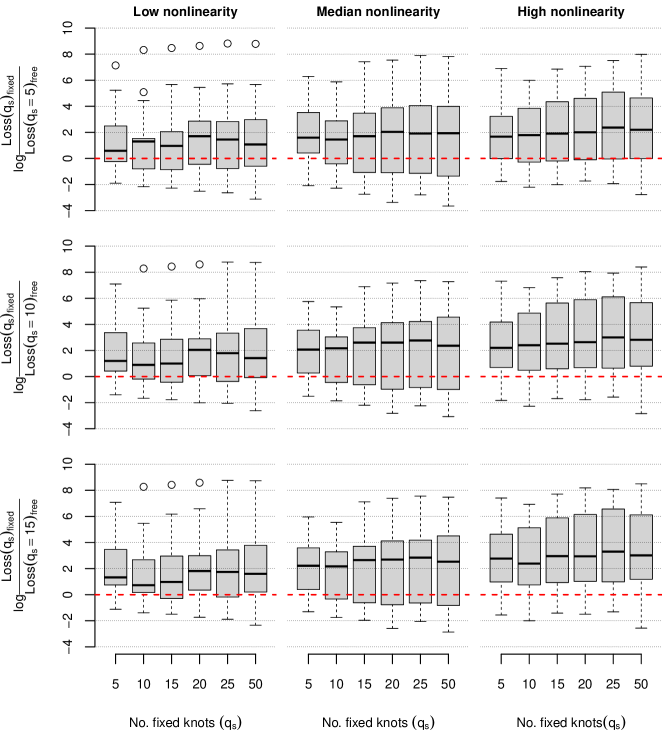
Figure 1. Boxplot of the log loss ratio comparing the performance of the fixed knots model with the free knots model for the DGP with $p=2$ and $n=200$. The three columns of the figure correspond to different degrees of nonlinearity of the realized datasets, as measured by estimated $\mathrm{DNL}$ in (5).

The aggregate results in Figure 1 do not clearly show how strikingly different the fixed and free knots models can perform on a given dataset. We will now show that models with free rather than fixed knots are much more robust across different datasets. Figure 2 displays the Euclidean distance of the multivariate out-of-sample predictive residuals $\sqrt{\tilde{\bm{\varepsilon}}^{\prime}\tilde{\bm{\varepsilon}}}$ for a few selected datasets as a function of the distance between the covariate vector and the sample mean of the covariates. The normed residuals depicted in the leftmost column are from datasets chosen with respect to the ranking of the out-of-sample performance of the fixed knots model. For example, the upper left subplot shows the predictive residuals of both the model with $15$ fixed knots (vertical bars above the zero line) and the model with $5$ free knots (vertical bars below the zero line) on one of the datasets where the fixed knot models outperform the free knots model by largest margin ($3$rd best Loss in favor of fixed knots model). It is seen from this subplot that even in this very favorably situation for the fixed knots model, the free knots model is not generating much larger predictive residuals. Moving down to the last row in the left hand column of Figure 2, we see the performance of the two models when the fixed knots model performs very poorly ($3$rd worse Loss with respect to the fixed knots model). On this particular dataset, the free knots model does well while the fixed knots model is a complete disaster (note the different scales on the vertical axes of the subplots). The column to the right in Figure 2 shows the same analysis, but this time the datasets are chosen with respect to the ranking of the Loss of the free knots model. Overall, Figure 2 clearly illustrates the superior robustness of models with free knots: the free knots model never does much worse than the fixed knots model, but using fixed rather than free knots can lead to a dramatically inferior predictive performance on individual datasets.

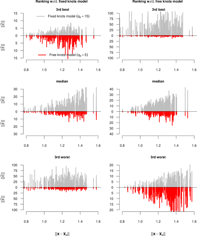
Figure 2. Plotting the norm of the predictive multivariate residuals as a function of the distance between the covariate vector and its sample mean. The results are for the DGP with $p=2$ and $n=200$. The lines in each subplot are the normed residuals from the model with $15$ fixed surface knots (vertical bars above the zero line), and the model with $5$ free knots (vertical bars below the zero line). The column to the left shows the results for three datasets chosen when performance is ranked according to the fixed knots model, and the right column displays the results for three datasets chosen when performance is ranked according to the free knots model.

4.3. Computing time

The program is written in native R code and all the simulations were performed on a Linux desktop with $2.8$ GHz CPU and $4$ GB RAM on single instance (without parallel computing). Table 1 shows the computing time in minutes for a single dataset. In general the computing time increases as the size of the design matrix increases, but it increases only marginally as we go from $p=1$ to $p=2$.

Table 1. Elapsed computing time (in minutes) for 5,000 iterations with a single dataset of $10$ covariates.

		$n=200$			$n=1000$
No. of free surface knots		$p=1$	$p=2$		$p=1$	$p=2$
$~{}2$		$~{}9$	$~{}9$		$16$	$17$
$~{}5$		$13$	$14$		$23$	$26$
$10$		$17$	$18$		$42$	$45$
$15$		$24$	$27$		$61$	$75$

5. Application to firm capital structure data

5.1. The data

The classic paper by Rajan & Zingales (1995) analyze firm leverage (leverage = total debt/(total debt + book value of equity)) as a function of its fixed assets (tang = tangible assets/book value of total assets), its market-to-book ratio (market2book = (book value of total assets - book value of equity + market value of equity)/book value of total assets), logarithm of sales (LogSale) and profit (Profit = earnings before interest, taxes, depreciation, and amortization/book value of total assets). Strong nonlinearities seem to be a quite general feature of balance sheet data, but only a handful articles have suggested using nonlinear/nonparametric models, see e.g. Bastos & Ramalho (2010), and Villani et al. (2012). We use a similar data to the one in Rajan & Zingales (1995) which covers $4,405$ American non-financial firms with positive sales in $1992$ and complete data records and analyze the leverage in terms of total debt. Villani et al. (2012) analyze the same data with a smooth mixture of Beta regressions.

Figure 3 plots the response variable leverage in both original scale and logit scale ($\ln[y/(1-y)]$) against each of the four covariates. The relationships between the leverage and the covariates are clearly highly nonlinear even when the logit transformation is used. There are also outliers which can be seen from the subplots with respect to covariates Market2Book and Profit.

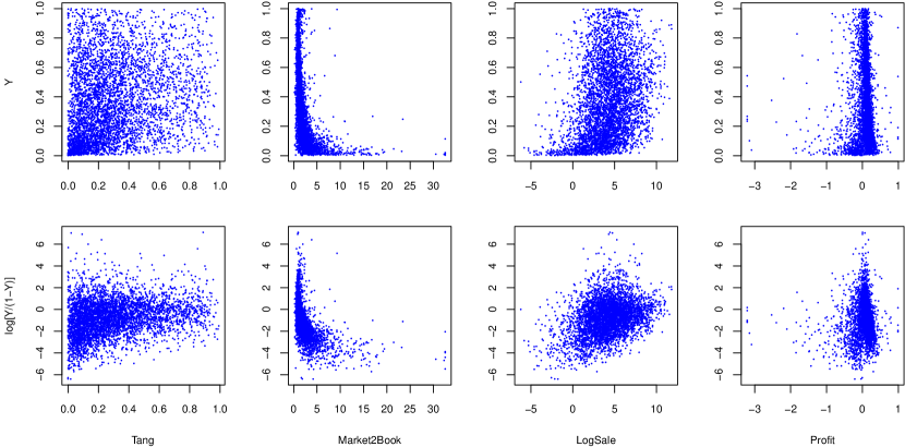
Figure 3. Scatter plots of the firm leverage data with leverage ($\bm{Y}$) on both original scale (top subplots) and logit transformed scale (bottom subplots) against each of the four covariates.

5.2. Models with only surface or additive components

We first fit models that either have only a surface component or only an additive component (both types of models also have a linear component). Note that the shrinkage parameters are also estimated in all cases. All four covariates are used in the estimation procedure and we use the logit transformation of the leverage, and standardize each covariate to have zero mean and unit variance.

Figure 4 depicts the LPDS for the surface component model and the additive component model for both the case of fixed and free knots. The LPDS generally improves as the number of knots increases for both the fixed and free knots models, but seems to eventually level off at large number of knots. The free knots model always outperforms the fixed knots model when only a surface component is used (left subplot). For example, the model with $12$ free surface knots is roughly $32$ LPDS units better than the fixed knots model with the same number of knots. This is a quite impressive improvement in out-of-sample performance considering that the fixed knot locations are chosen with state-of-the-art clustering methods for knot selection. The ability to move the knots clearly also helps to keep the number of knots to a minimum; it takes for example more than $30$ fixed surface knots to obtain the same LPDS as a model with $12$ free surface knots.

Turning to the strictly additive models in right subplot of Figure 4 we see that the additive models are in general inferior to the models with only surface knots, and that the differences in LPDS between the fixed and free knots approaches are much smaller here, at least for eight knots or more. The improvement in LPDS levels off at roughly $16$ knots. It is important to note that the horizontal axis in Figure 4 displays the number of additive knots in each covariate, and the fact that we do not overfit bear testimony to the effectiveness of the shrinkage priors.

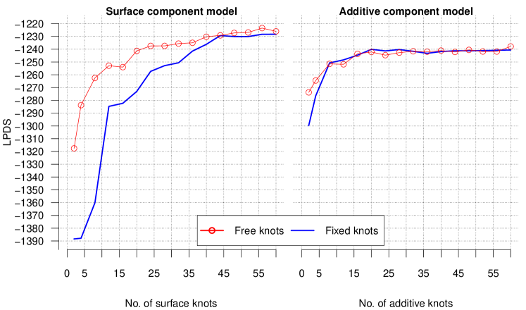
Figure 4. LPDS for the firm leverage data with surface component model (left) and additive component model (right). Note that the number of knots in additive model is the number of spline basis functions on each covariate.

5.3. Models with both additive and surface components

We now consider models with both additive and surface components. It is worth mentioning that we draw from the joint posterior distribution of the surface and additive knots, see Section A for MCMC details.

Figure 5 shows that there are generally improvements from using both surface knots and additive knots in the same model. For example, the model with $4$ free surface knots has an LPDS of $-1,284$. Adding two free additive knots increases the LPDS to $-1,270$ and adding another two additive knots gives a further increase of $14$ LPDS units. Figure 5 also shows strong gains from estimating the knots’ locations, but the improvement in LPDS from free knots tends to be less dramatic when more additive knots are used to complement the surface knots. There is little or no improvement in LPDS as the number of surface knots approaches $60$. The results in Figure 5 reinforces the evidence in Figure 4 that the shrinkage prior is very effective in mitigating potential problems with overfitting.

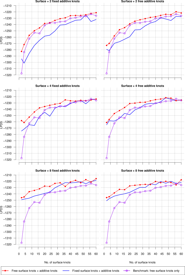
Figure 5. LPDS for the firm leverage data for the free and fixed knots models with varying number of surface and additive knots.

To simplify the graphical presentation of the results, we choose to illustrate the posterior inference of the knot locations in a model with only the two covariates Market2Book and Profit. We use $20$ surface knots and $4$ additive knots in each covariate. The mean acceptance probabilities for the knot locations and the shrinkage parameters in Metropolis-Hastings algorithm are $0.73$ and $0.64$, respectively, which are exceptionally large considering that all $2\times 20+2\times 4=48$ knot location parameters are proposed jointly, as are all the shrinkage parameters. The acceptance probability in the updating step for $\bm{\Sigma}$ is $1$ since we are proposing directly from the exact conditional posterior when $p=1$ . Because of the knot switching problem (see Section 3), it does not make much sense to display the posterior distribution of the knot locations directly. We instead choose to partition the covariate space into small rectangular regions, count the frequency of knots in each region over the MCMC iterations, and use heat maps to visualize the density of knots in different regions of covariate space. Figure 6 displays this knot density heat map. As expected, the estimated knot locations are mostly concentrated in the data dense regions, particularly in regions where the relation between the covariates and response in the data is most nonlinear, which is seen by comparing Figure 6 and Figure 3.

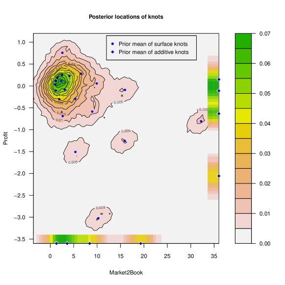
Figure 6. Heat map to visualize the posterior density of the knot locations in covariate space for model with $4$ free additive knots and $20$ free surface knots for the firm leverage dataset. The plot is constructed by partitioning the covariate space into $70\times 70$ rectangular regions and counting the number of surface knots in each rectangle over the MCMC draws. The posterior density of the locations of the additive knots is constructed in a similar fashion and separate heat maps for the additive knots in each covariate are shown just above the horizontal axis and vertical axis, respectively.

Finally, we present the posterior surface for the firm leverage data in Figure 7. To enhance the visual representation, the graphs zoom in on the region with the majority of the data observations. Figure 7 plots the mean (left) and the standard deviation (right) of the posterior surface. The latter object is for brevity sometimes referred to as the posterior standard deviation surface. Figure 7 (right) also displays the covariate observations to give a sense of where the data observations are located. The Supporting Information to this article investigates the robustness of the posterior results to variations in both the prior mean and variance of the knot locations. The posterior heat map of the knot locations are affected by the fairly dramatic variations in the prior mean of the knots, and to a lesser extent by changes in the prior variance of the knot locations, but the posterior mean and standard deviation surfaces are robust to variations in the prior on the knots, especially in data dense regions. The Supporting Information also shows that the posterior is robust to changes in the prior on the shrinkage factors.

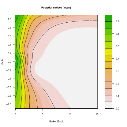
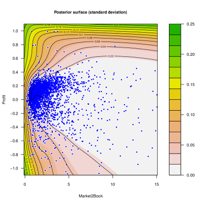
Figure 7. The posterior mean (left) and standard deviation (right) of the posterior surface for the model with $4$ free additive knots and $20$ free surface knots for firm leverage data. The subplot to the right also shows an overlay of the covariate observations.

5.4. MCMC efficiency in the updating of the knot locations

In order to study the efficiency of our algorithm for sampling the knot locations, we compare three types of MCMC updates of the knots: i) one-knot-at-a-time updates using a random walk Metropolis proposal with tuned variance (SRWM), ii) one-knot-at-a-time updates with the tailored Metropolis-Hastings step (SMH) in Section 3.2, and iii) full block updating of all knots using the tailored Metropolis-Hastings step (BMH) in Section 3.2. SRWM moves are used in state-of-the-art RJMCMC approaches such as Dimatteo et al. (2001) and Gulam Razul et al. (2003). Note that we are not studying the performance of a complete RJMCMC scheme; we are here interested in isolating this particular updating step and comparing it to our tailored proposal. We use the inefficiency factor (IF) (Geweke, 1992) to measure the efficiency of MCMC. The IF is a measure of the number of draws needed to obtain the equivalent of a single independent draw. It is defined as $\mathrm{IF}=1+2\sum_{i=1}^{\infty}\rho_{i}$ where $\rho_{i}$ is the autocorrelation of the MCMC trajectory at lag $i$. We also document the effective sample size per minute, i.e. $(\text{number of MCMC draws})/(\text{IF}\times\text{computing time})$ to measure the overall efficiency of the MCMC.

Table 2 shows the efficiency of the three knot sampling algorithms in a model with $20$ free surface knots and $4$ additive knots in each covariate on the firm leverage data. The inefficiency factor in Table 2 is the average inefficiency of the posterior mean surface in $1000$ random chosen points in covariate space. There is some gain from tailoring the proposal for each knot separately, but the really striking observation from Table 2 is the massive efficiency and speed gains from updating all the blocks jointly using a tailored proposal; the effective sample size per minute is roughly $70$ times larger when our BMH algorithm is used instead of simple SRWM updates.

Table 2. Comparison of algorithms for updating the knot locations in a model with $20$ free surface knots and $4$ additive knots in each covariate. Firm leverage data.

		SRWM		SMH		BMH
Mean IF for the posterior mean surface		$29.63$		$2.70$		$1.16$
Mean acceptance probability		$0.26$		$0.62$		$0.88$
Computing time (min)		$388.21$		$1716.07$		$141.72$
Effective sample size per minute		$0.87$		$2.16$		$60.83$

6. Concluding remarks

We have presented a general Bayesian approach for fitting a flexible surface model for a continuous multivariate response using a radial basis spline with freely estimated knot locations. Our approach uses shrinkage priors to avoid overfitting. The locations of the knots and the shrinkage parameters are treated as unknown parameters and we propose a highly efficient MCMC algorithm for these parameters with the coefficients of the multivariate spline integrated out analytically. An important feature of our algorithm is that all knot locations are sampled jointly using a Metropolis-Hastings proposal density tailored to the conditional posterior, rather than the one-knot-at-a-time random walk proposals used in previous literature. The same applies to the block of shrinkage parameters. Both a simulation study and a real application on firm leverage data show that models with free knots have a better out-of-sample predictive performance than models with fixed knots. Moreover, the free knots model is also more robust in the sense that it performs consistently well across different datasets. We also found that models that mix surface and additive spline basis functions in the same model perform better than models with only one of the two basis types.

Our approach can be directly used with other splines basis functions, other priors, and it is at least in principle straightforward to augment the model with Bayesian variable selection. Also, the assumption of Gaussian error distribution could be easily removed by using a Dirichlet process mixture (DPM) prior. We would still be able to integrate out the regression coefficients if we assume a Gaussian base measure in the DPM, see Leslie et al. (2007) for details in the univariate case.

7. Acknowledgements

The authors are grateful to Paolo Giordani and Robert Kohn for stimulating discussions and constructive suggestions. The authors thank two anonymous referees for the helpful comments that improved the contents and presentation of the paper. The computations were performed on resources provided by SNIC through Uppsala Multidisciplinary Center for Advanced Computational Science (UPPMAX) under Project p2011229.

Appendix A Details of the MCMC algorithm

In this section we briefly address the MCMC details and related computational issues. For details on matrix manipulations and derivatives, see e.g. Lütkepohl (1996). Our MCMC algorithm in Section 3.2 only requires the gradient of the conditional posteriors w.r.t. each parameter. Since users can always use their own prior on the knots and shrinkages, we will not document the gradient of any particular prior. In particular for the normal prior, one can directly find the results in e.g. Mardia et al. (1979). We now present the full gradients for the knot locations and the shrinkage parameters.

A.1. Gradient w.r.t. the knot locations

$$\begin{split}\frac{{\partial\ln p\left({\bm{\xi}|\bm{\lambda},\bm{\Sigma},\bm{Y},\bm{X}}\right)}}{{\partial\bm{\xi}^{\prime}}}=&~{}\frac{{\partial\log p(\bm{\xi})}}{{\partial\bm{\xi}^{\prime}}}-\frac{p}{2}\sum\limits_{i\in\{o,a,s\}}{\left(\mathrm{vec}{\bm{P}_{i}}\right)}^{\prime}\frac{{\partial\mathrm{vec}{\bm{P}_{i}}}}{{\partial\bm{\xi}^{\prime}}}\\ &-\left({\bm{\tilde{\beta}}-\bm{\mu}}\right)^{\prime}\bm{\Sigma}_{\bm{\beta}}^{-1}\frac{{\partial\bm{\tilde{\beta}}}}{{\partial\bm{\xi}^{\prime}}}-\frac{1}{2}\left(\mathrm{vec}{\bm{\Sigma}_{\bm{\tilde{\beta}}}}\right)^{\prime}\frac{{\partial\mathrm{vec}{\bm{[}{\Sigma}^{-1}}\otimes\bm{X}^{\prime}\bm{X}]}}{{\partial\bm{\xi}^{\prime}}}\hfill\\ &-\frac{1}{2}\left(\mathrm{vec}{\bm{\Sigma}^{-1}}\right)^{\prime}\left({{\bm{I}_{p}}+{\bm{K}_{p,p}}}\right)\left\{{({\bm{I}_{p}}\otimes\bm{\tilde{E}}^{\prime}\bm{X})\frac{{\partial\bm{\tilde{\beta}}}}{{\partial\bm{\xi}^{\prime}}}+(\bm{\tilde{B}}^{\prime}\otimes\bm{\tilde{E}}^{\prime})\frac{{\partial\mathrm{vec}\bm{X}}}{{\partial\bm{\xi}^{\prime}}}}\right\}\hfill\\ &-\frac{1}{2}\left\{\mathrm{vec}\left[{\left({\bm{\tilde{\beta}}-\bm{\mu}}\right)\left({\bm{\tilde{\beta}}-\bm{\mu}}\right)^{\prime}+\bm{\Sigma}_{\bm{\tilde{\beta}}}}\right]\right\}^{\prime}\frac{{\partial\mathrm{vec}\bm{\Sigma}_{\bm{\beta}}^{-1}}}{{\partial\bm{\xi}^{\prime}}},\hfill\end{split}$$

where $\bm{\tilde{E}}=\bm{Y}-\bm{X\tilde{B}}$, $\bm{I}_{p}$ is the identity matrix, $\bm{K}_{p,p}$ is the commutation matrix and

$$\frac{{\partial\mathrm{vec}[{\bm{\Sigma}^{-1}}\otimes\bm{X}^{\prime}\bm{X}]}}{{\partial\bm{\xi}^{\prime}}}=\left({{\bm{I}_{p}}\otimes{\bm{K}_{q,p}}\otimes{\bm{I}_{q}}}\right)\left({\mathrm{vec}{\bm{\Sigma}^{-1}}\otimes{\bm{I}_{{q^{2}}}}}\right)\left({{\bm{I}_{{q^{2}}}}+{\bm{K}_{q,q}}}\right)\left({{\bm{I}_{q}}\otimes\bm{X}^{\prime}}\right)\frac{{\partial\mathrm{vec}\bm{X}}}{{\partial\bm{\xi}^{\prime}}},$$

$$\begin{split}\frac{{\partial\bm{\tilde{\beta}}}}{{\partial\bm{\xi}^{\prime}}}=~{}&{\bm{\Sigma}_{\bm{\tilde{\beta}}}}\left[{\left[{{\bm{\Sigma}^{-1}}\bm{Y}^{\prime}\otimes{\bm{I}_{q}}}\right]{\bm{K}_{n,q}}\frac{{\partial\mathrm{vec}\bm{X}}}{{\partial\bm{\xi}^{\prime}}}+\left({\bm{\mu}^{\prime}\otimes{\bm{I}_{pq}}}\right)\frac{{\partial\mathrm{vec}\bm{\Sigma}_{\bm{\beta}}^{-1}}}{{\partial\bm{\xi}^{\prime}}}}\right]\hfill\\ &-\left[\left\{{\left[{\mathrm{vec}\left({\bm{X}^{\prime}\bm{Y}{\bm{\Sigma}^{-1}}}\right)+\bm{\Sigma}_{\bm{\beta}}^{-1}\bm{\mu}}\right]^{\prime}{\bm{\Sigma}_{\bm{\tilde{\beta}}}}}\right\}\otimes{\bm{\Sigma}_{\bm{\tilde{\beta}}}}\right]\left[{\frac{{\partial\mathrm{vec}[{\bm{\Sigma}^{-1}}\otimes\bm{X}^{\prime}\bm{X}]}}{{\partial\bm{\xi}^{\prime}}}+\frac{{\partial\mathrm{vec}\bm{\Sigma}_{\bm{\beta}}^{-1}}}{{\partial\bm{\xi}^{\prime}}}}\right].\hfill\end{split}$$

We can decompose the gradient for the design matrix w.r.t the knots as

$$\frac{{\partial\mathrm{vec}\bm{X}}}{{\partial\bm{\xi}^{\prime}}}=\left[{\begin{array}[]{ll}\bm{0}_{(nq_{o}\times l_{s})}&{\bm{0}_{(nq_{o}\times l_{a})}}\\ \partial\mathrm{vec}{\bm{X}_{s}}/\partial{\mathrm{vec}(\bm{\xi}_{s}^{\prime})}^{\prime}&{\bm{0}_{(nq_{s}\times l_{a})}}\\ {\bm{0}_{(nq_{a}\times l_{s})}}&\partial\mathrm{vec}{\bm{X}_{a}}/\partial{\bm{\xi}_{a}}^{\prime}\end{array}}\right]$$

where $l_{s}$ and $l_{a}$ are numbers of parameters in the knots locations for surface and additive component, respectively. This decomposition makes user-specified basis functions for different components possible and one may update the locations in a parallel mode (efficient for small models) or batched mode (for models with many parameters). In particular for the thin-plate spline, we have

$$\frac{{\partial{\text{vec}}{{\bm{X}}_{i}}}}{{\partial{\bm{\xi}_{i}}^{\prime}}}=-{\left[{\begin{array}[]{ccc}{({1+2\ln\|{{{\bm{x}}_{i}}-{\bm{\xi}_{ij}}}\|})({{{\bm{x}}_{i}}-{\bm{\xi}_{ij}}})}&{}\hfil&{}\hfil\\ {}\hfil&\ddots&{}\hfil\\ {}\hfil&{}\hfil&{({1+2\ln\|{{{\bm{x}}_{i}}-{\bm{\xi}_{ij}}}\|})({{{\bm{x}}_{i}}-{\bm{\xi}_{ij}}})}\end{array}}\right]{\begin{subarray}{l}\vspace{1.5cm}\\ i\in\{a,s\},\\ j\in\{1,...,{q_{i}}\}.\end{subarray}}}$$

Note that the gradient can be obtained efficiently by applying Lemma A.1 and Algorithm A.1 in Section A.3 below whenever $\partial\mathrm{vec}\bm{\Sigma}_{\bm{\beta}}^{-1}/\partial\bm{\xi}^{\prime}$ and the commutation matrix appear.

A.2. Gradient w.r.t. the shrinkage parameters

$$\begin{split}\frac{{\partial\ln p\left({\bm{\lambda}|\bm{\xi},\bm{\Sigma},\bm{Y},\bm{X}}\right)}}{{\partial\bm{\lambda}^{\prime}}}=&~{}\frac{{\partial\log p(\bm{\lambda})}}{{\partial\bm{\lambda}^{\prime}}}-\frac{1}{2}\left[{{q_{o}}{\bm{\lambda}_{o}}^{\prime},{q_{s}}{\bm{\lambda}_{s}}^{\prime},{q_{a}}{\bm{\lambda}_{a}}^{\prime}}\right]-\left(\bm{\tilde{\beta}}-\bm{\mu}\right)^{\prime}\bm{\Sigma}_{\bm{\beta}}^{-1}\frac{\partial\bm{\tilde{\beta}}}{\partial\bm{\lambda}^{\prime}}\\ &-\frac{1}{2}\left(\mathrm{vec}{\bm{\Sigma}^{-1}}\right)^{\prime}\left({{\bm{I}_{p}}+{\bm{K}_{p,p}}}\right)\left({{\bm{I}_{p}}\otimes\bm{\tilde{E}}^{\prime}\bm{X}}\right)\frac{{\partial\bm{\tilde{\beta}}}}{{\partial\bm{\lambda}^{\prime}}}\hfill\\ &-\frac{1}{2}\mathrm{vec}\left[{\left({\bm{\tilde{\beta}}-\bm{\mu}}\right)\left({\bm{\tilde{\beta}}-\bm{\mu}}\right)^{\prime}+{\mathrm{\Sigma}_{\bm{\tilde{\beta}}}}}\right]^{\prime}\frac{{\partial\mathrm{vec}\bm{\Sigma}_{\bm{\beta}}^{-1}}}{{\partial\bm{\lambda}^{\prime}}},\hfill\end{split}$$

where

$$\frac{{\partial\bm{\tilde{\beta}}}}{{\partial\bm{\lambda}^{\prime}}}=\left\{{\left[{\left({\mathrm{vec}\left({\bm{X}^{\prime}\bm{Y}{\bm{\Sigma}^{-1}}}\right)+\bm{\Sigma}_{\bm{\beta}}^{-1}\bm{\mu}}\right)^{\prime}{\bm{\Sigma}_{\bm{\tilde{\beta}}}}}\right]\otimes{\bm{\Sigma}_{\bm{\beta}}}-\bm{\mu}^{\prime}\otimes{\bm{\Sigma}_{\bm{\tilde{\beta}}}}}\right\}\frac{{\partial\mathrm{vec}\bm{\Sigma}_{\bm{\beta}}^{-1}}}{{\partial\bm{\lambda}^{\prime}}},$$

and $\partial\mathrm{vec}\bm{\Sigma}_{\bm{\beta}}^{-1}/\partial\bm{\lambda}^{\prime}$ can be obtained efficiently by applying Lemma A.1 in Section A.3 and by

$$\begin{split}\frac{{\partial\mathrm{vec}[({\bm{\bm{\Lambda}}_{i}^{-1/2}}{\bm{\Sigma}^{-1}}{\bm{\bm{\Lambda}}_{i}^{-1/2}})\otimes{\bm{P}_{i}}]}}{{\partial{\bm{\lambda}_{i}}^{\prime}}}=~{}&\left({{\bm{I}_{p}}\otimes{\bm{K}_{{q_{i}},p}}\otimes{\bm{I}_{{q_{i}}}}}\right)\left({{\bm{I}_{{p^{2}}}}\otimes\mathrm{vec}{\bm{P}_{i}}}\right)\left({{\bm{I}_{{p^{2}}}}+{\bm{K}_{p,p}}}\right)\hfill\\ &\times\left({{\bm{I}_{p}}\otimes[{\bm{\bm{\Lambda}}_{i}^{-1/2}}{\bm{\Sigma}^{-1}}]}\right)\frac{\partial\mathrm{vec}\bm{\Lambda}_{i}^{-1/2}}{\partial\bm{\lambda}_{i}^{\prime}},~{}i\in\{a,s\}.\hfill\end{split}$$

where $\partial\mathrm{vec}\bm{\Lambda}_{i}/\partial\bm{\lambda}_{i}^{\prime}$ is $p^{2}\times p$ matrix with elements $\nabla_{j(p+1)-p,~{}j}=-1/2\lambda_{i,j}^{-3/2}$ for $j=1,...,p$ and zero elsewhere.

A.3. Computational remarks

The computational implementation of gradients in Section A.1 and Section A.2 is straightforward but the sparsity of some of the matrices can be exploited in moderate to large datasets. We now present a lemma and an algorithm that can dramatically speed up the computations. It is convenient to define $\bm{A}(\bm{i},\textnormal{:})$ and $\bm{A}(:,\bm{j})$ as matrix operations that reorders the rows and columns of matrix $\bm{A}$ with indices $\bm{i}$ and $\bm{j}$. Therefore, $\bm{\beta}=\bm{b}(\bm{c},:)$, $\bm{\mu}=\bm{\mu}^{*}(\bm{c},:)$ and $\bm{\Sigma}_{\bm{\beta}}=\bm{\Sigma}_{\bm{b}}(\bm{c},\bm{c})$ for proper indices $\bm{c}$, and $|\bm{\Sigma}_{\bm{b}}|=|\bm{\Sigma}_{\bm{\beta}}|$ since permuting two rows or columns changes the sign but not the magnitude of the determinant.

Lemma A.1.

Given matrix $\bm{C}$ and the indexing vector $\bm{z}$ such that $(\mathrm{vec}\bm{\Sigma}_{\bm{b}})(\bm{z},:)=\mathrm{vec}\bm{\Sigma}_{\bm{\beta}}$ holds, we can decompose the following gradient as

$$\bm{C}\frac{{\partial\mathrm{vec}[\bm{\Sigma}_{\bm{\beta}}^{-1}\left(\bm{\theta}\right)]}}{{\partial\bm{\theta}}^{\prime}}=\left[{{\bm{C}_{s}}\frac{{\partial\mathrm{vec}[(\bm{\Lambda}_{s}^{-1/2}\bm{\Sigma}^{-1}\bm{\Lambda}_{s}^{-1/2})\otimes{\bm{P}_{s}}]}}{{\partial{\bm{\theta}_{s}}^{\prime}}},~{}{\bm{C}_{a}}\frac{{\partial\mathrm{vec}[({\bm{\Lambda}_{a}^{-1/2}\bm{\Sigma}^{-1}\bm{\Lambda}_{a}^{-1/2}})\otimes{\bm{P}_{a}}]}}{{\partial{\bm{\theta}_{a}}^{\prime}}}}\right]$$

where $\bm{\theta}$ is any parameter vector of the covariance matrix $\bm{\Sigma}_{\bm{\beta}}$, $\bm{C}_{s}=\{[\bm{C}(:,\bm{z})](:,\bm{h}_{s})\}(:,\bm{z}_{s}\neq 0)$, $\bm{h}_{s}=[(p^{2}qq_{o}+1),(p^{2}qq_{o}+2),...,p^{2}q(q_{o}+q_{s})]^{\prime}$, $\bm{z}_{s}=\mathrm{vec}([\bm{0}_{pq_{s}\times pq_{o}},~{}\bm{1}_{pq_{s}\times pq_{s}},~{}\bm{0}_{pq_{s}\times pq_{a}}]^{\prime})$, $\bm{C}_{a}=\{[\bm{C}(:,\bm{z})](:,\bm{h}_{a})\}(:,\bm{z}_{a}\neq 0)$, $\bm{h}_{a}=[(p^{2}q(q_{o}+q_{s})+1),(p^{2}q(q_{o}+q_{s})+2),...,p^{2}q^{2}]^{\prime}$ and $\bm{z}_{a}=\mathrm{vec}([\bm{0}_{pq_{a}\times p(q_{o}+q_{s})},~{}\bm{1}_{pq_{a}\times pq_{a}}]^{\prime})$.

Algorithm A.1.

An efficient algorithm to calculate $\bm{K}_{m,n}\bm{Q}$ (or $\bm{Q}\bm{K}_{m,n}$) where $\bm{K}_{m,n}$ is the commutation matrix and $\bm{Q}$ is any dense matrix that is conformable to $\bm{K}_{m,n}$.

1. Create an $m\times n$ (or $n\times m$) matrix $\bm{T}$ and fill it by columns with the sequence $\{1,2,...,nm\}$.

2. Obtain the indexing vector $\bm{t}=\mathrm{vec}(\bm{T}^{\prime})$.

3. Return $\bm{Q}(\bm{t},:)$ (or $\bm{Q}(:,\bm{t})$).

References

- (1)
- Bastos & Ramalho (2010) Bastos, J. & Ramalho, J. (2010), ‘Nonparametric models of financial leverage decisions’, CEMAPRE Working Papers . Available at: http://cemapre.iseg.utl.pt/archive/preprints/426.pdf.
- Breiman et al. (1984) Breiman, L., Friedman, J., Olshen, R. & Stone, C. (1984), Classification and regression trees, Chapman and Hall/CRC, New York.
- Buhmann (2003) Buhmann, M. (2003), Radial basis functions: theory and implementations, Cambridge University Press, Cambridge.
- Chipman et al. (2010) Chipman, H., George, E. & McCulloch, R. (2010), ‘BART: Bayesian additive regression trees’, The Annals of Applied Statistics 4(1), 266–298.
- Denison et al. (2002) Denison, D., Holmes, C. C., Mallick, B. K. & Smith, A. F. M. (2002), Bayesian Methods for Nonlinear Classification and Regression, Jone Wiley & Sons, Chichester.
- Denison et al. (1998) Denison, D., Mallick, B. & Smith, A. (1998), ‘Automatic Bayesian curve fitting’, Journal of the Royal Statistical Society: Series B (Statistical Methodology) 60(2), 333–350.
- Dimatteo et al. (2001) Dimatteo, I., Genovese, C. & Kass, R. (2001), ‘Bayesian curve-fitting with free-knot splines’, Biometrika 88(4), 1055–1071.
- Friedman (1991) Friedman, J. (1991), ‘Multivariate adaptive regression splines’, The Annals of Statistics 19(1), 1–67.
- Gamerman (1997) Gamerman, D. (1997), ‘Sampling from the posterior distribution in generalized linear mixed models’, Statistics and Computing 7(1), 57–68.
- Gasser & Müller (1979) Gasser, T. & Müller, H. (1979), Kernel estimation of regression functions, in T. Gasser & M. Rosenblatt, eds, ‘Smoothing Techniques for Curve Estimation’, Vol. 757, Springer, New York, pp. 23–68.
- Geweke (1992) Geweke, J. (1992), Evaluating the accuracy of sampling-based approaches to the calculation of posterior moments, in J. M. Bernardo, J. O. Berger, A. P. David & A. F. M. Smith, eds, ‘Bayesian Statistics 4’, Oxford University Press, Oxford, pp. 169–193.
- Geweke (2007) Geweke, J. (2007), ‘Interpretation and inference in mixture models: Simple MCMC works’, Computational Statistics & Data Analysis 51(7), 3529–3550.
- Geweke & Amisano (2011) Geweke, J. & Amisano, G. (2011), ‘Optimal prediction pools’, Journal of Econometrics 164(1), 130–141.
- Gulam Razul et al. (2003) Gulam Razul, S., Fitzgerald, W. & Andrieu, C. (2003), ‘Bayesian model selection and parameter estimation of nuclear emission spectra using RJMCMC’, Nuclear Instruments and Methods in Physics Research Section A: Accelerators, Spectrometers, Detectors and Associated Equipment 497(2-3), 492–510.
- Hastie & Tibshirani (1990) Hastie, T. & Tibshirani, R. (1990), Generalized additive models, Chapman & Hall/CRC, New York.
- Hastie et al. (2009) Hastie, T., Tibshirani, R. & Friedman, J. (2009), The Elements of Statistical Learning: Data Mining, Inference, and Prediction, Springer, New York.
- Holmes & Mallick (2003) Holmes, C. & Mallick, B. (2003), ‘Generalized nonlinear modeling with multivariate free-knot regression splines’, Journal of the American Statistical Association 98(462), 352–368.
- Kass (1993) Kass, R. (1993), ‘Bayes factors in practice’, The Statistician 42(5), 551–560.
- Khatri & Rao (1968) Khatri, C. & Rao, C. (1968), ‘Solutions to some functional equations and their applications to characterization of probability distributions’, Sankhyā: The Indian Journal of Statistics, Series A 30(2), 167–180.
- Leslie et al. (2007) Leslie, D., Kohn, R. & Nott, D. (2007), ‘A general approach to heteroscedastic linear regression’, Statistics and Computing 17(2), 131–146.
- Lütkepohl (1996) Lütkepohl, H. (1996), Handbook of matrices, John Wiley & Sons, Chichester.
- Mardia et al. (1979) Mardia, K., Kent, J., & Bibby, J. (1979), Multivariate analysis, Academic Press, London.
- Nadaraya (1964) Nadaraya, E. A. (1964), ‘On estimating regression’, Theory of Probability and its Applications 9, 141–142.
- Nott & Leonte (2004) Nott, D. & Leonte, D. (2004), ‘Sampling schemes for Bayesian variable selection in generalized linear models’, Journal of Computational and Graphical Statistics 13(2), 362–382.
- Rajan & Zingales (1995) Rajan, R. & Zingales, L. (1995), ‘What do we know about capital structure? Some evidence from international data’, Journal of Finance 50(5), 1421–1460.
- Richardson & Green (1997) Richardson, S. & Green, P. (1997), ‘On Bayesian analysis of mixtures with an unknown number of components (with discussion)’, Journal of the Royal Statistical Society: Series B (Statistical Methodology) 59(4), 731–792.
- Ruppert et al. (2003) Ruppert, D., Wand, M. & Carroll, R. (2003), Semiparametric regression, Cambridge University Press, Cambridge.
- Smith & Kohn (1996) Smith, M. & Kohn, R. (1996), ‘Nonparametric regression using Bayesian variable selection’, Journal of Econometrics 75(2), 317–343.
- Tibshirani (1996) Tibshirani, R. (1996), ‘Regression shrinkage and selection via the lasso’, Journal of the Royal Statistical Society. Series B (Methodological) pp. 267–288.
- Villani et al. (2012) Villani, M., Kohn, R. & Nott, D. J. (2012), ‘Generalized Smooth Finite Mixtures’, Journal of Econometrics . Forthcoming, available at: http://dx.doi.org/10.1016/j.jeconom.2012.06.012.
- Watson (1964) Watson, G. (1964), ‘Smooth regression analysis’, Sankhyā: The Indian Journal of Statistics, Series A 26(4), 359–372.
- Wood et al. (2002) Wood, S., Jiang, W. & Tanner, M. (2002), ‘Bayesian mixture of splines for spatially adaptive nonparametric regression’, Biometrika 89(3), 513.
- Zellner (1971) Zellner, A. (1971), An introduction to Bayesian inference in econometrics, John Wiley & Sons, New York.
- Zellner (1986) Zellner, A. (1986), ‘On assessing prior distributions and Bayesian regression analysis with g-prior distributions’, Bayesian Inference and Decision Techniques: Essays in Honor of Bruno de Finetti 6, 233–243.