Theory of quasi-spherical accretion in X–ray pulsars

Abstract

A theoretical model for quasi-spherical subsonic accretion onto slowly rotating magnetized neutron stars is constructed. In this model the accreting matter subsonically settles down onto the rotating magnetosphere forming an extended quasi-static shell. This shell mediates the angular momentum removal from the rotating neutron star magnetosphere during spin-down episodes by large-scale convective motions. The accretion rate through the shell is determined by the ability of the plasma to enter the magnetosphere. The settling regime of accretion can be realized for moderate accretion rates $\dot{M}<\dot{M}_{*}\simeq 4\times 10^{16}$ g/s. At higher accretion rates a free-fall gap above the neutron star magnetosphere appears due to rapid Compton cooling, and accretion becomes highly non-stationary. From observations of the spin-up/spin-down rates (the angular rotation frequency derivative $\dot{\omega}^{*}$, and $\partial\dot{\omega}^{*}/\partial\dot{M}$ near the torque reversal) of X-ray pulsars with known orbital periods, it is possible to determine the main dimensionless parameters of the model, as well as to estimate the magnetic field of the neutron star. We illustrate the model by determining these parameters for three wind-fed X-ray pulsars GX 301-2, Vela X-1, and GX 1+4. The model explains both the spin-up/spin-down of the pulsar frequency on large time-scales and the irregular short-term frequency fluctuations, which can correlate or anti-correlate with the X-ray flux fluctuations in different systems. It is shown that in real pulsars an almost iso-angular-momentum rotation law with $\omega\sim 1/R^{2}$, due to strongly anisotropic radial turbulent motions sustained by large-scale convection, is preferred.

1 Introduction

X-ray pulsars are highly magnetized neutron stars in binary systems, accreting matter from a companion star. The companion may be a low-mass star overfilling its Roche lobe in which case an accretion disc is formed. In the case of a high-mass companion, the neutron star may also accrete from the strong stellar wind and depending on the conditions a disc may be formed or accretion may take place quasi-spherically. The strong magnetic field of the neutron star disrupts the accretion flow at some distance from the neutron star surface and forces the accreted matter to funnel down on the polar caps of the neutron star creating hot spots that, if misaligned with the rotational axis, make the neutron star pulsate in X-rays. Most accreting pulsars show stochastic variations in their spin frequencies as well as in their luminosities. Many sources also exhibit long-term trends in their spin-behaviour with the period more or less steadily increasing or decreasing and in some sources spin-reversals have been observed. (For a thorough review, see e.g. Bildsten 1997 and references therein.)

The best-studied case of accretion is that of thin disc accretion (Shakura & Sunyaev 1973). Here the spin-up/spin-down mechanisms are rather well understood. For disc accretion the spin-up torque is determined by the specific angular momentum at the inner edge of the disc and can be written in the form $K_{su}\approx\dot{M}\sqrt{GMR_{A}}\,$ (Pringle and Rees, 1972). For a pulsar the inner radius of the accretion disc is determined by the Alfven radius $R_{A}$, $R_{A}\sim\dot{M}^{-2/7}$, so $K_{su}\sim\dot{M}^{6/7}$, i.e. for disc accretion the spin-up torque is weakly (almost linearly) dependent on the accretion rate (X-ray luminosity). In contrast, the spin-down torque for disc accretion in the first approximation is independent of $\dot{M}$: $K_{sd}\sim-\mu^{2}/R_{c}^{3}$, where $R_{c}=(GM/(\omega^{*})^{2})^{1/3}$ is the corotation radius, $\omega^{*}$ is the neutron star angular frequency and $\mu$ is the neutron star’s dipole magnetic moment. In fact, accretion torques in disc accretion are determined by a complicated disc-magnetospheric interaction, see, e.g., Ghosh & Lamb (1979), Lovelace et al. (1995) and the discussion in Kluźniak & Rappaport (2007), and correpsondingly can have a more complicated dependence on the mass accretion rate and other parameters.

Measurements of spin-up/spin-down in X-ray pulsars can be used to evaluate a very important parameter of the neutron star – its magnetic field. The period of the pulsar is usually close to the equilibrium value $P_{eq}$, which is determined by the total zero torque applied to the neutron star, $K=K_{su}+K_{sd}=0$. So assuming the observed value $\omega^{*}=2\pi/P_{eq}$, the magnetic field of the neutron star in disc-accreting X-ray pulsars can be estimated if $\dot{M}$ is known.

In the case of quasi-spherical accretion, which can take place in systems where the optical star underfills its Roche lobe and no accretion disc is formed, the situation is more complicated. Clearly, the amount and sign of the angular mometum supplied to the neutron star from the captured stellar wind are important for spin-up or spin-down. To within a numerical factor (which can be positive or negative, see numerical simulations by Fryxell & Taam (1988), Ruffert (1997), Ruffert (1999), etc.), the torque applied to the neutron star in this case should be proportional to $\dot{M}\omega_{B}R_{B}^{2}$, where $\omega_{B}=2\pi/P_{B}$ is the binary orbital angular frequency, $R_{B}=2GM/(V_{w}^{2}+v_{orb}^{2})^{2}$ is the gravitational capture (Bondi) radius, $V_{w}$ is the stellar wind velocity at the neutron star orbital distance, and $v_{orb}$ is the neutron star orbital velocity. In real high-mass X-ray binaries the orbital eccentricity is non-zero, the stellar wind is variable and can be inhomogeneous, etc., so $K_{su}$ can be a complicated function of time. The spin-down torque is even more uncertain, since it is impossible to write down a simple equation like $-\mu^{2}/R_{c}^{3}$ any more ($R_{c}$ has no meaning for quasi-spherical accretion; for slowly rotating pulsars it is much larger than the Alfven radius where the angular momentum transfer from the accreting matter to the magnetosphere actually occurs). For example, if one uses for the braking torque $-\mu^{2}/R_{c}^{3}$, the magnetic field in long-period X-ray pulsars turns out very high. We think this is a result of underestimating the braking torque.

The matter captured from the stellar wind can accrete onto the neutron star in different ways. Indeed, if the X-ray flux from the accreting neutron star is sufficiently high, the shocked matter rapidly cools down due to Compton processes and freely falls down toward the magnetosphere. The velocity of motion rapidly becomes supersonic, so a shock is formed above the magnetosphere. This regime was considered, e.g., by Burnard et al. (1983). Depending on the sign of the specific angular momentum of falling matter (prograde or retrograde), the neutron star can spin-up or spin-down. However, if the X-ray flux at the Bondi radius is below some value, the shocked matter remains hot, the radial velocity of the plasma is subsonic, and the settling accretion regime sets in. A hot quasi-static shell forms around the magnetosphere (Davies & Pringle, 1981). Due to additional energy release (especially near the base of the shell), the temperature gradient across the shell becomes superadiabatic, so large-scale convective motions inevitably appear. The convection intitiates turbulence, and the motion of a fluid element in the shell becomes quite complicated. If the magnetosphere allows plasma entry via instabilities (and subsequent accretion onto the neutron star), the actual accretion rate through such a shell is controlled by the magnetosphere (for example, the shell can exist, but the accretion through it can be weak or even absent altogether). So on top of the convective motions, the mean radial velocity of matter toward the magnetosphere, a subsonic settling, appears. This picture of accretion is realized at relatively small X-ray luminositites, $L_{x}<4\times 10^{36}$ erg/s (see below), and is totally different from what was considered in numerical simulations cited above. If the shell is present, its interaction with the rotating magnetosphere can lead to spin-up or spin-down of the neutron star, depending on the sign of the angular velocity difference between the accreting matter and the magnetospheric boundary. So in the settling accretion regime, both spin-up or spin-down of the neutron star is possible, even if the sign of the specific angular momentum of captured matter is prograde. The shell here mediates the angular momentum transfer to or from the rotating neutron star.

One can find several models in the literature (see especially Illarionov & Kompaneets 1990 and Bisnovatyi-Kogan 1991), from which the expression for the spin-down torque for quasi-spherically accreting neutron stars in the form $K_{sd}\sim-\dot{M}R_{A}^{2}\omega^{*}\sim-\dot{M}^{3/7}$ can be derived. Moreover, the expression for the Alfven radius $R_{A}$ in the case of settling accretion is found to have different dependence on the mass accretion rate $\dot{M}$ and neutron star magnetic moment $\mu$, $\sim\dot{M}^{-2/11}\mu^{6/11}$, than the standard expression for disc accretion, $\sim\dot{M}^{-2/7}\mu^{4/7}$, so the spin-down torque for quasi-spherical settling accretion depends on the accretion rate as $K_{sd}\sim-\dot{M}^{3/11}$ (see below).

To stress the difference between quasi-spherical and disc accretion, it is also instructive to rewrite the expression for the spin-down torque using the corotation and Alfven radii as $K_{sd}\sim-\mu^{2}/\sqrt{R_{c}^{3}R_{A}^{3}}\sim-\mu^{2}/R_{c}^{3}(R_{c}/R_{A})^{3/2}$ (see more detail below in Section 4). Since the factor $(R_{c}/R_{A})^{3/2}\sim(\omega_{K}(R_{A})/\omega^{*})$ can be of the order of 10 or higher in real systems, using a braking torque in the form $\mu^{2}/R_{c}^{3}$ leads to a strong overestimation of the magnetic field.

The dependence of the braking torque on the accretion rate in the case of quasi-spherical settling accretion suggests that variations of the mass accretion rate (and X-ray luminosity) must lead to a transition from spin-up (at high accretion rates) to spin-down (at small accretion rates) at some critical value of $\dot{M}$ (or $R_{A}$), that differs from source to source. This phenomenon (also known as torque reversal) is actually observed in wind-fed pulsars like Vela X-1, GX 301-2 and GX 1+4, which we shall consider below in more detail.

The structure of this paper is as follows. In Section 2, we present an outline of the theory for quasi-spherical accretion onto a neutron star magnetosphere. We show that it is possible to construct a hot envelope around the neutron star through which accretion can take place and act to either spin up or spin down the neutron star. In Section 3, we discuss the structure of the interchange instability region which determines whether the plasma can enter the magnetosphere of the rotating neutron star. In Section 4 we consider how the spin-up/spin-down torques vary with a changing accretion rate. In Section 5, we show how to determine the parameters of quasi-spherical accretion and the neutron star magnetic field from observational data. In Section 6, we apply our methods to the specific pulsars GX 301-2, Vela X-1 and GX 1+4. In Section 7 we discuss our results and, finally, in Section 8 we present our conclusions. A detailed gas-dynamic treatment of the problem is presented in four appendices, which are very important to understand the physical processes involved.

2 Quasi-spherical accretion

2.1 The subsonic Bondi accretion shell

We shall here consider the torques applied to a neutron star in the case of quasi-spherical accretion from a stellar wind. Wind matter is gravitationally captured by the moving neutron star and a bow-shock is formed at a characteristic distance $R\sim R_{B}$, where $R_{B}$ is the Bondi radius. Angular momentum can be removed from the neutron star magnetosphere in two ways — either with matter expelled from the magnetospheric boundary without accretion (the propeller regime, Illarionov & Sunyaev 1975), or via convective motions, which bring away angular momentum in a subsonic quasi-static shell around the magnetosphere, with accretion (the settling accretion regime).

In such a quasi-static shell, the temperature will be high (of the order of the virial temperature, see Davies and Pringle (1981)), and the important point is whether hot matter from the shell can in fact enter the magnetosphere. Two-dimensional calculations by Elsner and Lamb (1977) have shown that hot monoatomic ideal plasma is stable relative to the Rayleigh-Taylor instability at the magnetospheric boundary, and plasma cooling is thus needed for accretion to begin. However, a closer inspection of the 3-dimensional calculations by Arons and Lea (1976a) reveals that the hot plasma is only marginally stable at the magnetospheric equator (to within 5% accuracy of their calculations). Compton cooling and the possible presence of dissipative phenomena (magnetic reconnection etc.) facilitates the plasma entering the magnetosphere. We will show that both accretion of matter from a hot envelope and spin-down of the neutron star is indeed possible.

2.2 The structure of the shell around a neutron star magnetosphere

To a zeroth approximation, we can neglect both rotation and radial motion (accretion) of matter in the shell and consider only its hydrostatic structure. The radial velocity of matter falling through the shell $u_{R}$ is lower than the sound velocity $c_{s}$. Under these assumptions, the characteristic cooling/heating time-scale is much larger than the free-fall time-scale.

In the general case where both gas pressure and anisotropic turbulent motions are present, Pascal’s law is violated. Then the hydrostatic equilibrium equation can be derived from the equation of motion Eq. (92) with stress tensor components Eq. (95) - Eq. (97) and zero viscosity (see Appendix A for more detail):

$$-\frac{1}{\rho}\frac{dP_{g}}{dR}-\frac{1}{\rho R^{2}}\frac{d(P_{\parallel}^{t}R^{2})}{dR}+\frac{2P_{\perp}^{t}}{\rho R}-\frac{GM}{R^{2}}=0$$ (1)

Here $P_{g}=\rho c_{s}^{2}/\gamma$ is the gas pressure, and $P^{t}$ stands for the pressure due to turbulent motions:

$$P_{\parallel}^{t}=\rho<u_{\parallel}^{2}>=\rho m_{\parallel}^{2}c_{s}^{2}=\gamma P_{g}m_{\parallel}^{2}$$ (2)

$$P_{\perp}^{t}=\rho<u_{\perp}^{2}>=\rho m_{\perp}^{2}c_{s}^{2}=\gamma P_{g}m_{\perp}^{2}$$ (3)

($<u_{t}^{2}>=<u_{\parallel}^{2}>+2<u_{\perp}^{2}>$ is the turbulent velocity dispersion, $m_{\parallel}^{2}$ and $m_{\perp}^{2}$ are turbulent Mach numbers squared in the radial and tangential directions, respectively; for example, in the case of isotropic turbulence $m_{\parallel}^{2}=m_{\perp}^{2}=(1/3)m_{t}^{2}$ where $m_{t}$ is the turbulent Mach number). The total pressure is the sum of the gas and turbulence terms: $P_{g}+P_{t}=P_{g}(1+\gamma m_{t}^{2})$.

We shall consider, to a first approximation, that the entropy distribution in the shell is constant. Integrating the hydrostatic equilibrium equation Eq. (1), we readily get

$$\frac{{\cal R}T}{\mu_{m}}=\left(\frac{\gamma-1}{\gamma}\right)\frac{GM}{R}\left(\frac{1}{1+\gamma m_{\parallel}^{2}-2(\gamma-1)(m_{\parallel}^{2}-m^{2}_{\perp})}\right)=\frac{\gamma-1}{\gamma}\frac{GM}{R}\psi(\gamma,m_{t})\,.$$ (4)

(In this solution we have neglected the integration constant, which is not important deep inside the shell. It is important in the outer part of the shell, but since the outer region close to the bow shock at $\sim R_{B}$ is not spherically symmetric, its structure can be found only numerically).

Note that taking turbulence into account somewhat decreases the temperature within the shell. Most important, however, is that the anisotropy of turbulent motions, caused by convection in the stationary case, changes the distribution of the angular velocity in the shell. Below we will show that in the case of isotropic turbulence, the angular velocity distribution within the shell is close to the quasi-Keplerian one, $\omega(R)\sim R^{-3/2}$. In the case of strongly anisotropic turbulence caused by convection, $m_{\parallel}^{2}\gg m_{\perp}^{2}$, an approximately iso-angular-momentum distribution, $\omega(R)\sim R^{-2}$ is realized within the shell. Below we shall see that teh analysis of rela X-ray pulsars favors the iso-angular-momentum rotation distribution.

Now, let us write down how the density varies inside the quasi-static shell for $R\ll R_{B}$. For a fully ionized gas with $\gamma=5/3$ we find:

$$\rho(R)=\rho(R_{A})\left(\frac{R_{A}}{R}\right)^{3/2}$$ (5)

and for the gas pressure:

$$P(R)=P(R_{A})\left(\frac{R_{A}}{R}\right)^{5/2}\,.$$ (6)

The above equations describe the structure of an ideal static adiabatic shell above the magnetosphere. Of course, at $R\sim R_{B}$ the problem is essentially non-spherically symmetric and numerical simulations are required.

Corrections to the adiabatic temperature gradient due to convective energy transport through the shell are calculated in Appendix C.

2.3 The Alfven surface

At the magnetospheric boundary (the Alfven surface), the total pressure (including isotropic gas pressure and the possibly anisotropic turbulent pressure) is balanced by the magnetic pressure $B^{2}/(8\pi)$

$$P_{g}+P_{t}=P_{g}(R_{A})(1+\gamma m_{t}^{2})=\frac{B^{2}(R_{A})}{8\pi}\,.$$ (7)

The magnetic field at the Alfven radius is determined by the dipole magnetic field and by electric currents flowing on the Alfvenic surface

$$P_{g}(R_{A})=\frac{K_{2}}{(1+\gamma m_{t}^{2})}\frac{B_{0}^{2}}{8\pi}\left(\frac{R_{0}}{R_{A}}\right)^{6}=\frac{\rho{\cal R}T}{\mu_{m}}$$ (8)

where the dimensionless coefficient $K_{2}$ takes into account the contribution from these currents and the factor $1/(1+\gamma m_{t}^{2})$ is due to the turbulent pressure term. For example, in the model by Arons and Lea (1976a, their Eq. 31), $K_{2}=(2.75)^{2}\approx 7.56$. At the magnetospheric cusp (where the magnetic force line is branched), the radius of the Alfven surface is about 0.51 times that of the equatorial radius (Arons and Lea, 1976a). Below we shall assume that $R_{A}$ is the equatorial radius of the magnetosphere, unless stated otherwise.

Due to the interchange instability, the plasma can enter the neutron star magnetosphere. In the stationary regime, let us introduce the accretion rate $\dot{M}$ onto the neutron star surface. From the continuity equation in the shell we find

$$\rho(R_{A})=\frac{\dot{M}}{4\pi u_{R}(R_{A})R_{A}^{2}}$$ (9)

Clearly, the velocity of absorption of matter by the magnetosphere is smaller than the free-fall velocity, so we introduce a dimensionless factor $f(u)=u_{R}/\sqrt{2GM/R}<1$. Then the density at the magnetospheric boundary is

$$\rho(R_{A})=\frac{\dot{M}}{4\pi f(u)\sqrt{2GM/R_{A}}R_{A}^{2}}\,.$$ (10)

For example, in the model calculations by Arons & Lea (1976a) $f(u)\approx 0.1$; in our case, at high X-ray luminosities the value of $f(u)$ can attain $\approx 0.5$. It is possible to imagine that the shell is impenetrable and that there is no accretion through it, $\dot{M}\to 0$. In this case $u_{R}\to 0$, $f(u)\to 0$, while the density in the shell remains finite. In some sense, the matter leaks from the magnetosphere down to the neutron star, and the leakage can be either small ($\dot{M}\to 0$) or large ($\dot{M}\neq 0$).

Plugging $\rho(R)$ into Eq. (8) and using Eq. (4) and the definition of the dipole magnetic moment

$$\mu=\frac{1}{2}B_{0}R_{0}^{3}$$

(where $R_{0}$ is the neutron star radius), we find

$$R_{A}=\left[\frac{4\gamma}{(\gamma-1)}\frac{f(u)K_{2}}{\psi(\gamma,m_{t})(1+\gamma m_{t}^{2})}\frac{\mu^{2}}{\dot{M}\sqrt{2GM}}\right]^{2/7}\,.$$ (11)

It should be stressed that in the presence of a hot shell the Alfven radius is determined by the static gas pressure at the magnetospheric boundary, which is non-zero even for a zero-mass accretion rate through the shell, so the appearance of $\dot{M}$ in the above formula is strictly formal.

2.4 Angular momentum transfer

We now consider a quasi-stationary subsonic shell in which accretion proceeds onto the neutron star magnetosphere. We stress that in this regime, i.e. the settling regime, the accretion rate onto the neutron star is determined by the denisity at the bottom of the shell (which is directly related to the density downstream the bow shock in the gravitational capture region) and the ability of the plasma to enter the magnetosphere through the Alfven surface.

The rotation law in the shell depends on the treatment of the turbulent viscosity (see Appendix A for the Prandtl law and isotropic turbulence) and the possible anisotropy of the turbulence due to convection (see Appendix B). In the last case the anistropy leads to more powerful radial turbulence than in the perpendicular directions. Thus, as shown in Appendix A and B, there is a set of quasi-power-law solutions for the radial dependence of the angular rotation velocity in a convective shell. We shall consider a power-law dependence of the angular velocity on radius,

$$\omega(R)\sim R^{-n}$$ (12)

We will study in detail the quasi-Keplerian law with $n=3/2$, and the iso-angular-momentum distribution with $n=2$, which in some sense are limiting cases among the possible solutions.

When approaching the bow shock, $R\to R_{B}$, $\omega\to\omega_{B}$. Near the bow shock the problem is not spherically symmetric any more since the flow is more complicated (part of the flow bends across the shell), and the structure of the flow can be studied only using numerical simulations. In the absence of such simulations, we shall assume that the iso-angular-momentum distribution is valid up to the nearest distance to the bow shock from the neutron star which we shall take to be the gravitational capture radius $R_{B}$,

$$R_{B}\simeq 2GM/(V_{w}^{2}+v_{orb}^{2})^{2}$$

where $V_{w}$ is the stellar wind velocity at the neutron star orbital distance, and $v_{orb}$ is the neutron star orbital velocity.

This means that the angular velocity of rotation of matter near the magnetosphere $\omega_{m}$ will be related to $\omega_{B}$ via

$$\omega_{m}=\tilde{\omega}\omega_{B}\left(\frac{R_{B}}{R_{A}}\right)^{n}.$$ (13)

(Here the numerical factor $\tilde{\omega}>1$ takes into account the deviation of the actual rotational law from the value obtained by using the assumed power-law dependence near the Alfven surface; see Appendix A for more detail.)

Let the NS magnetosphere rotate with an angular velocity $\omega^{*}=2\pi/P^{*}$ where $P^{*}$ is the neutron star spin period. The matter at the bottom of the shell rotates with an angular velocity $\omega_{m}$, in general different from $\omega^{*}$. If $\omega^{*}>\omega_{m}$, coupling of the plasma with the magnetosphere ensures transfer of angular momentum from the magnetosphere to the shell, or from the shell to the magnetosphere if $\omega^{*}<\omega_{m}$. In the general case, the coupling of matter with the magnetosphere can be moderate or strong. In the strong coupling regime the toroidal magnetic field component $B_{t}$ is proportional to the poloidal field component $B_{p}$ as $B_{t}\sim-B_{p}(\omega_{m}-\omega^{*})t$, and $|B_{t}|$ can grow to $\sim|B_{p}|$. This regime can be expected for rapidly rotating magnetopsheres when $\omega^{*}$ is comparable to or even greater than the Keplerian angular frequency $\omega_{K}(R_{A})$; in the latter case the propeller regime sets in. In the moderate coupling regime, the plasma can enter the magnetosphere due to instabilities on a timescale shorter than that needed for the toroidal field to grow to the value of the poloidal field, so $B_{t}<B_{p}$.

2.4.1 The case of strong coupling

Let us first consider the strong coupling regime. In this regime, powerful large-scale convective motions can lead to turbulent magnetic field diffusion accompanied by magnetic field dissipation. This process is characterized by the turbulent magnetic field diffusion coefficient $\eta_{t}$. In this case the toroidal magnetic field (see e.g. Lovelace et al. 1995 and references therein) is

$$B_{t}=\frac{R^{2}}{\eta_{t}}(\omega_{m}-\omega^{*})B_{p}\,.$$ (14)

The turbulent magnetic diffusion coefficient is related to the kinematic turbulent viscosity as $\eta_{t}\simeq\nu_{t}$. The latter can be written as

$$\nu_{t}=<u_{t}l_{t}>\,.$$ (15)

According to the phenomenological Prandtl law which relates the average characteristics of a turbulent flow (the velocity $u_{t}$, the characteristic scale of turbulence $l_{t}$ and the shear $\omega_{m}-\omega^{*}$)

$$u_{t}\simeq l_{t}|\omega_{m}-\omega^{*}|\,.$$ (16)

In our case, the turbulent scale must be determined by the largest scale of the energy supply to turbulence from the rotation of a non-spherical magnetospheric surface. This scale is determined by the velocity difference of the solidly rotating magnetosphere and the accreting matter that is still not interacting with the magnetosphere, i.e. $l_{t}\simeq R_{A}$, which determines the turn-over velocity of the largest turbulence eddies. At smaller scales a turbulent cascade develops. Substituting this scale into equations Eq. (14)-Eq. (16) above, we find that in the strong coupling regime $B_{t}\simeq B_{p}$. The moment of forces due to plasma-magnetosphere interactions is applied to the neutron star and causes spin evolution according to:

$$I\dot{\omega}^{*}=\int\frac{B_{t}B_{p}}{4\pi}\varpi dS=\pm\tilde{K}(\theta)K_{2}\frac{\mu^{2}}{R_{A}^{3}}$$ (17)

where $I$ is the neutron star’s moment of inertia, $\varpi$ is the distance from the rotational axis and $\tilde{K}(\theta)$ is a numerical coefficient depending on the angle between the rotational and magnetic dipole axis. The coefficient $K_{2}$ appears in the above expression for the same reason as in Eq. (8). The positive sign corresponds to positive flux of angular momentum to the neutron star ($\omega_{m}>\omega^{*}$). The negative sign corresponds to negative flux of angular momentum across the magnetosphere ($\omega_{m}<\omega^{*}$).

At the Alfven radius, the matter couples with the magnetosphere and acquires the angular velocity of the neutron star. It then falls onto the neutron-star surface and returns the angular momentum acquired at $R_{A}$ back to the neutron star via the magnetic field. As a result of this process, the neutron star spins up at a rate determined by the expression:

$$I\dot{\omega}^{*}=+z\dot{M}R_{A}^{2}\omega^{*}$$ (18)

where $z$ is a numerical coefficient which takes into account the angular momentum of the falling matter. If all matter falls from the equatorial equator, $z=1$; if matter falls strictly along the spin axis, $z=0$. If all matter were to fall across the entire magnetospheric surface, then $z=2/3$.

Ultimately, the total torque applied to the neutron star in the strong coupling regime yields

$$I\dot{\omega}^{*}=\pm\tilde{K}(\theta)K_{2}\frac{\mu^{2}}{R_{A}^{3}}+z\dot{M}R_{A}^{2}\omega^{*}$$ (19)

Using Eq. (11), we can eliminate $\dot{M}$ in the above equation to obtain in the spin-up regime ($\omega_{m}>\omega^{*}$)

$$I\dot{\omega}^{*}=\frac{\tilde{K}(\theta)K_{2}\mu^{2}}{R_{A}^{3}}\left[1+z\frac{4\gamma f(u)}{\sqrt{2}(\gamma-1)(1+\gamma m_{t}^{2})\psi(\gamma,m_{t})\tilde{K}(\theta)}\left(\frac{R_{A}}{R_{c}}\right)^{3/2}\right]$$ (20)

where $R_{c}^{3}=GM/(\omega^{*})^{2}$ is the corotation radius. In the spin-down regime ($\omega_{m}<\omega^{*}$) we find

$$I\dot{\omega}^{*}=-\frac{\tilde{K}(\theta)K_{2}\mu^{2}}{R_{A}^{3}}\left[1-z\frac{4\gamma f(u)}{\sqrt{2}(\gamma-1)(1+\gamma m_{t}^{2})\psi(\gamma,m_{t})\tilde{K}(\theta)}\left(\frac{R_{A}}{R_{c}}\right)^{3/2}\right]\,.$$ (21)

Note that in both cases $R_{A}$ must be smaller than $R_{c}$, otherwise the propeller effect prohibits accretion. In the propeller regime $R_{A}>R_{c}$, matter does not fall onto the neutron star, there are no accretion-generated X-rays from the neutron star, the shell rapidly cools down and shrinks and the standard Illarionov and Sunyaev propeller (1975), with matter outflow from the magnetosphere is established.

In both accretion regimes (spin-up and spin-down), the neutron star angular velocity $\omega^{*}$ almost approaches the angular velocity of matter at the magnetospheric boundary, $\omega^{*}\to\omega_{m}(R_{A})$. The difference between $\omega^{*}$ and $\omega_{m}$ is small when the second term in the square brackets in Eq. (20) and Eq. (21) is much smaller than unity. Also note that when approaching the propeller regime ($R_{A}\to R_{c}$), the accretion rate decreases, $f(u)\to 0$, the second term in the square brackets vanishes, and the spin evolution is determined solely by the spin-down term $-\tilde{K}(\theta)\mu^{2}/R_{A}^{3}$. (In the propeller regime, $\omega_{m}<\omega_{K}(R_{A})$, $\omega_{m}<\omega^{*}$, $\omega^{*}>\omega_{K}(R_{A})$ ). So the neutron star spins down to the Keplerian frequency at the Alfven radius. In this regime, the specific angular momentum of the matter that flows in and out from the magnetosphere is, of course, conserved.

Near the equilibrium accretion state ($\omega^{*}\sim\omega_{m}$), relatively small fluctuations in $\dot{M}$ across the shell would lead to very strong fluctuations in $\dot{\omega}^{*}$ since the toroidal field component can change its sign by changing from $+B_{p}$ to $-B_{p}$. This property, if realized in nature, could be the distinctive feature of the strong coupling regime. It is known (see eg.g. Bildsten et al. 1997, Finger et al. 2011) that real X-ray pulsars sometimes exhibit rapid spin-up/spin-down transitions not associated with X-ray luminosity changes, which may be evidence for them temporarily entering the strong coupling regime. It is not excluded that the triggering of the strong coupling regime may be due to the magnetic field frozen into the accreting plasma that has not yet entered the magnetosphere.

2.4.2 The case of moderate coupling

The strong coupling regime considered above can be realized in the extreme case where the toroidal magnetic field $B_{t}$ attains a maximum possible value $\sim B_{p}$ due to magnetic turbulent diffusion. Usually, the coupling of matter with the magnetosphere is mediated by different plasma instabilities whose characteristic times are too short for substantial toroidal field growth. As we discussed above in Section 2.1, the shell is very hot near the bottom, so without cooling at the magnetospheric boundary it is marginally stable with respect to the interchange instability, according to the calculations by Arons and Lea (1976a). Due to Compton cooling by X-ray emission from the neutron star poles, plasma enters the magnetosphere with a characteristic time-scale determined by the instability increment. Since the most likely instability is the Rayleigh-Taylor instability, the growth rate scales as the Keplerian angular frequency $\omega_{K}=\sqrt{GM/R^{3}}$. The time-scale of the instability can be normalized as

$$t_{inst}=\frac{1}{\omega_{K}(R_{A})}\,,$$ (22)

The toroidal magnetic field increases with time as

$$B_{t}=K_{1}(\theta)B_{p}(\omega_{m}-\omega^{*})t_{inst}$$ (23)

where $K_{1}(\theta)$ is a numerical coefficient which takes into account the degree and angular dependence of the coupling of matter with the magnetosphere in which the angle between the neutron star spin axis and the magnetic dipole axis is $\theta$. Then, the neutron star spin frequency change in this regime reads

$$I\dot{\omega}^{*}=K_{1}(\theta)K_{2}\frac{\mu^{2}}{R_{A}^{3}}\frac{\omega_{m}-\omega^{*}}{\omega_{K}(R_{A})}\,.$$ (24)

Using the definition of $R_{A}$ [Eq. (11)] and $\omega_{K}$, the spin-down formula can be recast to the form

$$I\dot{\omega}^{*}=Z\dot{M}R_{A}^{2}(\omega_{m}-\omega^{*})$$ (25)

Here the dimensionless coefficient $Z$ is

$$Z=\frac{K_{1}(\theta)}{f(u)}\frac{\sqrt{2}(\gamma-1)}{4\gamma}\psi(\gamma,m_{t})(1+\gamma m_{t}^{2})\,.$$ (26)

Taking into account that the matter falling onto the neutron star surface brings angular momentum $z\dot{M}R_{A}^{2}\omega^{*}$ (see Eq. (18) above), we arrive at

$$I\dot{\omega}^{*}=Z\dot{M}R_{A}^{2}(\omega_{m}-\omega^{*})+z\dot{M}R_{A}^{2}\omega^{*}$$ (27)

Clearly, to remove angular momentum from the neutron star through this kind of a static shell, $Z$ must be larger than $z$. Then the neutron star can spin-down episodically (we shall precise this statement below). Oppositely, if $Z<z$, the neutron star can only spin up.

When a hot shell cannot be formed (at high accretion rates or small relative wind velocities, see e.g. Sunyaev (1978)), free-fall Bondi accretion with low angular momentum is realized. No angular momentum can be removed from the neutron star magnetosphere. Then $Z=z$ and Eq. (27) takes the simple form $I\dot{\omega}^{*}=Z\dot{M}R_{A}^{2}\omega_{m}$, and the neutron star in this regime can spin-up up to about $\omega_{K}(R_{A})$ independent of the sign of the difference of the angular frequencies $\omega_{m}-\omega^{*}$ at the magnetopsheric boundary. Due to conservation of specific angular momentum, $\omega_{m}=\omega_{B}(R_{B}/R_{A})^{2}$, so in this case the spin evolution of the NS is described by equation

$$I\dot{\omega}^{*}=Z\dot{M}\omega_{B}R_{B}^{2}\,,$$ (28)

where $Z$ plays the role of the specific angular momentum of the captured matter. For example, in early work by Illarionov & Sunyaev 1975 $Z\simeq 1/4$. However, detailed numerical simulations of Bondi-Littleton accretion in 2D (e.g. Fryxell and Taam, 1988, Ho et al. 1989) and in 3D (e.g. Ruffert, 1997, 1999) revealed that due to inhomogeneities in the incoming flow, a non-stationary regime with an alternating sign of the captured matter angular momentum can be realized. So the sign of $Z$ can be negative as well, and alternating spin-up/spin-down regimes can be observed. Such a scenario is frequently invoked to explain the observed torque reversals in X-ray pulsars (see the discussion in Nelson et al. 1997). We repeat that this could indeed be the case for large X-ray luminosities $>4\times 10^{36}$ erg/s when a convective quasi-hydrostatic shell cannot exist due to strong Compton cooling near the magnetospheric boundary.

When a hot shell is formed (at moderate X-ray luminositities below $\sim 4\times 10^{36}$ erg/s, see Eq. (59) below), the angular momentum from the neutron star magnetosphere can be transferred away through the shell by turbulent viscosity and convective motions. So we substitute $\omega_{m}$ from Eq. (13) into Eq. (27) to obtain

$$I\dot{\omega}^{*}=Z\dot{M}\tilde{\omega}\omega_{B}R_{B}^{2}\left(\frac{R_{A}}{R_{B}}\right)^{2-n}-Z(1-z/Z)\dot{M}R_{A}^{2}\omega^{*}\,.$$ (29)

This is the main formula which we shall use below. To proceed further, however, we need to determine the dimensionless coefficients of this equation. In the next section we shall find the important factor $f(u)$ that enters the formulae for both $Z$ and $R_{A}$, so the only unknown dimensionless parameter of the problem will be the coefficient $K_{1}(\theta)$.

3 Approximate structure of the interchange instability region

The plasma enters the magnetosphere of the slowly rotating neutron star due to the interchange instability. The boundary between the plasma and the magnetosphere is stable at high temperatures $T>T_{cr}$, but becomes unstable at $T<T_{cr}$, and remains in a neutral equilibrium at $T=T_{cr}$ (Elsner and Lamb, 1976). The critical temperature is:

$${\cal R}T_{cr}=\frac{1}{2(1+\gamma m_{t}^{2})}\frac{\cos\chi}{\kappa R_{A}}\frac{\mu_{m}GM}{R_{A}}$$ (30)

Here $\kappa$ is the local curvature of the magnetosphere, $\chi$ is the angle the outer normal makes with the radius-vector at a given point, and the contribution of turbulent pulsations in the plasma to the total pressure is taken into account by factor $(1+\gamma m_{t}^{2})$. The effective gravity acceleration can be written as

$$g_{eff}=\frac{GM}{R_{A}^{2}}\left(1-\frac{T}{T_{cr}}\right)\,.$$ (31)

The temperature in the quasi-static shell is given by Eq. (4), so the condition for the magnetosphere instability can then be rewritten as:

$$\frac{T}{T_{cr}}=\frac{2(\gamma-1)(1+\gamma m_{t}^{2})}{\gamma}\psi(\gamma,m_{t})\frac{\kappa R_{A}}{\cos\chi}<1\,.$$ (32)

According to Arons and Lea (1976a), when the external gas pressure decreases with radius as $P\sim R^{-5/2}$, the form of the magnetosphere far from the polar cusp can be described to within 10% accuracy as $(\cos\lambda)^{0.2693}$ (here $\lambda$ is the polar angle counting from the magnetospheric equator). The instability first appears near the equator, where the curvature is minimal. Near the equatorial plane ($\lambda=0$), for a poloidal dependence of the magnetosphere $\approx(\cos\lambda)^{0.27}$ we get for the curvature $k_{p}R_{A}=1+1.27$. The toroidal field curvature at the magnetospheric equator is $k_{t}=1$. The tangent sphere at the equator cannot have a radius larger than the inverse poloidal curvature, therefrom $\kappa R_{A}=1.27$ at $\lambda=0$. This is somewhat larger than the value of $\kappa R_{A}=\gamma/(2(\gamma-1))=5/4=1.25$ ( for $\gamma=5/3$ in the absence of turbulence or for fully isotropic turbulence), but within the accuracy limit. The contribution from anisotropic turbulence decreases the critical temperature; for example, for $\gamma=5/3$, in the case of strongly anisotropic turbulence $m_{\parallel}=1$, $m_{\perp}=0$, at $\lambda=0$ we obtain $T/T_{cr}\sim 2$, i.e. anisotropic turbulence increases the stability of the magnetosphere. So initially the plasma-magnetospheric boundary is stable, and after cooling to $T<T_{cr}$ the plasma instability sets in, starting in the equatorial zone, where the curvature of the magnetospheric surface is minimal.

Let us consider the development of the interchange instability when cooling (predominantly the Compton cooling) is present. The temperature changes as (Kompaneets, 1956, Weymann, 1965)

$$\frac{dT}{dt}=-\frac{T-T_{x}}{t_{C}}$$ (33)

where the Compton cooling time is

$$t_{C}=\frac{3}{2\mu_{m}}\frac{\pi R_{A}^{2}m_{e}c^{2}}{\sigma_{T}L_{x}}\approx 10.6[\hbox{s}]R_{9}^{2}\dot{M}_{16}^{-1}\,.$$ (34)

Here $m_{e}$ is the electron mass, $\sigma_{T}$ is the Thomson cross section, $L_{x}=0.1\dot{M}c^{2}$ is the X-ray luminosity, $T$ is the electron temperature (which is equal to ion temperature; the timescale of electron-ion energy exchange is the shortest one), $T_{x}$ is the X-ray temperature and $\mu_{m}=0.6$ is the molecular weight. The photon temperature is $T_{x}=(1/4)T_{cut}$ for a bremsstrahlung spectrum with an exponential cut-off at $T_{cut}$, typically $T_{x}=3-5$ keV. The solution of equation Eq. (33) reads:

$$T=T_{x}+(T_{cr}-T_{x})e^{-t/t_{C}}\,.$$ (35)

It is seen that for $t\approx 2t_{C}$ the temperature decreases to $T_{x}$. In the linear approximation and noticing that $T_{cr}\sim 30\,\hbox{keV}\gg T_{x}\sim 3$ keV, the effective gravity acceleration increases linearly with time:

$$g_{eff}\approx\frac{GM}{R_{A}^{2}}\frac{t}{t_{C}}\,.$$ (36)

Correspondingly, the rate of instability increases with time as

$$u_{i}=\int g_{eff}dt=\frac{1}{2}\frac{GM}{R_{A}^{2}}t^{2}\,.$$ (37)

Let us introduce the mean rate of the instability growth

$$<u_{i}>=\frac{\int udt}{t}=\frac{1}{6}\frac{GM}{R_{A}^{2}}\frac{t^{2}}{t_{C}}=\frac{1}{6}\frac{GM}{R_{A}^{2}t_{C}}\left(\frac{\zeta R_{A}}{<u_{i}>}\right)^{2}\,.$$ (38)

Here $\zeta\lesssim 1$ and $\zeta R_{A}$ is the characteristic scale of the instability that grows with the rate $<u_{i}>$. So for the mean rate of the instability growth in the linear stage we find

$$<u_{i}>=\left(\frac{\zeta^{2}GM}{6t_{C}}\right)^{1/3}=\frac{\zeta^{2/3}}{12^{1/3}}\sqrt{\frac{2GM}{R_{A}}}\left(\frac{t_{ff}}{t_{C}}\right)^{1/3}\,.$$ (39)

Here we have introduced the free-fall time as

$$t_{ff}=\frac{R_{A}^{3/2}}{\sqrt{2GM}}\,.$$ (40)

Clearly, later in the non-linear stage the rate of instability growth approaches the free-fall velocity. We consider the linear stage first of all, since at this stage the temperature is not too low (although the entropy starts decreasing with radius), and it is in this zone that the effective angular momentum transfer from the magnetosphere to the shell occurs. At later stages of the instability development, the entropy drop is too strong for convection to begin.

Let us estimate the accuracy of our approximation by retaining the second-order terms in the exponent expansion. Then the mean instability growth rate is

$$<u_{i}>=\left(\frac{\zeta^{2}GM}{6t_{C}}\right)^{1/3}\left[1-2\zeta^{1/3}\left(\frac{t_{ff}}{t_{C}}\right)^{2/3}\right]\,.$$ (41)

Clearly, the smaller accretion rate, the smaller the ratio $t_{ff}/t_{C}$, and the better our approximation.

Now we are in a position to specify the important dimensionless factor $f(u)$:

$$f(u)=\frac{<u_{i}>}{u_{ff}(R_{A})}$$ (42)

Substituting Eq. (39) and Eq. (42) into Eq. (11), we find for the Alfven radius in this regime:

$$R_{A}\approx 0.9\times 10^{9}[\hbox{cm}]\left(\frac{4\gamma\zeta}{(\gamma-1)(1+\gamma m_{t}^{2})\psi(\gamma,m_{t})}\frac{\mu_{30}^{3}}{\dot{M}_{16}}\right)^{2/11}\,.$$ (43)

We stress the difference of the obtained expression for the Alfven radius with the standard one, $R_{A}\sim\mu^{4/7}/\dot{M}^{-2/7}$, which is obtained by equating the dynamical pressure of falling gas to the magnetic field pressure; this difference comes from the dependence of $f(u)$ on the magnetic moment and mass accretion rate in the settling accretion regime.

Plugging Eq. (43) into Eq. (42), we obtain an explicit expression for $f(u)$:

$$f(u)\approx 0.33\left(\frac{(\gamma-1)(1+\gamma m_{t}^{2})\psi(\gamma,m_{t})}{4\gamma\zeta}\right)^{1/33}\dot{M}_{16}^{4/11}\mu_{30}^{-1/11}\,.$$ (44)

4 Spin-up/spin-down transitions

Now let us consider how the spin-up/spin-down torques vary with changing $\dot{M}$. We stress again that we consider the shell through which matter accretes to be essentially subsonic. It is the leakage of matter through the magnetospheric boundary that in fact determines the actual accretion rate onto the neutron star. This is mostly dependent on the density at the bottom of the shell. On the other hand, the density structure of the shell is directly related to the density of captured matter at the bow shock region, so density variations downstream the shock are rapidly translated into density variations near the magnetopsheric boundary. This means that the actual accretion rate variations must be essentially independent (for circular or low-eccentricity orbits) of the orbital phase but are mostly dependent on variations of the wind density. In contrast, possible changes in $R_{B}$ (for example, due to wind velocity variations or to the orbital motion of the neutron star) do not affect the accretion rate through the shell but strongly affect the value of the spin-up torque (see Eq. (29)).

Eq. (29) can be rewritten in the form

$$I\dot{\omega}^{*}=A\dot{M}^{\frac{3+2n}{11}}-B\dot{M}^{3/11}\,.$$ (45)

For the fiducial value $\dot{M}_{16}\equiv\dot{M}/10^{16}$ g/s, the accretion-rate independent coefficients are (in CGS units)

$$A\approx 5.325\times 10^{31}(0.034)^{2-n}K_{1}(\theta)\tilde{\omega}\delta^{n}(1+(5/3)m_{t}^{2})\left(\frac{\zeta}{(1+(5/3)m_{t}^{2})\psi(5/3,m_{t})}\right)^{\frac{13-6n}{33}}\mu_{30}^{\frac{13-6n}{11}}v_{8}^{-2n}\left(\frac{P_{b}}{10\hbox{d}}\right)^{-1}$$ (46)

$$B=5.4\times 10^{32}(1-z/Z)K_{1}(\theta)\left(\frac{\zeta}{(1+(5/3)m_{t}^{2})\psi(5/3,m_{t})}\right)^{\frac{13}{33}}\mu_{30}^{\frac{13}{11}}\left(\frac{P^{*}}{100\hbox{s}}\right)^{-1}$$ (47)

(from now on in numerical estimates we assume $\gamma=5/3$). The dimensionless factor $\delta<1$ takes into account the actual location of the gravitaional capture radius, which is smaller than the Bondi value for a cold stellar wind (Hunt, 1971). This radius can also be smaller due to radiative heating of the stellar wind by X-ray emission from the neutron star surface (see below). In the numerical coefficients we have used the expression for $Z$ with account for Eq. (44), and Eq. (43) for the Alfvenic radius.

Below we shall consider the case $Z-z>0$, i.e. $B>0$, otherwize only spin-up of the neutron star is possible.

First of all, we note that the function $\dot{\omega}^{*}(\dot{M}$) reaches minimum at some $\dot{M}_{cr}$, By differentiating Eq. (45) with respect to $\dot{M}$ and equating to zero, we find

$$\dot{M}_{cr}=\left[\frac{B}{A}\frac{3}{(3+2n)}\right]^{\frac{11}{2n}}$$ (48)

At $\dot{M}=\dot{M}_{cr}$ the value of $\dot{\omega}^{*}$ reaches an absolute minimum (see Fig. 1).

It is convenient to introduce the dimensionless parameter

$$y\equiv\frac{\dot{M}}{\dot{M}_{cr}}$$ (49)

and rewrite Eq. (45) in the form

$$I\dot{\omega}^{*}=A\dot{M}_{cr}^{\frac{3+2n}{11}}y^{\frac{3+2n}{11}}\left(1-{\bf\left(\frac{y_{0}}{y}\right)^{\frac{2n}{11}}}\right)\,,$$ (50)

where the frequency derivative vanishes at $y=y_{0}$:

$$y_{0}=\left(\frac{3+2n}{3}\right)^{\frac{11}{2n}}\,.$$ (51)

The qualitative behaviour of $\dot{\omega}^{*}$ as a function of $y$ is shown in Fig. 1.

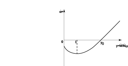
Figure 1: A schematic plot of $\dot{\omega}^{*}$ as a function of $y$ [Eq. (50)]. In fact, as $y\to 0$, $\omega^{*}$ approaches some negative $\dot{\omega}^{*}$, since the neutron star enters the propeller regime at small accretion rates.

Let us then vary Eq. (50) with respect to $y$:

$$I(\delta\dot{\omega}^{*})=I\frac{\partial\dot{\omega}^{*}}{\partial y}(\delta y)=\frac{3+2n}{11}A\dot{M}_{cr}^{\frac{3+2n}{11}}y^{-\frac{8-2n}{11}}\left(1-\frac{1}{y^{\frac{2n-1}{11}}}\right)(\delta y)\,.$$ (52)

We see that depending on whether $y>1$ or $y<1$, correlated changes of $\delta\dot{\omega}^{*}$ with X-ray flux should have different signs. Indeed, for GX 1+4 in González-Galán et al (2011) a positive correlation of the observed $\delta P$ with $\delta\dot{M}$ was found using Fermi data. This means that there is a negative correlation between $\delta\omega^{*}$ and $\delta\dot{M}$, suggesting $y<1$ in this source.

5 Determination of the neutron star magnetic field and other parameters in the settling accretion regime

Most X-ray pulsars rotate close to their equilibrium periods, i.e. the average $\dot{\omega}^{*}=0$. Near the equilibrium, in the settling accretion regime from Eq. (45) we obtain:

$$\mu_{30}^{(eq)}\approx\left[\frac{0.0986\cdot(0.034)^{(2-n)}\tilde{\omega}(1+(5/3)m_{t}^{2})}{1-z/Z}\right]^{\frac{11}{6n}}\left(\frac{P_{*}/100s}{P_{b}/10d}\right)^{\frac{11}{6n}}\left(\frac{\dot{M}_{16}(1+(5/3)m_{t}^{2})\psi(5/3,m_{t})}{\zeta}\right)^{\frac{1}{3}}\left(\frac{\sqrt{\delta}}{v_{8}}\right)^{\frac{11}{3}}$$ (53)

Once the magnetic field of the neutron star is estimated for any specific system, we can calculate the value of the Alfven radius $R_{A}$ [Eq. (43)] and the important numerical coefficient $f(u)$ [Eq. (44)]. The coupling constant $K_{1}(\theta)$ is evaluated from Eq. (46), in which the left-hand side can be independently calculated using Eq. (52) measured at $y=y_{0}$ (where $\dot{\omega}^{*}=0$):

$$A=\frac{I\left.\left(\frac{\partial\dot{\omega}^{*}}{\partial y}\right)\right|_{y_{0}}}{\left(\frac{3+2n}{11}\right)\frac{\dot{M}^{\frac{3+2n}{11}}}{y_{0}}\left(1-y_{0}^{\frac{-(2n-1)}{11}}\right)}\,.$$ (54)

The coefficient $Z$ is then determined from Eq. (26). The dimensionless factor relating the toroidal and poloidal magnetic field is also important. Near the equilibrium we have $\omega_{m}-\omega^{*}=-(z/Z)\omega^{*}$, so Eq. (23) can be written as

$$\frac{B_{t}}{B_{p}}=K_{1}(\theta)\left(\frac{z}{Z}\right)\left(\frac{\omega^{*}}{\omega_{K}(R_{A})}\right)=\frac{10f(u)z}{\sqrt{2}(1+(5/3)m_{t}^{2})\psi(5/3,m_{t})}\left(\frac{\omega^{*}}{\omega_{K}(R_{A})}\right)\,.$$ (55)

Calculated values for all parameters and coefficients discussed above are listed for specific wind-fed pulsars in Table 1 below.

5.1 Low-luminosity X-ray pulsars with torque reversal

Let us consider X-ray pulsars with persistent spin-up and spin-down episodes. We shall assume that a convective shell is present during both spin-up (with higher luminosity) and spin-down (with lower luminosity), provided that at the spin-up stage the mass accretion rate does not exceed $\dot{M}_{*}$ as derived above.

Suppose that in such pulsars we can measure the average value of $\dot{\omega}^{*}|_{su}$ and $\dot{\omega}^{*}|_{sd}$ as well as the average X-ray flux during spin-up and spin-down, respectively.

Let at some specific value $y_{1}<y_{0}$ the source be observed to spin-down:

$$I\dot{\omega}^{*}|_{sd}=A\dot{M}_{cr}^{\frac{3+2n}{11}}y_{1}^{\frac{3+2n}{11}}\left(1-\left(\frac{y_{0}}{y_{1}}\right)^{2n/11}\right)>0\,,\quad y_{1}<y_{0}=\left(\frac{3+2n}{3}\right)^{\frac{11}{2n}}\,.$$ (56)

At some $y_{2}>y_{0}$, the neutron star starts to spin-up:

$$I\dot{\omega}^{*}|_{su}=A\dot{M}_{cr}^{\frac{3+2n}{11}}y_{2}^{\frac{3+2n}{11}}\left(1-\left(\frac{y_{0}}{y_{2}}\right)^{2n/11}\right)<0\,,\quad y_{2}>y_{0}$$ (57)

Using the observed spin-down/spin-up ratio $\dot{\omega}^{*}|_{sd}/\dot{\omega}^{*}|_{su}=X$ and the corresponding X-ray luminosity ratio $L_{x}(sd)/L_{x}(su)=y_{1}/y_{2}=x<1$, we find by dividing Eq. (56) with Eq. (57) and after substituting $y_{2}=y_{1}/x$

$$|X|=x^{\frac{3+2n}{11}}\left|\frac{1-\left(\frac{y_{0}}{y_{1}}\right)^{2n/11}}{1-\left(\frac{y_{0}}{(y_{1}/x)}\right)^{2n/11}}\right|\,.$$ (58)

Solving this equation, we obtain $y_{1}$ and $y_{2}$ through the observed quantities $|X|$ and $x$. We stress that so far we have not used the absolute values of the X-ray luminosity (the mass accretion rate), only the ratio of the X-ray fluxes during spin-up and spin-down.

Here we should emphasize an important point. When the accretion rate through the shell exceeds some critical value $\dot{M}>\dot{M}^{*}$, the flow near the Alfven surface may become supersonic, a free-fall gap appears above the magnetosphere, and the angular momentum can not be removed from the magnetosphere. In that case the settling accretion regime is no longer realized, a shock is formed in the flow near the magnetosphere (the case studied by Burnard et al. 1982). Depending on the character of the inhomogeneities in the captured stellar wind, the specific angular momentum of the accreting matter can be prograde or retrograde, so alternating spin-up and spin-down episodes are possible. Thus the transition from the settling accretion regime (at low X-ray luminosities) to Bondi-Littleton accretion (at higher X-ray luminosities) can actually occur before $y$ reaches $y_{0}$. Indeed, by assuming a maximum possible value of the dimensioless velocity of matter settling $f(u)$=0.5 (for angular momentum removal from the magnetosphere to be possible, see Appendix D for more detail), we find from Eq. (44) :

$$\dot{M}^{*}_{16}\approx 3.7\left(\frac{\zeta}{(1+(5/3)m_{t}^{2})\psi(5/3,m_{t})}\right)^{1/12}\mu_{30}^{1/4}\,.$$ (59)

A similar estimate for the critical mass accretion rate for settling accretion can be obtained from a comparison of the characteristic Compton cooling time with the convective time at the Alfven radius.

6 Specific X-ray pulsars

In this Section, as an illustration of the possible applicability of our model to real sources, we consider three particular slowly rotating moderatly luminous X-ray pulsars: GX 301-2, Vela X-1, and GX 1+4. The first two pulsars are close to the equilibrium rotation of the neutron star, showing spin-up/spin-down excursions near the equilibrium frequency (apart from the spin-up/spin-down jumps, which may be, we think, due to episodic switch-ons of the strong coupling regime when the toroidal magnetic field component becomes comparable to the poloidal one, see Section 2.4.1). The third one, GX 1+4, is a typical example of a pulsar displaying long-term spin-up/spin-down episodes. During the last 30 years, it shows a steady spin-down with luminosity-(anti)correlated frequency fluctuations (see González-Galán et al. 2011 for a more detailed discussion). Clearly, this pulsar can not be considered to be in equilibrium.

6.1 GX 301-2

GX301–2 (also known as 4U1223–62) is a high-mass X-ray binary, consisting of a neutron star and an early type B optical companion with mass $\simeq 40M_{\odot}$ and radius $\simeq 60R_{\odot}$. The binary period is 41.5 days (Koh et al. 1997). The neutron star is a $\sim 680$ s X-ray pulsar (White et al. 1976), accreting from the strong wind of its companion ($\dot{M}_{loss}\sim 10^{-5}M_{\odot}$/yr, Kaper et al. 2006). The photospheric escape velocity of the wind is $v_{esc}\approx 500$ km/s. The semi-major axis of the binary system is $a\approx 170R_{\odot}$ and the orbital eccentricity $e\approx 0.46$. The wind terminal velocity was found by Kaper et al. (2006) to be about 300 km/s, smaller than the photospheric escape velocity.

GX 301-2 shows strong short-term pulse period variability, which, as in many other wind-accreting pulsars, can be well described by a random walk model (deKool & Anzer 1993). Earlier observations between 1975 and 1984 showed a period of $\sim 700$s while in 1984 the source started to spin up (Nagase 1989). BATSE observed two rapid spin-up episodes, each lasting about 30 days, and it was suggested that the long-term spin-up trend may have been due entirely to similar brief episodes as virtually no net changes in the frequency were found on long time-scales (Koh et al. 1997; Bildsten et al. 1997). The almost 10 years of spin-up were followed by a reversal of spin in 1993 (Pravdo & Ghosh 2001) after which the source has been continuously spinning down (La Barbera et al. 2005; Kreykenbohm et al. 2004, Doroshenko et al. 2010). Rapid spin-up episodes sometimes appear in the Fermi/GBM data on top of the long-term spin-down trend (Finger et al. 2011). It can not be excluded that these rapid spin-up episodes, as well as the ones observed in the BATSE data, reflect a temporary entrance into the strong coupling regime, as discussed in Section 2.4.1. Cyclotron line measurements (La Barbera et al. 2005) yield the magnetic field estimate near the neutron star surface $B_{0}\approx 4.4\times 10^{12}$ G ($\mu=1/2B_{0}R_{0}^{3}=2.2\times 10^{30}$ G cm³ for the assumed neutron star radius $R_{0}=10$ km).

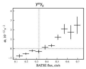
Figure 2: Torque-luminosity correlation in GX 301-2, $\dot{\omega}^{*}$ as a function of BATSE data (20-40 keV pulsed flux) near the equilibrium frequency, see Doroshenko et al. (2010). The assumed X-ray flux at equilibrium (in terms of the dimensionless parameter $y$) is also shown by the vertical dotted line.

In Fig. 2 we have plotted $\dot{\omega}^{*}$ as a function of the observed pulsed flux (20-40 keV) according to BATSE data (see Doroshenko et al. 2010 for more detail). To obtain the magnetic field estimate and other parameters (first of all, the coefficient $A$, see Eq. (54)) as described above in Section 5, we need to know the value of $\dot{M}$ and the derivative $\partial\dot{\omega}^{*}/\partial\dot{M}$ or $\partial\dot{\omega}^{*}/\partial y$. The estimate of $\dot{M}$ can be inferred from the X-ray flux provided the distance to the source is known, and generally this is a major uncertainty. We shall assume that near equilibrium a hot quasi-spherical shell exists in this pulsar, i.e. the accretion rate is $3\times 10^{16}$ g/s, i.e. not higher than the critical value $\dot{M}_{*}\simeq 4\times 10^{16}$ g/s [Eq. (59)]. While the absolute value of the mass accretion rate is necessary to estimate the magnetic field according to Eq. (53) (however, the dependence is rather weak, $\sim\dot{M}^{1/3}$), the derivative $\partial\dot{\omega}^{*}/\partial y$ can be derived from the $\dot{\omega}^{*}$ – X-ray flux plot, since in the first approximation the accretion rate is proportional to the observed pulsed X-ray flux. Near the equilibrium (the torque reversal point with $\dot{\omega}^{*}=0$), we find from a linear fit in Fig. 2 $\partial\dot{\omega}^{*}/\partial y\approx 4\times 10^{-13}$ rad/s².

The obtained parameters ($\mu$, $Z$, $K_{1}(theta)$, etc.) for this pulsar are listed in Table 1. We note that the magnetic field estimate resulting from our model for $n=2$ (boldfaced in Table 1) is fairly close to the value inferred from the cylcotron line measurements. We also note that for the case $n=3/2$ the coupling constants $Z$ and $K_{1}(\theta)$ turn out to be unrealistically large and the derived magentic field is very small, suggesting that assuming anisotropic turbulence is more realistic than using isotropic turbulence with the viscosity described by the Prandtl law.

6.2 Vela X-1

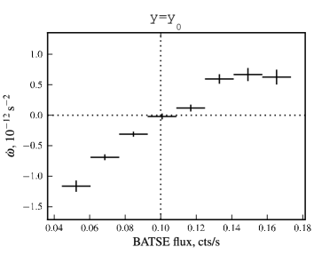
Figure 3: The same as in Fig. 2 for Vela X-1 (Doroshenko 2011, private communication).

Vela X-1 (=4U 0900-40) is the brightest persistent accretion-powered pulsar in the 20-50 keV energy band with an average luminosity of $L_{x}\approx 4\times 10^{36}$erg/s (Nagase 1989). It consists of a massive neutron star (1.88 $M_{\odot}$, Quaintrell et al. 2003) and the B0.5Ib super giant HD 77581, which eclipses the neutron star every orbital cycle of $\sim 8.964$ d (van Kerkwijk et al. 1995). The neutron star was discovered as an X-ray pulsar with a spin period of $\sim$283 s (Rappaport 1975), which has remained almost constant since the discovery of the source. The optical companion has a mass and radius of $\sim 23$ $M_{\odot}$ and $\sim 30$ $R_{sun}$ respectively (van Kerkwijk et al. 1995). The photospheric escape velocity is $v_{esc}\approx 540$ km/s. The orbital separation is $a\approx 50R_{\odot}$ and the orbital eccentricity $e\approx 0.1$. The primary almost fills its Roche lobe (as also evidenced by the presence of elliptical variations in the optical light curve, Bochkarev et al. (1975)). The mass-loss rate from the primary star is $10^{-6}$ $M_{\odot}$/yr (Nagase et al. 1986) via a fast wind with a terminal velocity of $\sim$ 1100 km/s (Watanabe et al. 2006), which is typical for this class. Despite the fact that the terminal velocity of the wind is rather large, the compactness of the system makes it impossible for the wind to reach this velocity before interacting with the neutron star, so the relative velocity of the wind with respect to neutron star is rather low, $\sim 700$ km/s.

Cyclotron line measurements (Staubert 2003) yields the magnetic field estimate $B_{0}\approx 3\times 10^{12}$ G ($\mu=1.5\times 10^{30}$ G cm³ for the assumed neutron star radius 10 km). We shall assume that in this pulsar $\dot{M}\simeq 3\times 10^{16}$ g/s (again for the existence of the shell to be possible). In Fig. 3 we have plotted $\dot{\omega}^{*}$ as a function of the observed pulsed flux (20-40 keV) according to BATSE data (Doroshenko 2011, private communication). As in the case of GX 301-2, from a linear fit we find at the spin-up/spin-down transition point $\partial\dot{\omega}^{*}/\partial y\approx 5.5\times 10^{-13}$ rad/s².

The obtained parameters for Vela X-1 are listed in Table 1. As in the case of GX 1+4, the magnetic field estimate given by our model for an almost iso-angular-momentum rotation law ($n=2$, boldfaced in Table 1) is close to the value inferred from the cyclotron line measurements.

6.3 GX 1+4

GX 1+4 was the first source to be identified as a symbiotic binary containing a neutron star (Davidsen, Malina & Bowyer 1977). The pulse period is $\sim 140$ s and the donor is an MIII giant (Davidsen et al. 1977). The system has an orbital period of 1161 days (Hinkle et al. 2006) making it the widest known LMXB by at least one order of magnitude. The donor is far from filling its Roche lobe and accretion onto the neutron star is by capture of the stellar wind of the companion.

The system has a very interesting spin history. During the 1970’s it was spinning up at the fastest rate ($\dot{\omega}_{su}\sim 3.8\cdot 10^{-11}$ rad/s) among the known X-ray pulsars at the time (e.g. Nagase 1989). After several years of non-detections in the early 1980’s, it reappeared again, now spinning down at a rate similar in magnitude to that of the previous spin-up. This spin-reversal has been interpreted in terms of a retrograde accretion disc forming in the system (Makishima et al. 1988, Dotani et al. 1989, Chakrabarty et al. 1997). A detailed spin-down history of the source is discussed in the recent paper by González-Galán et al. (2011). Using our model this behavior can, however, be readily explained by quasi-spherical accretion.

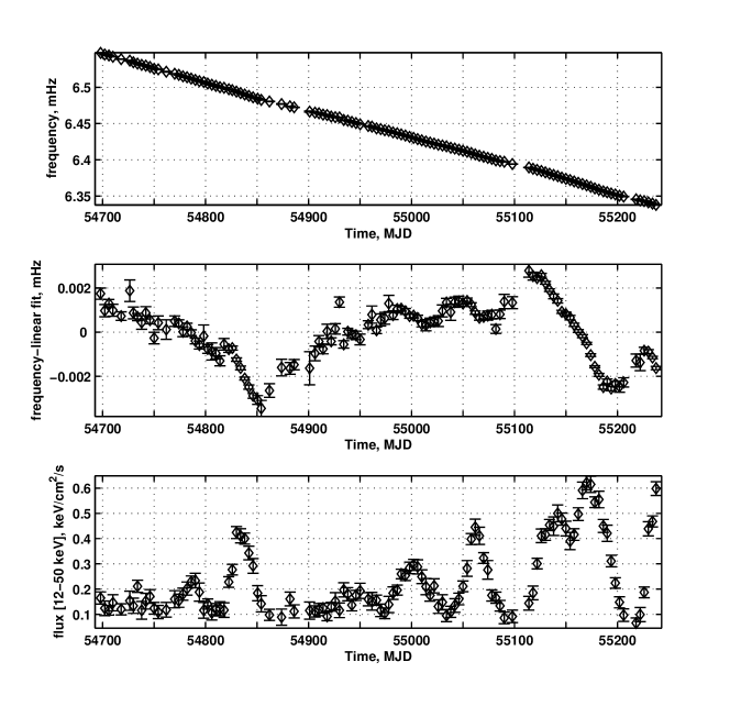
Figure 4: Pulsar frequency (upper panel), deviation of the frequency from the linear fit (middle panel) and pulsed flux in GX 1+4 from Fermi GBM data (M. Finger, private communication; see also González-Gálan et al (2011))

.

As the pulsar in GX 1+4 is not in equilibrium, we cannot directly use our method to estimate the magnetic field of the neutron star as described in Section 5. However, as GX 1+4 is currently experiencing a long-term spin-down trend, the first (spin-up) term in Eq. (45) must be smaller than the second (spin-down) term, which yields a lower limit on the value of the magnetic field (see Table 1).

Let us use Eq. (52) to quantitatively explain the observed anti-correlation between the pulsar frequency fluctuations and the X-ray flux, as observed in GX 1+4 (González-Galán et al., 2011). We use a fragment of four-day average Fermi/GBM data on GX 1+4 (M. Finger, private communication; see also González-Gálan et al (2011)). The pulsar is currently observed at the steady spin-down stage with a mean $\dot{\omega}_{sd}\approx-2.34\times 10^{-11}$ rad/s (the upper panel). In the middle panel of Fig. 4, deviations from the linear fit are shown. Note that the frequency excursions around the mean value is a few microseconds, while the pulsar frequency is much higher, a few milliseconds. This means that the frequency derivative is negative at all points within the time interval shown, i.e. no occasional spin-ups were observed, even at the highest X-ray flux levels.

Specifically, let us consider the prominent pulsar frequency change observed between MJD 55100 and MJD 55200 for around $\Delta t=80$ days. During this time period, the frequency of the pulsar decreased by $\Delta\omega^{*}\approx-3.6\times 10^{-5}$ rad (see Fig. 4). From here we find $\delta\dot{\omega}^{*}(obs)=\Delta\omega^{*}/\Delta t\approx-5.2\times 10^{-12}$ rad/s. Thus, the observed fractional change in the pulsar spin-down rate is $(\delta\dot{\omega}^{*}/|\dot{\omega}^{*}|)_{obs}\approx-0.2$.

On the other hand, by dividing Eq. (52) with Eq. (50) we find the expected relative fluctuations of $\dot{\omega}^{*}$ at a given mean accretion rate (or dimensionless X-ray luminosity $y$):

$$\frac{\delta\dot{\omega}^{*}}{|\dot{\omega}^{*}|}_{theor}=\frac{3+2n}{11}\frac{\delta\dot{M}}{\dot{M}}\left[\frac{1-y^{-\frac{2n-1}{11}}}{1-\left(\frac{y_{0}}{y}\right)^{\frac{2n}{11}}}\right]$$ (60)

From Fig. 4 (bottom panel) the range of the fluctuations relative to the mean value $(\delta\dot{M}/\dot{M})\simeq(0.6-0.2)/0.4\simeq 1$. Then, for the assumed $n=2$, the expected amplitude of the relative frequency derivative fluctuation would match the observed value if $y\simeq 0.2-0.3$. Important is that we find $y<1$, as must be the case for the observed negative sign of the torque-luminosity correlations.

Note here that the drop in flux-level during about 20 days at around MJD 55140-55160 should be translated to a decrease in $\dot{\omega}^{*}$, which is clearly seen in the upper panel of Fig. 4. A more detailed analysis using the entire Fermi data-set should be performed.

Further, note that the short-term spin-up episodes, sometimes observed on top of the steady spin-down behaviour (at about MJD 49700, see Fig. 2 in Chakrabarty et al. (1997)) are correlated with an enhancement of the X-ray flux, in contrast to the negative frequency-flux correlation discussed above. During these short spin-ups, $\dot{\omega}^{*}$ is about half the average $\dot{\omega}^{*}_{su}$ observed during the steady spin-up state of GX 1+4. The X-ray luminosity during these episodic spin-ups is approximately five times larger than the mean X-ray luminosity during the steady spin-down. We remind the reader that once $\dot{M}>\dot{M}_{*}$, a free-fall gap appears above the magnetosphere, and the neutron star can only spin up. When the X-ray flux drops again, the settling accretion regime is reestablished and the neutron star resumes its spinning-down.

Table 1: Parameters for the pulsars in Section 6. References for the observed spin periods, binary periods and spin down rate (for GX 1+4) are given in the text as well as discussions on the values used for the wind velocities with respect to the neutron star. The parameters Z, K${}_{1}(\Theta)$ and f(u) are defined in Section 2.4.2. Numerical estimates are given for dimensionless parameters $\delta=1,\zeta=1$, $\tilde{\omega}=1$, $\gamma=5/3$ and without turbulence ($m_{t}=0$). The numbers in boldface are the preferred values for a near iso-angular-momentum rotation law.

$$\begin{array}[]{lcccccc}\hline\cr Pulsar&\lx@intercol\hfil\rm GX301-2\hfil\lx@intercol&\lx@intercol\hfil\rm VelaX-1\hfil\lx@intercol&\lx@intercol\hfil\rm GX1+4\hfil\lx@intercol\\ \hline\cr\lx@intercol\hfil\hbox{Measured parameters}\hfil\lx@intercol\\ \hline\cr P_{*}{\rm(s)}&\lx@intercol\hfil 680\hfil\lx@intercol&\lx@intercol\hfil 283\hfil\lx@intercol&\lx@intercol\hfil 140\hfil\lx@intercol\\ P_{B}{\rm(d)}&\lx@intercol\hfil 41.5\hfil\lx@intercol&\lx@intercol\hfil 8.96\hfil\lx@intercol&\lx@intercol\hfil 1161\hfil\lx@intercol\\ v_{w}{\rm(km/s)}&\lx@intercol\hfil 300\hfil\lx@intercol&\lx@intercol\hfil 700\hfil\lx@intercol&\lx@intercol\hfil 200\hfil\lx@intercol\\ \frac{\partial\dot{\omega}}{\partial y}\arrowvert_{y_{0}}&\lx@intercol\hfil 4\cdot 10^{-13}\hfil\lx@intercol&\lx@intercol\hfil 5.5\cdot 10^{-13}\hfil\lx@intercol&\\ \dot{M}_{16}{\rm(\dot{M}/10^{16}})&\lx@intercol\hfil 3\hfil\lx@intercol&\lx@intercol\hfil 3\hfil\lx@intercol&\lx@intercol\hfil 1\hfil\lx@intercol\\ \hline\cr\lx@intercol\hfil\hbox{Derived parameters}\hfil\lx@intercol\\ \hline\cr&{\bf n=2}&n=3/2&{\bf n=2}&n=3/2&{\bf n=2}&n=3/2\\ \hline\cr\mu_{30}&{\bf 2.7}&0.1&{\bf 1.8}&0.16&{\bf>1.17}&>0.02\\ f(u)&{\bf 0.42}&0.57&{\bf 0.43}&0.54\\ K_{1}(\Theta)&{\bf 39}&3700&{\bf 36}&1150\\ Z&{\bf 13}&910&{\bf 12}&300\\ B_{t}/B_{p}&{\bf 0.1}&0.01&{\bf 0.2}&0.03\\ R_{A}{\rm(cm)}&{\bf 2\cdot 10^{9}}&3\cdot 10^{8}&{\bf 1.6\cdot 10^{9}}&4.2\cdot 10^{8}\\ \omega^{*}/\omega_{K}(R_{A})&{\bf 0.06}&0.004&{\bf 0.1}&0.01\\ \hline\cr\end{array}$$

7 Discussion

7.1 Physical conditions inside the shell

For an accretion shell to be formed around the neutron star magnetosphere it is necessary that the matter crossing the bow shock does not cool down too rapidly and thus starts to fall freely. This means that the radiation cooling time $t_{cool}$ must be longer than the characteristic time of plasma motion.

The plasma heats up in the strong shock to the temperature

$$T_{ps}=\frac{3}{16}\mu_{m}\frac{v_{w}^{2}}{\cal R}\approx 1.36\times 10^{5}[\hbox{K}]\left(\frac{v_{w}}{100\hbox{km/s}}\right)^{2}\,.$$ (61)

The radiative cooling time of the plasma is

$$t_{cool}=\frac{3kT}{2\mu_{m}n_{e}\Lambda}$$ (62)

where $\rho$ is the plasma density, $n_{e}=Y_{e}\rho/m_{p}$ is the electron number density ( $\mu_{m}=0.6$ and $Y_{e}\approx 0.8$ for fully ionized plasma with solar abundance); $\Lambda$ is the cooling function which can be approximated as

$$\Lambda(T)=\left\{\begin{array}[]{l}0,T<10^{4}\,{\rm K}\\ 1.0\times 10^{-24}T^{0.55},10^{4}\,{\rm K}<T<10^{5}\,{\rm K}\\ 6.2\times 10^{-19}T^{-0.6},10^{5}\,{\rm K}<T<4\times 10^{7}\,{\rm K}\\ 2.5\times 10^{-27}T^{0.5},T>4\times 10^{7}\,{\rm K}\end{array}\right.$$ (63)

(Raymond, Cox & Smith 1976; Cowie, McKee & Ostriker 1981).

Compton cooling becomes effective from the radius where the gas temperature $T$, determined by the hydrostatic formula Eq. (4), is lower than the X-ray Compton temperature $T_{x}$. The Compton cooling time (see Eq. (34)) is:

$$t_{C}\approx 1060[\hbox{s}]\dot{M}_{16}^{-1}\left(\frac{R}{10^{10}\hbox{cm}}\right)^{2}\,.$$ (64)

Above the radius where $T_{x}=T$, Compton heating dominates. Taking the actual temperature close to the adiabatic one [Eq. (4)], we find $R_{x}\approx 2\times 10^{10}$ cm. We note that both the Compton and photoionization heating processes are controlled by the photoionization parameter $\xi$ (Tarter et al. 1969, Hatchett et al. 1976)

$$\xi=\frac{L_{x}}{n_{e}R^{2}}\,.$$ (65)

In most part of the accretion flux, $n\sim R^{-3/2}$, so $\xi\sim R^{-1/2}$ and independent of the X-ray luminosity through the mass continuity equation. For characteristic values we find:

$$\xi\approx 5\times 10^{5}f(u)R_{10}^{-1/2}\,.$$ (66)

If Compton processes were effective everywhere, this high value of the parameter $\xi$ would imply that the plasma is Compton-heated up to keV-temperatures out to very large distances $\sim 10^{12}$ cm. However, at large distances the Compton heating time becomes longer than the characteristic time of gas accretion:

$$\frac{t_{C}}{t_{accr}}=\frac{t_{C}f(u)u_{ff}}{R}\approx 20f(u)\dot{M}_{16}^{-1}R_{10}^{1/2}\,,$$ (67)

which shows that Compton heating is ineffective. The gas temperature is determined by photoionization heating only and the gas can only be heated up to $T_{max}\approx 5\times 10^{5}$ K (Tarter et al. 1969), which is substantially lower than $T_{x}\sim 3$ keV. The sound velocity corresponding to $T_{max}$ is approximately 80 km/s.

The effective gravitational capture radius corresponding to the sound velocity of the gas in the photoionization-heated zone is

$$R_{B}^{*}=\frac{2GM}{c_{s}^{2}}=\frac{2GM}{\gamma{\cal R}T_{max}/\mu_{m}}\approx 3.5\times 10^{12}\hbox{cm}\left(\frac{T_{max}}{5\times 10^{5}\hbox{K}}\right)^{-1}\,.$$ (68)

Everywhere up to the bow shock photoionization keeps the temperature at a value $\simeq T_{max}$.

If the stellar wind velocity exceeds $80$ km/s, a standard bow shock is formed at the Bondi radius with a post-shock temperature given by Eq. (61). If the stellar wind velocity is lower than this value, the shock disappears and quasi-spherical accretion occurs from $R_{B}^{*}$.

The photoionization heating time at the effective Bondi radius $3\times 10^{12}$ cm is

$$t_{pi}\approx\frac{(3/2)kT_{max}/\mu_{m}}{(h\nu_{eff}-\zeta_{eff})n_{\gamma}\sigma_{eff}c}\approx 2\times 10^{4}[\hbox{s}]\dot{M}_{16}^{-1}\,.$$ (69)

(here $h\nu_{eff}\sim 10$ keV is the characteristic photon energy, $\zeta$ is the effective photoionization potential, $\sigma_{eff}\sim 10^{-24}$ cm² is the typical photoionization cross-section, $n_{\gamma}=L/(4\pi R^{2}h\nu_{eff}c)$ is the photon number density). The photoionization to accretion time ratio at the effective Bondi radius is then

$$\frac{t_{pi}}{t_{accr}}\approx 0.07f(u)\dot{M}_{16}^{-1}\,.$$ (70)

At wind velocities $v_{w}>80$ km/s the bow shock stands at the classical Bondi radius $R_{B}$ inside the effective Bondi radius $R_{B}^{*}$ determined by Eq. (68). The cooling time of the shocked plasma at $R_{B}$ expressed through the wind velocity $v_{w}$ is:

$$t_{cool}\approx 4.7\times 10^{4}[\hbox{s}]\dot{M}_{16}^{-1}v_{7}^{0.2}\,.$$ (71)

The photoionization heating time in the post-shock region can also be expressed through the stellar wind velocity:

$$t_{pi}\approx 3.5\times 10^{4}[\hbox{s}]\dot{M}_{16}^{-1}v_{7}^{-4}\,.$$ (72)

The comparison of these two timescales implies that at low velocities radiative cooling is important and the regime of free-fall accretion with conservation of specific angular momentum is realized.

So, at low wind velocities the plasma cools down and starts to fall freely. As the cold plasma approaches the gravitating center, photoionization heating becomes important and rapidly heats up the plasma to $T_{max}\approx 5\times 10^{5}$ K. Should this occur at a radius where $T_{max}<GM/({\cal R}R)$, the plasma continues its free fall down to the magnetosphere, still with the temperature $T_{max}$, with the subsequent formation of a shock above the magnetosphere. However, if $T_{max}$ is above the adiabatic temperatures at this radius, the settling accretion regime will be established even for low wind velocities.

For high-wind stellar velocities $v_{w}\gtrsim 100$ km/s, the post-shock temperature is higher than $T_{max}$, photoionization is unimportant, and the settling accretion regime is established if the radiation cooling time is longer than the accretion time. From a comparison of these timescales, we find the critical accretion rate as a function of of the wind velocity below which the settling accretion regime is possible:

$$\dot{M}_{16}^{**}\lesssim 0.12v_{7}^{3.2}\,.$$ (73)

Here we stress the difference of the critical acccretion rate $\dot{M}^{**}$ from $\dot{M}^{*}$ derived earlier. At $\dot{M}>\dot{M}^{**}$, the plasma rapidly cools down in the gravitational capture region and free-fall accretion begins (unless photoionization heats up the plasma above the adiabatic value at some radius), while at $\dot{M}>\dot{M}^{*}\simeq 4\times 10^{16}$ g/s determined by Eq. (59) a free-fall gap appears immediately above the neutron star magnetosphere.

7.2 On the possibility of the propeller regime

The very slow rotation of the neutron stars in GX 1+4, GX 301-2 and Vela X-1 ($\omega^{*}(R_{A})<\omega_{K}(R_{A})$) makes it hard to establish the propeller regime where matter is ejected with parabolic velocities from the magnetosphere during spin-down episodes.

Let us therefore start with estimating the important ratio of viscous tensions ($\sim B_{t}B_{p}$) to the gas pressure ($\sim B_{p}^{2}$) at the magnetospheric boundary. This ratio is proportional to $B_{t}/B_{p}$ (see Eq. (55)) and is always much smaller than 1 (see Table 1), i.e. only large-scale convective motions with the characteristic hierarchy of eddies scaled with radius can be established in the shell. When $\omega^{*}>\omega_{K}(R_{A})$, the propeller regime (without accretion) must set in. In that case the maximum possible braking torque is $\sim-\mu^{2}/R_{A}^{3}$ due to the strong coupling between the plasma and the magnetic field. Note that in the propeller state, interaction of the plasma with the magnetic field is in the strong coupling regime, i.e. where the toroidal magnetic field component $B_{t}$ is comparable to the poloidal one $B_{p}$. It can not be excluded that a hot iso-angular-momentum envelope could exist in this case as well, which would then remove angular momentum from the rotating magnetosphere. If the characteristic cooling time of the gas in the envelope is short in comparison to the falling time of matter, the shell disappears and one can expect the formation of a ‘storaging’ thin Keplerian disc around the neutron star magnetosphere (Sunyaev & Shakura 1977). There is no accretion of matter through such a disc. It only serves to remove angular momentum from the magnetosphere.

7.3 Effects of the hot shell on the X-ray energy and power spectrum

The spectra of X-ray pulsars are dominated by emission generated in the accretion column. The hot optically thin shell produces its own thermal emission, but even if all gravitational energy were released in the shell, the ratio of the X-ray luminosity from the shell to that of the accretion column would be about the ratio of the magnetosphere radius to the NS radius, i.e. one percent or less. In reality, it is much smaller. The shell should scatter X-ray radiation from the accretion column, but for this effect to be substantial, the Comptonization parameter $y$ must be of the order of one. The Thomson depth in the shell is, however, very small. Indeed, from the mass continuity equation and Eq. (43) for the Alfven radius and Eq. (44) for the factor $f(u)$, we get:

$$\tau_{T}=\int_{R_{A}}^{R_{B}}n_{e}(R)\sigma_{T}dR\approx 3.2\times 10^{-3}\dot{M}_{16}^{8/11}\mu_{30}^{-2/11}\,.$$

Therefore, for the temperature near the magnetosphere [Eq. (4)] the parameter $y$ is

$$y=\frac{4kT}{m_{e}c^{2}}\tau_{T}\approx 2.4\times 10^{-3}\,.$$

This means that the X-ray spectrum of the accretion column should not be significantly affected by scattering in the hot shell.

The large-scale convective motions in the shell introduce an intrinsic time-scale of the order of the free-fall time that could give rise to features (e.g. QPOs) in the power spectrum of variability. QPOs were reported in some X-ray pulsars (see Marykutty et al. 2010 and references therein). However, the expected frequency of the QPOs arising in our model would be of the order of mHz, much shorter than those reported.

A stronger effect can be the appearance of a dynamical instability of the shell on this time scale due to increased Compton cooling and hence increased mass accretion rate in the shell. This may result in a complete collapse of the shell resulting in an X-ray outburst with duration similar to the free-fall time scale of the shell ($\sim 1000$ s). Such a transient behaviour is observed in supergiant fast X-ray transients (SFXTs) (see Ducci et al. 2010). This interesting issue depends on the specific parameters of the shell and needs to be further investigated.

7.4 Can accretion discs (prograde or retrograde) be present in these pulsars?

The analysis of real pulsars carried out earlier suggested that in a convective shell an iso-angular-momentum distribution is the most plausible. Therefore, we shall below consider only this case, i.e. the rotation law $\omega\sim R^{-2}$. As follows from Eq. (29), at $\dot{\omega}^{*}=0$ the equilibrium angular frequency of the neutron star is

$$\omega^{*}_{eq}=\omega_{B}\frac{1}{1-z/Z}\left(\frac{R_{B}}{R_{A}}\right)^{2}\,.$$ (74)

We stress that such an equilibrium in our model is possible only when a shell is present. At high accretion rates $\dot{M}>\dot{M}_{*}\simeq 4\times 10^{16}$ g/s accretion proceeds in the free-fall regime (with no shell present).

Using Eq. (53), the equlibrium period for quasi-spherical settling accretion can be recasted to the form

$$P_{eq}\approx 1000[\hbox{s}]\mu_{30}^{12/11}\left(\frac{P_{b}}{10\hbox{d}}\right)\left(\frac{\zeta}{(1+(5/3)m_{t}^{2})\psi(5/3,m_{t})\dot{M}_{16}}\right)^{4/11}\left(\frac{v_{8}}{\sqrt{\delta}}\right)^{4}\frac{(1-z/Z)}{\tilde{\omega}(1+(5/3)m_{t}^{2})}\,.$$ (75)

For standard disc accretion, the equilibrium period is

$$P_{eq,d}\approx 7\hbox{s}\mu_{30}^{6/7}\dot{M}_{16}^{-3/7}\,,$$ (76)

and the long periods observed in some X-ray pulsars can be explained assuming a very high magnetic field of the neutron star. Retrograde accretion discs are also discussed in the literature (see, e.g., Nelson et al. (1997) and references therein). Torque reversals produced by prograde/retrograde discs can in principle lead to very long periods for X-ray pulsars even with standard magnetic fields. Retrograde discs can be formed due to inhomogeneities in the captured stellar wind (Ruffert 1997, 1999). This might be the case at high accretion rates when hot quasi-spherical shell cannot exist. In the case of GX 1+4, however, it is highly unlikely to observe a retrograde disk on a time scale much longer than the orbital period (see a more detailed discussion of this issue in Gozález-Galán et al. (2011)). In the case of GX 301-2 and Vela X-1, the observed positive torque-luminosity correlation (see Figs. 2 and 3) rules out a retrograde disc as well.

To conclude the discussion, we should mention that real systems (including those considered here) demonstrate a complex quasi-stationary behaviour with dips, outbursts, etc. These considerations are beyond the scope of this paper and definitely deserve further observational and theoretical studies.

8 Conclusions

In this paper we have presented a theoretical model for quasi-spherical subsonic accretion onto slowly rotating magnetized neutron stars. In this model the accreting matter is gravitationally captured from the stellar wind of the optical companion and subsonically settles down onto the rotating magnetosphere forming an extended quasi-static shell. This shell mediates the angular momentum removal from the rotating neutron star magnetosphere during spin-down states by large-scale convective motions. A detailed analysis and comparison with observations of two specific X-ray pulsars GX 301-2 and Vela X-1 demonstrating torque-luminosity correlations near the equilibrium neutron star spin period shows that most likely strongly anisotropic convective motions are established, with an almost iso-angular-momentum distribution of rotational velocities $\omega\sim R^{-2}$. A statistical analysis of long-period X-ray pulsars with Be-components in SMC (Chashkina & Popov 2011) also favored the rotation law $\omega\sim R^{-2}$. The accretion rate through the shell is determined by the ability of the plasma to enter the magnetosphere. The settling regime of accretion which allows angular momentum removal from the neutron star magnetosphere can be realized for moderate accretion rates $\dot{M}<\dot{M}_{*}\simeq 4\times 10^{16}$ g/s. At higher accretion rates a free-fall gap above the neutron star magnetosphere appears due to rapid Compton cooling, and accretion becomes highly non-stationary.

From observations of the spin-up/spin-down rates (the angular rotation frequency derivative $\dot{\omega}^{*}$, or $\partial\dot{\omega}^{*}/\partial\dot{M}$ near the torque reversal) of long-period X-ray pulsars with known orbital periods it is possible to determine the main dimensionless parameters of the model, as well as to estimate the magnetic field of the neutron star. Such an analysis revealed good agreement between the magnetic field estimates in the pulsars GX 301-2 and Vela X-1 obtained using our model and derived from the cyclotron line measurements.

In our model, long-term spin-up/spin-down as observed in some X-ray pulsars can be quantitatively explained by a change in the mean mass accretion rate onto the neutron star (and the corresponding mean X-ray luminosity). Clearly, these changes are related to the stellar wind properties.

The model also predicts the specific behaviour of the variations in $\delta\dot{\omega}^{*}$, observed on top of a steady spin-up or spin-down, as a function of mass accretion rate fluctuations $\delta\dot{M}$. There is a critical accretion rate $\dot{M}_{cr}$ below which an anti-correlation of $\delta\dot{\omega}^{*}$ with $\delta\dot{M}$ should occur (the case of GX 1+4 at the steady spin-down state currently observed), and above which $\delta\dot{\omega}^{*}$ should correlate with $\delta\dot{M}$ fluctuations (the case of Vela X-1, GX 301-2, and GX 1+4 in the steady spin-up state). The model explains quantitatively the relative amplitude and the sign of the observed frequency fluctuations in GX 1+4.

Appendix A The structure of a quasi-spehrical accreting rotating shell

A.1 Basic equations

Let us first write down the Navier-Stokes equations in spherical coordinates $R,\theta,\phi$. Due to the huge Reynolds numbers in the shell ($\sim 10^{15}-10^{16}$ for a typical accretion rate of $10^{17}$ g/s and magnetospheric radius $\sim 10^{8}$ cm), there must be turbulence. In this case the Navier-Stokes equations are usually called the Reynolds equations. In the general case, the turbulent viscosity can depend on the coordinates, so the equations take the form:

1. Mass continuity equation:

$$\frac{\partial\rho}{\partial t}+\frac{1}{R^{2}}\frac{\partial}{\partial R}\left(R^{2}\rho u_{R}\right)+\frac{1}{R\sin\theta}\frac{\partial}{\partial\theta}\left(\sin\theta\,\rho u_{\theta}\right)+\frac{1}{R\sin\theta}\frac{\partial\rho u_{\phi}}{\partial\phi}=0.$$ (77)

2. The $R$-component of the momentum equation:

$$\frac{\partial u_{R}}{\partial t}+u_{R}\displaystyle\frac{\partial u_{R}}{\partial R}+\displaystyle\frac{u_{\theta}}{R}\displaystyle\frac{\partial u_{R}}{\partial\theta}+\displaystyle\frac{u_{\phi}}{R\sin\theta}\displaystyle\frac{\partial u_{R}}{\partial\phi}-\displaystyle\frac{u_{\phi}^{2}+u_{\theta}^{2}}{R}=-\displaystyle\frac{GM}{R^{2}}+N_{R}$$ (78)

3. The $\theta$-component of the momentum equation:

$$\frac{\partial u_{\theta}}{\partial t}+u_{R}\displaystyle\frac{\partial u_{\theta}}{\partial R}+\displaystyle\frac{u_{\theta}}{R}\displaystyle\frac{\partial u_{\theta}}{\partial\theta}+\displaystyle\frac{u_{\phi}}{R\sin\theta}\displaystyle\frac{\partial u_{\theta}}{\partial\phi}+\displaystyle\frac{u_{R}u_{\theta}-u_{\phi}^{2}\cot\theta}{R}=N_{\theta}$$ (79)

4. The $\phi$-component of the momentum equation:

$$\frac{\partial u_{\phi}}{\partial t}+u_{R}\displaystyle\frac{\partial u_{\phi}}{\partial R}+\displaystyle\frac{u_{\theta}}{R}\displaystyle\frac{\partial u_{\phi}}{\partial\theta}+\displaystyle\frac{u_{\phi}}{R\sin\theta}\displaystyle\frac{\partial u_{\phi}}{\partial\phi}+\displaystyle\frac{u_{R}u_{\phi}+u_{\phi}u_{\theta}\cot\theta}{R}=N_{\phi}$$ (80)

Here the force components (including viscous force and gas pressure gradients) read:

$$\rho N_{R}=\frac{1}{R^{2}}\frac{\partial}{\partial R}\left(R^{2}W_{RR}\right)+\frac{1}{\sin\theta\,R}\frac{\partial}{\partial\theta}\left(W_{R\theta}\sin\theta\right)+\frac{1}{\sin\theta\,R}\frac{\partial}{\partial\phi}W_{R\phi}-\frac{W_{\theta\theta}}{R}-\frac{W_{\phi\phi}}{R}$$ (81)

$$\rho N_{\theta}=\frac{1}{R^{2}}\frac{\partial}{\partial R}\left(R^{2}W_{\theta R}\right)+\frac{1}{\sin\theta\,R}\frac{\partial}{\partial\theta}\left(W_{\theta\theta}\sin\theta\right)+\frac{1}{\sin\theta\,R}\frac{\partial}{\partial\phi}W_{\theta\phi}-\cot\theta\frac{W_{\theta\theta}}{R}$$ (82)

$$\rho N_{\phi}=\frac{1}{R^{3}}\frac{\partial}{\partial R}\left(R^{3}W_{\phi R}\right)+\frac{1}{\sin\theta\,R}\frac{\partial}{\partial\theta}\left(W_{\phi\theta}\sin\theta\right)+\frac{1}{\sin\theta\,R}\frac{\partial}{\partial\phi}W_{\phi\phi}$$ (83)

The components of the stress tensor include a contribution from both the gas pressure $P_{g}$ (assumed to be isotropic) and the turbulent pressure $P^{t}$ (generally anisotropic). In their definition we shall follow the classical treatment by Landau and Lifshitz (1986), but with the inclusion of anisotropic turbulent pressure:

$$W_{RR}=-P_{g}-P_{RR}^{t}+2\rho\nu_{t}\frac{\partial u_{R}}{\partial R}-\frac{2}{3}\rho\nu_{t}{\rm div}{\bf u}$$ (84)

$$W_{\theta\theta}=-P_{g}-P_{\theta\theta}^{t}+2\rho\nu_{t}\left(\frac{1}{R}\frac{\partial u_{\theta}}{\partial\theta}+\frac{u_{R}}{R}\right)-\frac{2}{3}\rho\nu_{t}{\rm div}{\bf u}$$ (85)

$$W_{\phi\phi}=-P_{g}-P_{\phi\phi}^{t}+2\rho\nu_{t}\left(\frac{1}{R\sin\theta}\frac{\partial u_{\phi}}{\partial\phi}+\frac{u_{R}}{R}+\frac{u_{\theta}\cot\theta}{R}\right)-\frac{2}{3}\rho\nu_{t}{\rm div}{\bf u}$$ (86)

$$W_{R\theta}=\rho\nu_{t}\left(\frac{1}{R}\frac{\partial u_{R}}{\partial\theta}+\frac{\partial u_{\theta}}{\partial R}-\frac{u_{\theta}}{R}\right)$$ (87)

$$W_{\theta\phi}=\rho\nu_{t}\left(\frac{1}{R\sin\theta}\frac{\partial u_{\theta}}{\partial\phi}+\frac{1}{R}\frac{\partial u_{\phi}}{\partial\theta}-\frac{u_{\phi}\cot\theta}{R}\right)$$ (88)

$$W_{R\phi}=\rho\nu_{t}\left(\frac{1}{R\sin\theta}\frac{\partial u_{R}}{\partial\phi}+\frac{\partial u_{\phi}}{\partial R}-\frac{u_{\phi}}{R}\right)$$ (89)

In our problem the anistropy of the turbulence is such that $P_{RR}^{t}=P_{\parallel}^{t}$, $P_{\theta\theta}^{t}=P_{\phi\phi}^{t}=P_{\perp}^{t}$. The turbulent pressure components can be expressed through turbulent Mach numbers and will be given in Appendix D.

${\rm div}{\bf u}$ in spherical coordinates is:

$${\rm div}{\bf u}=\frac{1}{R^{2}}\frac{\partial}{\partial R}\left(R^{2}u_{R}\right)+\frac{1}{R\sin\theta}\frac{\partial}{\partial\theta}\left(\sin\theta\,u_{\theta}\right)+\frac{1}{R\sin\theta}\frac{\partial u_{\phi}}{\partial\phi}.$$ (90)

A.2 Symmetries of the problem

We shall consider axially-symmetric ($\displaystyle\frac{\partial}{\partial\phi}=0$), stationary ($\displaystyle\frac{\partial}{\partial t}=0$), and only radial accretion ($u_{\theta}=0$). Under these conditions, from the continuity equation Eq. (77) we obtain:

$$\dot{M}=4\pi R^{2}\rho u_{R}=const\,.$$ (91)

The constant here is determined from the condition of plasma leakage through the magnetosphere.

Let us rewrite the Reynolds equations under the above assumptions. The $R$-component of the momentum Eq. (78) equation becomes:

$$\rho\left(u_{R}\displaystyle\frac{\partial u_{R}}{\partial R}-\displaystyle\frac{u_{\phi}^{2}}{R}\right)=-\rho\displaystyle\frac{GM}{R^{2}}+\frac{1}{R^{2}}\frac{\partial}{\partial R}\left(R^{2}W_{RR}\right)+\frac{1}{\sin\theta\,R}\frac{\partial}{\partial\theta}\left(W_{R\theta}\sin\theta\right)-\frac{W_{\theta\theta}}{R}-\frac{W_{\phi\phi}}{R}$$ (92)

The $\theta$-component of the momentum equation:

$$-\rho\frac{u_{\phi}^{2}\cot\theta}{R}=\frac{1}{R^{2}}\frac{\partial}{\partial R}\left(R^{2}W_{\theta R}\right)+\frac{1}{\sin\theta\,R}\frac{\partial}{\partial\theta}\left(W_{\theta\theta}\sin\theta\right)-\cot\theta\frac{W_{\theta\theta}}{R}$$ (93)

The $\phi$-component of the momentum equation:

$$\rho\left(u_{R}\displaystyle\frac{\partial u_{\phi}}{\partial R}+\displaystyle\frac{u_{R}u_{\phi}}{R}\right)=\frac{1}{R^{3}}\frac{\partial}{\partial R}\left(R^{3}W_{\phi R}\right)+\frac{1}{\sin\theta\,R}\frac{\partial}{\partial\theta}\left(W_{\phi\theta}\sin\theta\right)$$ (94)

The components of the stress tensor with anisotropic turbulence take the form:

$$W_{RR}=-P_{g}-P_{\parallel}^{t}-\frac{4}{3}\rho\nu_{t}\left(\frac{u_{R}}{R}-\frac{\partial u_{R}}{\partial R}\right)$$ (95)

$$W_{\theta\theta}=-P_{g}-P_{\perp}^{t}+\frac{2}{3}\rho\nu_{t}\left(\frac{u_{R}}{R}-\frac{\partial u_{R}}{\partial R}\right)$$ (96)

$$W_{\phi\phi}=-P_{g}-P_{\perp}^{t}+\frac{2}{3}\rho\nu_{t}\left(\frac{u_{R}}{R}-\frac{\partial u_{R}}{\partial R}\right)$$ (97)

$$W_{R\theta}=\rho\nu_{t}\frac{1}{R}\frac{\partial u_{R}}{\partial\theta}$$ (98)

$$W_{\theta\phi}=\rho\nu_{t}\left(\frac{1}{R}\frac{\partial u_{\phi}}{\partial\theta}-\frac{u_{\phi}\cot\theta}{R}\right)$$ (99)

$$W_{R\phi}=\rho\nu_{t}\left(\frac{\partial u_{\phi}}{\partial R}-\frac{u_{\phi}}{R}\right)$$ (100)

Generally, there are two separate cases – with isotropic turbulence and anisotropic turbulence, which shall be treated differently. First we consider the simplest case of isotropic turbulence with Prandtl law for turbulent viscosity. The more general case of anisotropic turbulence will be discussed separately in Appendix B.

A.3 Viscosity prescription for isotropic turbulence

We consider an axisymmetric flow with a very large Reynolds number. By generalizing the Prandtl law for the turbulent velocity obtained for plane parallel flows, the turbulent velocity scales as $u_{t}\sim l_{t}R(\partial\omega/\partial R)$. From the similarity laws of gas-dynamics we assume $l_{t}\sim R$, so

$$u_{t}=C_{1}R^{2}\left|\frac{\partial\omega}{\partial R}\right|\,.$$ (101)

We note that in our case the turbulent velocity is determined by convection, so $u_{t}\lesssim 0.5u_{ff}$ (see Appendix D). This implies that the constant $C_{1}$ scales as

$$C_{1}\sim u_{t}/\langle u_{\phi}\rangle,$$ (102)

and can be very large since $\langle u_{\phi}\rangle\ll u_{t}$. So the turbulent viscosity coefficient reads:

$$\nu_{t}=\langle u_{t}l_{t}\rangle=C_{2}C_{1}R^{3}\left|\frac{\partial\omega}{\partial R}\right|$$ (103)

Here $C_{2}\approx 1/3$ is a numerical factor originating from statistical averaging. Below we shall combine $C_{1}$ and $C_{2}$ into the new coefficient $C=C_{1}C_{2}$, which can be much larger than one. Due to interaction of convection cells in the sheared flux the amplitude of turbulent motions is thus much larger than the average rotation velocity.

A.4 The angular momentum transport equation and the rotation law inside the shell

A similar problem (that of a rotating sphere in a viscous fluid) was solved in Landau and Lifshitz (1986). It was found that the variables are separated and $u_{\phi}(R,\theta)=U_{\phi}(R)\sin\theta$. Note that the angular velocity $\omega(R)=U_{\phi}(R)/R$ is independent of $\theta$. Our problem is different from that of the sphere in a viscous fluid in several respects: 1) there is a force of gravity present, 2) the turbulent viscosity varies with $R$ and can in principle depend on $\theta$, and 3) there is radial motion of matter (accretion). These differences lead, as will be shown below, to the radial dependence $U_{\phi}(R)\propto R^{-1/2}$. (We recall that for a rotating sphere in a viscous fluid $U_{\phi}\propto R^{-2}$).

Let us start with solving Eq. (94). First, we note that for $u_{\phi}(\theta)\sim\sin\theta$, according to Eq. (99), $W_{\theta\phi}=0$. Next, making use of the continuity equation Eq. (153) and the definition of angular velocity, we rewrite Eq. (94) in the form of angular momentum transfer by viscous forces:

$$\frac{\dot{M}}{R}\frac{\partial}{\partial R}\omega R^{2}=\frac{4\pi}{R}\frac{\partial}{\partial R}R^{3}W_{R\phi}$$ (104)

Now we can integrate Eq. (104) with respect to $R$ to get

$$\dot{M}\omega R^{2}=4\pi R^{3}W_{R\phi}+D\,,$$ (105)

where $D$ is an integration constant. In the case of isotropic turbulence, the viscous stress component (force per unit area) from Eq. (100) is

$$W_{R\phi}=\rho\nu_{t}R\frac{\partial\omega}{\partial R}$$ (106)

so we obtain

$$\dot{M}\omega R^{2}=4\pi\rho\nu_{t}R^{4}\frac{\partial\omega}{\partial R}+D\,.$$ (107)

This equation for angular mometum transport by turbulent viscosity is similar to that for disc accretion (Shakura and Sunyaev 1973), but different due to spherical symmetry of the problem under consideration.

The left part of Eq. (107) is simply advection of specific angular momentum averaged over the sphere ($1/2\int_{0}^{\pi}\omega R^{2}\sin^{2}\theta\sin\theta d\theta=1/3\omega R^{2}$) by the average motion toward the gravitational center (accretion). $\dot{M}$ is negative as well as $\frac{\partial\omega}{\partial R}$. The first term on the right describes transport of angular momentum outwards by turbulent viscous forces.

The constant $D$ is determined from the equation

$$D=K_{1}(\theta)K_{2}\frac{\mu^{2}}{R_{A}^{3}}\frac{\omega_{m}-\omega^{*}}{\omega_{K}(R_{A})}$$ (108)

(see Eq. (24) in the text). We consider accretion onto a magnetized neutron star. When $D<0$, the advection term in the left part of Eq. (107) dominates over viscous angular momentum transfer outwards. Oppositely, when $D>0$, the viscous term in the right part of Eq. (107) dominates. In the case of $\dot{M}=0$ (no plasma enters the magnetosphere), there is only angular momentum transport outwards by viscous forces.

Now let us rewrite Eq. (108) in the form

$$D=K_{1}(\theta)K_{2}\frac{\mu^{2}}{R_{A}^{6}}R_{A}^{3}\frac{\omega_{m}-\omega^{*}}{\omega_{K}(R_{A})}$$ (109)

and use the pressure balance condition

$$P(R_{A})=P_{g}(R_{A})(1+\gamma m_{t}^{2})=\frac{B^{2}(R_{A})}{8\pi}=\frac{K_{2}}{2\pi}\frac{\mu^{2}}{R_{A}^{6}}\,.$$ (110)

Using the mass conitnuity equation in the form

$$|\dot{M}|=4\pi R^{2}\rho f(u)\sqrt{GM/R}\,,$$

and the expression for the gas pressure Eq. (8), we write the integration constant $D/|\dot{M}|$ in the form

$$\frac{D}{|\dot{M}|}=K_{1}\frac{(\gamma-1)}{\gamma}\psi(\gamma,m_{t})\frac{(\omega_{m}-\omega^{*})R_{A}^{2}}{2\sqrt{2}f(u)}(1+\gamma m_{t}^{2})\,.$$ (111)

Let us consider the case near the neutron star rotation equilibrium $\dot{\omega}^{*}=0$. In this case according to Eq. (27)

$$\omega_{m}-\omega^{*}=-\frac{z}{Z}\omega^{*}\,,$$ (112)

so using definition $Z$ [Eq. (26)], we obtain:

$$\frac{D}{|\dot{M}|}=-zR_{A}^{2}\omega^{*}\,.$$ (113)

We emphasize that the value of the constant $D$ is fully determined by the dimensionless specific angular momentum of matter at the Alfven radius $z$.

A.5 Angular rotation law

Let us use Eq. (107) to find the rotation law $\omega(R)$. At large distances $R\gg R_{A}$ (we remind the reader that $R_{A}$ is the bottom radius of the shell) the constant $D$ is small relative to the other terms, so we can set $D\approx 0$. Thus, to obtain the rotation law we shall neglect this constant in the right part of Eq. (107). Next, we substitute Eq. (103) and make use of the solution for the density (which, as we shall show below, remains the same as in the hydrostatic solution)

$$\rho(R)=\rho(R_{A})\left(\frac{R_{A}}{R}\right)^{3/2}\,$$ (114)

in Eq. (107) to obtain

$$\left|\dot{M}\right|\omega R^{2}=4\pi\rho(R_{A})\left(\frac{R_{A}}{R}\right)^{3/2}CR^{7}\left(\frac{\partial\omega}{\partial R}\right)^{2}\,.$$ (115)

After integrating this equation, we find

$$2\omega^{1/2}=\pm\frac{4}{3}\frac{K^{1/2}}{R^{3/4}}+D_{1}$$ (116)

where

$$K=\frac{|\dot{M}|}{4\pi\rho(R_{A})CR_{A}^{3/2}}$$ (117)

and $D_{1}$ is some integration constant. In Eq. (116) we use only the positive solution (the minus sign with constant $D_{1}>0$ would correspond to a solution with the angular velocity growing outwards, which is possible if the pulsar rotation is zero). If $D_{1}\neq 0$, at large $R\gg R_{A}$ (in the zone close to the bow shock) the solid body rotation law would lead to $\omega\to const\approx\omega_{B}$. (However, we remind the reader that our discussion is not applicable close to the bow shock region.) At small distances from the Alfvenic surface the effect of this constant is small and we shall neglect it in the calculations below. Then we find

$$\omega(R)=\frac{4}{9}\frac{|\dot{M}|}{4\pi\rho(R_{A})CR_{A}^{3}}\left(\frac{R_{A}}{R}\right)^{3/2}$$ (118)

i.e. the quasi-Keplerian law $\omega(R)=\omega_{m}(R_{A}/R)^{3/2}$. The constant $\omega_{m}$ in the solution given by Eq. (118) is obtained after substituting $\dot{M}$ from the continuity equation at $R=R_{A}$ into Eq. (118):

$$\omega_{m}\equiv\tilde{\omega}\omega(R_{A})=\frac{4}{9}\tilde{\omega}\frac{|u_{R}(R_{A})|}{CR_{A}}\,.$$ (119)

(Here we have introduced the correction factor $\tilde{\omega}>1$ to account for the deviation of the exact solution from the Keplerian law near $R_{A}$).

As $u_{R}(R_{A})$ is smaller than the free-fall velocity, the above formula implies that $\omega_{m}<\omega_{K}(R_{A})$, lower than the Keplerian angular frequency. For self-consistency the coefficient $C$ in the Prandtl law is determined, according to Eq. (119), by the ratio of the radial velocity $u_{R}$ to the rotational velocity of matter $U_{\phi}$:

$$C=\frac{4}{9}\tilde{\omega}\frac{|u_{R}(R_{A})|}{\omega_{m}R_{A}}=\frac{4}{9}\tilde{\omega}\frac{|u_{R}(R_{A})|}{U_{\phi}(R_{A})}\,.$$ (120)

Note that this ratio is independent of the radius $R$ and is actually constant across the shell. Indeed, the radial dependence of the velocity $u_{R}$ follows from the continuity equation with account for the density distribution Eq. (114)

$$u_{R}(R)=u_{R}(R_{A})\left(\frac{R_{A}}{R}\right)^{1/2}\,.$$ (121)

For the quasi-Keplerian law $u_{\phi}(R)\sim 1/R^{1/2}$, so the ratio $u_{R}/U_{\phi}$ is constant. Finally, the angular frequency of the shell rotation near the magnetosphere $\omega_{m}$ is related to the angular frequency of the motion of matter near the bow-shock as

$$\omega_{m}=\tilde{\omega}\omega_{B}\left(\frac{R_{B}}{R_{A}}\right)^{3/2}$$ (122)

In fact, when approaching $R_{A}$, the integration constant $D$ (which we neglected at large distances $R\gg R_{A}$) should be taken into account. The rotational law will thus be different from the Keplerian one.

We stress the principal difference between this regime of accretion and disc accretion. For disc accretion the radial velocity is much smaller than the turbulent velocity, and the tangential velocity is almost Keplerian and is much larger than the turbulent velocity. The radial velocity in the quasi-spherical case is not determined by the rate of the angular momentum removal. It is determined only by the ”permeability” of the neutron star magnetosphere for infalling matter. In our case we assumed it to be of the order of the convection velocity. The tangential velocity for the obtained quasi-Keplerian law is much smaller than the velocity of convective motions in the shell. Note also that in the case of disc accretion the turbulence can be parametrized by only one dimensionless parameter $\alpha\approx u_{t}^{2}/u_{s}^{2}$ with $0<\alpha<1$ (Shakura & Sunyaev 1973). The matter in an accretion disc differentially rotates with a supersonic (almost Keplerian) velocity, while in our case the shell rotates differentially with a substantially subsonic velocity at any radius, and the turbulence in the shell is essentially subsonic. Of course, our case with an extended shell is strongly different from the regime of freely falling matter with a standing shock above the magnetosphere (Arons & Lea 1976a).

A.6 The case without accretion

Now let us consider the case when the plasma can not enter the magnetosphere and no accretion onto the neutron star occurs. This case is similar to the subsonic propeller regime considered by Davies and Pringle (1981). Eq. (107) then takes the form:

$$0=4\pi\rho\nu_{t}R^{4}\frac{\partial\omega}{\partial R}+D\,.$$ (123)

(We remind the reader that the constant $D$ is determined by the spin-down rate of the neutron star, $D=I\dot{\omega}^{*}<0$). Solving this equation as above, we find for the rotation law in this case:

$$\omega(R)=\omega_{m}\left(\frac{R_{A}}{R}\right)^{7/4}\,,$$ (124)

where

$$\omega_{m}=\frac{I|\dot{\omega}^{*}|}{7\pi\rho(R_{A})\nu_{t}(R_{A})R_{A}^{3}}\,.$$ (125)

From Eq. (103) we find

$$\nu_{t}(R_{A})=\frac{7}{4}C\omega_{m}R_{A}^{2}\,,$$ (126)

so for $\omega_{m}$ we obtain:

$$\omega_{m}=\frac{2}{7}\left(\frac{I|\dot{\omega}^{*}|}{\pi C\rho(R_{A})R_{A}^{5}}\right)^{1/2}\,.$$ (127)

On the other hand, $\omega_{m}$ is now related to the bow-shock region parameters as

$$\omega_{m}=\omega_{B}\left(\frac{R_{B}}{R_{A}}\right)^{7/4}\,.$$ (128)

Appendix B The case with anisotropic turbulence

The Prandl rule for viscosity used above that relates the scale and velocity of turbulent pulsations with the average angular velocity is commonly used when the turbulence is generated by the shear itself. In our problem, the turbulence is initiated by large-scale convective motions in the gravitational field. During convection, a strong anisotropic turbulent motions can appear (the radial dispersion of chaotic motions could be much larger than the dispersion in the tangential direction), and the Prandl law could be inapplicable. Anisotropic turbulence is much more complicated and remains a poorly studied case.

As a first step, we can adopt the empirical law for $W_{R\phi}$ suggested by Wasiutinski (1946):

$$W_{R\phi}=2\rho(-\nu_{t}+\nu_{r})\omega+\nu_{r}\rho R\frac{d\omega}{dR}$$ (129)

where the radial and tangential kinematic viscosity coefficients are

$$\nu_{r}=C_{\parallel}\langle|u_{\parallel}^{t}|\rangle R$$

$$\nu_{t}=C_{\perp}\langle|u_{\perp}^{t}|\rangle R$$

respectively. Dimensiionless constants $C_{\parallel}$ and $C_{\perp}$ are of the order of one. In the isotropic case, $\nu_{r}=\nu_{t}$, $W_{R\phi}\sim d\omega/dR$, and in the strongly anisotropic case, $\nu_{r}\gg\nu_{t}$, $W_{R\phi}\sim d(\omega R^{2})/dR$. Using these definitions, let us substitute Eq. (129) in Eq. (105) and rewrite the latter in the form:

$$\omega R^{2}\left(1-\frac{2C_{\perp}\langle|u_{\perp}^{t}|\rangle}{|u_{R}|}\right)=C_{\parallel}\frac{\langle|u_{\parallel}^{t}|\rangle}{|u_{R}|}\frac{Rd(\omega R^{2})}{dR}-\frac{D}{|\dot{M}|}$$ (130)

We note that due to self-similarity of the shell structure $u^{t}_{\parallel}\sim u^{t}_{\perp}\sim u_{R}\sim R^{-1/2}$, so that the ratios $\langle|u_{\parallel}^{t}|\rangle/u_{R}$ and $\langle|u_{\perp}^{t}|\rangle/u_{R}$ are constant. In this case the obvious solution to this equation reads:

$$\omega R^{2}+\frac{D}{|\dot{M}|}\frac{1}{1-2C_{\perp}\frac{\langle|u_{\perp}^{t}|\rangle}{|u_{R}|}}=\left[\omega_{B}R_{B}^{2}+\frac{D}{|\dot{M}|}\frac{1}{1-2C_{\perp}\frac{\langle|u_{\perp}^{t}|\rangle}{|u_{R}|}}\right]\left(\frac{R_{B}}{R}\right)^{\frac{|u_{R}|}{C_{\parallel}\langle|u_{\parallel}^{t}|\rangle}\left(1-2C_{\perp}\frac{\langle|u_{\perp}^{t}|\rangle}{|u_{R}|}\right)}$$ (131)

(here the integration constant is defined such that $\omega(R_{B})=\omega_{B}$).

Now let us consider the equilibrium situation where $\dot{\omega}^{*}=0$. In this case, as we remember,

$$\frac{D}{|\dot{M}|}=-z\omega^{*}R_{A}^{2}\;,\omega_{m}=(1-z/Z)\omega^{*}\,.$$

First, let us consider the case of strongly anisotropic, almost radial turbulence where $\langle|u_{\perp}^{t}|\rangle=0$. In this case, the specific angular momentum at the Alfven radius is

$$\omega_{m}R_{A}^{2}\left[1+\frac{z}{1-z/Z}\left(\left(\frac{R_{B}}{R_{A}}\right)^{\frac{|u_{R}|}{C_{\parallel}\langle|u^{t}_{\parallel}|\rangle}}-1\right)\right]=\omega_{B}R_{B}^{2}\left(\frac{R_{B}}{R_{A}}\right)^{\frac{|u_{R}|}{C_{\parallel}\langle|u^{t}_{\parallel}|\rangle}}\,.$$ (132)

It is seen that in the case of very weak accretion (or, in the limit, when the accretion through magnetosphere ceases at all), $|u_{R}|\ll C_{\parallel}\langle|u^{t}_{\parallel}|\rangle$, an almost iso-angular-momentum rotation in the shell is realized.

The next case is where the anisotropy is such that $C_{\perp}\langle|u^{t}_{\perp}|\rangle/|u_{R}|=1/2$. Then we have strictly iso-angular-momentum distribution: $\omega_{m}R_{A}^{2}=\omega_{B}R_{B}^{2}$.

If the turbulence is fully isotropic: $C_{\perp}\langle|u^{t}_{\perp}|\rangle=\ C_{\parallel}\langle|u^{t}_{\parallel}|\rangle=\tilde{C}\langle|u^{t}|\rangle$. Denoting $\epsilon=|u_{R}|/(\tilde{C}\langle|u^{t}|\rangle)$ we find:

$$\omega_{m}R_{A}^{2}\left[1+\left(\frac{z}{1-z/Z}\right)\left(\frac{1}{2/\epsilon-1}\right)\left(1-\left(\frac{R_{A}}{R_{B}}\right)^{2-\epsilon}\right)\right]=\omega_{B}R_{B}^{2}\left(\frac{R_{A}}{R_{B}}\right)^{2-\epsilon}$$ (133)

Note that if $\epsilon\to 0$ (there is no accretion thorugh the magnetosphere), $\omega_{m}\to\omega_{B}$, i.e. a solid-body rotation without accretion is established (cf. the case one above!). In the case for $\epsilon=3/2$, a near quasi-Keplerian angular rotation law can be realized. We renmind that a similar quasi-Keplerian law was obtained in Appendix A above with the use of the Prandtl rule for isotropic turbulent viscosity. This was the only solution in that case. Here, in contrast, the quasi-Keplerian law is only a partucular case of the general solution obtained with the use of the Wasiutinsky rule for anisotropic turbulent viscosity.

As we have shown in the main text, the case of quasi-Kpeleerian rotation law is not favored by observations. So we conclude that most likely near iso-angular-momentum rotational velocity distribution with anisotropic turbulence initiated by convection in the shell is realized. We remind that in thin accretion discs where the vertical height limits the scale of turbulence, the Prandlt law for viscosity works very well (Shakura & Sunyaev, 1973).

Appendix C Corrections to the radial temperature gradient

Here we shall estimate how the radial temperature gradient differs from the adiabiatic law due to convective motions in the shell. By multiplying Eq. (25) by $(1/2)(\omega_{m}-\omega^{*})$, we obtain the convective heating rate caused by interaction of the shell with the magnetosphere:

$$L_{c}=\frac{1}{2}Z\dot{M}R_{A}^{2}(\omega_{m}-\omega^{*})^{2}\,.$$ (134)

Multiplying the same Eq. (25) by $\omega^{*}$ yields the rate of change of the mechanical energy of the neutron star

$$L_{k}=Z\dot{M}R_{A}^{2}\omega^{*}(\omega_{m}-\omega^{*})\,.$$ (135)

The total energy balance is then

$$L_{t}=L_{c}+L_{k}=\frac{1}{2}Z\dot{M}R_{A}^{2}(\omega_{m}^{2}-\omega^{*2})\,.$$ (136)

Note that the obtained formula for $L_{c}$ is similar to that describing energy release in the boundary layer of an accretion disc, see Shakura & Sunyaev (1988).

The convective energy flux is:

$$q_{c}=\frac{L_{c}}{4\pi R^{2}}=\frac{Z\dot{M}R_{A}^{2}(\omega_{m}-\omega^{*})^{2}}{8\pi R^{2}}\,.$$ (137)

On the other hand, the convective energy flux can be related to the entropy gradient (see Shakura, Sunyaev & Zilitinkevich (1978))

$$q_{c}=-\rho\nu_{c}T\frac{dS}{dR}\,,$$ (138)

where $S$ is the specific entropy (per gram). Here $\nu_{c}$ is the radial turbulent heat conductivity

$$\nu_{c}=<u_{c}l_{c}>=C_{h}u_{c}R$$ (139)

where $l_{c}\sim R$, the convective velocity $u_{c}\sim c_{s}\sim R^{-1/2}$ and $C_{h}$ is a numerical coefficient of the order of one. So

$$\nu_{c}=\nu_{c}(R_{A})\left(\frac{R}{R_{A}}\right)^{1/2}\,.$$ (140)

Next, we make use of the thermodynamic identity for the specific enthalpy $H$

$$\frac{dH}{dR}=\frac{1}{\rho}\frac{dP_{g}}{dR}+T\frac{dS}{dR}\,.$$ (141)

We remind the reader that the enthalpy can be written as

$$dH=c_{p}dT\,.$$

where

$$c_{p}=T\left(\frac{\partial S}{\partial T}\right)_{p}=\frac{\gamma}{\gamma-1}\frac{{\cal R}}{\mu_{m}}$$

is the specific heat capacity at constant pressure. Expressing $T(dS/dR)$ from Eq. (138) and making use of the hydrostatic equation [Eq. (4)] written as

$$\frac{dP_{g}/\rho}{dR}=-\frac{{\cal R}}{\mu_{m}c_{p}}\frac{GM}{R^{2}}\psi(\gamma,m_{t})\,,$$

the thermodynamic identity Eq. (141) can be rewritten in the form

$$\frac{dT}{dR}=-\frac{1}{c_{p}}\left[\frac{GM}{R^{2}}\psi(\gamma,m_{t})-\frac{Zu_{R}(R_{A})}{2\nu_{c}(R_{A})}\left(\frac{R_{A}}{R}\right)R_{A}^{2}(\omega_{m}-\omega^{*})^{2}\right]\,.$$ (142)

By definition the adiabatic temperature gradient is determined by the first term on the right side, $(dT/dR)_{ad}=g/c_{p}$. Equation (142) can be integrated to find the actual temperature dependence:

$$T=\frac{1}{c_{p}}\left[\frac{GM}{R}\psi(\gamma,m_{t})-\frac{Zu_{R}(R_{A})}{2\nu_{c}(R_{A})}R_{A}^{3}(\omega_{m}-\omega^{*})^{2}\ln\left(\frac{R}{R_{A}}\right)\right]\,.$$ (143)

Close to the equilibrium ($I\dot{\omega}^{*}=0$), we can use Eq. (112) and write

$$T=\frac{1}{c_{p}}\left[\frac{GM}{R}\psi(\gamma,m_{t})-\frac{u_{R}(R_{A})}{2C_{h}u_{c}(R_{A})}\omega^{*2}R_{A}^{2}\frac{z^{2}}{Z}\ln\left(\frac{R}{R_{A}}\right)\right]\,.$$ (144)

This solution shows that in the whole region between $R_{A}$ and $R_{B}$, for slowly rotating pulsars (i.e., in which $\omega_{m}\ll\omega_{K}(R_{A})$), the temperature distribution is close to the adiabatic law with a temperature gradient close to the adiabatic one [Eq. (4)]:

$$T\approx\frac{\gamma-1}{\gamma}\frac{GM}{{\cal R}R}\psi(\gamma,m_{t})\,.$$ (145)

In fact, we have only taken into account the energy release due to the frequency difference near the magnetosphere. In fact, there can be additional sources of energy in the shell (e.g. the heat release during magnetic reconnection and turbulence (see Appendix D), etc.).

Appendix D Dynamics of a stationary spherically-symmetric ideal gas flow

In this Appendix, we write down the gas-dynamic equations of the spherically symmetric ideal gas flow onto a Newtonian gravitating center. This problem was considered in the classical paper by Bondi (1952) for an adibatic accretion flow. Adiabatic gas outflows (stellar winds) were studied by Parker (1963). We focus on the role of the cooling/heating processes near the Alvenic surface. As we discussed in the main text, at low X-ray luminosities the quasi-static shell is capable of removing the angular momentum from the rotating magnetosphere via convective motions. As the accretion rate exceeds some critical value, strong Compton cooling causes a free-fall gap to appear above the magnetosphere, and the angular momentum cannot be transferred from the magnetosphere to the shell any more.

The equation of motion Eq. (92) in the absence of viscosity reads:

$$u\frac{du}{dR}=-\frac{1}{\rho}\frac{dP_{g}}{dR}-\frac{1}{\rho}\frac{dP_{\parallel}^{t}}{dR}-\frac{2(P_{\parallel}^{t}-P_{\perp}^{t})}{\rho R}-\frac{GM}{R^{2}}$$ (146)

Here $P_{g}=\rho c_{s}^{2}/\gamma$ is the gas pressure, and $P^{t}$ stands for the pressure due to turbulent pulsations, which in general are anisotropic:

$$P_{\parallel}^{t}=\rho<u_{\parallel}^{2}>=\rho m_{\parallel}^{2}c_{s}^{2}=\gamma P_{g}m_{\parallel}^{2}$$ (147)

$$P_{\perp}^{t}=2\rho<u_{\perp}^{2}>=2\rho m_{\perp}^{2}c_{s}^{2}=2\gamma P_{g}m_{\perp}^{2}$$ (148)

($<u_{t}^{2}>=<u_{\parallel}^{2}>+2<u_{\perp}^{2}>$ is the turbulent velocity dispersion, $m_{\parallel}^{2}$ and $m_{\perp}^{2}$ are the parallel and perpendicular turbulent Mach numbers squared).

From the first law of thermodynamics

$$\frac{dE}{dR}=\frac{P_{g}}{\rho}\frac{d\rho}{dR}+T\frac{dS}{dR}$$ (149)

where the specific internal energy (per gram) is

$$E=c_{V}T=\frac{c_{s}^{2}}{\gamma(\gamma-1)}\,,$$ (150)

the heat capacity is

$$c_{V}=\frac{{\cal R}}{\mu_{m}}\frac{1}{\gamma-1}$$ (151)

From the second law of thermodynamics, the specific entropy change can be written through the specific heat change rate $dQ/dt$ [erg/s/g] as

$$T\frac{dS}{dR}=\frac{dQ}{dR}=\frac{dQ/dt}{u}\,.$$ (152)

Using the mass continuity equation

$$\dot{M}=4\pi R^{2}\rho u$$ (153)

we find

$$\frac{1}{\rho}\frac{d\rho}{dR}=-\frac{2}{R}-\frac{1}{2u^{2}}\frac{du^{2}}{dR}\,.$$ (154)

Using the relation $c_{s}^{2}=\gamma{\cal R}T$, we finally obtain:

$$\frac{1}{c_{s}^{2}}\frac{dc_{s}^{2}}{dR}=(\gamma-1)\left[-\frac{2}{R}-\frac{1}{2u^{2}}\frac{du^{2}}{dR}\right]+\frac{dQ/dt}{uc_{V}T}\,.$$ (155)

Note that this equation can also be derived directly from the ideal gas equation of state written in the form

$$P_{g}=Ke^{S/c_{V}}\rho^{\gamma}$$ (156)

where $K$ is a constant.

Using Eq. (155), the gas pressure gradient can be rewritten in the form:

$$\frac{1}{P_{g}}\frac{dP_{g}}{dR}=\frac{c_{s}^{2}}{c_{V}u}\frac{dQ/dt}{T}+c_{s}^{2}\left[-\frac{2}{R}-\frac{1}{2u^{2}}\frac{du^{2}}{dR}\right]$$ (157)

Plugging Eq. (157) into the equation of motion finally yields:

$$\frac{1}{2}\frac{1}{u^{2}}\frac{du^{2}}{dR}=\left[c_{s}^{2}(1+\gamma m_{\parallel}^{2})\left(\frac{2}{R}-\frac{dQ/dt}{c_{V}uT}\right)-2c_{s}^{2}\frac{(m_{\parallel}^{2}-m_{\perp}^{2})}{R}-\frac{GM}{R^{2}}\right]/\left[u^{2}-c_{s}^{2}(1+\gamma m_{\parallel}^{2})\right]\,.$$ (158)

Note also that in the strongly anisotropic case where $m_{\parallel}^{2}=m_{t}^{2}\gg m_{\perp}^{2}$, the role of turbulence increases in comparison with the isotropic case where $m_{\parallel}^{2}=m_{\perp}^{2}=(1/3)m_{t}^{2}$.

We can also introduce the Mach number in the flow ${\cal M}=u/c_{s}$. Then from Eq. (155) and Eq. (158) we derive the equation for the Mach number:

$$\frac{[{\cal M}^{2}-(1+\gamma m_{\parallel}^{2})]}{{\cal M}^{2}}\frac{d{\cal M}^{2}}{dR}=$$

$$\left\{\frac{2\left[(\gamma-1){\cal M}^{2}-(\gamma+1)(m_{\parallel}^{2}-m_{\perp}^{2})\right]}{R}-\frac{\left[{\cal M}^{2}+\gamma(1+\gamma m_{\parallel}^{2})\right]}{c_{V}T}\frac{dQ}{dR}-\frac{(\gamma+1)GM}{R^{2}c_{s}^{2}}\right\}\,.$$ (159)

where we have substituted $(dQ/dt)=u(dQ/dR)$. Equations (155), (158) and (D) can be used to solve the dynamics of the accretion flow for pairs of independent variables $(u,c_{s})$, $(u,{\cal M})$ or $(c_{s},{\cal M})$. Here, however, we shall only consider the behaviour of the flux near the singular point. To this end, we can use Eq. (158).

Eq. (158) has a singular saddle point where the denominator vanishes:

$$u^{2}=c_{s}^{2}(1+\gamma m_{\parallel}^{2})$$ (160)

So must the numerator, from which we find the quadratic equation for the velocity at the singular point:

$$u^{2}\frac{2}{R}\left(\frac{1+(\gamma-1)m_{\parallel}^{2}+m_{\perp}^{2}}{1+\gamma m_{\parallel}^{2}}\right)-u\left(\frac{dQ/dt}{c_{V}T}\right)-\frac{GM}{R^{2}}=0\,.$$ (161)

Remember that in the adiabatic case ($dQ/dt=0$) without turbulence at the saddle point we have simply

$$u^{2}=c_{s}^{2}=\frac{GM}{2R}\,.$$ (162)

We stress that the presence of turbulence increases the velocity at the singular point. For example, for $\gamma=5/3$ we find for strong anisotropic turbulence $u^{2}=c_{s}^{2}(1+(5/3)m_{\parallel}^{2})$; for the isotropic turbulence the correction is smaller: $u^{2}=c_{s}^{2}(1+(5/9)m_{t}^{2})$. The transition through the sound speed (the sonic point where $u^{2}=c_{s}^{2}$) lies above the saddle point due to turbulence, and there is no singularity in the sonic point.

First let us determine the turbulence heating rate in the quasi-static shell $(dQ/dt)^{+}_{t}$:

$$\left(\frac{dQ}{dt}\right)^{+}_{t}=\frac{1}{2}\frac{<u_{t}^{2}>}{t_{t}}$$ (163)

where the characteristic time of the turbulent heating is

$$t_{t}=\alpha_{t}\frac{R}{u_{t}}=\alpha_{t}\frac{R}{m_{t}c_{s}}$$ (164)

with $\alpha_{t}$ being a dimensionless constant characterizing the turbulent dissipation energy rate and the turbulent Mach number is $m_{t}^{2}\equiv m_{\parallel}^{2}+2m_{\perp}^{2}$. The turbulent heating rate can thus be written as

$$\left(\frac{dQ}{dt}\right)^{+}_{t}=\frac{c_{s}^{3}}{2\alpha_{t}R}m_{t}^{3}\,.$$ (165)

In the case of Compton cooling we have

$$\left(\frac{dQ}{dt}\right)_{C}^{-}=-\frac{c_{V}(T-T_{x})}{t_{C}}$$ (166)

where $t_{C}$ is the Compton cooling time [Eq. (34)].

Eq. (161) can now be written in the form:

$$u^{2}\frac{2}{R}\left(\frac{1+(\gamma-1)m_{\parallel}^{2}+m_{\perp}^{2}}{1+\gamma m_{\parallel}^{2}}\right)-u^{2}\frac{c_{s}}{u}\frac{\gamma(\gamma-1)m_{t}^{3}}{2\alpha_{t}R}+\frac{u(1-T_{x}/T)}{\gamma t_{C}}-\frac{GM}{R^{2}}=0\,.$$ (167)

As our problem is one of accretion, the sign of the velocity $u=dR/dt$ is negative, so below we shall write $u=-|u|$. Then for the absolute value of the velocity at the singular point where $c_{s}/|u|=-1/(1+\gamma m_{\parallel}^{2})^{1/2}$ we have the quadratic equation:

$$u^{2}\frac{2}{R}\left(\frac{1+(\gamma-1)m_{\parallel}^{2}+m_{\perp}^{2}}{1+\gamma m_{\parallel}^{2}}\right)+u^{2}\frac{1}{(1+\gamma m_{\parallel}^{2})^{1/2}}\frac{\gamma(\gamma-1)m_{t}^{3}}{2\alpha_{t}R}-\frac{|u|(1-T_{x}/T)}{\gamma t_{C}}-\frac{GM}{R^{2}}=0\,.$$ (168)

In this case, the solution to Eq. (161) reads:

$$|u|=\frac{R(1-T_{x}/T)}{4\gamma t_{C}A}+\sqrt{\frac{2GM}{R}}\left[\frac{1}{4A}+\frac{R}{2GM}\frac{R^{2}(1-T_{x}/T)^{2}}{16\gamma^{2}t_{C}^{2}A^{2}}\right]^{1/2}$$ (169)

where we have introduced the dimensionless factor

$$A=\frac{1+(\gamma-1)m_{\parallel}^{2}+m_{\perp}^{2}}{1+\gamma m_{\parallel}^{2}}+\frac{\gamma(\gamma-1)(m_{\parallel}^{2}+2m_{\perp}^{2})^{3/2}}{4\alpha_{t}(1+\gamma m_{\parallel}^{2})^{1/2}}\,.$$ (170)

In the case of isotropic turbulence where $m_{\parallel}=m_{\perp}=1/\sqrt{3},m_{t}=1$, for $\gamma=5/3$ the factor $A\approx 1.23$, and in the case of strongly anisotropic turbulence where $m_{\parallel}=1,m_{\perp}=0,m_{t}=1$, this factor is $A\approx 0.8$.

In units of the free-fall velocity the solution Eq. (169) reads:

$$f(u)=\frac{|u|}{u_{ff}}=\frac{(1-T_{x}/T)}{4\gamma A}\left(\frac{t_{ff}}{t_{C}}\right)+\frac{1}{2}\left[\frac{1}{A}+\frac{(1-T_{x}/T)^{2}}{4\gamma^{2}A^{2}}\left(\frac{t_{ff}}{t_{C}}\right)^{2}\right]^{1/2}\,.$$ (171)

With Compton cooling, the temperature changes exponentially:

$$T=T_{x}+(T_{cr}-T_{x})e^{-t/t_{C}}$$ (172)

(see the main text). When cooling is slow, $t_{ff}/t_{C}\ll 1$, the critical point lies inside the Alfven surface, i.e. no transition through the critical point occurs in the flow before it meets the magnetosphere, and in this case we expect that the accretion settling regime can be realized. If this point lies abobe the Alfven surface, the velocity of the flow can become supersonic above the magnetosphere, and one can expect the formation of a shock. Both turbulence and rapid cooling shifts the location of the critical point upward in the flow.

In the case of rapid cooling, $t_{ff}/t_{C}\gg 1$, $T\to T_{x}$, so again $u/u_{ff}\approx 1/2$, but the critical point rises above the Alfven surface, so a free-fall gap above the magnetosphere appears. The ratio $f(u)=|u|/u_{ff}$ reaches a maximum at $t_{ff}/t_{C}\approx 0.46$ (assuming a typical ratio $T_{cr}/T_{x}=10$), and depending on the value of $A=0.8\div 1.23$ (anisotropic or isotropic turbulence) it equals $f(u)=0.5-0.6$.

References

- Arons & Lea (1976a) Arons J., & Lea S. M. 1976a ApJ, 207, 914
- Arons & Lea (1976b) Arons J., & Lea S. M. 1976b ApJ, 210, 792
- Bildsten et al. (1997) Bildsten L., et al., 1997, ApJS, 113, 367
- Bisnovatyi-Kogan (1991) Bisnovatyi-Kogan G. S. 1991, A&A, 245, 528
- Bochkarev et al. (1975) Bochkarev N. G., Karitskaja E. A., Shakura N. I. 1975, SvAL 1, 237
- Bondi (1952) Bondi H. 1952, MNRAS, 112, 195
- Burnard et al. (1983) Burnard D.J., Arons J., Lea S. M. 1983, ApJ, 266, 175
- Chakrabarty et al. (1997) Chakrabarty D., et al. 1997, ApJL, 481, L101
- Chashkina & Popov (2011) Chashkina A., & Popov S.B., 2011, submitted to New Astronomy
- Cowie, McKee & Ostriker (1981) Cowie L. L., McKee C. F., & Ostriker J. P. 1981, ApJ, 247, 908
- Davidsen, Malina & Bowyer (1977) Davidsen A., Malina R., & Bowyer S. 1977, ApJ, 211, 866
- Davies & Pringle (1981) Davies R. E., & Pringle J. E. 1981, MNRAS, 196, 209
- de Kool & Anzer (1993) de Kool M., & Anzer U. 1993, MNRAS, 262, 726
- Doroshenko et al. (2010) Doroshenko V., Santangelo A., Suleimanov V., Kreykenbohm I., Staubert R., Ferrigno C., & Klochkov D. 2010, A&A, 515, A10
- Dotani et al. (1989) Dotani,T., Kii T., Nagase F., Makishima K., Ohashi T., Sakao T., Koyama K., & Tuohy, I. R. 1989, PASJ, 41, 427
- Ducci et al. (2010) Ducci L., Sidoli L. & Paizis A. 2010, MNRAS, 408, 1540
- Elsner & Lamb (1977) Elsner R. F., & Lamb F. K. 1977, ApJ, 215, 897
- Finger et al (2011) Finger M. et al., http://gammaray.nsstc.nasa.gov/gbm/science/pulsars/lightcurves/gx1p4.html
- Fryxell & Taam (1977) Fryxell B. A., & Taam R. E. 1988, ApJ, 335, 862
- Ghosh & Lamb (1979) Ghosh P., & Lamb F. K. 1979, ApJ, 234, 296
- González-Galán et al. (2011) González-Galán et al., submitted to AA [arXiv:1105.1907]
- Hatchett,Buff & McCray (1976) Hatchett S., Buff J., & McCray R. 1976, ApJ, 206, 847
- Hinkle et al. ( 2006) Hinkle K. H., Fekel F. C., Joyce R. R., Wood P. R., Smith V. V., Lebzelter T. 2006, ApJ, 641, 479
- Ho et al. (1989) Ho C., Taam R. E., Fryxell B. A. et al. 1989, MNRAS, 238, 1447
- Hunt (1971) Hunt R., 1971, MNRAS, 154, 141
- Illarionov & Kompaneets (1990) Illarionov A. F., & Kompaneets D. A. 1990, MNRAS, 247, 219
- Illarionov & Sunyaev (1975) Illarionov A. F.& Sunyaev R. A., 1975, A&A, 39, 185
- Kaper, van der Meer & Najarro (2006) Kaper L., van der Meer A., & Najarro F. 2006, A&A, 457, 595
- Kluźniak & Rappaport (2007) Kluźniak W., & Rappaport S. 2007, ApJ, 671, 1990
- Koh et al. (1997) Koh D. T., et al. 1997, ApJ, 479, 933
- Kompaneets (1956) Kompaneets A.S, 1956, ZhETP, 31, 876
- Kreykenbohm et al. (2004) Kreykenbohm I., Wilms J., Coburn W., Kuster M., Rothschild R. E., Heindl W. A., Kretschmar P., Staubert R. 2004, A&A, 427, 975
- La Barbera et al. (2005) La Barbera A., Segreto A., Santangelo A., Kreykenbohm I., Orlandini M. 2005, A&A, 438, 617
- Landau & Lifshitz (1986) Landau D., Lifshitz E. M., Hydrodynamics, Nauka, Moscow, 1986
- Lovelace, Romanova & Bisnovatyi-Kogan (1995) Lovelace R. V. E., Romanova M. M., Bisnovatyi-Kogan G. S. 1995, MNRAS, 275, 244
- Marykutty et al. (2010) Marykutty J., Biswajit P., Jincy D., Kavila I. 2010, MNRAS, 407, 285
- Makishima et al. (1988) Makishima K., et al. 1988, Nature, 333, 746
- Nagase et al. (1986) Nagase, F., Hayakawa, S., Sato, N., Masai, K., & Inoue, H. 1986, PASJ, 38, 547
- Nagase (1989) Nagase F. 1989, PASJ, 41, 1
- Nelson et al. (1997) Nelson R.W., Bildsteen L., Chakrabarty D., et al. 1997, ApJ, 488, L117
- Parker (1963) Parker, E. 1963, Interplanetary dynamical processes (New York, Interscience Publishers)
- Pravdo & Ghosh (2001) Pravdo S. H., & Ghosh P. 2001, ApJ, 554, 383
- Pringle & Rees (1972) Pringle J.E., & Rees M.J. 1972, A&A, 21, 1
- Quaintrell et al (2003) Quaintrell, H., Norton, A. J., Ash, T. D. C., Roche, P., Willems, B., Bedding, T. R., Baldry, I. K., & Fender, R. P. 2003, A&A, 401, 313
- Raymond, Cox & Smith (1976) Raymond J. C., Cox D. P., & Smith B. W. 1976, ApJ, 204, 290
- Rappaport (1975) Rappaport, S. 1975, IAU Circ., 2869, 2
- Ruffert (1997) Ruffert M. 1997, A&A, 317, 793
- Ruffert (1999) Ruffert M. 1999, A&A, 346, 861
- Shakura & Sunyaev (1973) Shakura N.I., & Sunyaev R.A., 1973, A&A, 24, 337
- Shakura, Sunyaev & Zilitinkevich (1978) Shakura N.I., Sunyaev R.A., & Zilitinkevich 1978, A&A, 62, 179
- Shakura & Sunyaev (1988) Shakura N.I., & Sunyaev R.A. 1988, Adv. Space Res., 8, 135
- Staubert (2003) Staubert R. 2003, in Chinese Journal of Astronomy and Astrophysics Supplement, 3, 270
- Sunyaev (1978) Sunyaev R.A. 1978, in: Physics and astrophysics of neutron stars and black holes, Amsterdam, North Holland Publishing Co., p. 697
- Sunyaev & Shakura (1977) Sunyaev R.A., & Shakura N.I., 1977, SvAL, 3, 138
- Tarter, Tucker & Salpeter (1969) Tarter C. B., Tucker W. H., & Salpeter E. E. 1969, ApJ, 156, 943
- van Kerkwijk et al. (1995) van Kerkwijk M. H., van Paradijs J., Zuiderwijk E. J., et al. 1995, A&A, 303, 483
- Wasiutinski (1946) Wasiutinski J., 1946, Studies in Hydrodynamics and Structure of Stars and Planets, Oslo.
- Watanabe et al. (2006) Watanabe, S., et al. 2006, ApJ, 651, 421
- White et al. (1976) White N. E., Mason K. O., Huckle H. E., Charles P. A., Sanford P. W. 1976, ApJL, 209, L119
- Weymann (1965) Weymann R. 1965, Phys. Fluids, 8, 2112