Using non-convex approximations for efficient analysis of timed automata

Abstract

The reachability problem for timed automata asks if there exists a path from an initial state to a target state. The standard solution to this problem involves computing the zone graph of the automaton, which in principle could be infinite. In order to make the graph finite, zones are approximated using an extrapolation operator. For reasons of efficiency in current algorithms extrapolation of a zone is always a zone; and in particular it is convex.

In this paper, we propose to solve the reachability problem without such extrapolation operators. To ensure termination, we provide an efficient algorithm to check if a zone is included in the so called region closure of another. Although theoretically better, closure cannot be used in the standard algorithm since a closure of a zone may not be convex.

An additional benefit of the proposed approach is that it permits to calculate approximating parameters on-the-fly during exploration of the zone graph, as opposed to the current methods which do it by a static analysis of the automaton prior to the exploration. This allows for further improvements in the algorithm. Promising experimental results are presented.

1 Introduction

Timed automata [1] are obtained from finite automata by adding clocks that can be reset and whose values can be compared with constants. The crucial property of timed automata is that their reachability problem is decidable: one can check if a given target state is reachable from the initial state. Reachability algorithms are at the core of verification tools like Uppaal [4] or RED [16], and are used in industrial case studies [11, 6]. The standard solution constructs a search tree whose nodes are approximations of zones. In this paper we give an efficient algorithm for checking if a zone is included in an approximation of another zone. This enables a reachability algorithm to work with search trees whose nodes are just unapproximated zones. This has numerous advantages: one can use non-convex approximations, and one can compute approximating parameters on the fly.

The first solution to the reachability problem has used regions, which are equivalence classes of clock valuations. Subsequent research has shown that the region abstraction is very inefficient and an other method using zones instead of regions has been proposed. This can be implemented efficiently using DBMs [10] and is used at present in almost all timed-verification tools. The number of reachable zones can be infinite, so one needs an abstraction operator to get a finite approximation. The simplest is to approximate a zone with the set of regions it intersects, the so called closure of a zone. Unfortunately, the closure may not always be convex and no efficient representation of closures is known. For this reason implementations use another convex approximation that is also based on (refined) regions.

We propose a new algorithm for the reachability problem using closures of zones. To this effect we provide an efficient algorithm for checking whether a zone is included in a closure of another zone. In consequence we can work with non-convex approximations without a need to store them explicitly.

Thresholds for approximations are very important for efficient implementation. Good thresholds give substantial gains in time and space. The simplest approach is to take as a threshold the maximal constant appearing in a transition of the automaton. A considerable gain in efficiency can be obtained by analyzing the graph of the automaton and calculating thresholds specific for each clock and state of the automaton [2]. An even more efficient approach is the so called LU-approximation that distinguishes between upper and lower bounds [3]. This is the method used in the current implementation of UPPAAL. We show that we can accommodate closure on top of the LU-approximation at no extra cost.

Since our algorithm never stores approximations, we can compute thresholds on-the-fly. This means that our computation of thresholds does not take into account unreachable states. In consequence in some cases we get much better LU-thresholds than those obtained by static analysis. This happens in particular in a very common context of analysis of parallel compositions of timed automata.

Related work

The topic of this paper is approximation of zones and efficient handling of them. We show that it is possible to use non-convex approximations and that it can be done efficiently. In particular, we improve on state of the art approximations [3]. Every forward algorithm needs approximations, so our work can apply to tools like RED or UPPAAL.

Recent work [15] reports on backward analysis approach using general linear constraints. This approach does not use approximations and relies on SMT solver to simplify the constraints. Comparing forward and backward methods would require a substantial test suite, and is not the subject of this paper.

Organization of the paper

The next section presents the basic notions and recalls some of their properties. Section 3 describes the new algorithm for efficient inclusion test between a zone and a closure of another zone. The algorithm constructing the search tree and calculating approximations on-the-fly is presented in Section 4. Some results obtained with a prototype implementation are presented in the last section. All missing proofs are presented in the full version of the paper [13].

2 Preliminaries

2.1 Timed automata and the reachability problem

Let $X$ be a set of clocks, i.e., variables that range over $\mathbb{R}_{\geq 0}$, the set of non-negative real numbers. A clock constraint is a conjunction of constraints $x\#c$ for $x\in X$, $\#\in\{<,\leq,=,\geq,>\}$ and $c\in\mathbb{N}$, e.g. $(x\leq 3\wedge y>0)$. Let $\Phi(X)$ denote the set of clock constraints over clock variables $X$. A clock valuation over $X$ is a function $\nu\,:\,X\rightarrow\mathbb{R}_{\geq 0}$. We denote $\mathbb{R}_{\geq 0}^{X}$ the set of clock valuations over $X$, and $\mathbf{0}$ the valuation that associates $0$ to every clock in $X$. We write $\nu\vDash\phi$ when $\nu$ satisfies $\phi\in\Phi(X)$, i.e. when every constraint in $\phi$ holds after replacing every $x$ by $\nu(x)$. For $\delta\in\mathbb{R}_{\geq 0}$, let $\nu+\delta$ be the valuation that associates $\nu(x)+\delta$ to every clock $x$. For $R\subseteq X$, let $[R]\nu$ be the valuation that sets $x$ to $0$ if $x\in R$, and that sets $x$ to $\nu(x)$ otherwise.

A Timed Automaton (TA) is a tuple $\mathcal{A}=(Q,q_{0},X,T,\mathit{Acc})$ where $Q$ is a finite set of states, $q_{0}\in Q$ is the initial state, $X$ is a finite set of clocks, $\mathit{Acc}\subseteq Q$ is a set of accepting states, and $T\,\subseteq\,Q\times\Phi(X)\times 2^{X}\times Q$ is a finite set of transitions $(q,g,R,q^{\prime})$ where $g$ is a guard, and $R$ is the set of clocks that are reset on the transition. An example of a TA is depicted in Figure 1. The class of TA we consider is commonly known as diagonal-free TA since clock comparisons like $x-y\leq 1$ are disallowed. Notice that since we are interested in state reachability, considering timed automata without state invariants does not entail any loss of generality. Indeed, state invariants can be added to guards, then removed, while preserving state reachability.

A configuration of $\mathcal{A}$ is a pair $(q,\nu)\in Q\times\mathbb{R}_{\geq 0}^{X}$; $(q_{0},\mathbf{0})$ is the initial configuration. We write $(q,\nu)\xrightarrow{\delta,t}(q^{\prime},\nu^{\prime})$ if there exists $\delta\in\mathbb{R}_{\geq 0}$ and a transition $t=(q,g,R,q^{\prime})$ in $\mathcal{A}$ such that $\nu+\delta\vDash g$, and $\nu^{\prime}=[R]\nu$. Then $(q^{\prime},\nu^{\prime})$ is called a successor of $(q,\nu)$. A run of $\mathcal{A}$ is a finite sequence of transitions: $(q_{0},\nu_{0})\xrightarrow{\delta_{0},t_{0}}(q_{1},\nu_{1})\xrightarrow{\delta_{1},t_{1}}\cdots(q_{n},\nu_{n})$ starting from $(q_{0},\nu_{0})=(q_{0},\mathbf{0})$.

A run is accepting if it ends in a configuration $(q_{n},\nu_{n})$ with $q_{n}\in\mathit{Acc}$. The reachability problem is to decide whether a given automaton has an accepting run. This problem is known to be Pspace-complete [1, 8].

2.2 Symbolic semantics for timed automata

The reachability problem is solved using so-called symbolic semantics. It considers sets of (uncountably many) valuations instead of valuations separately. A zone is a set of valuations defined by a conjunction of two kinds of constraints: comparison of difference between two clocks with an integer like $x-y\#c$, or comparison of a single clock with an integer like $x\#c$, where $\#\in\{<,\leq,=,\geq,>\}$ and $c\in\mathbb{N}$. For instance $(x-y\geq 1)\land(y<2)$ is a zone. The transition relation on valuations is transferred to zones as follows. We have $(q,Z)\xrightarrow{t}(q^{\prime},Z^{\prime})$ if $Z^{\prime}$ is the set of valuations $\nu^{\prime}$ such that $(q,\nu)\xrightarrow{\delta,t}(q^{\prime},\nu^{\prime})$ for some $\nu\in Z$ and $\delta\in\mathbb{R}_{\geq 0}$. The node $(q^{\prime},Z^{\prime})$ is called a successor of $(q,Z)$. It can be checked that if $Z$ is a zone, then $Z^{\prime}$ is also a zone.

The zone graph of $\mathcal{A}$, denoted $ZG(\mathcal{A})$, has nodes of the form $(q,Z)$ with initial node $(q_{0},\{\mathbf{0}\})$, and edges defined as above. Immediately from the definition of $ZG(\mathcal{A})$ we infer that $\mathcal{A}$ has an accepting run iff there is a node $(q,Z)$ reachable in $ZG(\mathcal{A})$ with $q\in Acc$.

Now, every node $(q,Z)$ has finitely many successors: at most one successor of $(q,Z)$ per transition in $\mathcal{A}$. Still a reachability algorithm may not terminate as the number of reachable nodes in $ZG(\mathcal{A})$ may not be finite [9]. The next step is thus to define an abstract semantics of $\mathcal{A}$ as a finite graph. The basic idea is to define a finite partition of the set of valuations $\mathbb{R}_{\geq 0}^{X}$. Then, instead of considering nodes $(q,S)$ with set of valuations $S$ (e.g. zones $Z$), one considers a union of the parts of $\mathbb{R}_{\geq 0}^{X}$ that intersect $S$. This gives the finite abstraction.

Let us consider a bound function associating to each clock $x$ of $\mathcal{A}$ a bound $\alpha_{x}\in\mathbb{N}$. A region [1] with respect to $\alpha$ is the set of valuations specified as follows:

1. for each clock $x\in X$, one constraint from the set:

   $\{x=c~{}\mid~{}c=0,\dots,\alpha_{x}\}\cup\{c-1<x<c~{}\mid~{}c=1,\dots,\alpha_{x}\}\cup\{x>\alpha_{x}\}$

2. for each pair of clocks $x,y$ having interval constraints: $c-1<x<c$ and $d-1<y<d$, it is specified if $fract(x)$ is less than, equal to or greater than $fract(y)$.

It can be checked that the set of regions is a finite partition of $\mathbb{R}_{\geq 0}^{X}$.

The closure abstraction of a set of valuations $S$, denoted $\operatorname{\mathit{Closure}}_{\alpha}(S)$, is the union of the regions that intersect $S$ [7]. A simulation graph, denoted $SG_{\alpha}(\mathcal{A})$, has nodes of the form $(q,S)$ where $q$ is a state of $\mathcal{A}$ and $S\subseteq\mathbb{R}_{\geq 0}^{X}$ is a set of valuations. The initial node of $SG_{\alpha}(\mathcal{A})$ is $(q_{0},\{\mathbf{0}\})$. There is an edge $(q,S)\xrightarrow{t}(q^{\prime},\operatorname{\mathit{Closure}}_{\alpha}(S^{\prime}))$ in $SG_{\alpha}(\mathcal{A})$ iff $S^{\prime}$ is the set of valuations $\nu^{\prime}$ such that $(q,\nu)\xrightarrow{\delta,t}(q^{\prime},\nu^{\prime})$ for some $\nu\in S$ and $\delta\in\mathbb{R}_{\geq 0}$. Notice that the reachable part of $SG_{\alpha}(\mathcal{A})$ is finite since the number of regions is finite.

The definition of the graph $SG_{\alpha}(\mathcal{A})$ is parametrized by a bound function $\alpha$. It is well-known that if we take $\alpha_{\mathcal{A}}$ associating to each clock $x$ the maximal integer $c$ such that $x\#c$ appears in some guard of $\mathcal{A}$ then $SG_{\alpha}(\mathcal{A})$ preserves the reachability properties.

Theorem 2.1

[7] $\mathcal{A}$ has an accepting run iff there is a reachable node $(q,S)$ in $SG_{\alpha}(\mathcal{A})$ with $q\in Acc$ and $\alpha_{\mathcal{A}}\leq\alpha$.

For efficiency it is important to have a good bound function $\alpha$. The nodes of $SG_{\alpha}(\mathcal{A})$ are unions of regions. Hence the size of $SG_{\alpha}(\mathcal{A})$ depends on the number of regions which is $\mathcal{O}\big{(}|X|!.2^{|X|}.\prod_{x\in X}(2.\alpha_{x}+2)\big{)}$ [1]. It follows that smaller values for $\alpha$ yield a coarser, hence smaller, symbolic graph $SG_{\alpha}(\mathcal{A})$. Note that current implementations do not use closure but some convex under-approximation of it that makes the graph even bigger.

Figure 1: Timed automaton $\mathcal{A}$.

It has been observed in [2] that instead of considering a global bound function $\alpha_{\mathcal{A}}$ for all states in $\mathcal{A}$, one can use different functions in each state of the automaton. Consider for instance the automaton $\mathcal{A}$ in Figure 1. Looking at the guards, we get that $\alpha_{x}=14$ and $\alpha_{y}=10^{6}$. Yet, a closer look at the automaton reveals that in the state $q_{2}$ it is enough to take the bound $\alpha_{y}(q_{2})=5$. This observation from [2] points out that one can often get very big gains by associating a bound function $\alpha(q)$ to each state $q$ in $\mathcal{A}$ that is later used for the abstraction of nodes of the form $(q,\operatorname{\mathit{Closure}}_{\alpha(q)}(S))$. In op. cit. an algorithm for inferring bounds based on static analysis of the structure of the automaton is proposed. In Section 4.2 we will show how to calculate these bounds on-the-fly during the exploration of the automaton’s state space.

3 Efficient testing of inclusion in a closure of a zone

The tests of the form $Z\subseteq Closure_{\alpha}(Z^{\prime})$ will be at the core of the new algorithm we propose. This is an important difference with respect to the standard algorithm that makes the tests of the form $Z\subseteq Z^{\prime}$. The latter tests are done in $\mathcal{O}(|X|^{2})$ time, where $|X|$ is the number of clocks. We present in this section a simple algorithm that can do the tests $Z\subseteq Closure_{\alpha}(Z^{\prime})$ at the same complexity with neither the need to represent nor to compute the closure.

We start by examining the question as to how one decides if a region $R$ intersects a zone $Z$. The important point is that it is enough to verify that the projection on every pair of variables is nonempty. This is the cornerstone for the efficient inclusion testing algorithm that even extends to LU-approximations.

3.1 When is $R\cap Z$ empty

It will be very convenient to represent zones by distance graphs. Such a graph has clocks as vertices, with an additional special clock $x_{0}$ representing constant $0$. For readability, we will often write $0$ instead of $x_{0}$. Between every two vertices there is an edge with a weight of the form $(\preccurlyeq,c)$ where $c\in\mathbb{Z}\cup\{\infty\}$ and $\preccurlyeq$ is either $\leq$ or $<$. An edge $x\stackrel{{\scriptstyle\preccurlyeq c}}{{\longrightarrow}}y$ represents a constraint $y-x\preccurlyeq c$: or in words, the distance from $x$ to $y$ is bounded by $c$. Let ${[\![G]\!]}$ be the set of valuations of clock variables satisfying all the constraints given by the edges of $G$ with the restriction that the value of $x_{0}$ is $0$.

An arithmetic over the weights $(\preccurlyeq,c)$ can be defined as follows [5].

Equality $(\preccurlyeq_{1},c_{1})=(\preccurlyeq_{2},c_{2})$ if $c_{1}=c_{2}$ and $\preccurlyeq_{1}=\preccurlyeq_{2}$.

Addition $(\preccurlyeq_{1},c_{1})+(\preccurlyeq_{2},c_{2})=(\preccurlyeq,c_{1}+c_{2})$ where $\preccurlyeq=<$ iff either $\preccurlyeq_{1}$ or $\preccurlyeq_{2}$ is $<$.

Minus $-(\preccurlyeq,c)=(\preccurlyeq,-c)$.

Order $(\preccurlyeq_{1},c_{1})<(\preccurlyeq_{2},c_{2})$ if either $c_{1}<c_{2}$ or ($c_{1}=c_{2}$ and $\preccurlyeq_{1}=<$ and $\preccurlyeq_{2}=\leq$).

Floor $\lfloor(<,c)\rfloor=(\leq,c-1)$ and $\lfloor(\leq,c)\rfloor=(\leq,c)$.

This arithmetic lets us talk about the weight of a path as a weight of the sum of its edges. A cycle in a distance graph $G$ is said to be negative if the sum of the weights of its edges is at most $(<,0)$; otherwise the cycle is positive. The following useful proposition is folklore.

Proposition 1

A distance graph $G$ has only positive cycles iff ${[\![G]\!]}\not=\emptyset$.

A distance graph is in canonical form if the weight of the edge from $x$ to $y$ is the lower bound of the weights of paths from $x$ to $y$. A distance graph of a region $R$, denoted $G_{R}$, is the canonical graph representing all the constraints defining $R$. Similarly $G_{Z}$ for a zone $Z$.

We can now state a necessary and sufficient condition for the intersection $R\cap Z$ to be empty in terms of cycles in distance graphs. We denote by $R_{xy}$ the weight of the edge $x\xrightarrow{\preccurlyeq_{xy}c_{xy}}y$ in the canonical distance graph representing $R$. Similarly for $Z$.

Proposition 2

Let $R$ be a region and let $Z$ be a zone. The intersection $R\cap Z$ is empty iff there exist variables $x,y$ such that $Z_{yx}+R_{xy}\leq(<,0)$.

A variant of this fact has been proven as an intermediate step of Proposition 2 in [7].

3.2 Efficient inclusion testing

Our goal is to efficiently perform the test $Z\subseteq\operatorname{\mathit{Closure}}(Z^{\prime})$ for two zones $Z$ and $Z^{\prime}$. We are aiming at $\mathcal{O}(|X|^{2})$ complexity, since this is the complexity of current algorithms used for checking inclusion of two zones. Proposition 2 can be used to efficiently test the inclusion $R\subseteq\operatorname{\mathit{Closure}}(Z^{\prime})$. It remains to understand what are the regions intersecting the zone $Z$ and then to consider all possible cases. The next lemma basically says that every consistent instantiation of an edge in $G_{Z}$ leads to a region intersecting $Z$.

Lemma 1

Let $G$ be a distance graph in canonical form, with all cycles positive. Let $x,y$ be two variables, and let $x\stackrel{{\scriptstyle\preccurlyeq_{xy}c_{xy}}}{{\longrightarrow}}y$ and $y\stackrel{{\scriptstyle\preccurlyeq_{yx}c_{yx}}}{{\longrightarrow}}x$ be edges in $G$. For every $d\in\mathbb{R}$ such that $d\preccurlyeq_{xy}c_{xy}$ and $-d\preccurlyeq_{yx}c_{yx}$ there exists a valuation $v\in{[\![G]\!]}$ with $v(y)-v(x)=d$.

Thanks to this lemma it is enough to look at edges of $G_{Z}$ one by one to see what regions we can get. This insight is used to get the desired efficient inclusion test

Theorem 3.1

Let $Z,Z^{\prime}$ be zones. Then, $Z\nsubseteq\operatorname{\mathit{Closure}}_{\alpha}(Z^{\prime})$ iff there exist variables $x$, $y$, both different from $x_{0}$, such that one of the following conditions hold:

1. $Z^{\prime}_{0x}<Z_{0x}$ and $Z^{\prime}_{0x}\leq(\leq,\alpha_{x})$, or

2. $Z^{\prime}_{x0}<Z_{x0}$ and $Z_{x0}\geq(\leq,-\alpha_{x})$, or

3. $Z_{x0}\geq(\leq,-\alpha_{x})$ and $Z^{\prime}_{xy}<Z_{xy}$ and $Z^{\prime}_{xy}\leq(\leq,\alpha_{y})+\lfloor Z_{x0}\rfloor$.

Comparison with the algorithm for $Z\subseteq Z^{\prime}$

Given two zones $Z$ and $Z^{\prime}$, the procedure for checking $Z\subseteq Z^{\prime}$ works on two graphs $G_{Z}$ and $G_{Z^{\prime}}$ that are in canonical form. This form reduces the inclusion test to comparing the edges of the graphs one by one. Note that our algorithm for $Z\subseteq Closure_{\alpha}(Z^{\prime})$ does not do worse. It works on $G_{Z}$ and $G_{Z^{\prime}}$ too. The edge by edge checks are only marginally more complicated. The overall procedure is still $\mathcal{O}(|X|^{2})$.

3.3 Handling LU-approximation

In [3] the authors propose to distinguish between maximal constants used in upper and lower bounds comparisons: for each clock $x$, $L_{x}\in\mathbb{N}\cup\{-\infty\}$ represents the maximal constant $c$ such that there exists a constraint $x>c$ or $x\geq c$ in a guard of a transition in the automaton; dually, $U_{x}\in\mathbb{N}\cup\{-\infty\}$ represents the maximal constant $c$ such that there is a constraint $x<c$ or $x\leq c$ in a guard of a transition. If such a $c$ does not exist, then it is considered to be $-\infty$. They have introduced an extrapolation operator $\mathit{Extra}^{+}_{LU}(Z)$ that takes into account this information. This is probably the best presently known convex abstraction of zones.

We now explain how to extend our inclusion test to handle LU approximation, namely given $Z$ and $Z^{\prime}$ how to directly check $Z\subseteq\operatorname{\mathit{Closure}}_{\alpha}(\mathit{Extra}^{+}_{LU}(Z^{\prime}))$ efficiently. Observe that for each $x$, the maximal constant $\alpha_{x}$ is the maximum of $L_{x}$ and $U_{x}$. In the sequel, this is denoted $Z\subseteq\operatorname{\mathit{Closure}}_{LU}^{+}(Z^{\prime})$. For this we need to understand first when a region intersecting $Z$ intersects $\mathit{Extra}^{+}_{LU}(Z^{\prime})$. Therefore, we study the conditions that a region $R$ should satisfy if it intersects $\mathit{Extra}^{+}_{LU}(Z)$ for a zone $Z$.

We recall the definition given in [3] that has originally been presented using difference bound matrices (DBM). In a DBM $(c_{ij},\prec_{i,j})$ stands for $x_{i}-x_{j}\prec_{i,j}c_{i,j}$. In the language of distance graphs, this corresponds to an edge $x_{j}\stackrel{{\scriptstyle\prec_{i,j}c_{i,j}}}{{\longrightarrow}}x_{i}$; hence to $Z_{ji}$ in our notation. Let $Z^{+}$ denote $\mathit{Extra}^{+}_{LU}(Z)$ and $G_{Z^{+}}$ its distance graph. We have:

$$Z^{+}_{xy}=\begin{cases}(<,\infty)&\text{if }Z_{xy}>(\leq,L_{y})\\ (<,\infty)&\text{if }-Z_{y0}>(\leq,L_{y})\\ (<,\infty)&\text{if }-Z_{x0}>(\leq,U_{x}),y\neq 0\\ (<,-U_{x})&\text{if }-Z_{x0}>(\leq,U_{x}),y=0\\ Z_{xy}&\text{otherwise}.\end{cases}$$ (1)

From this definition it will be important for us to note that $G_{Z^{+}}$ is $G_{Z}$ with some weights put to $(<,\infty)$ and some weights on the edges to $x_{0}$ put to $(<,-U_{x})$. Note that $\mathit{Extra}^{+}_{LU}(Z^{\prime})$ is not in the canonical form. If we put $\mathit{Extra}^{+}_{LU}(Z^{\prime})$ into the canonical form then we could just use Theorem 3.1. We cannot afford to do this since canonization can take cubic time [5]. The following theorem implies that we can do the test without canonizing $\mathit{Extra}^{+}_{LU}(Z^{\prime})$. Hence we can get a simple quadratic test also in this case.

Theorem 3.2

Let $Z,Z^{\prime}$ be zones. Let $Z^{\prime+}$ denote $\mathit{Extra}^{+}_{LU}(Z^{\prime})$ obtained from $Z^{\prime}$ using Equation 1 for each edge. Note that $Z^{\prime+}$ is not necessarily in canonical form. Then, we get that $Z\nsubseteq\operatorname{\mathit{Closure}}_{\alpha}(Z^{\prime+})$ iff there exist variables $x$, $y$ different form $x_{0}$ such that one of the following conditions hold:

1. $Z^{\prime+}_{0x}<Z_{0x}$ and $Z^{\prime+}_{0x}\leq(\leq,\alpha_{x})$, or

2. $Z^{\prime+}_{x0}<Z_{x0}$ and $Z_{x0}\geq(\leq,-\alpha_{x})$, or

3. $Z_{x0}\geq(\leq,-\alpha_{x})$ and $Z^{\prime+}_{xy}<Z_{xy}$ and $Z^{\prime+}_{xy}\leq(\leq,\alpha_{y})+\lfloor Z_{x0}\rfloor$.

4 A New Algorithm for Reachability

Our goal is to decide if a final state of a given timed automaton is reachable. We do it by computing a finite prefix of the reachability tree of the zone graph $ZG(\mathcal{A})$ that is sufficient to solve the reachability problem. Finiteness is ensured by not exploring a node $(q,Z)$ if there exists a $(q,Z^{\prime})$ such that $Z\subseteq Closure_{\alpha}(Z^{\prime})$, for a suitable $\alpha$. We will first describe a simple algorithm based on the closure and then we will address the issue of finding tighter bounds for the clock values.

4.1 The basic algorithm

Given a timed automaton $\mathcal{A}$ we first calculate the bound function $\alpha_{\mathcal{A}}$ as described just before Theorem 2.1. Each node in the tree that we compute is of the form $(q,Z)$, where $q$ is a state of the automaton, and $Z$ is an unapproximated zone. The root node is $(q_{0},Z_{0})$, which is the initial node of $ZG(\mathcal{A})$. The algorithm performs a depth first search: at a node $(q,Z)$, a transition $t=(q,g,r,q^{\prime})$ not yet considered for exploration is picked and the successor $(q^{\prime},Z^{\prime})$ is computed where $(q,Z)\xrightarrow{t}(q^{\prime},Z^{\prime})$ in $ZG(\mathcal{A})$. If $q^{\prime}$ is a final state and $Z^{\prime}$ is not empty then the algorithm terminates. Otherwise the search continues from $(q^{\prime},Z^{\prime})$ unless there is already a node $(q^{\prime},Z^{\prime\prime})$ with $Z^{\prime}\subseteq Closure_{\alpha_{\mathcal{A}}}(Z^{\prime\prime})$ in the current tree.

The correctness of the algorithm is straightforward. It follows from the fact that if $Z^{\prime}\subseteq\operatorname{\mathit{Closure}}_{\alpha_{\mathcal{A}}}(Z^{\prime\prime})$ then all the states reachable from $(q^{\prime},Z^{\prime})$ are reachable from $(q^{\prime},Z^{\prime\prime})$ and hence it is not necessary to explore the tree from $(q^{\prime},Z^{\prime})$. Termination of the algorithm is ensured since there are finitely many sets of the form $\operatorname{\mathit{Closure}}_{\alpha_{\mathcal{A}}}(Z)$. Indeed, the algorithm will construct a prefix of the reachability tree of $SG_{\alpha}(\mathcal{A})$ as described in Theorem 2.1.

The above algorithm does not use the classical extrapolation operator named $Extra_{M}^{+}$ in [3] and $Extra_{\alpha}^{+}$ hereafter, but the coarser $\operatorname{\mathit{Closure}}_{\alpha}$ operator [7]. This is possible since the algorithm does not need to represent $\operatorname{\mathit{Closure}}_{\alpha}(Z)$, which is in general not a zone. Instead of storing $\operatorname{\mathit{Closure}}_{\alpha}(Z)$ the algorithm just stores $Z$ and performs tests $Z\subseteq\operatorname{\mathit{Closure}}_{\alpha}(Z^{\prime})$ each time it is needed (in contrast to Algorithm 2 in [7]). This is as efficient as testing $Z\subseteq Z^{\prime}$ thanks to the algorithm presented in the previous section.

Since $\operatorname{\mathit{Closure}}_{\alpha}$ is a coarser abstraction, this simple algorithm already covers some of the optimizations of the standard algorithm. For example the $Extra^{+}_{\alpha}(Z)$ abstraction proposed in [3] is subsumed since $Extra^{+}_{\alpha}(Z)\subseteq\operatorname{\mathit{Closure}}_{\alpha}(Z)$ for any zone $Z$ [7, 3]. Other important optimizations of the standard algorithm concern finer computation of bounding functions $\alpha$. We now show that the structure of the proposed algorithm allows to improve this too.

Listing 1: Reachability algorithm with on-the-fly bound computation and non-convex abstraction.

⬇

1function main():

2 push($(q_{0},Z_{0},\alpha_{0})$, stack)

3 while (stack $\neq$ $\emptyset$) do

4 $(q,Z,\alpha)$ := top(stack); pop(stack)

5 explore($q,Z,\alpha$)

6 resolve()

7 return ”empty”

8

9function explore($q,Z,\alpha$):

10 if ($q$ is accepting)

11 exit ”not empty”

12 if ($\exists$ $(q,Z^{\prime},\alpha^{\prime})$ nontentative

13 and s.t. $Z\subseteq\operatorname{\mathit{Closure}}_{\alpha^{\prime}}(Z^{\prime})$)

14 mark $(q,Z,\alpha)$ tentative wrt $(q,Z^{\prime},\alpha^{\prime})$

15 $\alpha$ := $\alpha^{\prime}$; propagate($parent(q,Z,\alpha)$)

16 else

17 propagate($q,Z,\alpha$)

18 for each $(q_{s},Z_{s},\alpha_{s})$ in $children(q,Z,\alpha)$ do

19 if ($Z_{s}$ $\neq$ $\emptyset$)

20 explore($q_{s},Z_{s},\alpha_{s}$)

21

22function resolve():

23 for each $(q,Z,\alpha)$ tentative wrt $(q,Z^{\prime},\alpha^{\prime})$ do

24 if ($Z\not\subseteq\operatorname{\mathit{Closure}}_{\alpha^{\prime}}(Z^{\prime})$)

25 mark $(q,Z,\alpha)$ nontentative

26 $\alpha$ := $-\infty$; propagate($parent(q,Z,\alpha)$)

27 push($(q,Z,\alpha)$, stack)

28

29function propagate($q,Z,\alpha$):

30 $\alpha$ := $max_{(q,Z,\alpha)\xrightarrow{g;R}(q^{\prime},Z^{\prime},\alpha^{\prime})}$ maxedge($g,R,\alpha^{\prime}$)

31 if ($\alpha$ has changed)

32 for each $(q_{t},Z_{t},\alpha_{t})$ tentative wrt $(q,Z,\alpha)$ do

33 $\alpha_{t}$ := $\alpha$; propagate($parent(q_{t},Z_{t},\alpha_{t})$)

34 if ($(q,Z,\alpha)\neq(q_{0},Z_{0},\alpha_{0})$)

35 propagate($parent(q,Z,\alpha)$)

36

37function maxedge($g,R,\alpha$):

38 let $\alpha_{R}=\lambda x.$ if $x\in R$ then $-\infty$ else $\alpha(x)$

39 let $\alpha_{g}=\lambda x.$ if $x\#c$ in $g$ then $c$ else $-\infty$

40 return ($\lambda x.$ $max(\alpha_{R}(x),\alpha_{g}(x))$)

4.2 Computing clock bounds on-the-fly

We can improve on the idea of Behrmann et al. [2] of computing a bound function $\alpha_{q}$ for each state $q$. We will compute these bounding functions on-the-fly and they will depend also on a zone and not just a state. An obvious gain is that we will never consider constraints coming from unreachable transitions. We comment more on advantages of this approach in Section 5.

Our modified algorithm is given in Figure 1. It computes a tree whose nodes are triples $(q,Z,\alpha)$ where $(q,Z)$ is a node of $ZG(\mathcal{A})$ and $\alpha$ is a bound function. Each node $(q,Z,\alpha)$ has as many child nodes $(q_{s},Z_{s},\alpha_{s})$ as there are successors $(q_{s},Z_{s})$ of $(q,Z)$ in $ZG(\mathcal{A})$. Notice that this includes successors with an empty zone $Z_{s}$, which are however not further unfolded. These nodes must be included for correctness of our constant propagation procedure. By default bound functions map each clock to $-\infty$. They are later updated as explained below. Each node is further marked either $tentative$ or $nontentative$. The leaf nodes $(q,Z,\alpha)$ of the tree are either deadlock nodes (either there is no transition out of state $q$ or $Z$ is empty), or $tentative$ nodes. All the other nodes are marked $nontentative$.

Our algorithm starts from the root node $(q_{0},Z_{0},\alpha_{0})$, consisting of the initial state, initial zone, and the function mapping each clock to $-\infty$. It repeatedly alternates an exploration and a resolution phase as described below.

Exploration phase

Before exploring a node $n=(q,Z,\alpha)$ the function explore checks if $q$ is accepting and $Z$ is not empty; if it is so then $\mathcal{A}$ has an accepting run. Otherwise the algorithm checks if there exists a $nontentative$ node $n^{\prime}=(q^{\prime},Z^{\prime},\alpha^{\prime})$ in the current tree such that $q=q^{\prime}$ and $Z\subseteq\operatorname{\mathit{Closure}}_{\alpha^{\prime}}(Z^{\prime})$. If yes, $n$ becomes a $tentative$ node and its exploration is temporarily stopped as each state reachable from $n$ is also reachable from $n^{\prime}$. If none of these holds, the successors of the node are explored. The exploration terminates since $\operatorname{\mathit{Closure}}_{\alpha}$ has a finite range.

When the exploration algorithm gets to a new node, it propagates the bounds from this node to all its predecessors. The goal of these propagations is to maintain the following invariant. For every node $n=(q,Z,\alpha)$:

1. if $n$ is $nontentative$, then $\alpha$ is the maximum of the $\alpha_{s}$ from all successor nodes $(q_{s},Z_{s},\alpha_{s})$ of $n$ (taking into account guards and resets as made precise in the function maxedge);

2. if $n$ is $tentative$ with respect to $(q^{\prime},Z^{\prime},\alpha^{\prime})$, then $\alpha$ is equal to $\alpha^{\prime}$.

The result of propagation is analogous to the inequalities seen in the static guard analysis [2], however now applied to the zone graph, on-the-fly. Hence, the bounds associated to each node $(q,Z,\alpha)$ never exceed those that are computed by the static guard analysis.

A delicate point about this procedure is handling of tentative nodes. When a node $n$ is marked $tentative$, we have $\alpha=\alpha^{\prime}$. However the value of $\alpha^{\prime}$ may be updated when the tree is further explored. Thus each time we update the bounds function of a node, it is not only propagated upward in the tree but also to the nodes that are tentative with respect to $n^{\prime}$.

This algorithm terminates as the bound functions in each node never decrease and are bounded. From the invariants above, we get that in every node, $\alpha$ is a solution to the equations in [2] applied on $ZG(\mathcal{A})$.

It could seem that the algorithm will be forced to do a high number of propagations of bounds. The experiments reported in Section 5 show that the present very simple approach to bound propagation is good enough. Since we propagate the bounds as soon as they are modified, most of the time, the value of $\alpha$ does not change in line 30 of function propagate. In general, bounds are only propagated on very short distances in the tree, mostly along one single edge. For this reason we do not concentrate on optimizing the function propagate. In the implementation we use the presented function augmented with a minor “optimization” that avoids calculating maximum over all successors in line 30 when it is not needed.

Resolution phase

Finally, as the bounds may have changed since $n$ has been marked tentative, the function resolve checks for the consistency of $tentative$ nodes. If $Z\subseteq\operatorname{\mathit{Closure}}_{\alpha^{\prime}}(Z^{\prime})$ is not true anymore, $n$ needs to be explored. Hence it is viewed as a new node: the bounds are set to $-\infty$ and $n$ is pushed on the $stack$ for further consideration in the function main. Setting $\alpha$ to $-\infty$ is safe as $\alpha$ will be computed and propagated when $n$ is explored. We perform also a small optimization and propagate this bound upward, thereby making some bounds decrease.

The resolution phase may provide new nodes to be explored. The algorithm terminates when this is not the case, that is when all tentative nodes remain tentative. We can then conclude that no accepting state is reachable.

Theorem 4.1

An accepting state is reachable in $ZG(\mathcal{A})$ iff the algorithm reaches a node with an accepting state and a non-empty zone.

4.3 Handling LU approximations

Recall that $\mathit{Extra}^{+}_{LU}(Z)$ approximation used two bounds: $L_{x}$ and $U_{x}$ for each clock $x$. In our algorithm we can easily propagate LU bounds instead of just maximal bounds. We can also replace the test $Z\subseteq\operatorname{\mathit{Closure}}_{\alpha^{\prime}}(Z^{\prime})$ by $Z\subseteq\operatorname{\mathit{Closure}}_{\alpha^{\prime}}(\mathit{Extra}^{+}_{L^{\prime}U^{\prime}}(Z^{\prime}))$, where $L^{\prime}$ and $U^{\prime}$ are the bounds calculated for $(q^{\prime},Z^{\prime})$ and $\alpha^{\prime}_{x}=\max(L^{\prime}_{x},U^{\prime}_{x})$ for every clock $x$. As discussed in Section 3.3, this test can be done efficiently too. The proof of correctness of the resulting algorithm is only slightly more complicated.

Model	Our algorithm		UPPAAL’s algorithm		UPPAAL 4.1.3 (-n4 -C -o1)
	nodes	s.	nodes	s.	nodes	s.
$\mathcal{A}_{1}$	$2$	$0.00$	$10003$	$0.07$	$10003$	$0.07$
$\mathcal{A}_{2}$	$7$	$0.00$	$3999$	$0.60$	$2003$	$0.01$
$\mathcal{A}_{3}$	$3$	$0.00$	$10004$	$0.37$	$10004$	$0.32$
CSMA/CD7	$5031$	$0.32$	$5923$	$0.27$	$-$	T.O.
CSMA/CD8	$16588$	$1.36$	$19017$	$1.08$	$-$	T.O.
CSMA/CD9	$54439$	$6.01$	$60783$	$4.19$	$-$	T.O.
FDDI10	$459$	$0.02$	$525$	$0.06$	$12049$	$2.43$
FDDI20	$1719$	$0.29$	$2045$	$0.78$	$-$	T.O.
FDDI30	$3779$	$1.29$	$4565$	$4.50$	$-$	T.O.
Fischer7	$7737$	$0.42$	$20021$	$0.53$	$18374$	$0.35$
Fischer8	$25080$	$1.55$	$91506$	$2.48$	$85438$	$1.53$
Fischer9	$81035$	$5.90$	$420627$	$12.54$	$398685$	$8.95$
Fischer10	$-$	T.O.	$-$	T.O.	$1827009$	$53.44$

Table 1: Experimental results: number of visited nodes and running time with a timeout (T.O.) of 60 seconds. Experiments done on a MacBook with 2.4GHz Intel Core Duo processor and 2GB of memory running MacOS X 10.6.7.

5 Experimental results

We have implemented the algorithm from Figure 1, and have tested it on classical benchmarks. The results are presented in Table 1, along with a comparison to UPPAAL and our implementation of UPPAAL’s core algorithm that uses the $Extra_{LU}^{+}$ extrapolation [3] and computes bounds by static analysis [2]. Since we have not considered symmetry reduction [12] in our tool, we have not used it in UPPAAL either.

The comparison to UPPAAL is not meaningful for the CSMA/CD and the FDDI protocols. Indeed, UPPAAL runs out of time even if we significantly increase the time allowed; switching to breadth-first search has not helped either. We suspect that this is due to the order in which UPPAAL takes the transitions in the automaton. For this reason in columns 4 and 5, we provide results from our own implementation of UPPAAL’s algorithm that takes transitions in the same order as the implementation of our algorithm. Although RED also uses approximations, it is even more difficult to draw a meaningful comparison with it, since it uses symbolic state representation unlike UPPAAL or our tool. Since this paper is about approximation methods, and not tool comparison, we leave more extensive comparisons as further work.

The results show that our algorithm provides important gains. Analyzing the results more closely we could see that both the use of closure, and on-the-fly computation of bounds are important. In Fischer’s protocol our algorithm visits much less nodes. In the FDDI protocol with $n$ processes, the DBMs are rather big square matrices of order $3n+2$. Nevertheless our inclusion test based on $Closure$ is significantly better in the running time. The CSMA/CD case shows that the cost of bounds propagation does not always counterbalance the gains. However the overhead is not very high either. We comment further on the results below.

The first improvement comes from the computation of the maximal bounds used for the abstraction as demonstrated by the examples $\mathcal{A}_{2}$ (Figure 2), Fischer and CSMA/CD that correspond to three different situations. In the $\mathcal{A}_{2}$ example, the transition that yields the big bound $10^{4}$ on $y$ in $q_{0}$ is not reachable from any $(q_{0},Z)$, hence we just get the lower bound $20$ on $y$ in $(q_{0},Z)$, and a subsequent gain in performance.

$\mathcal{A}_{1}$

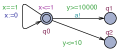
$\mathcal{A}_{2}$

$\mathcal{A}_{3}$

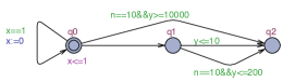
Figure 2: Examples explaining gains obtained with the algorithm.

The automaton $\mathcal{A}_{1}$ in Figure 2 illustrates the gain on the CSMA/CD protocol. The transition from $q_{0}$ to $q_{1}$ is disabled as it must synchronize on letter $a!$. The static analysis algorithm [2] ignores this fact, hence it associates bound $10^{4}$ to $y$ in $q_{0}$. Since our algorithm computes the bounds on-the-fly, $y$ is associated the bound $10$ in every node $(q_{0},Z)$. We observe that UPPAAL’s algorithm visits $10003$ nodes on $ZG(\mathcal{A}_{1})$ whereas our algorithm only visits $2$ nodes. The same situation occurs in the CSMA/CD example. However despite the improvement in the number of nodes (roughly $10\%$) the cost of computing the bounds impacts the running time negatively.

The gains that we observe in the analysis of the Fischer’s protocol are explained by the automaton $\mathcal{A}_{3}$ in Figure 2. $\mathcal{A}_{3}$ has a bounded integer variable $n$ that is initialized to $0$. Hence, the transitions from $q_{0}$ to $q_{2}$, and from $q_{1}$ to $q_{2}$, that check if $n$ is equal to $10$ are disabled. This is ignored by the static analysis algorithm that associates the bound $10^{4}$ to clock $y$ in $q_{0}$. Our algorithm however associates the bound $10$ to $y$ in every node $(q_{0},Z)$. We observe that UPPAAL’s algorithm visits $10004$ nodes whereas our algorithm only visits $3$ nodes. A similar situation occurs in the Fischer’s protocol. We include the last row to underline that our implementation is not as mature as UPPAAL. We strongly think that UPPAAL could benefit from methods presented here.

The second kind of improvement comes from the $\operatorname{\mathit{Closure}}_{\alpha}$ abstraction that particularly improves the analysis of the Fischer’s and the FDDI protocols. The situation observed on the FDDI protocol is explained in Figure 2. For the zone $Z$ in the figure, by definition $Extra_{LU}^{+}(Z)=Z$, and in consequence $Z^{\prime}\not\subseteq Z$. However, $Z^{\prime}\subseteq\operatorname{\mathit{Closure}}_{\alpha}(Z)$. On FDDI and Fischer’s protocols, our algorithm performs better due to the non-convex approximation.

6 Conclusions

We have proposed a new algorithm for checking reachability properties of timed automata. The algorithm has two sources of improvement that are quite independent: the use of the $\operatorname{\mathit{Closure}}_{\alpha}$ operator, and the computation of bound functions on-the-fly.

Apart from immediate gains presented in Table 1, we think that our approach opens some new perspectives on analysis of timed systems. We show that the use of non-convex approximations can be efficient. We have used very simple approximations, but it may be well the case that there are more sophisticated approximations to be discovered. The structure of our algorithm permits to calculate bounding constants on the fly. One should note that standard benchmarks are very well understood and very well modeled. In particular they have no “superfluous” constraints or clocks. However in not-so-clean models coming from systems in practice one can expect the on-the-fly approach to be even more beneficial.

There are numerous directions for further research. One of them is to find other approximation operators. Methods for constraint propagation also deserve a closer look. We believe that our approximations methods are compatible with partial order reductions [12, 14]. We hope that the two techniques can benefit from each other.

Appendix 0.A Proofs from Section 3

We provide all the proofs from the section presenting the efficient inclusion testing algorithm. For convenience, we recall the statements of the facts that are proven together with their original numbering. They are preceded with black arrow for readability.

$\blacktriangleright$Proposition 1.  A distance graph $G$ has only positive cycles iff ${[\![G]\!]}\not=\emptyset$.

Proof.

If there is a valuation $v\in{[\![G]\!]}$ then we replace every edge $x\stackrel{{\scriptstyle\preccurlyeq c}}{{\longrightarrow}}y$ by $x\stackrel{{\scriptstyle\leq d}}{{\longrightarrow}}y$ where $d=v(y)-v(x)$. We have $d\preccurlyeq_{xy}c_{xy}$. Since every cycle in the new graph has value $0$, every cycle in $G$ is positive.

For the other direction suppose that every cycle in $G$ is positive. Let $\overline{G}$ be the canonical form of $G$. Clearly ${[\![G]\!]}={[\![\overline{G}]\!]}$, i.e., the constraints defined by $G$ and by $\overline{G}$ are equivalent. It is also evident that all the cycles in $\overline{G}$ are positive.

We say that a variable $x$ is fixed in $\overline{G}$ if in this graph we have edges $0\stackrel{{\scriptstyle\leq c_{x}}}{{\longrightarrow}}x$ and $x\stackrel{{\scriptstyle\leq-c_{x}}}{{\longrightarrow}}0$ for some constant $c_{x}$. These edges mean that every valuation in ${[\![\overline{G}]\!]}$ should assign $c_{x}$ to $x$.

If all the variables in $\overline{G}$ are fixed then the value of every cycle in $\overline{G}$ is $0$, and the valuation assigning $c_{x}$ to $x$ for every variable $x$ is the unique valuation in ${[\![\overline{G}]\!]}$. Hence, ${[\![\overline{G}]\!]}$, and in consequence ${[\![G]\!]}$ are not empty.

Otherwise there is a variable, say $y$, that is not fixed in $\overline{G}$. We will show how to fix it. Let us multiply all the constraints in $\overline{G}$ by $2$. This means that we change each arrow $x_{1}\stackrel{{\scriptstyle\preccurlyeq c}}{{\longrightarrow}}x_{2}$ to $x_{1}\stackrel{{\scriptstyle\preccurlyeq 2c}}{{\longrightarrow}}x_{2}$. Let us call the resulting graph $H$. Clearly $H$ is in canonical form since $\overline{G}$ is. Moreover ${[\![H]\!]}$ is not empty iff ${[\![\overline{G}]\!]}$ is not empty. The gain of this transformation is that for our chosen variable $y$ we have in $H$ edges $0\stackrel{{\scriptstyle\preccurlyeq c_{0y}}}{{\longrightarrow}}y$ and $y\stackrel{{\scriptstyle\preccurlyeq c_{y0}}}{{\longrightarrow}}0$ with $c_{y0}+c_{0y}\geq 2$. This means that there is a natural number $d$ such that $(\leq,d)\leq(\preccurlyeq c_{0y})$ and $(\leq,-d)\leq(\preccurlyeq c_{y0})$. Let $H_{d}$ be $H$ with edges to and from $y$ changed to $0\stackrel{{\scriptstyle\leq d}}{{\longrightarrow}}y$ and $y\stackrel{{\scriptstyle\leq-d}}{{\longrightarrow}}0$, respectively. This is a distance graph where $y$ is fixed. We need to show that there is no negative cycle in this graph.

Suppose that there is a negative cycle in $H_{d}$. Clearly it has to pass through $0$ and $y$ since there was no negative cycle in $H$. Suppose that it uses the edge $0\stackrel{{\scriptstyle\leq d}}{{\longrightarrow}}y$, and suppose that the next used edge is $y\stackrel{{\scriptstyle\preccurlyeq c_{yx}}}{{\longrightarrow}}x$. The cycle cannot come back to $y$ before ending in $0$ since then we could construct a smaller negative cycle. Hence all the other edges in the cycle come from $H$. Since $H$ is in the canonical form, a path from $x$ to $0$ can be replaced by the edge from $x$ to $0$, and the value of the path will not increase. This means that our hypothetical negative cycle has the form $0\stackrel{{\scriptstyle\leq d}}{{\longrightarrow}}y\stackrel{{\scriptstyle\preccurlyeq c_{yx}}}{{\longrightarrow}}x\stackrel{{\scriptstyle\preccurlyeq c_{x0}}}{{\longrightarrow}}0$. By canonicity of $H$ we have $(\preccurlyeq_{yx},c_{yx})+(\preccurlyeq_{x0},c_{x0})\geq(\preccurlyeq_{y0},c_{y0})$. Putting these two facts together we get

$$(\leq,0)>(\leq,d)+(\preccurlyeq_{yx},c_{yx})+(\preccurlyeq_{x0},c_{x0})\geq(\leq,d)+(\preccurlyeq_{y0},c_{y0})$$

but this contradicts the choice of $d$ which supposed that $(\leq,d)+(\preccurlyeq_{y0},c_{y0})$ is positive. The proof when the hypothetical negative cycle passes through the edge $y\stackrel{{\scriptstyle\leq-d}}{{\longrightarrow}}0$ is analogous.

Summarizing, starting from $G$ that has no negative cycles we have constructed a graph $H_{d}$ that has no negative cycles, and has one more variable fixed. We also know that if ${[\![H_{d}]\!]}$ is not empty then ${[\![G]\!]}$ is not empty. Repeatedly applying this construction we get a graph where all the variables are fixed and no cycle is negative. As we have seen above the semantics of such a graph is not empty. ∎∎

$\blacktriangleright$Proposition 2.  Let $R$ be a region and let $Z$ be a zone. The intersection $R\cap Z$ is empty iff there exist variables $x,y$ such that $Z_{yx}+R_{xy}\leq(<,0)$.

Before proving the above proposition, we will start with some notions. Let $R$ be a region wrt. a bound function $\alpha:X\to\mathbb{N}$. A variable $x$ is bounded in $R$ if a constraint $x\leq c$ holds in $R$ for some constant $c$; otherwise the variable is called unbounded in $R$. Observe that if $x_{1},x_{2}$ are bounded then we have

$$x_{1}-x_{2}=c c-1<x_{1}-x_{2}<c R$$ or  in .

If $y$ is unbounded then we have $y>\alpha_{y}$ in $R$.

For two distance graphs $G_{1}$, $G_{2}$ which are not necessarily in canonical form, we denote by $\min(G_{1},G_{2})$ the distance graph where each edge has the weight equal to the minimum of the corresponding weights in $G_{1}$ and $G_{2}$. Even though this graph may be not in canonical form, it should be clear that it represents intersection of the two arguments, that is, ${[\![\min(G_{1},G_{2})]\!]}={[\![G_{1}]\!]}\cap{[\![G_{2}]\!]}$; in other words, the valuations satisfying the constraints given by $\min(G_{1},G_{2})$ are exactly those satisfying all the constraints from $G_{1}$ as well as $G_{2}$.

We are now ready to examine the conditions when $R\cap Z$ is empty. We start with the following simple lemma.

Lemma 2

Let $G_{R}$ be the distance graph of a region and let $x_{1},x_{2}$ be two variables bounded in $R$. For every distance graph $G$: if in $\min(G_{R},G)$ the weight of the edge $x_{1}\stackrel{{\scriptstyle}}{{\longrightarrow}}x_{2}$ comes from $G$ then $x_{1}\stackrel{{\scriptstyle}}{{\longrightarrow}}x_{2}\stackrel{{\scriptstyle}}{{\longrightarrow}}x_{1}$ is a negative cycle in $\min(G_{R},G)$.

Proof.

Suppose that the edge $x_{1}\stackrel{{\scriptstyle\preccurlyeq c}}{{\longrightarrow}}x_{2}$ is as required by the assumption of the lemma. In $R$ we can have either $x_{2}-x_{1}=d$ or $d-1<x_{2}-x_{1}<d$.

In the first case we have edges $x_{1}\stackrel{{\scriptstyle\leq d}}{{\longrightarrow}}x_{2}$ and $x_{2}\stackrel{{\scriptstyle\leq-d}}{{\longrightarrow}}x_{1}$ in $G_{R}$. Since the edge $x_{1}\stackrel{{\scriptstyle\preccurlyeq c}}{{\longrightarrow}}x_{2}$ comes from $G$ we have $c<d$ or $c=d$ and $\preccurlyeq$ is the strict inequality. We get a negative cycle $x_{1}\stackrel{{\scriptstyle\preccurlyeq c}}{{\longrightarrow}}x_{2}\stackrel{{\scriptstyle\leq-d}}{{\longrightarrow}}x_{1}$.

In the second case we have edges $x_{2}\stackrel{{\scriptstyle<-d+1}}{{\longrightarrow}}x_{1}$ and $x_{1}\stackrel{{\scriptstyle<d}}{{\longrightarrow}}x_{2}$ in $R$. Hence $c<d$ and $x_{1}\stackrel{{\scriptstyle\preccurlyeq c}}{{\longrightarrow}}x_{2}\stackrel{{\scriptstyle<-d+1}}{{\longrightarrow}}x_{1}$ gives a negative cycle. ∎∎

Proof of Proposition 2

Let $G_{R}$, $G_{Z}$ be the canonical distance graphs representing the region $R$ and the zone $Z$ respectively. One direction is immediate: If $\min(G_{R},G_{Z})$ has a negative cycle then $R\cap Z$ is empty by Proposition 1.

For the other direction suppose that $R\cap Z$ is empty. Again, by Proposition 1 the graph $\min(G_{R},G_{Z})$ has a negative cycle. An immediate case is when in this graph an edge between two variables bound in $R$ comes from $G_{Z}$. From Lemma 2 we obtain a negative cycle on these two variables. So in what follows we suppose that in $\min(G_{R},G_{Z})$ all the edges between variables bounded in $R$ come from $G_{R}$. Hence every negative cycle should contain an unbounded variable.

Let $y$ be a variable unbounded in $R$ that is a part of the negative cycle. Consider $y$ with its successor and its predecessor on the cycle: $x\stackrel{{\scriptstyle}}{{\longrightarrow}}y\stackrel{{\scriptstyle}}{{\longrightarrow}}x^{\prime}$. We will show that we can assume that $x^{\prime}$ is $x_{0}$. Observe that in $G_{R}$ every edge to $y$ has value $\infty$. So the weight of the edge $x\stackrel{{\scriptstyle}}{{\longrightarrow}}y$ is from $G_{Z}$. If the weight of the outgoing edge is also from $G_{Z}$ then we could have eliminated $y$ from the cycle by choosing $x\stackrel{{\scriptstyle}}{{\longrightarrow}}x^{\prime}$ from $G_{Z}$. Hence the weight of $y\stackrel{{\scriptstyle}}{{\longrightarrow}}x^{\prime}$ comes from $G_{R}$. Since $y$ is unbounded in $R$, the weight of this edge is $d-\alpha_{y}$, where $d$ is the value on the edge $0\stackrel{{\scriptstyle\preccurlyeq d}}{{\longrightarrow}}x^{\prime}$ in $G_{R}$. This is because we can rewrite inequation $x^{\prime}-y<d-\alpha_{y}$ as $y-x^{\prime}>\alpha_{y}-d$, and we know that $\alpha_{y}$ is the smallest possible value for $y$, while $d$ is the supremum on the possible values of $x^{\prime}$. But then instead of the edge $y\stackrel{{\scriptstyle}}{{\longrightarrow}}x^{\prime}$ we can take $y\stackrel{{\scriptstyle}}{{\longrightarrow}}x_{0}\stackrel{{\scriptstyle}}{{\longrightarrow}}x^{\prime}$ in $\min(G_{R},G_{Z})$ which has smaller value since we have $y\stackrel{{\scriptstyle<-\alpha_{y}}}{{\longrightarrow}}x_{0}$ in $G_{R}$.

If $x$ is $x_{0}$ then we get a cycle of a required form since it contains only $x_{0}$ and $y$. Otherwise, let us more closely examine the whole negative cycle:

$$x_{0}\stackrel{{\scriptstyle}}{{\longrightarrow}}x_{i_{1}}\stackrel{{\scriptstyle}}{{\longrightarrow}}\dots\stackrel{{\scriptstyle}}{{\longrightarrow}}x_{i_{k}}\stackrel{{\scriptstyle}}{{\longrightarrow}}x\stackrel{{\scriptstyle}}{{\longrightarrow}}y\stackrel{{\scriptstyle}}{{\longrightarrow}}x_{0}\ .$$

By the reasoning from the previous paragraph, all of $x_{i_{1}},\dots,x_{i_{k}}$ can be assumed to be bounded in $R$. Otherwise we could get a cycle visiting $x_{0}$ twice and we could remove a part of it with one unbounded variable and still have a negative cycle. By our assumption, all the edges from and to these variables come from $R$. This means that the path from $x_{0}$ to $x$ can be replaced by an edge $x_{0}\stackrel{{\scriptstyle}}{{\longrightarrow}}x$ from $R$. So finally, the negative cycle has the required form $x_{0}\stackrel{{\scriptstyle}}{{\longrightarrow}}x\stackrel{{\scriptstyle}}{{\longrightarrow}}y\stackrel{{\scriptstyle}}{{\longrightarrow}}x_{0}$ with the edges $x_{0}\xrightarrow{}x$ and $y\xrightarrow{}x_{0}$ coming from $G_{R}$ and the edge $x\xrightarrow{}y$ coming from $G_{Z}$. Since $G_{R}$ is canonical, we can reduce this cycle to $x\xrightarrow{}y\xrightarrow{}x$ with $x\xrightarrow{}y$ coming from $G_{Z}$ and $y\xrightarrow{}x$ coming from $G_{R}$.∎

0.A.1 Efficient inclusion testing

Given two zones $Z$ and $Z^{\prime}$ and a bound function $\alpha$, we would like to know if $Z\not\subseteq\operatorname{\mathit{Closure}}_{\alpha}(Z^{\prime})$: that is, does there exist a region $R$ that intersects $Z$ but does not intersect $Z^{\prime}$? From Proposition 2 this reduces to asking if there exists a region $R$ that intersects $Z$ and two variables $x,y$ such that $Z^{\prime}_{yx}+R_{xy}<(\leq,0)$. This brings us to look for the least value of $R_{xy}$ from among the regions $R$ intersecting $Z$. We begin with the observation that every consistent instantiation of an edge in a canonical distance graph $G$ gives a valuation satisfying the constraints of $G$.

$\blacktriangleright$Lemma 1.  Let $G$ be a distance graph in canonical form, with all cycles positive. Let $x,y$ be two variables such that $x\stackrel{{\scriptstyle\preccurlyeq_{xy}c_{xy}}}{{\longrightarrow}}y$ and $y\stackrel{{\scriptstyle\preccurlyeq_{yx}c_{yx}}}{{\longrightarrow}}x$ are edges in $G$. Let $d\in\mathbb{R}$ such that $d\preccurlyeq_{xy}c_{xy}$ and $-d\preccurlyeq_{yx}c_{yx}$. Then, there exists a valuation $v\in{[\![G]\!]}$ such that $v(y)-v(x)=d$.

Proof.

Take $d$ as in the assumption of the lemma. Let $G_{d}$ be the distance graph where we have the edges $x\stackrel{{\scriptstyle\leq d}}{{\longrightarrow}}y$, and $y\stackrel{{\scriptstyle\leq-d}}{{\longrightarrow}}x$ for variables $x$ and $y$ and the rest of the edges come from $G$. We show that all cycles in $G_{d}$ are positive. For contradiction, suppose there is a negative cycle $N$ in $G_{d}$. Clearly, since $G$ does not have negative cycle, $N$ should contain the variables $x$ and $y$. The value of the shortest path from $x$ to $y$ in $G$ was given by $(\preccurlyeq_{xy},c_{xy})$. Therefore, the shortest path value from $x$ to $y$ in $G_{d}$ is given by $d$ and the shortest path value from $y$ to $x$ is $-d$. Hence the sum of the weights in $N$ is negative would imply that the value of the cycle $x\rightarrow y\rightarrow x$ is negative. However since, this is $0$, such a negative cycle $N$ cannot exist. The lemma follows from Proposition 1. ∎∎

Recall that for a zone $Z$, we denote by $Z_{xy}$ the weight of the edge $x\xrightarrow{\preccurlyeq_{xy}c_{xy}}y$ in the canonical distance graph representing $Z$. We denote by $[v]$ the region to which $v$ belongs to; $[v]_{xy}$ denotes the value $(\preccurlyeq_{xy},r_{xy})$ of the constraint $y-x\preccurlyeq_{xy}r_{xy}$ defining the region $[v]$. This is precisely the value of the edge $x\xrightarrow{\preccurlyeq_{xy}r_{xy}}y$ in the canonical distance graph representing the region $[v]$. We are interested in finding the least value of $[v]_{xy}$ from among the valuations $v\in Z$. Lemmas 3 and 4 describe this least value of $[v]_{xy}$ for different combinations of $x$ and $y$.

For a weight $(\preccurlyeq,c)$ we define $-(\preccurlyeq,c)$ as $(\preccurlyeq,-c)$. We now define a ceiling function $\lceil\cdot\rceil$ for weights.

Definition 1

For a real $c$, let $\lceil c\rceil$ denote the smallest integer that is greater than or equal to $c$. We define the ceiling function $\lceil(\preccurlyeq,c)\rceil$ for a weight $(\preccurlyeq,c)$ depending on whether $\preccurlyeq$ equals $\leq$ or $<$, as follows:

$$\lceil(\leq,c)\rceil=\begin{cases}(\leq,c)&\text{if }c\text{ is an integer}\\ (<,\lceil c\rceil)&\text{otherwise }\end{cases}$$

$$\lceil(<,c)\rceil=\begin{cases}(<,c+1)&\text{if }c\text{ is an integer}\\ (<,\lceil c\rceil)&\text{otherwise }\end{cases}$$

Lemma 3

Let $Z$ be a non-empty zone and let $x$ be a variable different from $x_{0}$. Then, from among the regions $R$ that intersect $Z$:

• the least value of $R_{0x}$ is given by

  $$\begin{cases}(<,\infty)&\text{if }Z_{x0}<(\leq,-\alpha_{x})\\ \lceil-Z_{x0}\rceil&\text{otherwise}\end{cases}$$

• the least value of $R_{x0}$ is given by $\max\{\lceil-Z_{0x}\rceil,(<,-\alpha_{x})\}$.

Proof.

Let $Z_{0x}=(\preccurlyeq_{0x},c_{0x})$ and $Z_{x0}=(\preccurlyeq_{x0},c_{x0})$.

For the least value of $R_{0x}$, first note that if $Z_{x0}<(\leq,-\alpha_{x})$ then all valuations $v\in Z$ have $v_{x}>\alpha_{x}$ and by definition $[v]_{0x}=(<,\infty)$ for such valuations. If not, we know that for all valuations $-v_{x}\preccurlyeq_{x0}c_{x0}$, that is, $v_{x}\succcurlyeq_{x0}-c_{x0}$. If $\preccurlyeq_{x0}$ is $\leq$, then from Lemma 1 there exists a valuation with $v_{x}=-c_{x0}$ and this is the minimum value that can be attained. When $\preccurlyeq_{x0}$ is $<$, then we can find a positive $\epsilon<1$ such that $c_{x0}-\epsilon\preccurlyeq_{x0}c_{x0}$ and $-c_{x0}+\epsilon\preccurlyeq_{0x}c_{0x}$. From Lemma 1, there exists a valuation with $v_{x}=-c_{x0}+\epsilon$ for which $[v]_{0x}=(<,-c_{x0}+1)$. Since $\preccurlyeq_{x0}$ is a strict $<$, this is the minimum value for $R_{0x}$. This gives that the minimum value is $\lceil-Z_{x0}\rceil$.

Now we look at the minimum value for $R_{x0}$. If $(\preccurlyeq_{0x},c_{0x})\leq(\leq,\alpha_{x})$, then all valuations $v$ have $v_{x}\leq\alpha_{x}$ and by an argument similar to above, the minimum value of $R_{x0}$ would be given by $\lceil-Z_{0x}\rceil$. Since $(\preccurlyeq_{0x},c_{0x})\leq(\leq,\alpha_{x})$, we have $(\preccurlyeq_{0x},-c_{0x})\geq(\leq,-\alpha_{x})>(<,-\alpha_{x})$. If $(\preccurlyeq_{0x},c_{0x})>(\leq,\alpha_{x})$, then from Lemma 1, there are valuations in $Z$ with $v_{x}>\alpha_{x}$ and for these valuations, $[v]_{x0}=(<,-\alpha_{x})$. In this case the minimum value is given by $(<,-\alpha_{x})$. Since $(\preccurlyeq_{0x},c_{0x})>(\leq,\alpha_{x})$, we have $(\preccurlyeq_{0x},-c_{0x})<(<,-\alpha_{x})$ and so $\lceil-Z_{0x}\rceil\leq(<,-\alpha_{x})$. In each case, observe that we get $\max\{\lceil-Z_{0x}\rceil,(<,-\alpha_{x})\}$ as the minimum value. ∎∎

Lemma 4

Let $Z$ be a non-empty zone and let $x,y$ be variables none of them equal to $x_{0}$. Then, from among the regions $R$ that intersect $Z$, the least value of $R_{xy}$ is given by

$$\begin{cases}(<,\infty)&\text{ if }Z_{y0}<(\leq,-\alpha_{y})\\ \max\{\lceil-Z_{yx}\rceil,\lceil-Z_{y0}\rceil-(\leq,\alpha_{x})\}&\text{ otherwise}\end{cases}$$

Proof.

Let $G$ be the canonical distance graph representing the zone $Z$. We denote the weight of an edge $i\xrightarrow{}j$ in $G$ by $(\preccurlyeq_{ij},c_{ij})$. Recall that this means $Z_{ij}=(\preccurlyeq_{ij},c_{ij})$. For clarity, for a valuation $v$, we write $v_{x}$ for $v(x)$.

We are interested in computing the smallest value of the $y-x$ constraint defining a region belonging to $\operatorname{\mathit{Closure}}_{\alpha}(Z)$, that is, we need to find $\min\{[v]_{xy}~{}|~{}v\in Z\}$. Call this $\beta$. By definition of regions, we have for a valuation $v$:

$$[v]_{xy}=\begin{cases}(<,\infty)&\text{if }v_{y}>\alpha_{y}\\ \lceil(\leq,v_{y}-v_{x})\rceil&\text{if }v_{y}\leq\alpha_{y}\text{ and }v_{x}\leq\alpha_{x}\\ (<,\lceil v_{y}\rceil-\alpha_{x})&\text{if }v_{y}\leq\alpha_{y}\text{ and }v_{x}>\alpha_{x}\end{cases}$$ (2)

We now consider the first of the two cases from the statement of the lemma. Namely, $Z_{y0}<(\leq,-\alpha_{y})$. This means that $0-v_{y}\preccurlyeq_{y0}c_{y0}$ and $c_{y0}\leq-\alpha_{y}$; moreover $\preccurlyeq_{y0}$ is the strict inequality if $c_{y0}=-\alpha_{y}$. In consequence, all valuations $v\in Z$, satisfy $v_{y}>\alpha_{y}$. Whence $\beta=(<,\infty)$.

We now consider the case when $Z_{y0}\geq(\leq,-\alpha_{y})$. Let $G^{\prime}$ be the graph in which the edge $0\xrightarrow{}y$ has weight $\min\{(\leq,\alpha_{y}),(\preccurlyeq_{0y},c_{0y})\}$ and the rest of the edges are the same as that of $G$. This graph $G^{\prime}$ represents the valuations of $Z$ that have $v_{y}\leq\alpha_{y}$: ${[\![G^{\prime}]\!]}=\{v\in Z~{}|~{}v_{y}\leq\alpha_{y}\}$. We show that this set is not empty. For this we check that $G^{\prime}$ does not have negative cycles. Since $G$ does not have negative cycles, every negative cycle in $G^{\prime}$ should include the newly modified edge $0\xrightarrow{}y$. Note that the shortest path value from $y$ to $0$ does not change due to this modified edge. So the only possible negative cycle in $G^{\prime}$ is $0\xrightarrow{}y\xrightarrow{}0$. But then we are considering the case when $Z_{y0}\geq(\leq,-\alpha_{y})$, and so $Z_{y0}+(\leq,\alpha_{y})\geq(\leq,0)$. Hence this cycle cannot be negative either. In consequence all the cycles in $G^{\prime}$ are positive and ${[\![G^{\prime}]\!]}$ is not empty.

To find $\beta$, it is sufficient to consider only the valuations in ${[\![G^{\prime}]\!]}$. As seen from Equation 2, among the valuations in ${[\![G^{\prime}]\!]}$, we need to differentiate between those with $v_{x}\leq\alpha_{x}$ and the ones with $v_{x}>\alpha_{x}$. We proceed as follows. We first compute $\min\{[v]_{xy}~{}|~{}v\in{[\![G^{\prime}]\!]}\text{ and }v_{x}\leq\alpha_{x}\}$. Call this $\beta_{1}$. Next, we compute $\min\{[v]_{xy}~{}|~{}v\in{[\![G^{\prime}]\!]}\text{ and }v_{x}>\alpha_{x}\}$ and set this as $\beta_{2}$. Our required value $\beta$ would then equal $\min\{\beta_{1},\beta_{2}\}$.

To compute $\beta_{1}$, consider the following distance graph $G^{\prime}_{1}$ which is obtained from $G^{\prime}$ by just changing the edge $0\xrightarrow{}x$ to $\min\{(\leq,\alpha_{x}),(\preccurlyeq_{0x},c_{0x})\}$ and keeping the remaining edges the same as in $G^{\prime}$. The set of valuations ${[\![G^{\prime}_{1}]\!]}$ equals $\{v\in{[\![G^{\prime}]\!]}~{}|~{}v_{x}\leq\alpha_{x}\}$. If ${[\![G^{\prime}_{1}]\!]}=\emptyset$, we set $\beta_{1}$ to $(<,\infty)$ and proceed to calculate $\beta_{2}$. If not, we see that from Equation 2, for every $v\in{[\![G^{\prime}_{1}]\!]}$, $[v]_{xy}$ is given by $\lceil(\leq,v_{y}-v_{x})\rceil$. Let $(\preccurlyeq_{1},w_{1})$ be the shortest path from $y$ to $x$ in the graph $G^{\prime}_{1}$. Then, we have for all $v\in{[\![G^{\prime}_{1}]\!]}$, $v_{x}-v_{y}\preccurlyeq_{1}w_{1}$, that is, $v_{y}-v_{x}\succcurlyeq_{1}-w_{1}$. If $\preccurlyeq_{1}$ is $\leq$, then the least value of $[v]_{xy}$ would be $(\leq,-w_{1})$ and if $\preccurlyeq_{1}$ is $<$, one can see that the least value of $[v]_{xy}$ is $(<,-w_{1}+1)$. This shows that $\beta_{1}=\lceil(\preccurlyeq_{1},-w_{1})\rceil$. It now remains to calculate $(\preccurlyeq_{1},w_{1})$.

Recall that $G^{\prime}_{1}$ has the same edges as in $G$ except possibly different edges $0\xrightarrow{}x$ and $0\xrightarrow{}y$. If the shortest path from $y$ to $x$ has changed in $G^{\prime}_{1}$, then clearly it should be due to one of the above two edges. However note that the edge $0\xrightarrow{}y$ cannot belong to the shortest path from $y$ to $x$ since it would contain a cycle $y\xrightarrow{}\dots 0\xrightarrow{}y\xrightarrow{}\dots x$ that can be removed to give shorter path. Therefore, only the edge $0\xrightarrow{}x$ can potentially yield a shorter path: $y\xrightarrow{}\dots\xrightarrow{}0\xrightarrow{}x$. However, the shortest path from $y$ to $0$ in $G^{\prime}_{1}$ cannot change due to the added edges since that would form a cycle with $0$ and we know that all cycles in $G^{\prime}_{1}$ are positive. Therefore the shortest path from $y$ to $0$ is the direct edge $y\xrightarrow{}0$, and the shortest path from $y$ to $x$ is the minimum of the direct edge $y\xrightarrow{}x$ and the path $y\xrightarrow{}0\xrightarrow{}x$. We get: $(\preccurlyeq_{1},w_{1})=\min\{(\preccurlyeq_{yx},c_{yx}),(\preccurlyeq_{y0},c_{y0})+(\leq,\alpha_{x})\}$ which equals $\min\{Z_{yx},Z_{y0}+(\leq,\alpha_{x})\}$. Finally, from the argument in the above two paragraphs, we get:

$$\beta_{1}=\begin{cases}(<,\infty)&\text{ if }{[\![G^{\prime}_{1}]\!]}=\emptyset\\ \lceil-Z_{yx}\rceil&\text{ if }{[\![G^{\prime}_{1}]\!]}\neq\emptyset\text{ and }Z_{yx}\leq Z_{y0}+(\leq,\alpha_{x})\\ \lceil-Z_{y0}\rceil+(\leq,-\alpha_{x})&\text{ if }{[\![G^{\prime}_{1}]\!]}\neq\emptyset\text{ and }Z_{yx}>Z_{y0}+(\leq,\alpha_{x})\\ \end{cases}$$ (3)

We now proceed to compute $\beta_{2}=\min\{[v]_{xy}~{}|~{}v\in{[\![G^{\prime}]\!]}\text{ and }v_{x}>\alpha_{x}\}$. Let $G^{\prime}_{2}$ be the graph which is obtained from $G^{\prime}$ by modifying the edge $x\xrightarrow{}0$ to $\min\{Z_{x0},(<,-\alpha_{x})\}$ and keeping the rest of the edges the same as in $G^{\prime}$. Clearly ${[\![G^{\prime}_{2}]\!]}=\min\{v\in{[\![G^{\prime}]\!]}~{}|~{}v_{x}>\alpha_{x}\}$.

Again, if ${[\![G^{\prime}_{2}]\!]}$ is empty, we set $\beta_{2}$ to $(<,\infty)$. Otherwise, from Equation 2, for each valuation $v\in{[\![G^{\prime}_{2}]\!]}$, the value of $[v]_{xy}$ is given by $(<,\lceil v_{y}\rceil-\alpha_{x})$. For the minimum value, we need the least value of $v_{y}$ from $v\in{[\![G^{\prime}_{2}]\!]}$. Let $(\preccurlyeq_{2},w_{2})$ be the shortest path from $y$ to $0$ in $G^{\prime}_{2}$. Then, since $-v_{y}\preccurlyeq_{2}w_{2}$, the least value of $\lceil v_{y}\rceil$ would be $-w_{2}$ if $\preccurlyeq_{2}=\leq$ and equal to $\lceil-w_{2}\rceil$ if $\preccurlyeq_{2}=<$ and $\beta_{2}$ would respectively be $(<,-w_{2}-\alpha_{x})$ or $(<,-w_{2}+1-\alpha_{x})$. It now remains to calculate $(\preccurlyeq_{2},w_{2})$.

Recall that $G^{\prime}_{2}$ is $G$ with $0\xrightarrow{}y$ and $x\xrightarrow{}0$ modified. The shortest path from $y$ to $0$ cannot include the edge $0\xrightarrow{}y$ since it would need to contain a cycle, for the same reasons as in the $\beta_{1}$ case. So we get $(\preccurlyeq_{2},w_{2})=\min\{Z_{y0},Z_{yx}+(<,-\alpha_{x})\}$. If $Z_{y0}\leq Z_{yx}+(<,-\alpha_{x})$, then we take $(\preccurlyeq_{2},w_{2})$ as $Z_{y0}$, otherwise we take it to be $Z_{yx}+(<,-\alpha_{x})$. So, we get $\beta_{2}$ as the following:

$$\beta_{2}=\begin{cases}(<,\infty)&\text{ if }{[\![G^{\prime}_{2}]\!]}=\emptyset\\ -Z_{yx}+(<,1)&\text{ if }{[\![G^{\prime}_{2}]\!]}\neq\emptyset\text{ and }Z_{y0}\geq Z_{yx}+(<,-\alpha_{x})\\ \lceil-Z_{y0}\rceil+(<,-\alpha_{x})&\text{ if }{[\![G^{\prime}_{2}]\!]}\neq\emptyset\text{ and }Z_{y0}<Z_{yx}+(<,-\alpha_{x})\\ \end{cases}$$ (4)

However, we would like to write $\beta_{2}$ in terms of the cases used for $\beta_{1}$ in Equation 3 so that we can write $\beta$, which equals $\min\{\beta_{1},\beta_{2}\}$, conveniently.

Let $\psi_{1}$ be the inequation: $Z_{yx}\leq Z_{y0}+(\leq,\alpha_{x})$. From Equation 3, note that $\beta_{1}$ has been classified according to $\psi_{1}$ and $\neg\psi_{1}$ when ${[\![G^{\prime}_{1}]\!]}$ is not empty. Similarly, let $\psi_{2}$ be the inequation: $Z_{y0}\geq Z_{yx}+(<,-\alpha_{x})$. From Equation 4 we see that $\beta_{2}$ has been classified in terms of $\psi_{2}$ and $\neg\psi_{2}$ when ${[\![G^{\prime}_{2}]\!]}$ is not empty. Notice the subtle difference between $\psi_{1}$ and $\psi_{2}$ in the weight component involving $\alpha_{x}$: in the former the inequality associated with $\alpha_{x}$ is $\leq$ and in the latter it is $<$. This necessitates a bit more of analysis before we can write $\beta_{2}$ in terms of $\psi_{1}$ and $\neg\psi_{1}$.

Suppose $\psi_{1}$ is true. So we have $(\preccurlyeq_{yx},c_{yx})\leq(\preccurlyeq_{y0},c_{y0}+\alpha_{x})$. This implies: $c_{yx}\leq c_{y0}+\alpha_{x}$. Therefore, $c_{y0}\geq c_{yx}-\alpha_{x}$. When $c_{y0}>c_{yx}-\alpha_{x}$, $\psi_{2}$ is clearly true. For the case when $c_{y0}=c_{yx}-\alpha_{x}$, note that in $\psi_{2}$ the right hand side is always of the form $(<,c_{yx}-\alpha_{x})$, irrespective of the inequality in $Z_{yx}$ and so yet again, $\psi_{2}$ is true. We have thus shown that $\psi_{1}$ implies $\psi_{2}$.

Suppose $\neg\psi_{1}$ is true. We have $(\preccurlyeq_{yx},c_{yx})>(\preccurlyeq_{y0},c_{y0}+\alpha_{x})$. If $c_{yx}>c_{y0}+\alpha_{x}$, then clearly $c_{y0}<c_{yx}-\alpha_{x}$ implying that $\neg\psi_{2}$ holds. If $c_{yx}=c_{y0}+\alpha_{x}$, then we need to have $\preccurlyeq_{yx}=\leq$ and $\preccurlyeq_{y0}=<$. Although $\neg\psi_{2}$ does not hold now, we can safely take $\beta_{2}$ to be $\lceil-Z_{y0}\rceil+(<,-\alpha_{x})$ as its value is in fact equal to $-Z_{yx}+(<,1)$ in this case. Summarizing the above two paragraphs, we can rewrite $\beta_{2}$ as follows:

$$\beta_{2}=\begin{cases}(<,\infty)&\text{ if }{[\![G^{\prime}_{2}]\!]}=\emptyset\\ -Z_{yx}+(<,1)&\text{ if }{[\![G^{\prime}_{2}]\!]}\neq\emptyset\text{ and }Z_{xy}\leq Z_{y0}+(\leq,\alpha_{x})\\ \lceil-Z_{y0}\rceil+(<,-\alpha_{x})&\text{ if }{[\![G^{\prime}_{2}]\!]}\neq\emptyset\text{ and }Z_{xy}>Z_{y0}+(\leq,\alpha_{x})\\ \end{cases}$$ (5)

We are now in a position to determine $\beta$ as $\min\{\beta_{1},\beta_{2}\}$. Recall that we are in the case where $Z_{y0}\leq(\leq,-\alpha_{y})$ and we have established that ${[\![G^{\prime}]\!]}$ is non-empty. Now since ${[\![G^{\prime}]\!]}={[\![G^{\prime}_{1}]\!]}\cup{[\![G^{\prime}_{2}]\!]}$ by construction, both of them cannot be simultaneously empty. Hence from Equations 3 and 5, we get $\beta$, the $\min\{\beta_{1},\beta_{2}\}$ as:

$$\beta_{=}\begin{cases}\lceil-Z_{yx}\rceil&\text{ if }Z_{xy}\leq Z_{y0}+(\leq,\alpha_{x})\\ \lceil-Z_{y0}\rceil+(<,-\alpha_{x})&\text{ if }Z_{xy}>Z_{y0}+(\leq,\alpha_{x})\\ \end{cases}$$ (6)

There remains one last reasoning. To prove the lemma, we need to show that $\beta=\max\{\lceil-Z_{yx}\rceil,\lceil-Z_{y0}\rceil+(<,-\alpha_{x})\}$. For this it is enough to show the following two implications:

$$Z_{yx}\leq Z_{y0}+(\leq,\alpha_{x})\Rightarrow\lceil-Z_{yx}\rceil\geq\lceil-Z_{y0}\rceil+(<,-\alpha_{x})$$

$$Z_{yx}>Z_{y0}+(\leq,\alpha_{x})\Rightarrow\lceil-Z_{yx}\rceil\leq\lceil-Z_{y0}\rceil+(<,-\alpha_{x})$$

We prove only the first implication. The second follows in a similar fashion. Let us consider the notation $(\preccurlyeq_{yx},c_{yx})$ and $(\preccurlyeq_{y0},c_{y0})$ for $Z_{yx}$ and $Z_{y0}$ respectively. So we have:

$$(\preccurlyeq_{yx},c_{yx})\leq(\preccurlyeq_{y0},c_{y0})+(\leq,\alpha_{x})$$

$$\Rightarrow~{} (\preccurlyeq_{yx},c_{yx})\leq(\preccurlyeq_{y0},c_{y0}+\alpha_{x})$$

If the constant $c_{yx}<c_{y0}+\alpha_{x}$, then $-c_{yx}>-c_{y0}-\alpha_{x}$ and we clearly get that $\lceil-Z_{yx}\rceil\geq\lceil-Z_{y0}\rceil+(<,-\alpha_{x})$. If the constant $c_{yx}=c_{y0}+\alpha_{x}$ and if $\preccurlyeq_{y0}=\leq$, then the required inequation is trivially true; if $\preccurlyeq_{y0}=<$, it implies that $\preccurlyeq_{yx}=<$ too and clearly $\lceil(<,-c_{yx})\rceil$ equals $\lceil(<,-c_{y0})\rceil+(<,-\alpha_{x})$. ∎

∎

$\blacktriangleright$Theorem 3.1. Let $Z,Z^{\prime}$ be zones. Then, $Z\nsubseteq\operatorname{\mathit{Closure}}_{\alpha}(Z^{\prime})$ iff there exist variables $x$, $y$ such that one of the following conditions hold:

1. $Z^{\prime}_{0x}<Z_{0x}\text{ and }Z^{\prime}_{0x}\leq(\alpha_{x},\leq)$, or

2. $Z^{\prime}_{x0}<Z_{x0}\text{ and }Z_{x0}\geq(-\alpha_{x},\leq)$, or

3. $Z_{x0}\geq(-\alpha_{x},\leq)\text{ and }Z^{\prime}_{xy}<Z_{xy}\text{ and }Z^{\prime}_{xy}\leq(\alpha_{y},\leq)+\lfloor Z_{x0}\rfloor$

Proof.

By definition of the $\operatorname{\mathit{Closure}}$ abstraction, $Z\nsubseteq\operatorname{\mathit{Closure}}_{\alpha}(Z^{\prime})$ iff there exists a region $R$ that intersects $Z$ but does not intersect $Z^{\prime}$. Therefore, from Proposition 2, we need an $R$ that intersects $Z$ and satisfies $Z^{\prime}_{yx}+R_{xy}<(\leq,0)$ for some variables $x,y$. This is equivalent to saying that for the least value of $R_{xy}$ that can be obtained from the zone $Z$, we have $Z^{\prime}_{yx}+R_{xy}<(0,\leq)$. Depending on if $x$ is $x_{0}$ or $y$ is $x_{0}$ or both $x$ and $y$ are not $x_{0}$ we get the following three conditions that correspond to the three conditions given in the theorem.

Case 1: $Z^{\prime}_{0x}+R_{x0}<(\leq,0)$
From Lemma 3, the minimum value of $R_{x0}$ from among the regions intersecting $Z$ is given by $\max\{\lceil-Z_{0x}\rceil,(<,-\alpha_{x})\}$. So we have:

$$Z^{\prime}_{0x} +\max\{\lceil-Z_{0x}\rceil,(<,-\alpha_{x})\}<(\leq,0)$$

$$\Rightarrow~{}Z^{\prime}_{0x}+\lceil-Z_{0x}\rceil<(\leq,0)~{}\text{ and }~{}Z^{\prime}_{0x}+(<,-\alpha_{x})<(\leq,0)$$

$$\Rightarrow~{}Z^{\prime}_{0x}<Z_{0x}~{}\text{ and }~{}Z^{\prime}_{0x}\leq(\leq,\alpha_{x})$$

This gives Condition 1 of the theorem.

Case 2: $Z^{\prime}_{x0}+R_{0x}<(\leq,0)$
From Lemma 3, the minimum value of $R_{0x}$ is $(<,\infty)$ if $-Z_{x0}>(\leq,\alpha_{x})$ and hence it cannot be part of a negative cycle. The edge $R_{0x}$ can yield a negative cycle only when $-Z_{x0}\leq(\leq,\alpha_{x})$, in which case the least value of $R_{0x}$ is given by $\lceil-Z_{x0}\rceil$. So we have $Z^{\prime}_{x0}+\lceil-Z_{x0}\rceil<(\leq,0)$ which translates to $Z^{\prime}_{x0}<Z_{x0}$. Therefore, this case is equivalent to saying $Z_{x0}\geq(\leq,-\alpha_{x})$ and $Z^{\prime}_{x0}<Z_{x0}$ which gives Condition 2 of the theorem.

Case 3: $Z^{\prime}_{yx}+R_{xy}<(\leq,0)$ From Lemma 4, we get that the minimum value of the edge $R_{xy}$ is $(<,\infty)$ if $-Z_{y0}>(\leq,\alpha_{y})$. Similar to the case above, $R_{xy}$ cannot be part of a negative cycle if $-Z_{y0}>(\leq,\alpha_{y})$. So we need to first check if $-Z_{y0}\leq(\leq,\alpha_{y})$, that is, if $Z_{y0}\geq(\leq,-\alpha_{y})$. Now, from Lemma 4, the minimum value of $R_{xy}$ is given by the $\max\{\lceil-Z_{yx}\rceil,\lceil-Z_{y0}\rceil-(\leq,\alpha_{x})\}$. We get:

$$Z^{\prime}_{yx} +\max\{\lceil-Z_{yx}\rceil,\lceil-Z_{y0}\rceil-(\leq,\alpha_{x})\}<(\leq,0)$$

$$\Rightarrow Z^{\prime}_{yx}+\lceil-Z_{yx}\rceil<(\leq,0)\text{ and }Z^{\prime}_{yx}+\lceil-Z_{y0}\rceil-(\leq,\alpha_{x})<(\leq,0)$$

$$\Rightarrow Z^{\prime}_{yx}<Z_{yx}\text{ and }Z^{\prime}_{yx}+\lceil-Z_{y0}\rceil-(\leq,-\alpha_{x})<(\leq,0)$$

Let us look at the second inequality: $Z^{\prime}_{yx}+\lceil-Z_{y0}\rceil-(\leq,-\alpha_{x})<(\leq,0)$. If $Z_{y0}$ is of the form $(\leq,c)$ with $c$ an integer, then $-Z_{y0}=(\leq,-c)$ and $\lceil-Z_{y0}\rceil$ is the same: $(\leq,-c)$. So we get:

$$Z^{\prime}_{yx}+(\leq,-c)+(<,-\alpha_{x})<(\leq,0)$$

$$\Leftrightarrow Z^{\prime}_{yx}+(<,-c-\alpha_{x})<(\leq,0)$$

$$\Leftrightarrow Z^{\prime}_{yx}\leq(\leq,c+\alpha_{x})$$

When $Z_{y0}=(<,c)$, then $\lceil-Z_{y0}\rceil=(<,-c+1)$ and we get:

$$Z^{\prime}_{yx}+(<,-c+1)+(<,-\alpha_{x})<(\leq,0)$$

$$\Leftrightarrow Z^{\prime}_{yx}+(<,-c+1-\alpha_{x})<(\leq,0)$$

$$\Leftrightarrow Z^{\prime}_{yx}\leq(\leq,c-1+\alpha_{x})$$

This gives Condition 3 of the Theorem (symmetric in $x$ and $y$).

∎∎

0.A.2 Handling LU-approximation

Recall that for a zone $Z$, we denote by $Z^{+}$ the zone $\mathit{Extra}^{+}_{LU}(Z)$. Also note that $Z^{+}$ is not necessarily in canonical form.

Proposition 3

Let $R$ be a region and $Z$ be a zone. Then, $R\cup Z^{+}$ is empty iff there exist variables $x,y$ such that $Z^{+}_{yx}+R_{xy}<(\leq,0)$.

Proof.

Let $G_{R}$ be the canonical graph representing $R$ and let $G_{Z}$ be the canonical distance graph representing $Z$. Let $G_{Z^{+}}$ be the graph that representing $Z^{+}$. By definition, $G_{Z^{+}}$ is obtained from $G_{Z}$ by changing some edges to $(<,\infty)$ and some edges incident on $x_{0}$ to $(<,-U(x))$. Also, note that $G_{Z^{+}}$ is not necessarily in canonical form.

From Proposition 1, $R\cup Z^{+}$ is empty iff $\min(G_{R},G_{Z^{+}})$ has a negative cycle. An easy case is when in $\min(G_{R},G_{Z^{+}})$ a weight of an edge between two variables bound in $R$ comes from $G_{Z^{+}}$. Using Lemma 2 we get a negative cycle of the required form on these two variables.

It remains to consider the opposite case. We need then to have an unbounded variable on the cycle. Let $y$ be a variable unbounded in $R$ that is part of the negative cycle. Consider $y$ with its successor and its predecessor on the cycle: $x\stackrel{{\scriptstyle}}{{\longrightarrow}}y\stackrel{{\scriptstyle}}{{\longrightarrow}}x^{\prime}$. Observe that in $R$ every edge to $y$ has value $\infty$. So the weight of the edge $x\stackrel{{\scriptstyle}}{{\longrightarrow}}y$ is from $Z^{+}$. By definition of $Z^{+}$, it is also from $Z$. If also the weight of the outgoing edge were from $Z$ then we could have obtained a shorter negative cycle by choosing $x\stackrel{{\scriptstyle}}{{\longrightarrow}}x^{\prime}$ from $Z$. Hence the weight of $y\stackrel{{\scriptstyle}}{{\longrightarrow}}x^{\prime}$ comes from an edge modified in $Z^{+}$ or from $R$. In the first case it is $y\stackrel{{\scriptstyle<-U(y)}}{{\longrightarrow}}0$, in the second it is $y\stackrel{{\scriptstyle<-\alpha_{y}}}{{\longrightarrow}}0$. However, note that since $U(y)\leq\alpha_{y}$, we have $-\alpha_{y}\leq-U(y)$ and therefore, in $\min(G_{R},G_{Z^{+}})$ we could consider the edge to come from $R$, that is $y\stackrel{{\scriptstyle<-\alpha_{y}}}{{\longrightarrow}}0$.

The same analysis as in the proof of Proposition 2 we get that the shortest cycle of this kind should be of the form $0\stackrel{{\scriptstyle}}{{\longrightarrow}}y\stackrel{{\scriptstyle}}{{\longrightarrow}}0$ or $0\stackrel{{\scriptstyle}}{{\longrightarrow}}x\stackrel{{\scriptstyle}}{{\longrightarrow}}y\stackrel{{\scriptstyle}}{{\longrightarrow}}0$; where $y$ is an unbound variable and $x$ is a bound variable. This cycle has the required form.∎∎

0.A.2.1 Efficient inclusion testing for LU approximations

Let $Z,Z^{\prime}$ be two zones and let $G_{Z},G_{Z^{\prime}}$ be the respective distance graphs in canonical form. By extrapolating $G_{Z^{\prime}}$ with respect to the $\mathit{Extra}_{LU}^{+}$ operator gives a zone $Z^{+}$ and a corresponding distance graph $G_{Z^{+}}$, which is not necessarily in canonical form. However, from Proposition 3, the check $Z\subseteq\operatorname{\mathit{Closure}}_{LU}^{+}(Z^{\prime})$ can be reduced to an edge by edge comparison with every region intersecting $Z$. Lemmas 3 and 4 give the least value of the edge $R_{xy}$ for a region intersecting $Z$. Hence, similar to the case of $Z\subseteq\operatorname{\mathit{Closure}}_{\alpha}(Z^{\prime})$, it is enough to look at edges of $G_{Z}$ one by one to look at what regions we can possibly get. As a result we get an analogue of Theorem 3.1 with $Z^{\prime}$ replaced by $Z^{\prime+}$.

Theorem 0.A.1

Let $Z,Z^{\prime}$ be zones. Writing $Z^{\prime+}$ for $\mathit{Extra}^{+}_{LU}(Z^{\prime})$ we get that $Z\nsubseteq\operatorname{\mathit{Closure}}_{\alpha}(Z^{\prime+})$ iff there exist variables $x$, $y$ such that one of the following conditions hold:

1. $Z^{\prime+}_{0x}<Z_{0x}\text{ and }Z^{\prime+}_{0x}\leq(\alpha_{x},\leq)$, or

2. $Z^{\prime+}_{x0}<Z_{x0}\text{ and }Z_{x0}\geq(-\alpha_{x},\leq)$, or

3. $Z_{x0}\geq(-\alpha_{x},\leq)\text{ and }Z^{\prime+}_{xy}<Z_{xy}\text{ and }Z^{\prime+}_{xy}\leq(\alpha_{y},\leq)+Z_{x0}$

Appendix 0.B Proofs from Section 4

0.B.1 Correctness of the algorithm with $\operatorname{\mathit{Closure}}$ approximation

Here we show the proof of

Theorem 4.1 An accepting state is reachable in $ZG(\mathcal{A})$ iff the algorithm reaches a node with an accepting state and a non-empty zone.

The right-to-left direction follows by a straightforward induction on the length of the path. The left-to-right direction is shown using the following lemmas.

Let $Post(S,t)$ stand for the set of all valuations of clocks reachable by $t$ from valuations in $S$. We will need the following observation.

Lemma 5 ([7])

For every zone $Z$, transition $t$ and a bound function $\alpha$:

$$Post(Closure_{\alpha}(Z),t)\subseteq Closure_{\alpha}(Post(Z,t)).$$

Lemma 6

Suppose that algorithm concludes that the final state is not reachable. Consider the tree it has constructed. For every $(q,Z)$ reachable from $(q_{0},Z_{0})$ in $ZG(\mathcal{A})$, there is a non tentative node $(q,Z^{\prime},\alpha^{\prime})$ in the tree, such that $Z\subseteq Closure_{\alpha^{\prime}}(Z^{\prime})$.

Proof.

The hypothesis is vacuously true for $(q_{0},Z_{0})$. Assume that the hypothesis is true for a node $(q,Z)\in ZG(\mathcal{A})$. We now prove that the lemma is true for every successor of $(q,Z)$.

From hypothesis, there exists a non tentative node $(q,Z_{L},\alpha)$ in the constructed tree such that $Z\subseteq Closure_{\alpha}(Z_{L})$. Let $t=(q,g,r,q^{\prime})$ be a transition of $\mathcal{A}$ and let $(q,Z)\xrightarrow{t}(q^{\prime},Z^{\prime})\in ZG(\mathcal{A})$.

The transition $t$ is enabled from $(q,Z_{L},\alpha)$ because $Z\subseteq Closure_{\alpha}(Z_{L})$, and, due to constraint propagation, for every clock $x$, $\alpha_{x}$ is greater than the maximum constant it is compared to in the guard $g$. So we have

$$(q,Z_{L},\alpha)\xrightarrow{t}(q^{\prime},Z_{L}^{\prime},\alpha^{\prime})$$

in the constructed tree.

Since $Z\subseteq\operatorname{\mathit{Closure}}_{\alpha}(Z_{L})$, we have $Post(Z,t)\subseteq Post(Closure_{\alpha}(Z_{L}),t)$, that is $Z^{\prime}\subseteq Post(Closure_{\alpha}(Z_{L}),t)$. From Lemma 5, $Z^{\prime}\subseteq Closure_{\alpha}(Post(Z_{L},t))$, that is $Z^{\prime}\subseteq Closure_{\alpha}(Z_{L}^{\prime})$. We now need to check if we can replace $\alpha$ with $\alpha^{\prime}$. But $Closure_{\alpha}(Z^{\prime}_{L})\subseteq Closure_{\alpha^{\prime}}(Z_{L}^{\prime})$ since by definition of constant propagation $\alpha_{x}\geq\alpha^{\prime}(x)$ for all clocks $x$ not reset by $t$, and for clocks $x$ that are reset, $Z_{L}^{\prime}$ entails $x=0$, therefore irrespective of $\alpha$ or $\alpha^{\prime}$ the regions that intersect with $Z_{L}^{\prime}$ should satisfy $x=0$.

If $n^{\prime}=(q^{\prime},Z_{L}^{\prime},\alpha^{\prime})$ is non tentative, we are done and $n^{\prime}$ is the node in the constructed tree corresponding to $(q^{\prime},Z^{\prime})$. If $n^{\prime}$ is tentative then by definition we know that there exists a non tentative node $(q^{\prime},Z_{L}^{\prime\prime},\alpha^{\prime\prime})$ such that $\alpha^{\prime\prime}=\alpha^{\prime}$ and $Z_{L}^{\prime}\subseteq Closure_{\alpha^{\prime}}(Z_{L}^{\prime\prime})$. Thus $Z^{\prime}\subseteq Closure_{\alpha^{\prime}}(Z_{L}^{\prime\prime})$. In this case $(q^{\prime},Z_{L}^{\prime\prime},\alpha^{\prime\prime})$ is the node corresponding to $(q^{\prime},Z^{\prime})$.

∎∎

0.B.2 Correctness of the algorithm with LU approximation

The proof of the correctness of the algorithm using $Z\subseteq\operatorname{\mathit{Closure}}_{LU}^{+}(Z^{\prime})$ test is similar to that using $Z\subseteq\operatorname{\mathit{Closure}}_{\alpha}(Z^{\prime})$ test. We call it LU-algorithm for short. Since $\mathit{Extra}_{LU}^{+}$ is difficult to handle, we do a small detour through another approximation $\mathfrak{a}_{\preccurlyeq LU}(Z)$ introduced in [3]. We recall its definition here.

Definition 2 (LU-preorder)

Fix integers $L$ and $U$. Let $\nu$ and $\nu^{\prime}$ be two valuations. Then, we say $\nu^{\prime}\preccurlyeq_{LU}\nu$ if for each clock $x$:

• either $\nu^{\prime}(x)=\nu(x)$,

• or $L(x)<\nu^{\prime}(x)<\nu(x)$,

• or $U(x)<\nu(x)<\nu^{\prime}(x)$.

This LU-preorder can be extended to define abstractions of sets of valuations.

Definition 3 ($\mathfrak{a}_{\preccurlyeq LU}$, abstraction w.r.t $\preccurlyeq_{LU}$)

Let $W$ be a set of valuations. Then,

$$\mathfrak{a}_{\preccurlyeq LU}(W)=\{\nu~{}|~{}\exists\nu^{\prime}\in W,~{}\nu^{\prime}\preccurlyeq_{LU}\nu\}$$

It is shown in [3] that this is a sound, complete and finite abstraction, coarser than $\operatorname{\mathit{Closure}}$. The soundness of this abstraction follows from the lemma given below.

Lemma 7

Let $q$ be a state of $\mathcal{A}$ and $t=(q,g,R,q_{1})$ a transition. Assume that for a clock $x$: $L(x)\geq c$ for all $c$ such that $x\geq c$ or $x>c$ occurs in $g$; and $U(x)\geq d$ for all $d$ such that $x\leq d$ or $x<d$ occurs in $g$. Let $\nu$ and $\nu^{\prime}$ be valuations such that $\nu^{\prime}\preccurlyeq_{LU}\nu$. Then, $(q,\nu)\xrightarrow{\delta,t}(q_{1},\nu_{1})$ implies that there exists a delay $\delta^{\prime}$ and a valuation $\nu^{\prime}_{1}$ such that $(q,\nu^{\prime})\xrightarrow{\delta^{\prime},t}(q_{1},\nu^{\prime}_{1})$ and $\nu^{\prime}_{1}\preccurlyeq_{LU}\nu_{1}$.

The relation between $\mathfrak{a}_{\preccurlyeq LU}(Z)$ and $\mathit{Extra}^{+}_{LU}(Z)$ is summarized by the following.

Lemma 8

For all zones $Z$,

$$\mathit{Extra}^{+}_{LU}(Z)\text{ is a zone}$$ (7)

$$\mathit{Extra}^{+}_{LU}(Z)\subseteq\mathfrak{a}_{\preccurlyeq LU}(Z)$$ (8)

We are now in a position to prove the correctness of LU-algorithm.

Theorem 0.B.1

An accepting state is reachable in $ZG(\mathcal{A})$ iff the LU-algorithm reaches a node with an accepting state and a non-empty zone.

The right to left direction is straightforward, so we concentrate on the opposite direction.

Lemma 9

For every zone $Z$, and transition $t$:

$$Post(\mathfrak{a}_{\preccurlyeq LU}(Z),t)\subseteq\mathfrak{a}_{\preccurlyeq LU}(Post(Z,t))$$

Proof.

Pick $\nu_{1}\in Post(\mathfrak{a}_{\preccurlyeq LU}(Z),t)$. There exists a valuation $\nu\in\mathfrak{a}_{\preccurlyeq LU}(Z)$ such that $\nu\xrightarrow{t}\nu_{1}$. By definition of $\mathfrak{a}_{\preccurlyeq LU}$, there exists a valuation $\nu^{\prime}\in Z$ such that $\nu^{\prime}\preccurlyeq_{LU}\nu$. From Lemma 7, $\nu^{\prime}\xrightarrow{t}\nu_{1}^{\prime}$ such that $\nu_{1}^{\prime}\preccurlyeq_{LU}\nu_{1}$. Hence $\nu_{1}\in\mathfrak{a}_{\preccurlyeq LU}(Post(Z,t))$. ∎∎

The left to right implication of the theorem follows from the next lemma and from the following invariant on the nodes of the tree that is computed. For every node $n=(q,Z,L,U)$:

1. if $n$ is $nottentative$, then $L,U$ are respectively the maximum of the $L_{s},U_{s}$ from all successor nodes $(q_{s},Z_{s},L_{s},U_{s})$ of $n$ (taking into account guards and clock resets, even if $Z_{s}$ is empty);

2. if $n$ is $tentative$ with respect to $(q^{\prime},Z^{\prime},L^{\prime},U^{\prime})$, then $L$ and $U$ are equal to $L^{\prime}$ and $U^{\prime}$ respectively.

Lemma 10

For every $(q,Z)$ reachable in $ZG(\mathcal{A})$, there exists a non tentative node $(q,Z_{1},L_{1}U_{1})$ in the tree constructed by the LU-algorithm, such that $Z\subseteq\mathfrak{a}_{\preccurlyeq_{L_{1}U_{1}}}(Z_{1})$.

Proof.

The hypothesis is vacuously true for $(q_{0},Z_{0})$. Assume that the hypothesis is true for a node $(q,Z)\in ZG(\mathcal{A})$. We prove that the lemma is true for every successor of $(q,Z)$.

From hypothesis, there exists a node $(q,Z_{1},L_{1},U_{1})$ in the tree constructed by the LU-algorithm such that $Z\subseteq\mathfrak{a}_{\preccurlyeq_{L_{1}U_{1}}}(Z_{1})$. Let $t=(q,g,r,q^{\prime})$ be a transition of $\mathcal{A}$ and let $(q,Z)\xrightarrow{t}(q^{\prime},Z^{\prime})\in ZG(\mathcal{A})$. There are two cases.

$(q,Z_{1})$ is not tentative

Since $Z\subseteq\mathfrak{a}_{\preccurlyeq_{L_{1}U_{1}}}(Z_{1})$, the transition $t$ is enabled from $\mathfrak{a}_{\preccurlyeq_{L_{1}U_{1}}}(Z_{1})$. From Lemma 7, $t$ is enabled from $Z_{1}$ too. Since $Z\subseteq\mathfrak{a}_{\preccurlyeq_{L_{1}U_{1}}}(Z_{1})$, we have $Post(Z,t)\subseteq Post(\mathfrak{a}_{\preccurlyeq_{L_{1}U_{1}}}(Z_{1}),t)$, that is $Z^{\prime}\subseteq Post(\mathfrak{a}_{\preccurlyeq_{L_{1}U_{1}}}(Z_{1}),t)$. From Lemma 9, $Z^{\prime}\subseteq\mathfrak{a}_{\preccurlyeq_{L_{1}U_{1}}}(Post(Z_{1},t))$. We can take $Z_{1}^{\prime}$ as $Post(Z_{1},t)$ and then let $(q^{\prime},Z_{1}^{\prime},L_{1}^{\prime}U_{1}^{\prime})$ be the successor node in the tree computed by LU-algorithm. It remains to show that $Z^{\prime}\subseteq\mathfrak{a}_{\preccurlyeq_{L_{1}^{\prime}U_{1}^{\prime}}}(Z_{1}^{\prime})$ is the node corresponding to $(q^{\prime},Z^{\prime})$. This follows because by definition $L_{1}(x)\geq L_{1}^{\prime}(x)$, $U_{1}(x)\geq U_{1}^{\prime}(x)$ for all clocks $x$ that are not reset by the transition $t$ and for the clocks reset by $t$, $Z_{1}^{\prime}$ entails $x=0$.

$(q,Z_{1})$ is tentative

If it is a tentative node, we know that there exists a non-tentative node $(q,Z_{2},L_{2}U_{2})$ in the tree constructed by the LU-algorithm such that $Z_{1}\subseteq\operatorname{\mathit{Closure}}_{L_{2}U_{2}}(Z_{2})$, that is, $Z_{1}\subseteq\mathfrak{a}_{L_{2}U_{2}}(Z_{2})$. The rest of the argument is the same as in the previous case with $(q,Z_{2},L_{2}U_{2})$ instead of $(q,Z_{1},L_{1}U_{1})$.

∎∎

References

- [1] R. Alur and D.L. Dill. A theory of timed automata. Theoretical Computer Science, 126(2):183–235, 1994.
- [2] G. Behrmann, P. Bouyer, E. Fleury, and K. G. Larsen. Static guard analysis in timed automata verification. In TACAS, volume 2619 of LNCS, pages 254–270. Springer, 2003.
- [3] G. Behrmann, P. Bouyer, K. G. Larsen, and R. Pelanek. Lower and upper bounds in zone-based abstractions of timed automata. Int. Journal on Software Tools for Technology Transfer, 8(3):204–215, 2006.
- [4] G. Behrmann, A. David, K. G Larsen, J. Haakansson, P. Pettersson, W. Yi, and M. Hendriks. UPPAAL 4.0. In QEST’06, pages 125–126, 2006.
- [5] J. Bengtsson and W. Yi. Timed automata: Semantics, algorithms and tools. Lectures on Concurrency and Petri Nets, pages 87–124, 2004.
- [6] B. Bérard, B. Bouyer, and A. Petit. Analysing the PGM protocol with UPPAAL. Int. Journal of Production Research, 42(14):2773–2791, 2004.
- [7] P. Bouyer. Forward analysis of updatable timed automata. Form. Methods in Syst. Des., 24(3):281–320, 2004.
- [8] C. Courcoubetis and M. Yannakakis. Minimum and maximum delay problems in real-time systems. Form. Methods Syst. Des., 1(4):385–415, 1992.
- [9] C. Daws and S. Tripakis. Model checking of real-time reachability properties using abstractions. In TACAS’98, volume 1384 of LNCS, pages 313–329. Springer, 1998.
- [10] D. Dill. Timing assumptions and verification of finite-state concurrent systems. In AVMFSS, volume 407 of LNCS, pages 197–212. Springer, 1989.
- [11] K. Havelund, A. Skou, K. Larsen, and K. Lund. Formal modeling and analysis of an audio/video protocol: An industrial case study using UPPAAL. In RTSS, pages 2–13, 1997.
- [12] M. Hendriks, G. Behrmann, K. G. Larsen, P. Niebert, and F. Vaandrager. Adding symmetry reduction to UPPAAL. In Int. Workshop on Formal Modeling and Analysis of Timed Systems, volume 2791 of LNCS, pages 46–59. Springer, 2004.
- [13] F. Herbreteau, D. Kini, B. Srivathsan, and I. Walukiewicz. Using non-convex approximations for efficient analysis of timed automata. http://hal.archives-ouvertes.fr/inria-00559902/en/, 2011. Extended version with proofs.
- [14] J. Malinowski and P. Niebert. SAT based bounded model checking with partial order semantics for timed automata. In TACAS, volume 6015 of LNCS, pages 405–419, 2010.
- [15] G. Morbé, F. Pigorsch, and C. Scholl. Fully symbolic model checking for timed automata. In CAV’11, volume 6806 of LNCS, pages 616–632. Springer, 2011.
- [16] Farn Wang. Efficient verification of timed automata with BDD-like data structures. Int. J. on Software Tools for Technology Transfer, 6:77–97, 2004.