Abstract

Recently, several classifiers that combine primary tumor data, like gene expression data, and secondary data sources, such as protein-protein interaction networks, have been proposed for predicting outcome in breast cancer. In these approaches, new composite features are typically constructed by aggregating the expression levels of several genes. The secondary data sources are employed to guide this aggregation. Although many studies claim that these approaches improve classification performance over single gene classifiers, the gain in performance is difficult to assess. This stems mainly from the fact that different breast cancer data sets and validation procedures are employed to assess the performance. Here we address these issues by employing a large cohort of six breast cancer data sets as benchmark set and by performing an unbiased evaluation of the classification accuracies of the different approaches. Contrary to previous claims, we find that composite feature classifiers do not outperform simple single gene classifiers. We investigate the effect of (1) the number of selected features; (2) the specific gene set from which features are selected; (3) the size of the training set and (4) the heterogeneity of the data set on the performance of composite feature and single gene classifiers. Strikingly, we find that randomization of secondary data sources, which destroys all biological information in these sources, does not result in a deterioration in performance of composite feature classifiers. Finally, we show that when a proper correction for gene set size is performed, the stability of single gene sets is similar to the stability of composite feature sets. Based on these results there is currently no reason to prefer prognostic classifiers based on composite features over single gene classifiers for predicting outcome in breast cancer. Supplementary data can be downloaded from http://homepages.cwi.nl/~staiger/supplement.pdf .

Introduction

Modern high-throughput methods provide the means to observe genome wide changes in gene expression patterns in breast cancer samples. Gene expression signatures have been proposed [1, 2] to predict prognosis in breast cancer patients, but were shown to vary substantially between data sets. One possible explanation for this effect is that the data sets on which the predictors are trained are typically poorly dimensioned, consisting of many more genes than samples. Integrating secondary data sources like, for example, protein-protein interaction (PPI) networks, co-expression networks or pathways from databases such as KEGG, has recently been proposed to overcome variability of prognostic signatures and to increase their prognostic performance [3, 4, 5, 6, 7]. Many of these studies claim that combining gene expression data with secondary data sources to construct composite features results in higher accuracy in outcome prediction and higher stability of the obtained signatures. In addition, inclusion of the secondary sources raises the hope that the obtained signatures will be more interpretable and thus provide more insight into the molecular mechanisms governing survival in breast cancer.

The underlying idea of these methods is that genes do not act in isolation, and that complex diseases such as cancer are actually caused by the deregulation of complete processes or pathways, representing ‘hallmarks of cancer’ [8]. This is unlikely to happen due to an aberration in a single gene, and often multiple genes need to be perturbed to disable a process. This leads to the notion that aggregating gene expression of functionally linked genes smooths out noise and provides more power to detect deregulation of complete functional units and hence to obtain a clearer picture of the biological process underlying tumorigenesis and disease outcome.

The observed improvement in classification accuracy achieved by the approaches employing secondary data is hard to assess since it is dependent on many factors such as the specific data sets and evaluation protocol employed. To shed more light on this issue we performed an extensive comparison of a simple, single gene based classifier with three of the most popular approaches that include secondary data sources in the construction of the classifier. More specifically, we included the approaches proposed by Chuang et al. [3], Lee et al. [4] and Taylor et al. [5]. We investigated how these methods perform with respect to classification accuracy and stability of the set of features included in the classifiers. We will now briefly outline how the approaches work and point out some of the claims made by the authors. Detailed descriptions are provided in the Methods section.

Chuang et al. [3] describe a greedy search algorithm on PPI networks. For each defined subnetwork, a composite feature is defined as a variant of the average of the expression values of the genes included in the subnetwork. The score that guides the search is the association of the composite feature with patient outcome. Significance testing and a feature selection step are employed to select the set of composite features employed in the final classifier. The authors claim that classification based on subnetwork markers improves prediction performance on two breast cancer data sets. Moreover, they state that subnetwork markers are more reproducible across different breast cancer studies than single gene markers.

Lee et al. [4] employ gene sets from the MsigDB database [9] as secondary data source. The association of the composite feature with patient outcome is used as performance criterion, and a greedy search is employed to select a subset of genes from a gene set to constitute the composite feature. The value of the composite feature is derived from the expression values of the subset of genes as defined in Chuang et al. [3]. In contrast to Chuang et al., Lee et al. do not exploit the connectivity of the pathway in the construction of the composite features. Lee et al. claim that by using these pathway activities a higher classification performance can be achieved on different cancer types, most notably leukemia, lung and breast cancer. They also report a higher overlap between genes in the top scoring composite features compared to the top scoring single genes.

The underlying assumption in the study by Taylor et al. [5] is that disease-causing perturbations disturb the organization of the interactome, which then has an effect on outcome. They concentrate on highly connected proteins, so-called hubs, as these proteins act as organizers in the molecular network. In contrast to Lee et al. and Chuang et al., Taylor et al. detect aberrations in the correlation structure between a hub and its immediate interactors. As correlation between two genes cannot be assessed for a single sample, Taylor et al. employ the pairwise expression difference between the hub and each of its interactors as features for the classifier. While no claims are made regarding performance improvements, we included this approach in the comparison as it is a recently proposed, novel approach for exploiting secondary data sources to predict outcome in breast cancer.

Table 1 provides a summary of the characteristics of all methods included in the comparison. It lists a description of each approach, the secondary data sources employed, the types of (composite) features and how the value of a (composite) feature is computed for a single tumor.

All three studies listed above use their own specific cross-validation (CV) protocol and evaluate their method on different (combinations of) data sets. This makes it hard to assess the improvement over other methods. In this work, we therefore employ an unbiased training and validation protocol and present a comprehensive evaluation of cross data set classification performance and stability on six publicly available breast cancer data sets. Given that these classifiers are intended to predict the unknown outcome of a patient, we suggest a cross-validation procedure that does not assume any knowledge about the samples used for testing. Thus, we strictly separate the training data set from the test data set, i.e. composite feature construction, the selection of the optimized number of features for classification and the training of the final classifier are all performed on the training data set, while the testing of this trained classifier is performed on a completely separate test set without calibrating the classifier on the test data. See Figure 9 and Algorithm 1 for details. In other words, in contrast to previous studies, we strictly distinguish between training and test data.

To prevent biases associated with a specific secondary data source, we tested the algorithms on different types of secondary data sources. (See the Materials and Methods section for detailed descriptions of all these data sources.) We also used two different classifier types, the nearest mean classifier (NMC) and logistic regression (LOG) to evaluate the influence of the classifier on prediction performance. We chose these classifiers since Popovici et al. [10] confirmed earlier findings that these classifiers performed best on various breast cancer related classification tasks. Similarly, different feature extraction strategies were employed. While the included set of feature extraction approaches is by no means exhaustive, we employed approaches that were shown to perform well on gene expression based diagnostic problems [11]. All evaluations were performed on a curated collection consisting of six breast cancer cohorts [12] including the cohort from the Netherlands Cancer Institute[13].

In contrast to earlier findings we find that when we apply a proper correction for the number of genes appearing in the composite features employed by the composite feature classifier, the stability of single gene feature sets is comparable to the stability of composite feature sets. Much to our surprise, and in contrast to other studies, we also find that integrating secondary data, as done in the evaluated methods, does not lead to increased classification accuracy when compared to simple single gene based methods. Our findings are partly consistent with the findings of Abraham et al. [7], where the authors show that averaging over gene sets does not increase the prediction performance over a single gene classifier.

We investigated several possible factors that may explain the disappointing performance of approaches incorporating secondary data. First, we looked into the effect of the way the number of features is selected. Second, we looked into the effect of the exact size and composition of the starting gene set. This factor could play a role since not all genes are included in secondary data sources, hence classifiers employing secondary data sources may be at a disadvantage compared to single gene classifiers that select the gene set from all genes on the chip. Third, we investigated the effect of sample size. Finally, we looked into the effect of heterogeneity of the data sets on classifier performances. We find that none of these factors change our general findings.

In addition to all these technical factors, we also investigated whether the biological information captured in the secondary data contributes to the classification performance of the composite feature classifiers. To our astonishment we found that composite classifiers constructed from 25 randomized versions of the secondary data sources performed comparably to composite classifiers trained on the original, non-randomized data.

We conclude that further research has to be done on finding effective ways to integrate secondary data sources in predictors of outcome in breast cancer. In order to facilitate this research, and to ensure a standardized and objective way of establishing improvements over state-of-the-art approaches, we make all the code, data sets and results employed in this comparison available for download and use upon request.

Method	Symbol	Description	Secondary data	Feature	Feature value
Single genes	SG	Calculates t-statistic between mRNA expression distributions of the two patient groups	None	Single gene	mRNA expression of the gene
Lee  et al. [4]	L, Lee	Calculates for each pathway a set of genes with high t-statistic between the averaged gene expression and the two patient groups	MsigDB, KEGG	Subset of genes in a pathway	Averaged mRNA expression of genes in set
Chuang et al. [3]	C, Chuang	Calculates subnetworks with high mutual information between the averaged gene expression of the genes in the subnetworks and the class labels of the two patient groups	KEGG, HPRD, I2D, NetC	Genes in a subnetwork	Averaged mRNA expression of the genes in the network
Taylor et al. [5]	T, Taylor	Finds hub proteins that, given the two patient groups, show different Pearson correlation of the mRNA expression between the hub proteins and all of their direct interactors	KEGG, HPRD, I2D, NetC	Edge between a hub and its interactor	Difference of mRNA expression of hub and its interactors (edge weights)

Table 1: Overview of evaluated feature extraction methods.

As secondary data sources we used the KEGG database [14] and the C2 data set of the MsigDB [9], as PPI data we used the information from KEGG, HPRD [15] and the OPHID/I2D databases [16]. In addition we used the PPI network published by Chuang et al. [3] (NetC).

Results

Current composite feature classifiers do not outperform single gene classifiers on six breast cancer data sets

We compared the performance of a nearest-mean classifier (NMC) using single genes with a NMC employing feature extraction methods based on pathway and PPI data. The results are depicted in Figure 1. For each combination of secondary data source and feature extraction approach, Figure 1A shows the box plots of the area under the receiver-operator characteristics curve (AUC) values obtained for each pair of data sets – using one data set of the pair as training set and the other data set in the pair as test set. The feature extraction approaches are ranked in descending order based on the median AUC values. The box plots suggest that no composite classifier performs better than the single gene classifier. Indeed, testing whether the mean performance of the single gene classifier is different from the mean performance of any composite classifier reveals that there is no difference (null hypothesis can not be rejected) except for Taylor and Chuang-I2D, where the single gene classifier is clearly superior. See Table S1 for details. This fact is confirmed by the pairwise comparisons between all classifiers, see Figure 1B. A green square means that the combination in the row won more frequently over the combination in the column across the data set pairs. The good performance of the single gene classifier is reflected by the fact that the bottom row does not contain a single red box. Also, the generally poor performance of Taylor is clearly reflected in the dark red rows associated with this approach.

We also provide the classification results for the LOG classifiers in Figure S1 and Table S2. In general, the performances are lower than for the NMC, with the best combination not even reaching an AUC of 0.7 while several NMC classifiers clearly exceed 0.7. Apart from Lee all composite LOG classifiers perform equally or even worse than the single gene LOG classifier. However, it should be noted that the performance of the LOG classifier is highly variable as a function of the number of included features—see Figures S2-S4. In addition, the training procedure does not converge for all feature values as is evident in the AUC vs. number of features curves that end abruptly. The high sensitivity to the number of features is most evident for the Taylor composite NMCs. Clearly, the LOG classifier as employed here (and as employed by Chuang et al.) requires additional regularization to ensure convergence across the whole range of feature values. Also in combination with this classifier, Taylor performed poorly. This together with the high computational burden associated with this method, prompted us to omit Taylor from the remaining analyses.

Based on the results presented in Figure 1, we conclude that on the six breast cancer data sets employed in this comparison, composite classifiers employing secondary data sources do not outperform single gene classifiers on the task of predicting outcome in breast cancer, provided that a robust single gene classifier is employed.

A

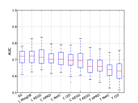
B

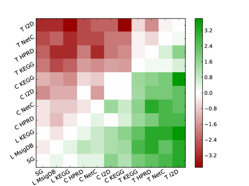
Figure 1: Performances of the NMCs employing single genes and composite features constructed from different secondary data sources. For each combination of feature extraction method and secondary data source and each pair of data sets we obtained one AUC value resulting in 30 AUC values per combination. The number of features for each classifier was determined in the cross-validation procedure (CV-optimized). A: Each box plot shows the median, the $25\%$ and $75\%$ percentiles and the standard deviation of the 30 AUC values. Outliers are depicted by crosses. The boxes are sorted in descending order according to the median. B: This panel shows the result of pairwise comparisons between all combinations of feature extraction methods and secondary data sources. If, for a given combination of training and test data set, the AUC value of classifier $i$ is higher (lower) than the AUC value of classifier $j$ on the same test data set, it is counted as a win (loss) for classifier $i$. Element $(i,j)$ in the matrix represents the $\log_{2}$ ratio of wins to losses of method $i$ compared to method $j$. Green indicates an overall win, red an overall loss and white represents draws. The rows and columns are sorted as in Panel A. Abbreviations: SG: Single genes; C: Chuang; L: Lee and T: Taylor.

Four hypotheses regarding the lack of observed performance differences

Next we formulated a number of hypotheses that could explain why classifiers employing secondary data sources do not outperform single gene classifiers. These hypotheses relate to (1) the feature selection approach employed; (2) the starting set of genes employed in each of the approaches; (3) the effect of the training set size on performance and (4) the homogeneity of the data set employed. In the following sections we will investigate these hypotheses one by one.

The number of selected features does not effect relative performances

In the cross-validation protocol that we proposed for unbiased performance evaluation and also employed in the comparison, we employ individual feature filtering to select an optimized number of features to employ in the classifier. While this approach is sub-optimal, we (Wessels et al. [11]) and others have shown that these simple approaches perform the best in predicting phenotypes based on gene expression data. However, we observed in the curves showing the AUC values as a function of the number of ranked features included in the classifier (Figures S2-S4) that the AUC values for the NMC are very stable across a large range of features for most approaches, and that the absolute maximal AUC value chosen during the feature selection routine might only marginally differ from the performance obtained with other feature values. For this reason, and since the selection of the optimized number of features introduces additional variability between the approaches, we decided to fix the number of features to 50, 100 and 150 for most approaches. We chose these values as they covered the feature ranges across which the performance remained stable in all approaches. The results for fixing the number of features to 50 are depicted in Figure 2 while results for 100 and 150 features are presented in Figures S5 and S6. When accounting for multiple testing, no classifier using a fixed number of features performs significantly different from its counterpart using the number of features determined by cross-validation. See p-values of the pairwise Wilcoxon rank test in Tables S4, S6 and S8. As expected, there are only minor differences between the performance of classifiers when the number of features is restricted to 50, 100 and 150 (Tables S3, S5 and S7) with any significant differences favoring single genes. This confirms that the number of features is not a critical parameter. Based on these results, we can conclude that the number of selected features does not explain the observed differences between composite feature classifiers and single gene classifiers.

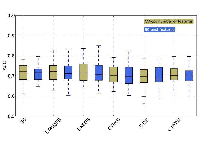
Figure 2: Performance of all classifiers restricted to 50 features. Comparison of the performance of the classifiers when the number of features is trained in the CV procedure (denoted as ‘CV-opt number of features’, same values as in Figure 1) and when the 50 best scoring features (denoted as ‘50 best features’) are selected for classification. We cannot show the values for Chuang-KEGG, Taylor-KEGG or Taylor-HPRD since for some data sets, the number of significant composite features was lower than 50. Abbreviations of methods as in Figure 1.

Restricted gene sets are not detrimental to composite feature classifiers

We next hypothesized that the lack of difference in the performance between composite classifiers and single gene classifiers could be caused by the fact that the composite features are bound to the genes annotated in the secondary data while single gene classifiers can employ all genes on the microarray. To test this hypothesis we retrained the single gene classifier, but restricted the set of genes from which features for the final classifier could be selected to the genes that are present in the respective secondary data sources. The resulting classifiers are denoted by the secondary data source from which the gene set is derived, while the single gene classifier employing features from the whole microarray is denoted by unrestr. The results of this analysis are depicted in Figure 3A. There is significant difference in the performance of the classifiers employing genes annotated in the I2D, KEGG and MsigDB (Table S9). However, when accounting for multiple testing only the difference between unrestr and I2D remains significant. Moreover, as indicated earlier, the optimization of the number of features by cross-validation introduces significant variation in the number of features without resulting in large performance changes. To eliminate this source of variation from the comparison, we fixed, as before, the number of features to 50, 100 and 150 and repeated the comparisons. The results are depicted in Figures 3B and S7, and Tables S10-S12. We can only find significant differences between the unrestricted single gene classifier and KEGG when the 50 best features are selected and the I2D when employing the 150 best features. However, both of these differences disappear when multiple testing correction is performed. We therefore conclude that the starting gene set has a minor influence on the single gene classifiers. Hence we can reject the hypothesis that feature extraction approaches employing secondary data sources are put at a disadvantage since they can not exploit the full set of genes present on the array.

A

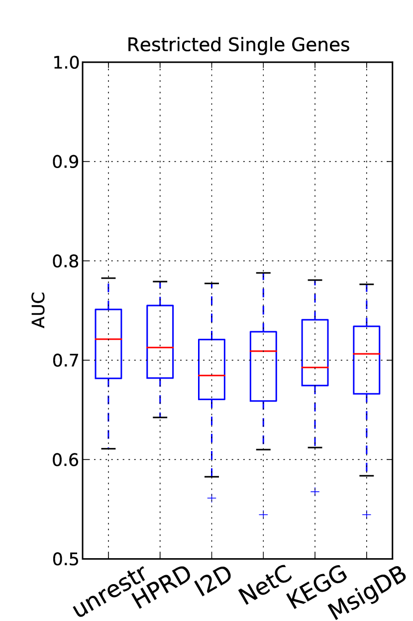
B

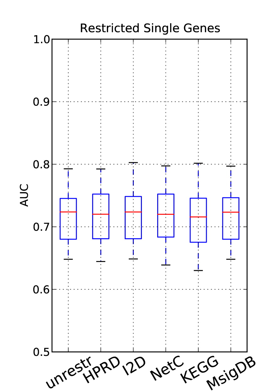
Figure 3: Comparison of single gene classifiers restricted to genes occurring in the secondary data sources. We compared the performance of the single gene classifier trained on all genes present on the microarray (unrestr.) with the performance of single gene classifiers that only employ genes present in the secondary data sources. The resulting classifiers are indicated by the secondary data source whose gene set was employed to train the classifier. A: The number of single genes was determined during the cross-validation procedure; B: the 50 best scoring single genes were employed.

Training set size has no significant effect on performance differences

A third possible factor that could explain the lack of performance difference between the composite feature classifiers and the single gene classifier is the size of the training set. Recall that in the cross-validation procedure we train on one data set and then test on another data set. We repeat this procedure for all possible pairs of data sets; excluding, of course, training and testing on the same data set (paired setting). We can, however, also follow an alternative scheme where we train on all data sets except the test set, the so-called merged setting. More specifically, in this setting four of the five Affymetrix data sets were merged to form a single training data set and the fifth data set was used as test set. Thus, we receive for each feature selection method five AUC values. This increases the size of the training set, and by comparing the results obtained in this setting with the results from the paired setting, we can investigate the effect of the training set size on the classifier performances.

Figure 4 depicts the results for the merged setting and the pairwise setting for the CV-optimized feature sets and when only the top 50 features are selected. (Note that, in contrast to the results in Figure 1, this pairwise setting only employs the Affymetrix datasets). The results for the top 100 and 150 features are similar, see Figure S8. Statistical testing shows that in the paired setting (Tables S13-S16) when the number of features is set to 150, Lee employing the MsigDB performs better than the single gene classifier. However, this difference disappears when correcting for multiple testing. More importantly, there are no significant differences between the performances of the single gene and composite feature classifiers in the merged setting (Tables S17-S20).

Hence, we can also reject the hypothesis that the lack of performance difference is due to the sizes of the employed training sets.

	CV-opt features	50 best features
merged
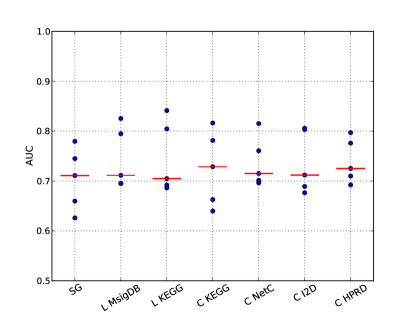
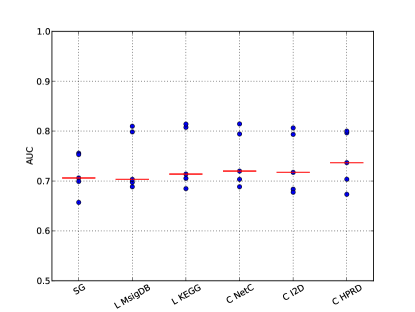
pairwise

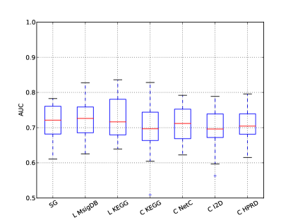
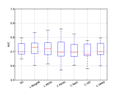
Figure 4: Classification results for merged and paired setting. In the merged setting one Affymetrix data set is set aside as test and the remaining four Affymetrix data sets are merged into a single data set. This is repeated until every one of the five data sets acted as a test set. Top row: Results for the merged setting. The red lines indicate the median. Bottom row: Only the five Affymetrix data sets were used in the paired setting.

Dataset homogeneity affects single genes and composite classifiers similarly

Breast cancer is a collection of several heterogeneous diseases that show very different gene expression patterns [17]. Expression patterns predictive of outcome might vary between subtypes, which typically leads to problems when training classifiers on gene expression data derived from breast tumors. If this is not explicitly taken into account during classifier training it could result in poor performance and unstable classification, as the selected genes may depend on the composition of the training set. In this section we control the heterogeneity in both the training and test sets by only selecting the relatively homogeneous ER positive breast cancer sub-population. Since the training sets become too small in the paired setting if we only select the ER positive cases, we followed the merged setting outlined above. More specifically, we created a test set consisting of all ER positive cases of a single data set and a training set by pooling all ER positive cases from the remaining data sets. We repeated this procedure across the six data sets and thus obtained six AUC values per classifier. Figure 5 depicts the results for the CV-optimized feature sets and the top 50 features. As before, the classifiers employing a fixed number of features perform similar to classifiers based on a feature set optimized in the CV procedure. See Figure 5B and Figure S9. In general, and in accordance with earlier observations as made, e.g., by Popovici et al. [10], the performance of all classifiers is substantially better on the ER positive cases compared to the unstratified case. More importantly, also in this setting there are no significant performance differences between the single gene classifiers and composite feature classifiers (Tables S21-S24).

A

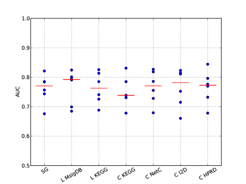
B

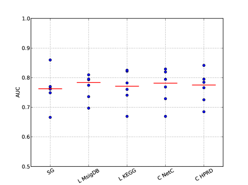
Figure 5: Classification results of the ER positive data only. The ER positive cases from a single data set were set aside as test set while ER positive cases from the remaining five data sets were merged into a single training set. This was repeated until each data set was employed as left-out test set, resulting in six AUC values. The red lines indicate the median. A: CV-optimized number of features; B: 50 best features.

Equal classification using real or randomized networks and pathways

In the previous sections we showed that composite classifiers do not perform significantly better than classifiers employing single genes as features. We investigated several factors that could influence the performances of these two approaches, but failed to find any factor that induces significant performance differences on the data sets we employ in this study. This lead us to question whether prior knowledge sources really contain information that is of value in constructing features for classifiers predicting outcome in breast cancer. Chuang et al. [3] compared their PPI-based classifier to classifiers derived from randomized PPI networks. They concluded that their classifier performed significantly better than random classifiers. We decided to repeat this analysis for a subset of the classifiers in our comparison to determine whether prior knowledge sources really contain information relevant for predicting outcome in breast cancer. To this end, we generated, for each prior knowledge source, 25 random instances. More specifically, we maintained the structure of the pathways, networks and gene sets, and randomly permuted the identities of the genes. In doing so, the original topology of the secondary data is preserved while the biological information is destroyed. We then repeated the whole validation procedure on all 25 random instances for the feature extraction methods Lee and Chuang. The results of this analysis are presented in Figure 6. Strikingly, classifiers derived from secondary data sources suffer no significant performance degradation when employing randomized secondary data sources. The performance of Chuang on randomized PPI data clearly has a large variance, and there are instances of classifiers derived from random networks that perform much worse and much better than classifiers derived from the non-randomized networks. Furthermore, we found that most classifiers based on randomized secondary data show performances similar to the classifiers derived from the real secondary sources. To formalize this observation, we performed a statistical test. We have reason to believe that the results derived from the real data should be better than the results derived from random data. Hence we performed one-sided paired Wilcoxon rank tests to determine whether the null hypothesis that the mean ‘real’ AUC-value is larger than each of the the 25 ‘randomized’ mean AUC-values can be rejected. We performed a Bonferroni correction to account for multiple testing. The results in Figures S10-S12 and Tables S25-S30 show that in the vast majority of the cases the null hypothesis can not be rejected. Conversely, it is very simple to generate a randomized secondary data source that performs equally well as the real data source. This result shows that further research must be done on the utility of secondary data sources in predicting breast cancer outcome.

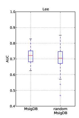
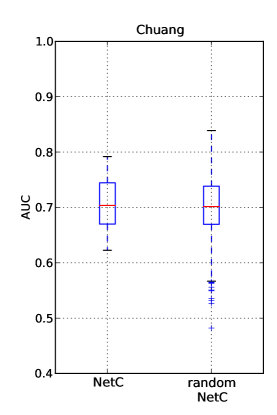
Figure 6: The effect of randomized secondary data sources. Left: AUC values obtained with the feature extraction method Lee on real and randomized MsigDB pathways. Right: AUC values obtained with the feature extraction method Chuang on real and randomized PPI networks.

Current composite feature classifiers do not increase the stability of gene markers

Apart from performance improvements, it is also frequently claimed that features derived from classifiers employing secondary data sources are far more stable than single gene classifiers. In other words, whereas single gene signatures extracted from different data sets show very little overlap, features extracted by approaches that employ secondary data sources are claimed to show a large degree of overlap, even though the features were derived from separate data sets.

In this section we determined whether feature sets extracted from secondary data sources do, in fact, show a larger degree of stability than single gene feature sets. As a measure of stability we calculated the pairwise Jaccard index between the features derived from different data sets for a given feature extraction method. Since the number of features determined in the CV procedure varies, we performed this comparison for the cases where the top 50, 100 and 150 features are selected. The Jaccard indices for the best 50 features are depicted in Figures 7 while Figure S13 depicts the results for the best 100 and 150 features. It is clear that the overlap of feature sets consisting of single genes is relatively low, albeit slightly higher than the overlap of Lee-MsigDB. The highest consistent stability is obtained by Chuang-HPRD with Chuang-KEGG showing high variance in stability. One can therefore clearly conclude that, when compared in terms of signature genes overlap, single genes are generally less stable than feature sets extracted by including secondary data sources. However, strictly speaking, such a comparison compares the proverbial apples and oranges, since a single feature constructed based on secondary data sources can contain many genes. In order to ensure that the low overlap of single genes is not only due to the fact that the best single gene feature sets contain fewer genes than the other feature sets, we controlled the single gene feature sets for size. More specifically, for each data set and each feature selection approach employing secondary data sources, we obtain a single best feature set consisting of $n^{*}$ features (networks, gene sets or pathways) that, in turn, consists of $m$ genes. We then determine a size-matched single gene set by choosing the best $m$ single genes on that same expression data set. We also required these single genes to be annotated in the respective secondary data source. For these size-matched single gene feature sets, we computed the Jaccard index. The results, depicted in Figure 8 and S14, show that when this size correction is applied, the stability of single gene feature sets are as high as features extracted by employing secondary data sources. See also Tables S31-S33.

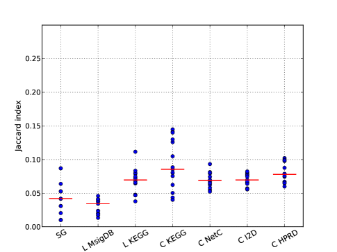
Figure 7: Feature stability when the top 50 features are selected. For each method the Jaccard index was calculated between the gene sets extracted from two different data sets. This was repeated for all pairwise combinations of data sets. Thus, 15 values were obtained.

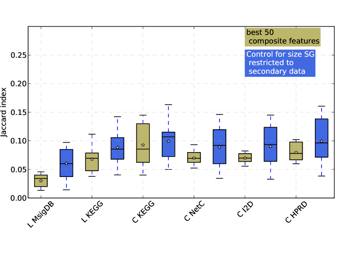
Figure 8: Feature stability when corrected for gene set size. Box plots of the Jaccard indices computed for all pairs of gene sets derived from two different data sets. The green box plots represent the Jaccard indices for genes constituting composite features, while the blue box plots (denoted as ‘Control for size SG’) represent the gene-size-corrected Jaccard indices for single gene classifiers. The white stars represent the mean of the distributions.

Discussion

In this study we evaluated the prediction performance of network and pathway-based features on six breast cancer data sets. In contrast to previous studies we found that none of the classifiers employing composite features derived from secondary data sources can outperform a simple single gene classifier. Moreover, we did not find any evidence that composite features show a higher stability across the six breast cancer cohorts. Our findings suggest that with the feature extraction methods tested in this study, we cannot extract more knowledge from secondary data sources than we find in the expression of single genes.

There are several issues that could potentially contribute to that situation. First, secondary data sources are, to a large degree, generated by high-throughput biological experiments and could thus contain a level of noise that deems them inappropriate for outcome prediction in breast cancer. On the other hand, the search algorithms could be unsuitable to detect biologically meaningful networks. All three feature extraction methods only extract local information without taking into account the full structure of the network or pathway data. This local information is then combined in the classifiers in a rather crude way, namely by simply averaging the expression of the genes associated with a feature that was found to be associated with outcome, i.e. treating each single sub-network or sub-pathway as a single dimension in the classification space. Possible dependencies between features are not taken into account. Also, exploring the subnetwork search space in a heuristic manner may decrease classification performance. The recent method by Dittrich et al. [18] computes provably maximally deregulated connected subnetworks based on a sound statistical score definition. This method has not yet been used for classification.

Other recent algorithms as presented by Ulitsky et al. [19], Chowdhury et al. [20] and Dao et al. [21] search for deregulated subnetworks in subsets of samples. These subnetworks are sets of genes that are deregulated in most, but not necessarily all, patients with poor disease outcome. The heuristic method by Chowdhury et al. [20] has been shown to perform well on cross-platform classification of colorectal cancer outcome. Dao et al. [21] improved on these results by exact enumeration of all dense subnetworks with the above-mentioned property. Looking at subsets of samples in a class, i.e. a subset of the poor outcome samples, is an interesting aspect for further evaluation, in particular for breast cancer outcome prediction as it may quite accurately capture the large phenotypic variety of this rather inhomogeneous disease.

Lee et al. [4] and Chuang et al. [3] average the expression values of single genes comprising a subnetwork, to determine the ‘activity’ of the subnetwork. This is, however, a very simplistic view of the dynamics in a subnetwork itself. In contrast to these two algorithms, the method by Taylor et al. [5] predicts outcome by trying to capture the disruption of the regulation of a hub protein over its interactors in poor outcome patients. This is implemented by using every edge leading to a hub as a feature in classification space. Yet, in this way, the classification space becomes too large to allow for good classification results. This method is thus not appropriate for solving the classification problem and this is clearly demonstrated in the poor performance of this algorithm in the comparison.

To find a subnetwork scoring function remains one of the biggest problems when including promising gene sets into a classification framework. Abraham et al. [7] tested the classification performance of gene sets provided by the MsigDB. The authors employed several set statistics like mean, median and first principle component to score the gene sets. They found that none of the classifiers employing gene sets and scoring them with the set statistics performed better than a single gene classifier.

In our experiments where we shuffle the genes in the secondary data we showed that features determined on this nonsensical biological data perform equally well in classification than features determined on the real secondary data. This again could possibly be caused by the low quality of the network and pathway data. However, the nature of gene expression patterns in breast cancer, and specifically its association with outcome can also explain these findings. Since many genes are involved in breast cancer and are differentially expressed and associated with outcome, as shown, for example by Ein-Dor et al. [22], the chance that those genes span decently sized subnetworks in the randomized secondary data is high. Both algorithms, Chuang and Lee, look for highly differentially expressed subnetwork or pathway markers, and these can also be found in the randomized data. Furthermore, overlaying networks or pathways that contain protein level information with mRNA expression data might result in erroneous results. These data sources reflect events on very different molecular levels. While gene expression and protein expression is undoubtedly linked, there are many processes that prevent this from being a trivial one-to-one mapping. Thus, we may measure, for a set of genes, an effect on the mRNA level that leads to differential expression between the two patient classes but this may have little bearing on the relationships between these genes as captured in the PPI graph. In conclusion, our results show that it may not be sufficient to search for sub-networks or sub-pathways that are differentially expressed on average but that complex interactions between entities as well as the more complicated relationships between mRNA levels and the topology of the PPI graph need to be taken into account.

Our different classification results are partially owed to the fact that we used a different cross-validation procedure, which, in our opinion, fits the clinical situation, better. The studies by Chuang et al. [3] and Lee et al. [4] also determined possible features on one data set. However, in contrast to our work they reranked the features on the second (test) data set. Furthermore, they determined the number of features and the classification performance on this second data set using five-fold cross-validation. In our opinion, this does not represent a bona fide independent validation of the classifier.

In summary, we introduced a framework to test the use of feature extraction methods with respect to the prediction of their determined features. We used this framework to specifically test the superiority of feature extraction methods based on network and pathway data over classifiers employing single genes. Across six breast cancer cohorts, we showed that the three tested methods do not outperform the single gene classifier nor do they provide more stable gene signatures for breast cancer.

An important aspect that hampers progress in the field of network and pathway based classification is the lack of proper evaluation of proposed algorithms. In our opinion this is caused by (1) lack of reproducibility of the results; (2) lack of large and standardized benchmark sets to test proposed algorithms and (3) lack of a standardized, unbiased protocol to assess the performances of proposed methods on the benchmark sets. To overcome these issues, we have created a software pipeline that implements all the classifiers as faithfully as possible and also runs our validation protocol. We have also established a large collection of breast cancer datasets (and this is currently being expanded) on which the algorithms can be tested. Both the datasets and the pipeline are freely available. In the long term, we envision a web service where a classifier can be submitted as a software package. The server will then autonomously evaluate the performance of the classifier using the standardized pipeline on the benchmark set.

Materials and Methods

Microarray data

The microarray data sets used in this work is listed in Table 2. To combine the five Affymetrix arrays with the Agilent arrays we first matched the probes on the arrays to Entrez GeneIDs. Only those genes were included in the feature sets that appeared on both platforms, resulting in 11601 genes in total. In case that several probes on one chip matched to the same gene the expression values of the probe with the highest variance was taken. The final expression matrices were then z-normalized such that the expression distribution of each gene has a mean of zero and a standard deviation of one. Samples in the data sets were labeled ‘good’ outcome if no event, that is, a distant metastasis or death, occurred within five years. Otherwise samples were labeled ‘poor’ outcome.

Table 2: Microarray expression data

Dataset	Outcome	poor/good	platform
Chin [23]	Metastasis within 5 years	68/29	Affymetrix
Desmedt [24]	Metastasis within 5 years	91/29	Affymetrix
Loi [25]	Metastasis within 5 years	92/28	Affymetrix
Miller [26]	Death within 5 years	156/37	Affymetrix
Pawitan [27]	Death within 5 years	120/22	Affymetrix
Vijver [13]	Metastasis within 5 years	178/70	Agilent

Expression data used in this study. All data sets were processed as described in [28] and contained 11601 genes with z-normalized expression values afterwards. Column ‘poor/good’ contains the number of samples with poor or good outcome, respectively.

ER status of patients was predicted from the expression values of the gene ESR1. For more detail of the processing of the data see van Vliet et al. [28].

Network and pathway data

All feature extraction methods were run on the databases KEGG [14] and HPRD [29]. The algorithm by Lee et al. [4] was also run on the MsigDB C2 database [9].

KEGG

We collected all pathway information available for Homo sapiens (hsa) from the KEGG database, version December 2010. The entries contained information on metabolic pathways, pathways involved in genetic information processing, signal transduction in environmental information processing, cellular processes and pathways active in human disease and drug development. We obtained 215 pathways. The nodes contained in the pathways were matched with the KEGG gene database such that each node carries an Entrez GeneID. In this way we obtained a network composed of 200 pathways containing 4066 nodes and 29972 interactions of which 3110 nodes are also contained in the expression sets.

MsigDB

As second pathway database we used the C2 collection of the MsigDB (version 3) [9], which was also used in Lee et al. [4] (version 1.0). It contains gene sets from online pathway databases such as KEGG, gene sets made available in scientific publications and expert knowledge. We obtained 3272 gene sets of which 2714 could be entirely or partially mapped the six data sets. The MsigDB does not contain any edges, thus this database was only usable for the algorithm by Lee et al. [4].

HPRD

The HPRD (version 9) provides information on protein-protein interactions (PPI) derived from the literature. The HPRD contains 9231 proteins and 35853 interactions. The proteins were mapped to their genes carrying Entrez GeneIDs. There are 7390 genes contained in both the HPRD and the expression sets.

OPHID/I2D

The OPHID/I2D database, downloaded in April 2011, contains protein-protein interactions derived from BIND, HPRD and MINT as well as predicted interactions from yeast, mouse and C. elegans. The database contains 12643 nodes and 142309 edges. 9453 of the nodes are also present in the six breast cancer studies examined here.

Protein-protein interaction network by Chuang et al. [3] (NetC)

The network curated by Chuang et al. [3] consists of 57228 interactions and 11203 nodes of which 8572 are contained in the six breast cancer studies. The network is curated from yeast two hybrid experiments and interactions predicted from co-citation.

Algorithms

Notation

Let $E_{k\times n}$ be a gene expression matrix, as we obtain it from a microarray study, with $k$ samples and $n$ genes. Each entry $e_{i,j}$ contains the expression value of gene $j$ in sample $i$. All samples carry a binary class label $l_{i}\in\{0,1\}$ denoting outcome, where 1 denotes ‘poor outcome’ and 0 denotes good outcome’. The label vector of all samples is denoted by $L=(l_{1},\dots l_{k})^{T}$. We denote a network by $N=(G,I)$ where $G$ is the set of genes in the network and $I$ is the set of interactions between these genes, also called edges in the following. We define a subnetwork as the connected graph $N^{\prime}=(G^{\prime},I^{\prime})$ with $G^{\prime}\subseteq G$ and $I^{\prime}\subseteq I$, and a pathway as a gene set $G^{\prime}\subseteq G$. Let $G^{\prime}$ be such a pathway or the set of genes in a subnetwork then according to [3, 4] the activity of the pathway or subnetwork in sample $i$ is given as

$$a_{G^{\prime},i}=\sum_{j\in G^{\prime}}\frac{e_{i,j}}{\sqrt{|G^{\prime}|}}$$ (1)

Feature extraction method by Chuang et al. [3]

Given a network $N=(G,I)$, the algorithm by Chuang et al. [3] carries out a greedy search starting from a seed—a single gene in the network. It then iteratively extends the network by adding neighboring genes to find subnetworks with high mutual information (MI) of the activity of the pathway and sample labels. Each node in $N$ is used once as seed. In each step, an additional gene is picked that leads to a maximal MI improvement. If no improvement is possible, the search stops.

More precisely, the association between the subnetwork activity and the class labels is computed as follows: Given a subnetwork $N^{\prime}=(G^{\prime},I^{\prime})$ the activity vector $a_{G^{\prime}}=(a_{G^{\prime},1},\dots,a_{G^{\prime},k})^{T}$ is calculated using Equation (1). To compute the MI, vector $a_{G^{\prime}}$ is discretized. Given a dissection of the interval $[\min_{i\in[1,\dots,k]}a_{G^{\prime},i},\max_{i\in[1,\dots,k]}a_{G^{\prime},i}]$ into $\lceil\log_{2}k\rceil$ bins let $\delta:\mathbb{R}\rightarrow[\delta_{1},\dots,\delta_{\lceil\log_{2}k\rceil}]$ be a function that assigns a network activity to a sample with one of these bins, where $\delta_{i}$, $i=1,\dots,\lceil\log_{2}k\rceil$, denote the bins. We define the mutual information $s_{\mathit{MI}}$ between the probability density of the bins $p(\delta(\cdot))$ and the probability distribution of the class labels $p(l)$ as

$$s_{MI}(\delta,l)=\sum_{i=1}^{\lceil\log k\rceil}\sum_{l=0}^{1}p(\delta_{i},l)\log\frac{p(\delta_{i},l)}{p(\delta_{i})p(l)}$$ (2)

where $p(\delta_{i},l)$ is the joint distribution of $p(\delta(\cdot))$ and $p(l)$. The algorithm also performs three statistical tests to extract only networks that show significantly high mutual information. The ranking of the networks is given by ordering the networks according to their mutual information $s_{\mathit{MI}}$.

In our study we use PinnacleZ, an implementation of the algorithm provided by the authors. As feature values for classification the subnetwork activity as given in Equation (1) of the determined subnetworks was used.

Before determining the subnetworks, PinnacleZ performs a z-normalization of the given data set. This is undesirable when looking at subsets of data sets as we do in the five-fold cross-validation. In order to skip the normalization step, we implemented a patch in the PinnacleZ source code. This patch adds a “-z” option that instructs PinnacleZ to omit its usual gene-wise z-normalization step.

One problem when mapping the expression data to the network data is that for some nodes there is no expression data. Chuang et al. [3] do not state in their paper how they handled this problem although their identified subnetworks contain such nodes. We therefore filtered out proteins for which no expression data is available before running PinnacleZ. For further issues we encountered when working with PinnacleZ see the supplementary information.

Algorithm by Lee et al. [4]

The algorithm by Lee et al. [4] uses the t-statistic to rank pathways according to their overall differential expression. For this it first defines sets of genes, the so called condition responsive genes (CORGs), which contain the most differentially expressed genes of a pathway. These genes are found by applying a greedy search. For each pathway the genes are ordered according to their t-statistics. Given the two sample groups let $E^{1}_{j}$ be the expression values of gene $j$ for all samples with class label $1$ and $E^{0}_{j}$ the expression values of gene $j$ for all samples with class label $0$, respectively. Let $k^{0}$ and $k^{1}$ denote the number of samples in each group; $\mu_{E^{0}_{j}}$ and $\mu_{E^{1}_{j}}$ denote the means of the two groups and $\sigma_{E^{0}_{j}}$ and $\sigma_{E^{1}_{j}}$ the standard deviation in the two groups. The t-statistics between $E^{1}_{j}$ and $E^{0}_{j}$ is given by

$$t(j)=\frac{\mu_{E^{1}_{j}}-\mu_{E^{0}_{j}}}{\sqrt{\sigma_{E^{1}_{j}}/k^{1}+\sigma_{E^{0}_{j}}/k^{0}}}$$ (3)

The genes in a pathway are sorted either in ascending order, if the highest absolute $t$ value is negative, or in descending order, if the highest absolute $t$ value is positive. Given this order the greedy search iteratively combines genes and calculates their average expression, or pathway activity, across the samples as it is given in Equation (1), i.e. $a_{G^{\prime}}=(a_{G^{\prime},1},\dots,a_{G^{\prime},k})^{T}$ is calculated where $G^{\prime}$ contains the best $m$ genes according to the ranking. To evaluate the combined discriminative power of the genes that have been averaged, the t-statistic of the averaged expression is computed as follows:

$$s_{G^{\prime}}=t(G^{\prime})=\frac{\mu_{a^{1}_{G^{\prime}}}-\mu_{a^{0}_{G^{\prime}}}}{\sqrt{\sigma_{a^{1}_{G^{\prime}}}/k^{1}+\sigma_{a^{0}_{G^{\prime}}}/k^{0}}}$$ (4)

where $\mu_{a^{0}_{G^{\prime}}}$ and $\mu_{a^{1}_{G^{\prime}}}$ represent the means and $\sigma_{a^{0}_{G^{\prime}}}$ and $\sigma_{a^{1}_{G^{\prime}}}$ represent the standard deviations of the averaged activities. If the resulting value $t(G^{\prime})$ is higher than the previous value of the t-statistics then the search continues adding the gene to the already determined CORGs, otherwise the search stops. The score $s_{G^{\prime}}$ of the final CORGs $G^{\prime}$ is then used to rank the pathway.

As mentioned beforehand, Lee can only be executed on predefined gene sets. Those gene sets are normally not provided in a PPI database. Thus, we used the KEGG and MsigDB databases to evaluate this algorithm. In order to decrease the running time the authors executed a pathway ranking by employing the algorithm by Tian et al. [30] and just taking the top 10% of pathways into account prior to executing their algorithm. In our setting we ranked all of the pathways according to the algorithm by Lee et al. [4] and considered for determining the optimized number of features in the final classifier all pathways in KEGG and the top 400 pathways in MsigDB. As feature values for classification the pathway activity, as computed according to Equation (1) for all condition-responsive genes (CORGs), is employed. Here again we excluded proteins in the pathways for which no expression data is available.

Algorithm by Taylor et al. [5]

In contrast to the algorithms by Chuang et al. [3] and Lee et al. [4], the algorithm by Taylor et al. [5] first identifies organizer proteins in the network, the so-called hubs, and then attaches a weight to each edge between the hubs and their direct neighbors in the network. These weights are later used to train a classifier.

Candidate hubs are the 15% most densely connected proteins in the network data, independent from their expression status. For the following calculations proteins without expression data are excluded. To identify hubs that significantly change their interaction behaviour between the two classes the authors introduce the hub difference and the average hub difference which are based on the Pearson correlation. The Pearson correlation between a hub $h$ and an interactor $n$ of this hub is defined as the Pearson correlation between their expression profiles across the $k$ samples

$$P(h,n)=\frac{\sum^{k}_{i=1}(e_{n,i}-\mu_{E_{n}})(e_{i,h}-\mu_{E_{h}})}{(k-1)\sigma_{E_{n}}\sigma_{E_{h}}}\enspace.$$ (5)

$E_{n}$ and $E_{h}$ denote the distribution of expression values across the $k$ samples and $\mu$ and $\sigma$ are their means and standard deviations. The hub difference is defined as the difference of the Pearson correlation $P(h,n)$ given the two sample classes, indicated by the superscript $0$ and $1$,

$$\mathit{d}(h,n)=P^{0}(h,n)-P^{1}(h,n)\enspace.$$ (6)

Let $\delta(h)$ denote the set of neighbors of a hub $h$ then the average hub difference is

$$\mathit{\overline{d}}(h)=\frac{\sum_{n\in\delta(h)}|\mathit{d}(h,n)|}{|\delta(h)|}\enspace.$$ (7)

To extract only those hubs that show a significant average hub difference the value is compared to a distribution of the average hub difference for a permuted dataset, using a p-value cut off of $0.05$. This distribution is calculated by 1) randomly permuting the class labels and 2) recalculating the average hub difference and repeating these two steps 1000 times. The significant hubs are ranked by their average hub difference.

As feature values in the classifier differences of the expression of the hub and each of its interactors were used. For example, suppose $h_{1},\dots,h_{p}$ were found significant and suppose ${(h_{1},i_{1,1}),\dots,(h_{1},i_{1,m_{1}}),\dots,(h_{p},i_{p,1}),\dots,(h_{p},i_{p,m_{p}})}$ are the edges to their interactors. Then for one sample the vector $(e_{h_{1}}-e_{i_{1,1}},\dots,e_{h_{1}}-e_{i_{1,m_{1}}},\dots,e_{h_{p}}-e_{i_{p,1}},\dots,e_{h_{p}}-e_{i_{p,m_{p}}})$ contains the feature values for the classifier.

Since the edges attached to a hub are not ranked, all those edges were included in the classifier, given that the hub shows a significant average hub difference. For the cross-validation procedure this means that we can not train the number of features but only a number of feature sets.

Classifiers

In our study we employed a nearest mean classifier (NMC) and logistic regression (LOG). As distance metric for the NMC we employed the Euclidean distance. More specifically, a sample is projected on the line connecting the two class means, and the Euclidean distance of he projected sample to each class mean is computed. The sample is assigned to the closest class.

In addition to the NMC we executed all features extraction methods in combination with the LOG. We found that simple LOG without any regularization parameters cannot be trained properly since for higher numbers of features (approximately 50 features and more) the training step does not converge on the breast cancer data. Moreover, we found that for many features different implementations of LOG return different weight vectors. Thus, we used three different implementations (the R GLM, R NNET and Python SciKits implementation) and only accepted the classification result of the R GLM implementation when all three versions converged to the same weight vector.

Cross-validation and classification

In the cross-validation procedure we employed, we rigorously separate the training and test data sets. For details, see Figure 9 and Algorithm 1. The training phase consists of determining the best performing number of features and training the final classifier with this number of features. The trained classifier is then tested in the test phase. The data sets used in these two phases are completely independent, i.e. the test set is never used in training the classifier.

To determine the optimized number of features in our classifiers we employed five fold cross-validation. In this cross-validation, we first determined all required composite features (if necessary) and their ranking on four splits of the training data set. Then a series of classifiers is trained on the same four splits by gradually adding features according to the ranking. These classifiers are then evaluated on the fifth split of the data set. Since this is done in a five fold cross-validation we obtain for each of the classifiers five different AUC values. The optimized number of features extracted corresponds to the number of features yielding the highest mean performance. Once the best performing number of features is determined, the features are calculated using the whole training data set and the final classifier is trained also using the complete training data set. The classifier is then tested on the test data set. For each method we used all possible pairs of data sets as training and test set respectively. Since we have six data sets available this resulted in 30 AUC values for each method.

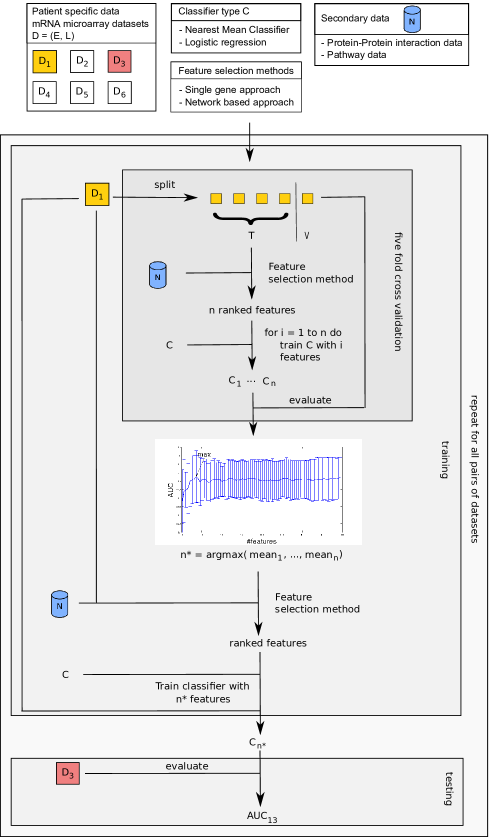
Figure 9: Overview of validation procedure. Input: patient-specific mRNA expression data $D=(E,L)$ where $E$ is an expression matrix and $L$ a vector with class labels; an untrained classifier; a feature extraction method and an additional secondary data source $N$ is used in the feature extraction method. Five fold cross-validation is used to determine the best performing number of features in the final classifier. The data set $D_{1}$ is split into five parts of which four parts are used as training set $T$ and one part is used as test or validation set $V$. First $T$ is used to extract features and to rank them. A series of classifiers is then trained, where the number of features is gradually increased by adding features according to the ranking. All classifiers are evaluated using $V$. As performance measure the area under the curve (AUC) is used. At the end of the cross-validation each of the five splits has been used for validation once, thus we obtain five different AUC values. We choose the number of features $n^{*}$ in the final classifier to be the number of features corresponding to the highest mean AUC value. The best $n^{*}$ features are determined on the whole data set $D_{1}$ and the final classifier with these features is also trained on $D_{1}$. This classifier is then tested on a different data set $D_{3}$. We evaluated all possible pairs of data sets ($\{(D_{1},D_{2}),\dots,(D_{1},D_{6}),(D_{2},D_{1}),\dots,(D_{6},D_{5})\}$) to evaluate each feature extraction method in a certain setting resulting in 30 AUC values for each setting. These values were then analyzed in a box plot or a winchart. The features in the six classifiers ($C_{n^{*}}$ of each data set) were used to determine the stability of gene markers across different data sets.

Algorithm 1 Cross-validation procedure

0:  Datasets $D_{1}=(E_{1},L_{1})$, $D_{2}=(E_{2},L_{2})$ where $E_{1},E_{2}$ are expression matrices and $L_{1},L_{2}$ are vectors of outcome labels Feature extraction method $m\in\{$SG, L, C, T$\}$Secondary data source $N$Classifier $C\in$ {logistic regression, nearest mean classifier} /* Cross-validation on $D_{1}$ */

1:  $(d_{1},d_{2},d_{3},d_{4},d_{5})\leftarrow D_{1}$ /* split samples in $D_{1}$ into $5$ parts $d_{k}=(e_{k},l_{k})$ where $e_{k}$ denotes the expression values of the samples in split $k$ and $l_{k}$ their class labels */

2:  for $s\leftarrow 1$ to $5$ do

3:     $\mathit{Val}\leftarrow d_{s}$ /* validation set $(e_{\mathit{val}},l_{\mathit{val}})$ */

4:     $\mathit{Train}\leftarrow D_{1}\setminus d_{s}$ /* training set $e_{\mathit{train}},l_{\mathit{train}}$ */

5:     $\mathit{rankedF}\leftarrow m(\mathit{Train},N)$ /* determine features according to the published methods and rank them according to the appropriate score or determine the ranking of the single genes according to the t-statistic on $\mathit{Train}$ */

6:     $n\leftarrow$ number of $\mathit{rankedF}$

7:     $\mathit{AUC}_{s}$ = empty list

8:     for $i\leftarrow 1$ to $n$ do

9:        $C_{s,i}\leftarrow\mathit{trainCl}(C,\mathit{rankedF}[1,\dots,i],\mathit{Train})$ /* train the classifier with $i$ features */

10:        $\hat{p}\leftarrow C_{s,i}(e_{\mathit{Val}})$ /* ranking of the samples in the validation set */

11:        $\mathit{AUC}_{s,i}\leftarrow\mathit{calcAUC}(\hat{p},l_{\mathit{Val}})$ /* calculate AUC value for $C_{s,i}$ */

12:     end for

13:  end for/* train CV-optimized classifier on $D_{1}$ and validate it on an independent data set $D_{2}$ */

14:  for $j\leftarrow 1$ to n  do

15:     $\mathit{meanAUC}[j]\leftarrow mean(\mathit{AUC}_{1}[j],\cdots,\mathit{AUC}_{5}[j])$

16:  end for

17:  $n^{*}\leftarrow\operatornamewithlimits{argmax}_{j}\mathit{meanAUC}[j]$

18:  $\mathit{networks}\leftarrow m(D_{1},N)$

19:  $C_{n^{*}}\leftarrow\mathit{trainCl}(C,\mathit{rankedNWs}[1,\ldots,n^{*}],\mathit{D_{1}})$

20:  $\hat{p}\leftarrow C_{n^{*}}(E_{2})$

21:  $\mathit{AUC}\leftarrow\mathit{calcAUC}(\hat{p},L_{2})$

22:  return  $\mathit{AUC}$

References

- 1. van ’t Veer LJ, Dai H, van de Vijver MJ, He YD, Hart AAM, et al. (2002) Gene expression profiling predicts clinical outcome of breast cancer. Nature 415: 530–536.
- 2. Wang Y, Klijn JGM, Zhang Y, Sieuwerts AM, Look MP, et al. (2005) Gene-expression profiles to predict distant metastasis of lymph-node-negative primary breast cancer. Lancet 365: 671–679.
- 3. Chuang HY, Lee E, Liu YT, Lee D, Ideker T (2007) Network-based classification of breast cancer metastasis. Mol Syst Biol 3: 140.
- 4. Lee E, Chuang HY, Kim JW, Ideker T, Lee D (2008) Inferring pathway activity toward precise disease classification. PLoS Comput Biol 4: e1000217.
- 5. Taylor IW, Linding R, Warde-Farley D, Liu Y, Pesquita C, et al. (2009) Dynamic modularity in protein interaction networks predicts breast cancer outcome. Nat Biotechnol 27: 199–204.
- 6. Ma S, Shi M, Li Y, Yi D, Shia BC (2010) Incorporating gene co-expression network in identification of cancer prognosis markers. BMC Bioinformatics 11: 271.
- 7. Abraham G, Kowalczyk A, Loi S, Haviv I, Zobel J (2010) Prediction of breast cancer prognosis using gene set statistics provides signature stability and biological context. BMC Bioinformatics 11: 277.
- 8. Hanahan D, Weinberg R (2011) Hallmarks of cancer: the next generation. Cell 144: 646-74.
- 9. Subramanian A, Tamayo P, Mootha VK, Mukherjee S, Ebert BL, et al. (2005) Gene set enrichment analysis: a knowledge-based approach for interpreting genome-wide expression profiles. Proc Natl Acad Sci U S A 102: 15545–15550.
- 10. Popovici V, Chen W, Gallas BG, Hatzis C, Shi W, et al. (2010) Effect of training-sample size and classification difficulty on the accuracy of genomic predictors. Breast Cancer Res 12: R5.
- 11. Wessels LFA, Reinders MJT, Hart AAM, Veenman CJ, Dai H, et al. (2005) A protocol for building and evaluating predictors of disease state based on microarray data. Bioinformatics (Oxford, England) 21: 3755–3762.
- 12. Reyal F, van Vliet MH, Armstrong NJ, Horlings HM, de Visser KE, et al. (2008) A comprehensive analysis of prognostic signatures reveals the high predictive capacity of the proliferation, immune response and RNA splicing modules in breast cancer. Breast Cancer Res 10: R93.
- 13. van de Vijver MJ, He YD, van’t Veer LJ, Dai H, Hart AAM, et al. (2002) A gene-expression signature as a predictor of survival in breast cancer. N Engl J Med 347: 1999–2009.
- 14. Kanehisa M, Goto S, Furumichi M, Tanabe M, Hirakawa M (2010) Kegg for representation and analysis of molecular networks involving diseases and drugs. Nucleic Acids Res 38: D355–D360.
- 15. Prasad TSK, Goel R, Kandasamy K, Keerthikumar S, Kumar S, et al. (2009) Human protein reference database–2009 update. Nucleic Acids Res 37: D767–D772.
- 16. Brown KR, Jurisica I (2005) Online predicted human interaction database. Bioinformatics 21: 2076–2082.
- 17. Gatza ML, Lucas JE, Barry WT, Kim JW, Wang Q, et al. (2010) A pathway-based classification of human breast cancer. Proc Natl Acad Sci U S A 107: 6994–6999.
- 18. Dittrich MT, Klau GW, Rosenwald A, Dandekar T, Müller T (2008) Identifying functional modules in protein-protein interaction networks: an integrated exact approach. Bioinformatics 24: i223–i231.
- 19. Ulitsky I, Krishnamurthy A, Karp RM, Shamir R (2010) Degas: de novo discovery of dysregulated pathways in human diseases. PLoS One 5: e13367.
- 20. Chowdhury SA, Nibbe RK, Chance MR, Koyutürk M (2011) Subnetwork state functions define dysregulated subnetworks in cancer. J Comput Biol 18: 263–281.
- 21. Dao P, Colak R, Salari R, Moser F, Davicioni E, et al. (2010) Inferring cancer subnetwork markers using density-constrained biclustering. Bioinformatics (Oxford, England) 26: i625–31.
- 22. Ein-Dor L, Kela I, Getz G, Givol D, Domany E (2005) Outcome signature genes in breast cancer: is there a unique set? Bioinformatics 21: 171–178.
- 23. Chin K, DeVries S, Fridlyand J, Spellman PT, Roydasgupta R, et al. (2006) Genomic and transcriptional aberrations linked to breast cancer pathophysiologies. Cancer Cell 10: 529–541.
- 24. Desmedt C, Piette F, Loi S, Wang Y, Lallemand F, et al. (2007) Strong time dependence of the 76-gene prognostic signature for node-negative breast cancer patients in the transbig multicenter independent validation series. Clin Cancer Res 13: 3207–3214.
- 25. Loi S, Haibe-Kains B, Desmedt C, Lallemand F, Tutt AM, et al. (2007) Definition of clinically distinct molecular subtypes in estrogen receptor-positive breast carcinomas through genomic grade. J Clin Oncol 25: 1239–1246.
- 26. Miller LD, Smeds J, George J, Vega VB, Vergara L, et al. (2005) An expression signature for p53 status in human breast cancer predicts mutation status, transcriptional effects, and patient survival. Proc Natl Acad Sci U S A 102: 13550–13555.
- 27. Pawitan Y, Bjöhle J, Amler L, Borg AL, Egyhazi S, et al. (2005) Gene expression profiling spares early breast cancer patients from adjuvant therapy: derived and validated in two population-based cohorts. Breast Cancer Res 7: R953–R964.
- 28. van Vliet MH, Reyal F, Horlings HM, van de Vijver MJ, Reinders MJT, et al. (2008) Pooling breast cancer datasets has a synergetic effect on classification performance and improves signature stability. BMC Genomics 9: 375.
- 29. Mishra GR, Suresh M, Kumaran K, Kannabiran N, Suresh S, et al. (2006) Human protein reference database–2006 update. Nucleic Acids Res 34: D411–D414.
- 30. Tian L, Greenberg SA, Kong SW, Altschuler J, Kohane IS, et al. (2005) Discovering statistically significant pathways in expression profiling studies. Proc Natl Acad Sci U S A 102: 13544–13549.