Entanglement frustration in multimode Gaussian states

Abstract

Bipartite entanglement between two parties of a composite quantum system can be quantified in terms of the purity of one party and there always exists a pure state of the total system that maximizes it (and minimizes purity). When many different bipartitions are considered, the requirement that purity be minimal for all bipartitions gives rise to the phenomenon of entanglement frustration. This feature, observed in quantum systems with both discrete and continuous variables, can be studied by means of a suitable cost function whose minimizers are the maximally multipartite-entangled states (MMES). In this paper we extend the analysis of multipartite entanglement frustration of Gaussian states in multimode bosonic systems. We derive bounds on the frustration, under the constraint of finite mean energy, in the low and high energy limit.

I Introduction

The development of quantum information theory and technologies has stimulated and motivated the scientific efforts toward the full characterization of the geometry of the set of states of quantum systems qmath ; marmo1 ; marmo2 ; marmo3 . For both fundamental and technological reasons, the interest has been focused on the characterization of entangled states, that is, those states of a composite system exhibiting nonclassical correlations among their parties. While the case of bipartite systems has been extensively studied and — at least for pure states — is nowadays well understood bient , the case of genuinely multipartite entanglement is still not fully mastered.

The present contribution deals with the problem of multipartite-entanglement characterization by focusing on the phenomenon of entanglement frustration frustnjp . In particular, we will explore Gaussian states of continuous variable (CV) systems, that is, systems of (quasi-free) quantum harmonic oscillators CV . Specifically, we consider a suitable cost function, the potential of multipartite entanglement, introduced in MMES1 and extended to the Gaussian framework in noi , as a quantifier of frustration. The fact that this cost function cannot saturate its minimum value is a symptom of a sort of frustration of entanglement, induced by the geometry of the quantum phase space, which prevents the states to be maximally bipartite-entangled among all the possible system bipartitions. Here we consider a family of entanglement cost-functions, generalizing the one introduced in noi . We hence derive new results on their minima in the low and high energy limits.

II Gaussian entanglement

Our analysis focuses on a system of $n$ quantum harmonic oscillators, namely a set of $n$ bosonic modes, described by the canonical variables $\mathbf{X}=(X_{1},X_{2},\dots X_{2n}):=(q_{1},q_{2},\dots q_{n},p_{1},p_{2},\dots p_{n})$. For the sake of simplicity, we assume all oscillators to be identical, although distinguishable, with unit frequency, and set $\hbar=1$. We follow noi and consider the manifold of Gaussian states of the $n$-mode system. Let us recall that a Gaussian state $\rho$ is characterized by the first and second moments of the canonical variables, that is, the mean $\langle\mathbf{X}\rangle:=\mathrm{tr}(\rho\mathbf{X})$, and the covariance matrix (CM) $\mathbb{V}$, with elements $\mathbb{V}_{a,b}=\frac{1}{2}\langle X_{a}X_{b}+X_{b}X_{a}\rangle$. We assume, without loss of generality, $\langle\mathbf{X}\rangle=0$, and restrict our attention to pure states. The CM of a pure state can be written in the form

$$\mathbb{V}=\frac{1}{2}\mathbb{R}\mathbb{T}^{2}\mathbb{R}^{\mathsf{T}}\,,$$ (1)

with

$$\mathbb{T}=\left(\begin{array}[]{cc}\mathbb{K}&\mathbb{O}\\ \mathbb{O}&\mathbb{K}^{-1}\end{array}\right)\,,\qquad\mathbb{R}=\left(\begin{array}[]{cc}\mathbb{X}&\mathbb{Y}\\ -\mathbb{Y}&\mathbb{X}\end{array}\right)\,,$$ (2)

where $\mathbb{K}$ is diagonal and nonsingular, $\mathbb{O}$ denotes the null matrix, and $\mathbb{R}$ is a symplectic orthogonal matrix, characterized by the property that $\mathbb{U}=\mathbb{X}+i\mathbb{Y}$ is unitary. Finally, we impose a bound on the mean energy per mode, that is,

$$\frac{\mathbb{V}_{k,k}+\mathbb{V}_{n+k,n+k}}{2}\leqslant N+\frac{1}{2},\quad\forall\;k=1,\dots n$$ (3)

with $N$ the number of mean excitations per mode. This is one of a number of physical constraints that must be imposed on the system in order to make the problem mathematically (and physically) well posed. A different approach to entanglement frustration, that makes no use of energy constraints, has been proposed in adesso .

We consider purity as an estimator of bipartite entanglement MMES1 ; noi . Given a bipartition into two subsystems $\{A,\bar{A}\}$, associated with two subsets of respectively $|A|=n_{A}$ and $|\bar{A}|=n_{\bar{A}}$ bosonic modes ($n_{A}+n_{\bar{A}}=n$), the purity of the subsystems reads

$$\pi_{A}=\pi_{\bar{A}}=\frac{(1/2)^{n_{A}}}{\sqrt{\det{\mathbb{V}_{A}}}}\,,$$ (4)

where $\mathbb{V}_{A}$ is the sub-matrix of the CM identified by the indices belonging to subsystem $A$. Here we have assumed without loss of generality $n_{A}\leqslant n_{\bar{A}}$. It can be easily proven that under the constraint (3) the minimum value of the purity is noi

$$\pi^{\mathrm{min}}_{n_{A}}(N)=\frac{(1/2)^{n_{A}}}{(N+1/2)^{n_{A}}}\,.$$ (5)

The range of the purity is $\pi_{A}\in[\pi^{\mathrm{min}}_{n_{A}}(N),1]$, where the value $1$ characterizes factorized states, and the value $\pi^{\mathrm{min}}_{n_{A}}(N)$ characterizes those states which are maximally bipartite-entangled across the bipartition considered.

II.1 Entanglement frustration in multimode systems

In order to study multipartite entanglement we introduce the normalized potential of multipartite entanglement, a cost function defined for any pair $(n,n_{A})$ by the (normalized) expectation value $\mathbb{E}$ of the purity over all possible bipartition of given size:

$$\chi_{(n,n_{A})}(N) :=\frac{1}{\pi^{\mathrm{min}}_{n_{A}}(N)}\mathbb{E}\left[\pi_{A}\right]$$

$$={n\choose n_{A}}^{-1}\sum_{|A|=n_{A}}\frac{\pi_{A}}{\pi^{\mathrm{min}}_{n_{A}}(N)}$$

$$=(N+1/2)^{n_{A}}\mathbb{E}\left[\det(\mathbb{V}_{A})^{-1/2}\right]\,.$$ (6)

The range of the cost function is contained in the interval $[1,1/\pi^{\mathrm{min}}_{n_{A}}(N)]$, where the lower bound characterizes the so-called perfect MMES (Maximally Multipartite-Entangled States) noi , which are maximally bipartite-entangled across all bipartitions of size $n_{A}$. However, as shown in noi , the geometry of the manifold of CV Gaussian states prevents the minimum of the cost function to saturate the lower bound, that is,

$$\chi^{\mathrm{min}}_{(n,n_{A})}(N):=\min\chi_{(n,n_{A})}(N)>1,$$ (7)

a feature that is interpreted as frustration of entanglement.

Numerical results for the case of balanced bipartitions ($n_{A}=[n/2]$) were presented in noi . Figures 1, 2 shows the behavior of $\chi^{\mathrm{min}}_{(n,n_{A})}$ as a function of $N$ for $n_{A}=[n/2]$, and for $n_{A}=2<[n/2]$. $\chi^{\mathrm{min}}_{(n,n_{A})}(N)$ appears to be a monotonic function of $N$. Two limiting regimes are identified, corresponding to $N\ll 1$ and $N\gg 1$: in the former case we notice a linear regime for increasing values of $N$; in the latter, $\chi^{\mathrm{min}}_{(n,n_{A})}$ saturates to a constant that depends on the value of $n$. Moreover, $\chi^{\mathrm{min}}_{(n,n_{A})}(N)$ appears to be a decreasing function of $n$ for a given $n_{A}<[n/2]$, while for $n_{A}=[n/2]$ it increases with $n$, although oscillating between even and odd $n$.

More generally, frustration — which is naturally quantified by $\chi^{\mathrm{min}}_{(n,n_{A})}(N)$ — decreases with $n$ at fixed $n_{A}$, and increases with $n$ if $n_{A}$ scales linearly with $n$ (e.g.  for balanced bipartitions). This behavior of frustration in CV Gaussian states is analogous to that observed in discrete-variable quantum systems frustnjp .

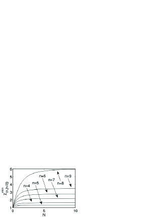
Figure 1: Minimum of the normalized potential of multipartite entanglement $\chi^{\mathrm{min}}_{(n,[n/2])}$ vs number of excitations per mode $N$, for $n=4,5,6,7,8,9$. In the region $N\ll 1$ the minimum value is linear in $N$, while it reaches a plateau for $N\gg 1$. See Sec. III for details.

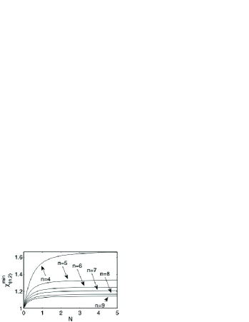
Figure 2: Minimum of the normalized potential of multipartite entanglement in the case of unbalanced bipartitions $\chi^{\mathrm{min}}_{(n,2)}$ versus $N$, for $n=4,5,6,7,8,9$. In the region $N\ll 1$ the minimum value is linear in $N$, while it reaches a plateau for $N\gg 1$. See Sec. III for details.

III Bounds on entanglement frustration in Gaussian states

In order to estimate the bounds on $\chi^{\mathrm{min}}_{(n,n_{A})}(N)$, we restrict our attention to states such that $\mathbb{K}=e^{r}\mathbb{I}_{n}$ (same squeezing for all modes), whose CM reads

$$\mathbb{V}=\frac{e^{2r}}{2}\left(\begin{array}[]{cc}\mathbb{X}\mathbb{X}^{\mathsf{T}}&-\mathbb{X}\mathbb{Y}^{\mathsf{T}}\\ -\mathbb{Y}\mathbb{X}^{\mathsf{T}}&\mathbb{Y}\mathbb{Y}^{\mathsf{T}}\end{array}\right)+\frac{e^{-2r}}{2}\left(\begin{array}[]{cc}\mathbb{Y}\mathbb{Y}^{\mathsf{T}}&\mathbb{Y}\mathbb{X}^{\mathsf{T}}\\ \mathbb{X}\mathbb{Y}^{\mathsf{T}}&\mathbb{X}\mathbb{X}^{\mathsf{T}}\end{array}\right)\,,$$ (12)

or, equivalently,

$$\mathbb{V}= \frac{\cosh{(2r)}}{2}\mathbb{I}_{2n}$$

$$+\frac{\sinh{(2r)}}{2}\left(\begin{array}[]{cc}\mathbb{X}\mathbb{X}^{\mathsf{T}}-\mathbb{Y}\mathbb{Y}^{\mathsf{T}}&-\mathbb{X}\mathbb{Y}^{\mathsf{T}}-\mathbb{Y}\mathbb{X}^{\mathsf{T}}\\ -\mathbb{Y}\mathbb{X}^{\mathsf{T}}-\mathbb{X}\mathbb{Y}^{\mathsf{T}}&\mathbb{Y}\mathbb{Y}^{\mathsf{T}}-\mathbb{X}\mathbb{X}^{\mathsf{T}}\end{array}\right)\,.$$ (15)

The energy constraints read

$$\cosh{(2r)}\leq 2N+1\,.$$ (16)

In the following we denote respectively $\tilde{\chi}_{(n,n_{A})}$ and $\tilde{\chi}^{\mathrm{min}}_{(n,n_{A})}$ the normalized potential of multipartite entanglement and its minimum evaluated for this family of states.

Table 1: Numerical estimates of the slopes $\alpha_{(n,n_{A})}$ in Eq. (24), $\tilde{\alpha}_{(n,n_{A})}$ in Eq. (23), of the minimum of the normalized potential of multipartite entanglement for $N=10$, $\chi_{(n,[n/2])}^{\mathrm{min}}(N=10)$ [which approximates $\lim_{N\to\infty}\chi_{(n,[n/2])}^{\mathrm{min}}(N)$], and of the upper bound $\beta_{(n,n_{A})}$ in Eq. (27). The results are obtained for the case of balanced bipartitions, $n_{A}=[n/2]$.

$n$	$\alpha_{(n,[n/2])}$	$\tilde{\alpha}_{(n,[n/2])}$	$\chi_{(n,[n/2])}^{\mathrm{min}}(N=10)$	$\beta_{(n,[n/2])}$
4	1.33	1.333333	1.663650	1.666667
5	1.00	1.000000	1.332326	1.333333
6	2.40	2.400000	2.780918	2.795085
7	2.00	2.000000	2.203228	2.213586
8	3.43	3.428571	5.980689	6.074700
9	3.00	3.000000	3.470522	3.491497

III.1 The linear regime, $N\ll 1$

From Eq. (15) we get

$$\tilde{\chi}_{(n,n_{A})} =$$

$$(2N+1)^{n_{A}}\mathbb{E}\left[\det\left(\cosh{(2r)}\mathbb{I}_{n_{A}}+\sinh{(2r)}\mathbb{Z}_{A}\right)^{-1/2}\right]\,,$$

where we defined

$$\mathbb{Z}:=\left(\begin{array}[]{cc}\mathbb{X}\mathbb{X}^{\mathsf{T}}-\mathbb{Y}\mathbb{Y}^{\mathsf{T}}&-\mathbb{X}\mathbb{Y}^{\mathsf{T}}-\mathbb{Y}\mathbb{X}^{\mathsf{T}}\\ -\mathbb{Y}\mathbb{X}^{\mathsf{T}}-\mathbb{X}\mathbb{Y}^{\mathsf{T}}&\mathbb{Y}\mathbb{Y}^{\mathsf{T}}-\mathbb{X}\mathbb{X}^{\mathsf{T}}\end{array}\right)\,,$$ (19)

and $\mathbb{Z}_{A}$ denotes the sub-matrix corresponding to the subset of modes $A$. Then,

$$\tilde{\chi}_{(n,n_{A})} =\left(\frac{2N+1}{\cosh{(2r)}}\right)^{n_{A}}\mathbb{E}\left[\det\left(\mathbb{I}_{n_{A}}+\tanh{(2r)}\mathbb{Z}_{A}\right)^{-1/2}\right]$$

$$\geq\mathbb{E}\left[\det\left(\mathbb{I}_{n_{A}}+\tanh{(2r)}\mathbb{Z}_{A}\right)^{-1/2}\right]\,,$$ (20)

where the inequality follows from the energy constraint, and it is saturated when $\cosh{2r}=2N+1$.

In the limit $N\ll 1$, we use the second-order expansion of the determinant,

$$\det(\mathbb{I}+\epsilon\mathbb{M})=1+\epsilon\mathrm{tr}(\mathbb{M})+\frac{\epsilon^{2}}{2}\frac{\mathrm{tr}(\mathbb{M})^{2}-\mathrm{tr}(\mathbb{M}^{2})}{2}+O(\epsilon^{3})\,.$$ (21)

By setting $\cosh{2r}=2N+1$, and noticing that $\mathrm{tr}(\mathbb{Z}_{A})=0$, we get

$$\mathbb{E}\left[\det\left(\mathbb{I}_{n_{A}}+\tanh{(2r)}\mathbb{Z}_{A}\right)^{-1/2}\right]=$$

$$1+N\mathbb{E}\left[\mathrm{tr}(\mathbb{Z}_{A}^{2})\right]+O(N^{3/2})\,.$$

Finally we obtain the upper bound:

$$\chi^{\mathrm{min}}_{(n,n_{A})}(N)\leqslant\tilde{\chi}^{\mathrm{min}}_{(n,n_{A})}(N)\leqslant 1+N\min\left\{\mathbb{E}\left[\mathrm{tr}(\mathbb{Z}_{A}^{2})\right]\right\}\,.$$ (22)

It is worth noticing that the evaluation of the upper bound still requires a constrained minimization, which is now independent of $N$. In conclusion, in the region $N\ll 1$, the minimum $\chi^{\mathrm{min}}_{(n,n_{A})}(N)$ is bounded from above by a linear function of $N$. The value of the slope

$$\tilde{\alpha}_{(n,n_{A})}:=\min\left\{\mathbb{E}\left[\mathrm{tr}(\mathbb{Z}_{A}^{2})\right]\right\}$$ (23)

has been evaluated numerically, for several values of $n$, and is presented in Table 1. A comparison with the numerical estimation of

$$\alpha_{(n,n_{A})}:=\lim_{N\to 0}\frac{\partial\chi^{\mathrm{min}}_{(n,n_{A})}(N)}{\partial N}\,,$$ (24)

also reported in Table 1, leads to conclude that the bound is tight.

III.2 Saturation, $N\gg 1$

Let us rewrite Eq. (12) as

$$\mathbb{V}=\frac{e^{2r}}{2}\left(\mathbb{W}+e^{-4r}\mathbb{W}^{\prime}\right)\,,$$

where

$$\mathbb{W}:=\left(\begin{array}[]{cc}\mathbb{X}\mathbb{X}^{\mathsf{T}}&-\mathbb{X}\mathbb{Y}^{\mathsf{T}}\\ -\mathbb{Y}\mathbb{X}^{\mathsf{T}}&\mathbb{Y}\mathbb{Y}^{\mathsf{T}}\end{array}\right)\,,\quad\mathbb{W}^{\prime}:=\left(\begin{array}[]{cc}\mathbb{Y}\mathbb{Y}^{\mathsf{T}}&\mathbb{Y}\mathbb{X}^{\mathsf{T}}\\ \mathbb{X}\mathbb{Y}^{\mathsf{T}}&\mathbb{X}\mathbb{X}^{\mathsf{T}}\end{array}\right)\,.$$

We thus obtain

$$\tilde{\chi}_{(n,n_{A})} =\frac{(N+1/2)^{|A|}}{(e^{2r}/2)^{|A|}}\mathbb{E}\left[\det\left(\mathbb{W}_{A}+e^{-4r}\mathbb{W}^{\prime}_{A}\right)^{-1/2}\right]$$

$$\geqslant\frac{(N+1/2)^{|A|}}{\left(2N+1-\frac{1}{2}e^{-2r}\right)^{|A|}}\mathbb{E}\left[\det\left(\mathbb{W}_{A}+e^{-4r}\mathbb{W}^{\prime}_{A}\right)^{-1/2}\right]\,,$$ (25)

where $\mathbb{W}_{A}$, $\mathbb{W}^{\prime}_{A}$ are respectively sub-matrices of $\mathbb{W}$, $\mathbb{W}^{\prime}$. Notice that inequality (25) is saturated if $\cosh{2r}=2N+1$.

In the limit $N\gg 1$ (i.e., $e^{-r}\ll 1$), we get

$$\tilde{\chi}_{(n,n_{A})}\geqslant 2^{-n_{A}}\mathbb{E}\left[\det(\mathbb{W}_{A})^{-1/2}\right]+O(e^{-2r})\,.$$ (26)

Then, by setting $\cosh{2r}=2N+1$, we obtain the upper bound

$$\chi^{\mathrm{min}}_{(n,n_{A})}(N) \leqslant\tilde{\chi}^{\mathrm{min}}_{(n,n_{A})}$$

$$\leqslant 2^{-n_{A}}\min\left\{\mathbb{E}\left[\det(\mathbb{W}_{A})^{-1/2}\right]\right\}$$

$$=:\beta_{(n,n_{A})}\,.$$ (27)

Notice that, also in this case, the evaluation of the right-hand side of this inequality requires a constrained minimization, now independent of the energy parameter $N$. These inequalities imply that the minimum $\chi^{\mathrm{min}}_{(n,n_{A})}(N)$ is bounded from above in the $N\to\infty$ limit. The upper bound in Eq. (27) can be evaluated numerically. Table 1 shows a comparison between the values of $\chi^{\mathrm{min}}_{(n,n_{A})}(N)$, calculated for $N=10$ (where the saturation regime has been reached of all values of $n$ considered), and the numerically estimates of $\beta_{(n,n_{A})}$. Numerical evidence suggests that the upper bound is approached in the $N\to\infty$ limit. Comparison with Eq. (7) yields then a concrete estimate for the amount of frustration in the system.

IV Conclusions

We have presented some results on entanglement frustration in multimode Gaussian states, quantified by the minimum value of the normalized potential of multipartite entanglement. Entanglement frustration arises from the impossibility for a multimode Gaussian state of being maximally bipartite-entangled across all possible bipartitions of the system. It has been proven in noi that entanglement frustration appears in multimode Gaussian states if $n_{A}\geqslant 2$, while for qubits — for the case of balanced bipartion ($n_{A}=[n/2]$) — it appears for $n=4$, $n\geqslant 8$ (the case $n=7$ is still under debate MMES1 ; others ).

The results obtained in this note extend the numerical analysis presented in noi , and put it on a more solid basis, due to the semi-analytical calculation of the upper bounds in the low and high energy regimes. Our numerical analysis suggests that these bounds are tight. In particular, the calculation of a finite upper bound in the high energy regime demonstrates that entanglement frustration remains finite in the $N\to\infty$ limit.

The results of the numerical analysis show a certain regularity in the estimates of the parameter $\alpha_{(n,n_{A})}$. The numerical estimates reported in Table 1 suggest to conjecture the following relations:

$$\alpha_{(2n_{A}+1,n_{A})} =n_{A}-1\,,$$ (28)

$$\alpha_{(2n_{A},n_{A})} =\frac{2n_{A}}{2n_{A}-1}\,\alpha_{(2n_{A}+1,n_{A})}.$$ (29)

We remark that the upper bounds are obtained by an optimization over the matrices $\mathbb{R}$ in Eq. (2), which have the property of being both symplectic and orthogonal, and hence define a representation of the unitary group $U(n)$ (see, e.g., ALN ). These observations suggest that the employment of group-theoretical methods could lead to deeper insight into the phenomenon of entanglement frustration in multimode Gaussian states.

References

• (1) I. Bengtsson and K. Zyczkowski, Geometry of Quantum States: An Introduction to Quantum Entanglement (Cambridge University Press, Cambridge, 2006).
• (2) V. I. Man’ko, G. Marmo, E. C. G. Sudarshan, F. Zaccaria, Rep. Math. Phys. 55 (2005), 405-422.
• (3) J. Grabowski, M. Kuoe, G. Marmo, J. Phys. A 38 (2005), 10217-10244.
• (4) J. F. Carinena, J. Clemente-Gallardo, G.Marmo, Theor.Math. Phys. 152 (2007) 894-903.
• (5) R. Horodecki, P. Horodecki, M. Horodecki and K. Horodecki, Rev. Mod. Phys. 81 (2009), 865-942.
• (6) P. Facchi, G. Florio, U. Marzolino, G. Parisi and S. Pascazio, New. J. Phys. 12 (2010), 025015.
• (7) A. Ferraro, S. Olivares and M. G. A. Paris, Gaussian states in continuous variable quantum information (Bibliopolis, Napoli, 2005).
• (8) P. Facchi, G. Florio, G. Parisi and S. Pascazio, Phys. Rev. A 77 (2008), 060304(R); P. Facchi, G. Florio, U. Marzolino, G. Parisi and S. Pascazio, J. Phys. A 42 (2009), 055304.
• (9) P. Facchi, G. Florio, C. Lupo, S. Mancini and S. Pascazio, Phys. Rev. A 80 (2009), 062311.
• (10) J. Zhang, G. Adesso, C. Xie and K. Peng, Phys. Rev. Lett. 103 (2009), 070501.
• (11) A. J. Scott, Phys. Rev. A 69 (2004), 052330; A. Higuchi and A. Sudbery, Phys. Lett. A 273, (2000) 213–217; I. D. K. Brown, S. Stepney, A. Sudbery and S. L. Braunstein, J. Phys. A 38 (2005), 1119; S. Brierley and A. Higuchi, ibid. 40 (2007), 8455.
• (12) P. Aniello, C. Lupo and M. Napolitano, Open Sys. & Inf. Dynamics 13 (2006), 415–426.