Spectral properties of the Wilson Dirac operator
in the $\epsilon$-regime

Abstract

We investigate the spectral properties of the Wilson Dirac operator in quenched QCD in the microscopic regime. We distinguish the topological sectors using the index as determined by the Wilson flow method. Consequently, the distributions of the low-lying eigenvalues of the Wilson Dirac operator can be compared in each of the topological sectors to predictions from random matrix theory applied to the $\epsilon$-regime of chiral perturbation theory. We find rather good agreement for volumes as small as $(1.5\,\text{fm})^{4}$ and lattice spacings as coarse as $0.1\,\text{fm}$, and demonstrate that it is indeed possible to extract low-energy constants for Wilson fermions from the spectral properties of the Wilson Dirac operator.

1 Introduction

The spontaneous breaking of chiral symmetry in Quantum Chromodynamics (QCD) is an important non-perturbative feature that determines the low-energy behaviour of the theory in a crucial way. In chiral perturbation theory, an effective description of QCD at low energies, the effect of spontaneous chiral symmetry breaking is encoded in the quark condensate $\Sigma$ and the Goldstone boson fields as the relevant degrees of freedom Weinberg:1968de ; Gasser:1983yg ; Gasser:1984gg . The effective theory then describes their dynamics while being strongly constrained by the requirements of chiral symmetry. In a specific regime of the theory, the so-called $\epsilon$-regime Gasser:1987ah ; Gasser:1987zq ; Hasenfratz:1989pk ; Hansen:1990un where the mass $m_{\pi}$ of the Goldstone pion is small compared to the linear extent $L$ of the space-time volume $V=L^{4}$, i.e. $m_{\pi}L\ll 1$, the finite volume partition function is dominated by the zero-momentum mode of the pion field. In this situation, the topology of the gauge fields becomes important and as a consequence the partition function naturally separates into sectors of fixed topology Leutwyler:1992yt .

Intriguingly, in the $\epsilon$-regime there exists another effective description of QCD which is based on random matrices Shuryak:1992pi ; Verbaarschot:1993pm ; Verbaarschot:1994qf . In Random Matrix Theory (RMT) one models the fluctuations and correlations of the energy levels of the Hamilton operator of a physical system by considering the eigenvalues of matrices with random entries, but obeying the same global symmetries. For describing the Euclidean QCD partition function, for example, one may construct a chiral random matrix model for the massless QCD Dirac operator. It turns out that in the microscopic regime this leads to the proper accumulation of eigenvalues at the origin, a characteristic feature of spontaneous chiral symmetry breaking. By now, one has a complete understanding of how and why chiral RMT represents an exact limit of the light quark partition function of QCD in the $\epsilon$-regime and a precise mapping between QCD, standard chiral perturbation theory and chiral RMT is established (see e.g. Verbaarschot:2000dy ; Damgaard:2011gc for a review and further references). As a consequence, RMT provides an interesting alternative approach for studying the universal properties of low-energy QCD.

What is common to both effective theories is the fact that their intrinsic parameters, the effective low-energy constants, need to be determined externally, either from phenomenology, or directly from QCD using calculations from first principles, e.g. lattice QCD. In the past, there have been several efforts to extract physical parameters from numerical simulations in the $\epsilon$-regime, but all of them have been restricted to the use of lattice Dirac operators which obey an exact chiral symmetry Bietenholz:2003mi ; Giusti:2003gf ; DeGrand:2006uy . Recently it has become evident, however, that simulations in the $\epsilon$-regime need not exclusively be reserved to these actions, but can also be done using standard Wilson fermions for which the chiral symmetry is broken by the discretisation. It has been understood in the context of Wilson chiral perturbation theory (WChiPT) how to include the effects of the Wilson lattice discretisation in the standard regime of the theory Sharpe:1998xm ; Rupak:2002sm ; Bar:2003mh and this has also been achieved in the $\epsilon$-regime Bar:2008th ; Shindler:2009ri . Remarkably, also chiral RMT can be extended to include the effects of the Wilson lattice discretisation, leading to Wilson chiral Random Matrix Theory (WRMT) Damgaard:2010cz ; Akemann:2010em .

Subsequently, a series of interesting statements have been made about the spectral density of the Wilson Dirac operator using WChiPT and/or WRMT for both $N_{f}=0$ (quenched) and $N_{f}=1$ QCD Damgaard:2010cz ; Akemann:2010em ; Kieburg:2011uf ; Necco:2011vx ; Necco:2011jz ; Akemann:2010zp ; Splittorff:2011bj . One motivation is that a good description of the Wilson Dirac operator spectrum is most important for lattice simulations towards the chiral limit at fixed lattice spacing. In order to perform such simulations, a thorough understanding of the quark mass, volume and lattice spacing dependence of the spectrum is crucial for avoiding potential numerical instabilities. In that respect, the quenched approximation which we are studying in this paper can still be useful for $N_{f}>0$ simulations of QCD where $m\Sigma V\gg 1$, because in that case the spectrum of the massless Dirac operator behaves essentially as in quenched QCD.

Since topology plays a crucial role in the $\epsilon$-regime it is important to have good control over the topological properties of the system. A natural definition for the topological charge of the gauge fields is provided by the Atiyah-Singer index theorem which can be carried over to the lattice for chirally symmetric lattice Dirac operators Hasenfratz:1998ri . One problem with simulating Wilson fermions in this extreme regime, though, is related to the fact that the chiral index is not well defined for the Wilson Dirac operator.

However, there exists an exact relation between the number of real modes of the Wilson Dirac operator and the index as defined from the overlap operator Narayanan:1994gw ; Neuberger:1997fp using the Wilson Dirac operator as its kernel. One way to define a topological index for the Wilson Dirac operator is then provided by the eigenvalue flow of the hermitian Wilson Dirac operator, the so-called Wilson flow method Itoh:1987iy ; Narayanan:1994gw ; Edwards:1998sh ; Edwards:1998gk ; Edwards:1999ra . The definition becomes unambiguous in the continuum limit and may hence serve as a natural definition of the index. It is an astonishing result of the WRMT descriptions Damgaard:2010cz ; Akemann:2010em ; Kieburg:2011uf that they can actually make definite statements about the hermitian eigenvalue flow and therefore make a natural connection to the various topological charge sectors of QCD.

In this paper we investigate the spectral properties of the Wilson Dirac operator in quenched QCD in the $\epsilon$-regime corresponding to the microscopic regime of WRMT by means of numerical simulations. We calculate the low-lying spectrum of the hermitian Wilson Dirac operator and compare the distributions of the single eigenvalues to the ones from WRMT. Once the matching between the QCD data and WRMT is accomplished, we can check the predictive power of WRMT by scaling and comparing the results at different masses and volumes. For distinguishing the topological charge sectors we determine the Wilson flow on each gauge field configuration. As a by-product, the Wilson flow also yields the distribution of the real modes of the Wilson Dirac operator and this can again be compared to the chirality distributions as described by WRMT.

2 Wilson random matrix theory

We start by briefly recalling the WRMT that is expected to describe the spectrum of the Wilson Dirac operator. The Symanzik expansion has three operators – $W_{6}$, $W_{7}$ and $W_{8}$ – that provide the leading order corrections for WChiPT. Arguments from a large-$N_{c}$ expansion indicate that the terms proportional to $W_{6}$ and $W_{7}$ are suppressed Kaiser:2000gs and these terms are often set to zero in a first approximation.

We consider matrices of the form

$$\tilde{D}^{\nu}_{\text{W}}=\left(\begin{array}[]{cc}\tilde{a}_{8}A&iW\\ iW^{\dagger}&\tilde{a}_{8}B\end{array}\right)\,,$$ (1)

where $A=A^{\dagger}$ and $B=B^{\dagger}$ are $(n+\nu)\times(n+\nu)$ and $n\times n$ square matrices, respectively, while $W$ is an arbitrary complex $(n+\nu)\times n$ rectangular matrix Hehl:1998pt ; Akemann:2010em . We use tildes to distinguish the quantities from the analogous ones in the quantum field theory setup. The block structure of $\tilde{D}^{\nu}_{\text{W}}$ can be interpreted as a chiral decomposition with additional terms $\propto\tilde{a}_{8}$ mixing the chiral sectors and thereby incorporating the effects of the operator $W_{8}$. Furthermore, the structure in eq.(1) guarantees that there are at least $|\nu|$ real eigenvalues. We are interested in the eigenvalues of the hermitian matrix

$$\tilde{D}_{5}^{\nu}(\tilde{m})=\tilde{\gamma}_{5}(\tilde{D}_{\text{W}}^{\nu}+\tilde{m})$$ (2)

where $\tilde{\gamma}_{5}=\text{diag}(1,\ldots,1,-1,\ldots,-1)$ with $(n+\nu)$ entries of 1 and $n$ entries of $-1$ along the diagonal.

The matrix elements of $\tilde{D}^{\nu}_{\text{W}}$ are randomly distributed according to the Gaussian weight

$$P(A,B,W)=e^{-\frac{N}{4}\text{Tr}[A^{2}+B^{2}]-\frac{N}{2}\text{Tr}[WW^{\dagger}]}\,$$ (3)

with $N=2n+\nu$. The partition function $\tilde{Z}_{N_{f}}^{\nu}$ for the WRMT is then given by integrating the matrices $A,B,W$ over the complex Haar measure with the weight $P(A,B,W)$, i.e.,

$${\tilde{Z}_{N_{f}}^{\nu}}(\tilde{m},\tilde{z};\tilde{a}_{8})=\int{\cal D}A\,{\cal D}B\,{\cal D}W\text{det}(\tilde{D}^{\nu}_{\text{W}}+\tilde{m}+\tilde{z}\tilde{\gamma}_{5})^{N_{f}}P(A,B,W)\,.$$ (4)

The additional operators introduced by the Wilson lattice discretisation can be incorporated by extending the partition function using the definition

$${\tilde{Z}_{N_{f}}^{\nu}}(\tilde{m},\tilde{z};\tilde{a}_{6},\tilde{a}_{7},\tilde{a}_{8})=\int_{-\infty}^{\infty}dy_{6}dy_{7}e^{-\frac{y_{6}^{2}}{16|\tilde{a}_{6}^{2}|}-\frac{y_{7}^{2}}{16|\tilde{a}_{7}^{2}|}}{\tilde{Z}_{N_{f}}^{\nu}}(\tilde{m}-y_{6},\tilde{z}-y_{7};\tilde{a}_{8})\,.$$ (5)

Finally, the microscopic limit of WRMT is reached in the limit $N\rightarrow\infty$ while

$$\tilde{m}N,\quad\tilde{z}N,\quad\tilde{a}_{i}N^{1/2}$$ (6)

are kept fixed. It is therefore natural to think of $N$ as corresponding to the space-time volume in the quantum field theory setup. One can show that the WRMT partition function reproduces the leading terms in the $\epsilon$-expansion of WChiPT Akemann:2010em and the corresponding low-energy constants can be identified as

$$\tilde{m}N\propto m\Sigma V,\quad\tilde{z}N\propto z\Sigma V,\quad\tilde{a}_{i}^{2}N\propto a^{2}\,W_{i}V.$$ (7)

Note that the WRMT setup described here can only reproduce WChiPT with a fixed choice for the signs of the low-energy constants. Using the conventions of Akemann:2010em , $\tilde{a}_{8}$ will map into a positive $W_{8}$, while non-zero values $\tilde{a}_{6}$ and $\tilde{a}_{7}$ imply negative values for $W_{6}$ and $W_{7}$. From the corresponding partition functions analytic expressions for the distributions of the eigenvalues of the QCD Dirac operator in the $\epsilon$-regime can be obtained both in WChiPT Akemann:2010em and in WRMT Kieburg:2011uf .

3 Lattice setup

Before discussing our results we also need to specify the setup for our lattice calculation. The massive Wilson-Dirac operator can be written as

$$D_{\text{W}}(m)=\frac{1}{2}\gamma_{\nu}(\nabla_{\nu}+\nabla_{\nu}^{*})-\frac{1}{2}\nabla_{\nu}^{*}\nabla_{\nu}+m,$$ (8)

where $\nabla_{\nu},\,\nabla_{\nu}^{*}$ denote the covariant forward and backward lattice derivatives, respectively, $\gamma_{\nu}$ are the Euclidean Dirac matrices and $m$ is the bare quark mass. The Wilson-Dirac operator is $\gamma_{5}$-hermitian,

$$D_{\text{W}}^{\dagger}=\gamma_{5}D_{\text{W}}\gamma_{5}$$ (9)

and hence

$$D_{5}=\gamma_{5}D_{\text{W}}(m)$$ (10)

is hermitian, $D_{5}^{\dagger}=D_{5}$. The dependence of the eigenvalues $\lambda_{k}^{5}(m)$ of $D_{5}(m)$ on $m$ defines the eigenvalue flow and from first order perturbation theory one can infer

$$\frac{d\lambda^{5}_{k}}{dm}=\langle k|\gamma_{5}|k\rangle\,.$$ (11)

The eigenvalues of $D_{\text{W}}$ are denoted by $\lambda_{k}^{\text{W}}$. Since the Wilson Dirac operator is non-normal, i.e. $[D_{\text{W}},D_{\text{W}}^{\dagger}]\neq 0$, one needs to distinguish the left and right eigenvectors which define a bi-orthogonal system. As a consequence the eigensystems of $D_{\text{W}}$ and $D_{5}$ are related in a non-trivial way, except for the subset of $D_{5}$-eigenvalues which are exactly zero for a given value of $m$. In that case one has

$$\gamma_{5}(D_{\text{W}}+m)\psi=0\quad\Longleftrightarrow\quad D_{\text{W}}\psi=-m\psi\,,$$ (12)

i.e., a real mode $\lambda_{k}^{\text{W}}\in{\mathbb{R}}$ of $D_{\text{W}}$ corresponds to a zero mode of $D_{5}(m=-\lambda_{k}^{\text{W}})$ and the chirality of the mode is given by the derivative of the Wilson flow, eq.(11), at $m=-\lambda_{k}^{\text{W}}$.

Here we are specifically interested in the chirality distribution of the real modes $\lambda_{k}^{\text{W}}$ of $D^{\nu}_{\text{W}}$ defined as

$$\rho_{\chi}(\lambda)=\left\langle\sum_{\lambda_{k}^{W}\in\mathbb{R}}\delta(\lambda_{k}^{W}+\lambda)\text{sign}(\langle k|\gamma_{5}|k\rangle)\right\rangle\,$$ (13)

and the distribution of the $k$-th eigenvalue $\lambda_{k}^{5}(m)$ of $D_{5}$ given by

$$\rho^{k}_{5}(\lambda,m)=\left\langle\delta(\lambda_{k}^{5}(m)-\lambda)\right\rangle\,.$$ (14)

These are the distributions which we compare to the analytic expressions obtained from WRMT. Up to now only the expression for the full distribution $\rho_{5}=\sum_{k}\rho^{k}_{5}$ is known, so the single eigenvalue distributions $\rho_{5}^{k}$ are obtained from WRMT directly by numerical simulation.

3.1 Definition of the topological charge

A crucial ingredient for the proper treatment of the configurations in the analysis is their correct assignment to the various topological sectors. As discussed in Akemann:2010em summing up the signs of the chiralities of the real modes $\lambda_{k}^{W}\in{\mathbb{R}}$ of $D_{\text{W}}$ for a given gauge field configuration yields an index of the Wilson Dirac operator,

$$\nu=\sum_{\lambda_{k}^{W}\in\mathbb{R}}\text{sign}(\langle k|\gamma_{5}|k\rangle)\,.$$ (15)

Note that the sum over the real modes is actually only a sum over the real modes of $D_{\text{W}}(m)$ in the neighbourhood of $m$, i.e. it excludes the doubler real modes. Since the real modes are in correspondence with the zero modes of $D_{5}$, this index is in agreement with the topological charge as defined through the Wilson flow method Itoh:1987iy ; Narayanan:1994gw ; Edwards:1998sh ; Edwards:1998gk ; Edwards:1999ra . In practise, the Wilson flow yields all the real modes of $D_{\text{W}}$ up to a cut-off $m_{\text{cut}}$, so the practical realisation of eq.(15) is given by

$$\nu=\sum_{\lambda_{k}^{W}<m_{\text{cut}}}\text{sign}(\langle k|\gamma_{5}|k\rangle)\,,$$ (16)

where the restriction takes into account only the real modes up to a certain cut-off $m_{\text{cut}}$. Consequently all real modes with $\lambda_{k}^{W}>m_{\text{cut}}$ are considered to correspond to doubler modes. In that sense the topological charge is not well defined at finite lattice spacing – as it should be – but becomes so in the continuum limit. This ambiguity is not a surprise and is reflected in any definition of the topological charge at finite lattice spacing. In particular, also the definition of the topological charge via the index of the overlap Dirac operator Neuberger:1997fp ,

$$D_{\text{o}}=1+\gamma_{5}\,\text{sign}[\gamma_{5}D_{\text{K}}(-m)]\,,$$ (17)

is ambiguous, since it depends on the mass shift $-m$ entering the definition of the hermitian kernel Dirac operator $\gamma_{5}D_{\text{K}}$. The correspondence between the index of the overlap operator and the charge from the eigenvalue flow is exact, so $m$ in the overlap operator corresponds to $m_{\text{cut}}$ in the definition eq.(16).

While the chirality of the real modes is $\pm 1$ in the continuum, for the non-normal Wilson Dirac operator this holds only approximately (cf. also Kerler:1999dk ; Kerler:1999iv ). The non-normality of $D_{\text{W}}$ is a consequence of its specific symmetry structure and can not be avoided, however, one can reduce it, e.g., by modifying the covariant derivatives. In our study we use covariant derivatives with various levels of HYP-smeared gauge fields, since this is a simple but efficient mean of suppressing the non-normality Durr:2005an . The effect of the smearing is manifold. Most importantly, it improves the separation of the physical zero modes from the doubler zero modes and in this way reduces the ambiguity of the charge definition, i.e. its dependence on $m_{\text{cut}}$. As a side effect, the chirality of the zero modes is improved significantly with increasing smearing level.

Obviously, any remaining ambiguity in the topological charge assignment is due to additional crossings beyond the value of $m_{\text{cut}}$ employed in the charge definition. Interestingly, WRMT can make predictions about the number of these additional crossings Kieburg:2011uf and we will investigate this in section 4.3.1.

Based on these considerations, we present in the following the results for a Wilson Dirac operator with covariant derivatives based on gauge fields with 5 HYP-smearing levels, and use eq.(16) as our definition of the topological charge with $m_{\text{cut}}$ as given in table 1.

3.2 Simulation parameters

We have simulated several lattices with various sizes and lattice spacings in $N_{f}=0$ QCD using the Wilson gauge action. The simulation parameters for these quenched ensembles are described in table 1. Within the group $A$ we have kept the lattice spacing constant in order to study potential finite volume effects. In contrast, for ensembles $A_{1}$ and $B_{1}$ the volume $V=L^{3}\times L_{t}$ is roughly kept constant in physical units.

lattice	$\beta$	$L/a$	$L_{t}/a$	$r_{0}/a$	$L[\text{fm}]$	$m_{\text{cut}}$	$\mathrm{d}|\nu|/\mathrm{d}m\big{|}_{m_{\text{cut}}}$
$A_{1}$	6.20	$24$	$24$	7.36	1.53	0.19	0.60(40)
$A_{2}$	6.20	$20$	$20$	7.36	1.28	0.30	0.14(11)
$B_{1}$	5.90	$14$	$16$	4.48	1.47	0.50	0.12(13)

Table 1: Simulation parameters for the $N_{f}=0$ ensembles together with the value of $m_{\text{cut}}$ used in the definition of the topological charge.

Table 1 also provides a numerical estimate of the derivative of the charge with respect to the cut employed in the Wilson flow. A graphical presentation of this quantity as a function of the mass is shown for each of the ensembles in figure 1.

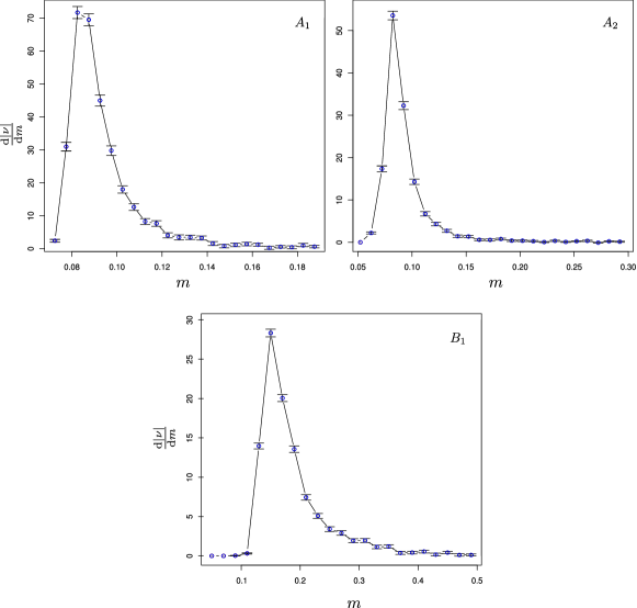
Figure 1: Derivative of the absolute charge with respect to $m_{\text{cut}}$ for the ensembles described in table 1.

The derivative in each of the ensembles shows a sharp peak in the neighbourhood of the critical mass, after which a more or less rapid decay sets in depending on the volume and the lattice spacing. In absolute terms, the derivative of the charge is practically negligible at the point where the mass cut is introduced. Using a linear extrapolation through the tail of the distributions as a rough estimate, we should expect to be misassigning up to half a percent of the configurations in ensemble $B_{1}$ and at most about one percent for the ensembles $A_{1}$ and $A_{2}$.

4 Results

4.1 Cumulative hermitian eigenvalue distributions

We start by considering the distributions $\rho_{5}(\lambda)$ of the eigenvalues of the hermitian Wilson Dirac operator $D_{5}$ and compare them with the analytic expressions. So far the expressions from WRMT and WChiPT comprise only the full distributions for the lowest lying eigenvalues. In figure 2 we show the full

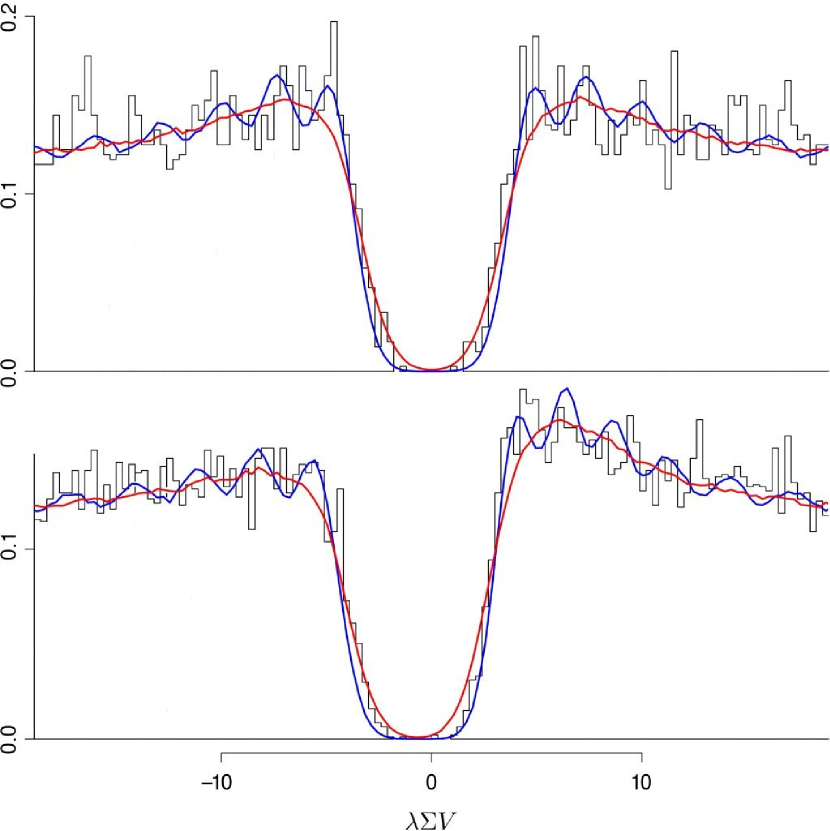
Figure 2: The density of the lowest lying eigenvalues in the topological charge sectors $\nu=0$ (top) and $\nu=1$ (bottom), for the ensembles $A_{1}$. Blue lines are fits accounting just for $W_{8}$, red lines are fits including the effects of $W_{6}$ and $W_{7}$. These lines were calculated by means of WRMT, using 250k samples.

distributions for our ensemble $A_{1}$ in the charge sectors $\nu=0$ and $\nu=1$, together with fits to both that will be discussed in more detail below. Some of the expected features of the spectrum are apparent, the most prominent being the enhanced peak on the positive side for $\nu=1$. However, it is clear – also from a comparison of the data to the relatively delicate features of the fitted lines – that it would be rather challenging to push the analysis beyond a qualitative comparison on the basis of these distributions alone. Luckily, our data obtained from the simulations contain much more information than just the full distribution, since we have access to each single low-lying eigenvalue. Indeed it turns out that the shapes of the single eigenvalue distributions are rather sensitive to the low-energy constants $W_{6},W_{7}$ and $W_{8}$. For this reason, our fits concern single eigenvalue distributions obtained from explicit WRMT simulations including the effects of $W_{8}$ and possibly $W_{6},W_{7}$. The fit parameters in WRMT are then $\tilde{m},\tilde{a}_{6},\tilde{a}_{7},\tilde{a}_{8}$ and $\Sigma V$ which sets the scale and connects the WRMT to the QCD data.

Binning the data into histograms introduces an unwelcome dependence on the bin size and hence we choose to compare cumulative distributions. In order to assess the quality of the fits we employ the Kolmogorov-Smirnov (KS) test statistics. If $S_{\text{QCD}}(x)$ and $S_{\text{WRMT}}(x)$ are the estimates of the cumulative distribution functions obtained from the QCD and the WRMT simulation, respectively, the KS statistics is given by

$$d_{\text{max}}=\operatorname*{max}_{-\infty<x<\infty}|S_{\text{QCD}}(x)-S_{\text{WRMT}}(x)|\,.$$ (18)

Since we fit several distributions at once, it is not clear how to translate $d_{\text{max}}$ into a quality of fit measure and we will restrict ourselves to reporting only the value of $d_{\text{max}}$.

Finally, the errors on the distributions we present in the following are obtained by a bootstrap procedure and for better visibility represent a 95% confidence bound, rather than a regular standard deviation.

A summary of all the fit results discussed in this paper is given in table 2 for convenient reference.

	ens.	$|\nu|$	$N_{\text{conf}}$	$m$	$N\tilde{m}$	$\tilde{a}_{6}N^{1/2}$	$\tilde{a}_{7}N^{1/2}$	$\tilde{a}_{8}N^{1/2}$	$\Sigma V$	$d_{\text{max}}$
$F_{1}$	$A_{1}$	1	1602	-0.07	5.3(2)	0.25(7)	0.25(5)	0.70(13)	308.3(5.8)	0.061
$F_{2}$	$A_{1}$	0	462	-0.07	5.5(4)	0.27(4)	0.27(2)	0.82(13)	299.6(3.4)	0.064
$F_{3}$	$A_{1}$	1	1602	-0.07	5.5(2)	0.23(9)	0.27(2)	0.83(06)	300.4(2.2)	0.087
$F_{4}$	$A_{1}$	2	612	-0.07	5.6(3)	0.18(7)	0.27(5)	0.84(13)	301.1(8.6)	0.152
$F_{5}$	$A_{1}$	0	462	-0.07	5.4(–)	0	0	0.85(–)	295.2(–)	0.091
$F_{6}$	$A_{1}$	1	1602	-0.07	5.7(–)	0	0	0.96(–)	303.7(–)	0.155
$F_{7}$	$A_{1}$	0	462	-0.055	8.8(8)	0.22(7)	0.22(4)	0.63(19)	296.3(21.9)	0.149
$F_{8}$	$A_{1}$	1	1602	-0.055	8.2(8)	0.23(5)	0.23(9)	0.51(19)	282.8(9.8)	0.129
$F_{9}$	$A_{2}$	0	601	-0.07	4.0(1.6)	0.20(4)	0.18(4)	0.76(32)	156.9(21.5)	0.196
$F_{10}$	$A_{2}$	1	1558	-0.07	4.9(2.5)	0.32(5)	0.29(5)	0.77(26)	170.8(21.4)	0.346
$F_{11}$	$B_{1}$	0	624	-0.1	7.6(7)	0.29(20)	0.29(13)	0.82(13)	150.9(5.7)	0.091
$F_{12}$	$B_{1}$	1	1241	-0.1	6.8(7)	0.29(14)	0.27(14)	0.77(32)	141.4(4.9)	0.260

Table 2: Fit results for the fits of WRMT to the QCD ensembles $A_{1},A_{2}$ and $B_{1}$ in the various topological sectors $|\nu|$. $N_{\text{conf}}$ denotes the number of configurations used in the fits. The bare mass $m$ of the Dirac operator and $\Sigma V$ are given in lattice units, while the remaining columns are the fitted dimensionless WRMT parameters. The total number of the lowest-lying eigenvalues fitted on both the positive and negative side of the spectrum is $N_{\text{ev}}=4$ for fit $F_{1}$ and $N_{\text{ev}}=8$ for all other fits.

4.1.1 Influence of $W_{6}$ and $W_{7}$

As mentioned above, large-$N_{c}$ arguments indicate that the terms proportional to $W_{6}$ and $W_{7}$ are suppressed Kaiser:2000gs . In order to assess the importance of these low-energy constants we compare fits including only $W_{8}$ (fits $F_{5}$ and $F_{6}$ in table 2) to ones which include all three low-energy parameters $W_{6},W_{7}$ and $W_{8}$ (fits $F_{2}$ and $F_{3}$). The resulting distributions obtained in ensemble $A_{1}$ in charge sector $\nu=0$ at $m=-0.07$ are displayed in figure 3 and a visual examination makes it clear that the fits including $W_{6},W_{7}$ are superior in describing the shapes of the single eigenvalue distributions. This is corroborated by the values of $d_{\text{max}}$ in table 2 which grow by about 30-50% when $W_{6},W_{7}$ are excluded. So while $W_{8}$ appears to account for large parts of the deviation from the chiral setup, we do find $W_{6}$ and $W_{7}$ to be important as well and henceforth include them in all further fits.

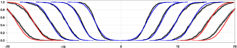
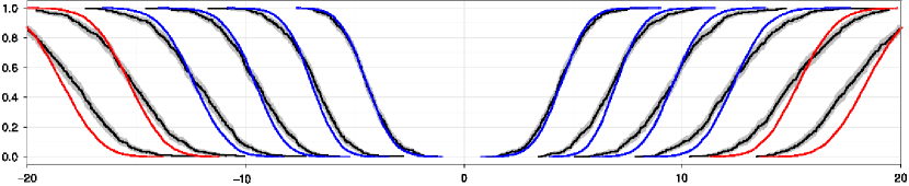
$\lambda\Sigma V$

Figure 3: Cumulative eigenvalue distributions for ensemble $A_{1}$ in charge sector $\nu=0$ compared to WRMT fits including contributions from low-energy constants $W_{6},W_{7},W_{8}$ (fit $F_{2}$, upper plot) and only $W_{8}$ (fit $F_{5}$, lower plot). Blue lines denote fitted distributions from WRMT, red lines are the predictions following from the fit.

Fits including and excluding the effects of $W_{6}$ and $W_{7}$ have also been added to figure 2. Here one can clearly observe the influence of the additional operators, that work to largely wash out the characteristic but subtle undulating pattern observed on top of the spectrum as predicted by the WChiPT expressions Akemann:2010em . Our observation that fitting these added parameters tends to produce non-vanishing values implies that one should not necessarily expect to observe such a pattern in practise. This once again underlines the importance of examining the distributions of the separate eigenvalues rather than the overall distribution, as the apparent impact of these operators would imply few distinct features of the spectrum remain to constrain fits by.

4.1.2 Sensitivity to topology and predictive power

Next we investigate the sensitivity of the WRMT fits to the various topological sectors and the predictive power of the fits as a first non-trivial test. A possible way to proceed is to fit the distributions of a selected set of eigenvalues in a given topological sector to the distributions obtained from WRMT and check the consistency for the other eigenvalues and in the other topological sectors.

In figure 4

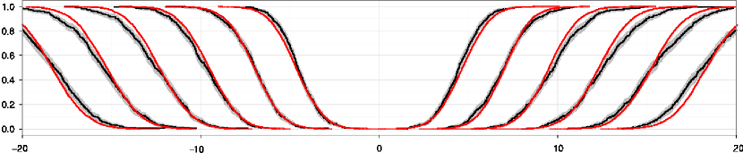
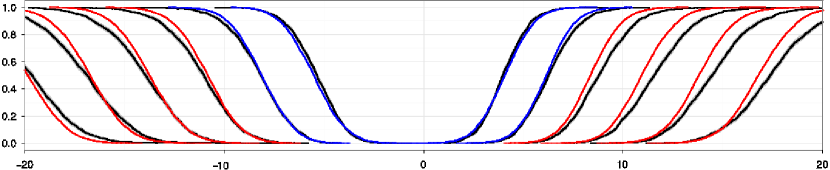
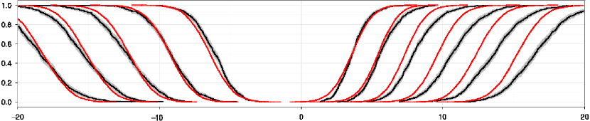
$\lambda\Sigma V$

Figure 4: Cumulative eigenvalue distributions for ensemble $A_{1}$ in charge sectors $\nu=0,1$ and 2 from top to bottom. The QCD data is displayed in black. Blue lines denote the fitted distributions from WRMT (fit $F_{1}$ in table 2), while red lines are the predictions following from the fit.

we show the results of such an exercise for the spectrum of $D_{5}$ at a bare mass $m=-0.07$. We choose to fit the distributions of the lowest two positive and negative eigenvalues in the charge sector $\nu=1$, since this is where we have the largest statistics. As before, the fitted cumulative WRMT distributions are displayed as the blue lines, while the red lines are the predictions for the remaining eigenvalue distributions following from the fit. The results for the fit parameters and the value of $d_{\text{max}}$ can be found in table 2 in the row labelled by $F_{1}$.

A number of observations can be made at this point:

(1) The four eigenvalue distributions in the charge sector $\nu=1$ can be described very well by WRMT, both in terms of the position and the shape, as reflected by the low value of $d_{\text{max}}$ reported in table 2.
(2) The distributions in the charge $\nu=0$ sector are all predictions. Again, the agreement is very good up to about $|\lambda|\Sigma V\simeq 12$ where deviations in the tail of the distributions away from 0 start to show up. One may assign this to the onset of the bulk which could be related to the Thouless energy where the RMT description is expected to break down.
(3) For the predicted distributions in the charge $\nu=1$ sector we find that WRMT tends to underestimate the tails of the eigenvalue distributions away from 0.
(4) The same effect is visible in the other predicted eigenvalue distributions in charge sector $\nu=2$, but in addition we now also find a mismatch in the position of the distributions.
(5) It seems that both these mismatches are more severe on that side of the spectrum where the would-be real modes are accumulating. One may conclude from this that lattice artefacts seem to be pushed from the would-be real modes to the nearby modes in the spectrum, and that this effect is enhanced for increasing topology.

4.1.3 Scaling of the distributions

An important prediction of the WRMT is the universal scaling of the distributions with the volume, as implied by equation 7, and with the mass.

We first investigate the scaling of the distributions with the volume. For this purpose we compare our best fits $F_{2-3}$ on ensemble $A_{1}$ with a volume $V_{1}=(1.52\text{fm})^{4}$ in the charge sectors $\nu=0,1$ to the corresponding fits $F_{9-10}$ on ensemble $A_{2}$ with volume $V_{2}=(1.28\text{fm})^{4}$. Both data sets are obtained at $m=-0.07$. The fits are displayed for visual inspection in figure 5 for $A_{1}$ and figure 6 for $A_{2}$. We note that the quality of the fits on the smaller volume is clearly deteriorating, with $d_{\text{max}}$-values increasing by a factor 3 in charge sector $\nu=0$ and 4 in sector $\nu=1$. We assign this to the fact that the volume $V_{2}=(1.28\text{fm})^{4}$ is clearly too small for the system to be in the $\epsilon$-regime. Nevertheless, with the results in table 2 we may quantitatively check the scaling of the parameters. We expect

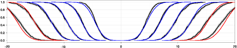
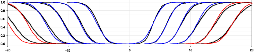
$\lambda\Sigma V$

Figure 5: Cumulative eigenvalue distributions for ensemble $A_{1}$ with volume $V_{1}=(1.52\text{fm})^{4}$ together with the best fits to WRMT. Charge sector $\nu=0$ (top, fit $F_{2}$) and $\nu=1$ (bottom, fit $F_{3}$).

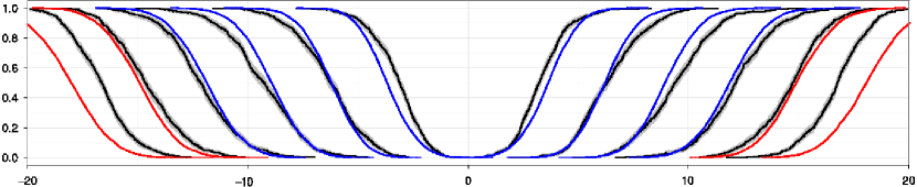
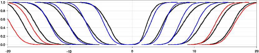
$\lambda\Sigma V$

Figure 6: Cumulative eigenvalue distributions for ensemble $A_{2}$ with $V_{2}=(1.28\text{fm})^{4}$ together with the best fits to WRMT. Charge sector $\nu=0$ (top, fit $F_{9}$) and $\nu=1$ (bottom, fit $F_{10}$).

$\tilde{a}_{6},\tilde{a}_{7}$ and $\tilde{a}_{8}$ to scale like $(V_{1}/V_{2})^{1/2}=1.41$ and $\Sigma V$ like $V_{1}/V_{2}=2.0$. Except for $\tilde{a}_{8}$ this is what we roughly observe at least in the charge sector $\nu=0$ where the small volume is indeed better described by WRMT.

Next we investigate the scaling of the distributions with the mass. For this purpose we plot in figure 7 the distributions obtained on $A_{1}$ in the charge sectors $\nu=0,1$ at a different value of the bare mass of $m=-0.055$. These fits should again be compared with those in figure 5.

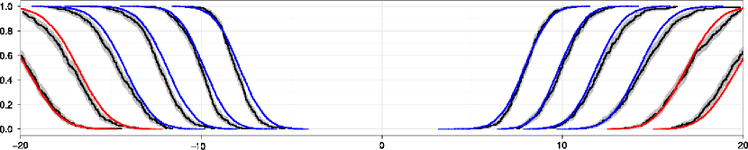
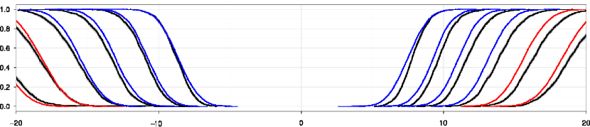
$\lambda\Sigma V$

Figure 7: Cumulative eigenvalue distributions for ensemble $A_{1}$ at bare mass $m=-0.055$ in charge sectors $\nu=0$ (top, fit $F_{7}$) and $\nu=1$ (bottom, fit $F_{8}$).

From a comparison of the fit parameter $\tilde{m}$, we can infer a value of the critical mass $m_{\text{crit}}\sim-0.09$. As we will see in section 4.3 this matches rather well with what we find from the distributions of the real modes. On the other hand, we observe a rather poor quality of the fits $F_{7}$ and $F_{8}$ as compared to $F_{2}$ and $F_{3}$. Of course, the increase in mass will push all the eigenvalues in the spectrum towards the bulk making it more difficult for the WRMT to describe them properly. Indeed, this is also reflected in the enhanced errors on all the fit parameters impeding a more quantitative comparison of the two spectra at different masses.

4.2 Eigenvalue averages

With respect to the full eigenvalue distributions discussed in the previous section, averages of single eigenvalues represent a strong reduction of the amount of information available for a comparison. Nevertheless, since the averages can be determined to high statistical precision, a comparison between the QCD data and the WRMT description at this level may indicate systematic deviations more clearly. Figure 8 summarises the results of our fits to the two main ensembles $A_{1}$ and $B_{1}$ in terms of these averages. The plots show the averages for each separate eigenvalue, both as measured on the lattice and as produced by the fitted WRMT. In each topological charge sector, values on the left denote the negative eigenvalues, while the values on the right give the positive ones. For the charge sector $\nu=0$ the two sides are symmetric and have been merged.

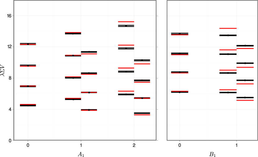
Figure 8: Comparison of the measured and fitted eigenvalue averages, for the ensembles $A_{1}$ and $B_{1}$ in the different topological charge sectors. Negative eigenvalues are plotted to the left, positive eigenvalues to the right. Black points indicate the measured data, while red lines indicate the values from WRMT based on the fits $F_{2}$, $F_{3}$, $F_{4}$, $F_{11}$ and $F_{12}$ from table 2.

We find that the WRMT appears to work very well for trivial topology, both for the coarse ensemble $B_{1}$ and the smooth one $A_{1}$, as can also be inferred from table 2. For higher charges, however, the eigenvalues with chiralities opposite to the sign of the topological charge are systematically pulled towards zero, while the ones with the same chirality sign come out higher than what WRMT tends to predict. This points to the mixing between eigenvalue sectors of different chirality being stronger, and hence lattice artefacts being larger than what WRMT is able to describe. The effect seems to be more pronounced in the higher charge sectors and at coarser lattice spacing. This is corroborated by the fact that for the ensemble $A_{1}$ the charge sector $\nu=1$ is still well described, whereas for $B_{1}$ large deviations start to appear already there.

4.3 Chirality distributions

The determination of the topological charge through the Wilson flow provides us with all the zeros of $D_{5}(-m)$ up to the cut-off $m_{\text{cut}}$ together with their associated chirality. According to the relationship in eq.(12), the locations of these zeros can be directly related to the real eigenvalues $\lambda_{k}^{\text{W}}$ of the operator $D_{\text{W}}$. The latter can also be directly obtained from WRMT, once the parameters have been determined, allowing for the comparison of the chirality distributions.

Figure 9 shows a comparison of the chirality distributions that were measured for our ensembles $A_{1}$ (in red) and $B_{1}$ (in blue). Empty bars show the number of eigenvalues with positive and negative chirality, while the filled bars give the net chirality distribution. To simplify the comparison, the measured values of $\lambda\equiv-\lambda_{k}^{\text{W}}$ were multiplied by $\Sigma V$ as determined from our fits and shifted such that the peak of the distribution is located at 0 in a rough approximation of the critical mass. The distributions for $B_{1}$ were rescaled to compensate for differences in the statistics per charge sector.

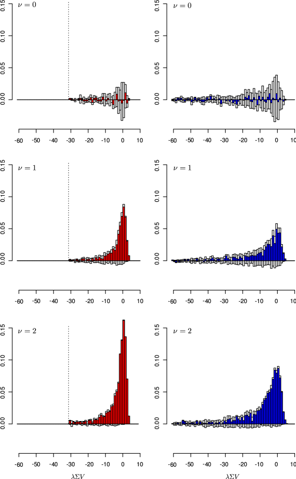
Figure 9: Chirality distributions for the three lowest charge sectors of ensembles $A_{1}$ (red) and $B_{1}$ (blue). The distributions have been shifted for convenient comparison and have been normalised to contain the same statistics per charge sector. The dotted line corresponds to the value of $m_{\text{cut}}$ employed for the calculation of the charge in ensemble $A_{1}$.

The distributions for both ensembles $A_{1}$ and $B_{1}$ are sharply peaked around $m_{c}$, but long tails remain towards more negative values of $\lambda$. It is clear that the distribution is more sharply peaked, and the tail shorter, for the ensemble $A_{1}$ with its significantly smaller lattice spacing. In addition, the number of cancellations is significantly higher for the ensemble $B_{1}$. The occurrence of conjugate pairs of real modes with opposite chirality, responsible for these cancellations, will be suppressed towards the continuum limit. This comparison therefore shows a clear decrease in discretisation artifacts.

Analytical results for the chiral density Akemann:2010em based on WChiPT tend to show a distinct structure of merged peaks, the number of which is given by the topological charge. This is in contrast to what we observe in any of our ensembles. One possible cause of this could be the influence of the $W_{6}$ and $W_{7}$ operators, as already indicated in figure 2. To investigate this further, we obtained the real eigenvalues from 100k samples of the WRMT with $\nu=2$. We used sets of parameters matching our $A_{1}$ ensemble, both including $\tilde{a}_{6}$ and $\tilde{a}_{7}$. The chirality distributions obtained from this calculation are provided in figure 10.

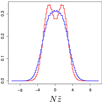
Figure 10: Chirality density as calculated by WRMT for $\nu=2$, excluding (red) and including (blue) the effect of $\tilde{a}_{6}$ and $\tilde{a}_{7}$.

The effect of the additional operators is clearly observable, as the peak is broadened and all internal structure wiped out. Given the non-vanishing values we find for the parameters $\tilde{a}_{6}$ and $\tilde{a}_{7}$ in our fits, we should not expect to see any structure in our chirality distributions.

While real eigenmodes can and do appear for the topologically trivial sector, a chirality distribution equal to zero is guaranteed because of the symmetry between positive and negative values of the topological charge. In order to facilitate a quantitative comparison between the chirality distributions of QCD and the ones from WRMT in the sectors with non-trivial topology we again consider the cumulative distributions. Figure 11 shows those

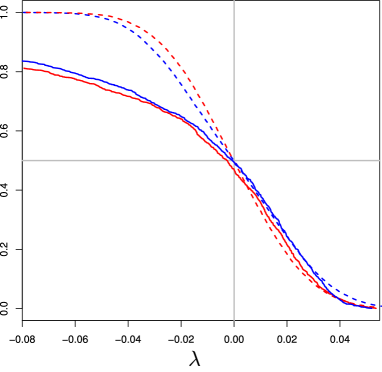
Figure 11: Cumulative distribution function for the chirality distribution of the $A_{1}$ ensemble. Red lines refer to $\nu=1$, blue lines to $\nu=2$. Solid lines are obtained from the QCD simulation, while dashed lines indicate the expectation from WRMT.

found in ensemble $A_{1}$ from configurations with $\nu=1$ (red) and 2 (blue) in solid lines, with the WRMT predictions in dashed lines. Note that in this plot, $m_{\text{cut}}$ would correspond to a value of $\lambda=-0.3$.

We find a clear distinction between the QCD and the WRMT distributions, as the QCD results are asymmetric around 0. It is interesting, however, to observe that the distributions do in fact match quite well up to the determined value of the critical mass. Beyond that point, the chirality distribution as described by WRMT drops to zero quite rapidly, while crossings keep occurring for the QCD theory. The fact that the derivative of the absolute charge with respect to the mass cut-off has become very small for larger values of the cut-off (cf. table 1) shows that this deviation cannot be attributed straightforwardly to a lack of statistics or misassigned configurations. On the other hand, the structure of the WRMT prevents any of the operators included from breaking the symmetry of the distribution around 0, so the mismatch must be due to lattice artefacts in the chirality distributions which appear not to be described by WRMT.

4.3.1 Additional modes

Apart from the chirality distribution, WRMT and WChiPT allow for inferring a relationship between the charge sector and the average number of additional crossings $N_{\mathrm{add}}$, i.e., the difference between the total number of crossings found in the Wilson flow and the absolute charge of the configuration. For small lattice spacing $a$, this relationship is given in Kieburg:2011uf as

$$N_{\mathrm{add}}\propto a^{2(\nu+1)},$$ (19)

a pure power law. The determination of $N_{\mathrm{add}}$ becomes progressively harder for larger values of the charge, as both the number of such configurations and the expectation value of $N_{\mathrm{add}}$ decrease rapidly. Nevertheless, the data for ensembles A1 and B1 displayed in figure 12 appears consistent with the predicted power-law behaviour. Moreover, the ratio of the coefficients of the linear terms should be given by the ratio of the lattice spacings. Performing linear fits to the initial three (for $A_{1}$) and four (for $B_{1}$) points, we obtain the coefficients -0.785 and -0.471, respectively. The ratio then comes out as 1.67, to be compared to 1.64 from the ratio of lattice spacings as given by $r_{0}/a$. This excellent agreement may be somewhat accidental here, given the limited number of reliable points and the clear sensitivity to the fit range. Nevertheless, we conclude that there are strong indications that the power law for $N_{\mathrm{add}}$ derived in Kieburg:2011uf holds for our data, in spite of the limited agreement with the prediction for the chirality distribution and the somewhat coarse lattice spacing in $B_{1}$.

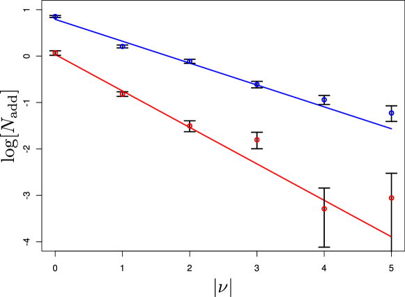
Figure 12: The logarithm of the average number of additional crossings $N_{\mathrm{add}}$ versus the absolute charge $|\nu|$. Shown are values for ensemble $A_{1}$ (red) and $B_{1}$ (blue).

5 Conclusions

We have investigated the spectral properties of the Wilson Dirac operator on the lattice for $N_{f}=0$ quenched QCD in the $\epsilon$-regime by numerical simulations. The resulting eigenvalue distributions $\rho_{5}(\lambda)$ of the hermitian Wilson Dirac operator $D_{5}$ and the chirality distributions $\rho_{\chi}(\lambda)$ of the real modes of the Dirac operator $D_{\text{W}}$ can be compared to expressions resulting from Wilson chiral perturbation theory (WChiPT) in the $\epsilon$-regime, or equivalently by Wilson random matrix theory (WRMT) in the microscopic limit. In order to do so, it is important to have good control over the different topological sectors of QCD and we have taken care of this by employing the topological index based on the eigenvalue flow of $D_{5}$ as the definition of the topological charge. Towards the continuum limit this definition becomes equivalent to the index of the overlap operator.

Concerning the eigenvalue distributions $\rho_{5}^{k}(\lambda)$ of the $k$-th eigenvalue, we find that they can be described rather well by the corresponding distributions as given by the WRMT. It turns out that by fitting these distributions, it is indeed possible to extract the leading low energy constants $W_{6},W_{7}$ and $W_{8}$ for Wilson fermions from the eigenvalue spectra of the Wilson Dirac operator in the $\epsilon$-regime, on volumes as small as $V\sim(1.5\text{fm})^{4}$ and lattice spacings as coarse as $a\sim 0.1\text{fm}$. However, in order to describe the shape of the distributions properly, it is in fact necessary to include the effects proportional to $W_{6}$ and $W_{7}$ in addition to the ones proportional to $W_{8}$. From the resulting fits, one can extract values for $\Sigma V$ at the one percent level. However, since these values should rather be regarded as effective parameters to match the spectral distributions of $D_{5}$ with those of $\tilde{D}_{5}$, we refrain from quoting a physical value for the corresponding quark condensate.

Our results indicate that the description of the microscopic Wilson Dirac operator spectrum by WRMT works best in the topological charge sectors with low values of the charge and starts to break down as the topological charge increases, the more so the smaller the physical volume. In addition, the chirality distributions obtained from our simulations show an asymmetry around 0 with an enhanced tail for $\lambda_{k}^{\text{W}}>0$ which can not be described by the operators included in WRMT and WChiPT parametrising the leading order lattice discretisation effects. It appears that the mixing of eigenmodes of different chiralities due to the breaking of chiral symmetry by the Wilson term is stronger than anticipated by the description of WRMT and WChiPT, at least at the lattice spacings investigated in this work. Nevertheless, an important result of WRMT is that the number of additional real modes in excess of the topological charge $\nu$ is suppressed for large values of $\nu$ Kieburg:2011uf and we do find that this is indeed the case.

It would be particularly interesting to see how WRMT works for the special case of $N_{f}=1$ QCD. In that situation there is no spontaneous breaking of chiral symmetry, but a WRMT description is nevertheless available. Since the theory defined with Wilson fermions suffers from a sign problem towards the $\epsilon$-regime, any information on the spectral properties would be useful in order to avoid numerical instabilities of such simulations.

Acknowledgements

We would like to thank Wolfgang Bietenholz and Tom DeGrand for inspiring remarks.

We learned at the Lattice 2011 meeting that Poul Damgaard, Urs Heller and Kim Splittorff have independently been investigating the issues we have discussed here. We refer the reader to their paper Damgaard:2011eg .

References

- (1) S. Weinberg, Nonlinear realizations of chiral symmetry, Phys.Rev. 166 (1968) 1568–1577.
- (2) J. Gasser and H. Leutwyler, Chiral Perturbation Theory to One Loop, Annals Phys. 158 (1984) 142.
- (3) J. Gasser and H. Leutwyler, Chiral Perturbation Theory: Expansions in the Mass of the Strange Quark, Nucl.Phys. B250 (1985) 465.
- (4) J. Gasser and H. Leutwyler, Thermodynamics of Chiral Symmetry, Phys.Lett. B188 (1987) 477.
- (5) J. Gasser and H. Leutwyler, Spontaneously Broken Symmetries: Effective Lagrangians at Finite Volume, Nucl.Phys. B307 (1988) 763.
- (6) P. Hasenfratz and H. Leutwyler, Goldstone boson related finite size effects in field theory and critical phenomena with O(N) symmetry, Nucl.Phys. B343 (1990) 241–284.
- (7) F. Hansen, Finite size effects in spontaneously broken theories, Nucl.Phys. B345 (1990) 685–708.
- (8) H. Leutwyler and A. V. Smilga, Spectrum of Dirac operator and role of winding number in QCD, Phys.Rev. D46 (1992) 5607–5632.
- (9) E. V. Shuryak and J. Verbaarschot, Random matrix theory and spectral sum rules for the Dirac operator in QCD, Nucl.Phys. A560 (1993) 306–320, [hep-th/9212088]. Dedicated to Hans Weidenmuller’s 60th birthday.
- (10) J. Verbaarschot and I. Zahed, Spectral density of the QCD Dirac operator near zero virtuality, Phys.Rev.Lett. 70 (1993) 3852–3855, [hep-th/9303012].
- (11) J. J. M. Verbaarschot, The Spectrum of the QCD Dirac operator and chiral random matrix theory: The Threefold way, Phys.Rev.Lett. 72 (1994) 2531–2533, [hep-th/9401059].
- (12) J. Verbaarschot and T. Wettig, Random matrix theory and chiral symmetry in QCD, Ann.Rev.Nucl.Part.Sci. 50 (2000) 343–410, [hep-ph/0003017].
- (13) P. Damgaard, Chiral Random Matrix Theory and Chiral Perturbation Theory, J.Phys.Conf.Ser. 287 (2011) 012004, [arXiv:1102.1295].
- (14) W. Bietenholz, K. Jansen, and S. Shcheredin, Spectral properties of the overlap Dirac operator in QCD, JHEP 0307 (2003) 033, [hep-lat/0306022].
- (15) L. Giusti, M. Luscher, P. Weisz, and H. Wittig, Lattice QCD in the epsilon regime and random matrix theory, JHEP 0311 (2003) 023, [hep-lat/0309189].
- (16) T. DeGrand, R. Hoffmann, S. Schaefer, and Z. Liu, Quark condensate in one-flavor QCD, Phys.Rev. D74 (2006) 054501, [hep-th/0605147].
- (17) S. R. Sharpe and J. Singleton, Robert L., Spontaneous flavor and parity breaking with Wilson fermions, Phys.Rev. D58 (1998) 074501, [hep-lat/9804028].
- (18) G. Rupak and N. Shoresh, Chiral perturbation theory for the Wilson lattice action, Phys.Rev. D66 (2002) 054503, [hep-lat/0201019].
- (19) O. Bar, G. Rupak, and N. Shoresh, Chiral perturbation theory at O() for lattice QCD, Phys. Rev. D70 (2004) 034508, [hep-lat/0306021].
- (20) O. Bar, S. Necco, and S. Schaefer, The Epsilon regime with Wilson fermions, JHEP 0903 (2009) 006, [arXiv:0812.2403].
- (21) A. Shindler, Observations on the Wilson fermions in the epsilon regime, Phys.Lett. B672 (2009) 82–88, [arXiv:0812.2251].
- (22) P. Damgaard, K. Splittorff, and J. Verbaarschot, Microscopic Spectrum of the Wilson Dirac Operator, Phys.Rev.Lett. 105 (2010) 162002, [arXiv:1001.2937].
- (23) G. Akemann, P. Damgaard, K. Splittorff, and J. Verbaarschot, Spectrum of the Wilson Dirac Operator at Finite Lattice Spacings, Phys.Rev. D83 (2011) 085014, [arXiv:1012.0752].
- (24) M. Kieburg, J. J. Verbaarschot, and S. Zafeiropoulos, On the Eigenvalue Density of the non-Hermitian Wilson Dirac Operator, arXiv:1109.0656.
- (25) S. Necco and A. Shindler, Spectral density of the Hermitean Wilson Dirac operator: a NLO computation in chiral perturbation theory, JHEP 1104 (2011) 031, [arXiv:1101.1778].
- (26) S. Necco and A. Shindler, On the spectral density of the Wilson operator, arXiv:1108.1950.
- (27) G. Akemann, P. H. Damgaard, K. Splittorff, and J. Verbaarschot, Effects of dynamical quarks on the spectrum of the Wilson Dirac operator, PoS LATTICE2010 (2010) 079, [arXiv:1011.5121].
- (28) K. Splittorff and J. Verbaarschot, The Wilson Dirac Spectrum for QCD with Dynamical Quarks, arXiv:1105.6229.
- (29) P. Hasenfratz, V. Laliena, and F. Niedermayer, The Index theorem in QCD with a finite cutoff, Phys.Lett. B427 (1998) 125–131, [hep-lat/9801021].
- (30) H. Neuberger, Exactly massless quarks on the lattice, Phys.Lett. B417 (1998) 141–144, [hep-lat/9707022].
- (31) R. Narayanan and H. Neuberger, A Construction of lattice chiral gauge theories, Nucl.Phys. B443 (1995) 305–385, [hep-th/9411108].
- (32) R. G. Edwards, U. M. Heller, and R. Narayanan, Spectral flow, chiral condensate and topology in lattice QCD, Nucl.Phys. B535 (1998) 403–422, [hep-lat/9802016].
- (33) R. G. Edwards, U. M. Heller, and R. Narayanan, The Hermitian Wilson-Dirac operator in smooth SU(2) instanton backgrounds, Nucl.Phys. B522 (1998) 285–297, [hep-lat/9801015].
- (34) R. G. Edwards, U. M. Heller, J. E. Kiskis, and R. Narayanan, Quark spectra, topology and random matrix theory, Phys.Rev.Lett. 82 (1999) 4188–4191, [hep-th/9902117].
- (35) S. Itoh, Y. Iwasaki, and T. Yoshie, The U(1) problem and topological excitations on a lattice, Phys.Rev. D36 (1987) 527.
- (36) R. Kaiser and H. Leutwyler, Large N(c) in chiral perturbation theory, Eur.Phys.J. C17 (2000) 623–649, [hep-ph/0007101].
- (37) H. Hehl and A. Schafer, A Random matrix model for Wilson fermions on the lattice, Phys.Rev. D59 (1999) 117504, [hep-ph/9806372].
- (38) W. Kerler, Dirac operator normality and chiral fermions, Chin.J.Phys. 38 (2000) 623–632, [hep-lat/9912022].
- (39) W. Kerler, Differential equation for spectral flows of Hermitean Wilson-Dirac operator, Phys.Lett. B470 (1999) 177–180, [hep-lat/9909031].
- (40) S. Durr, C. Hoelbling, and U. Wenger, Filtered overlap: Speedup, locality, kernel non-normality and Z(A) = 1, JHEP 0509 (2005) 030, [hep-lat/0506027].
- (41) P. Damgaard, U. Heller, and K. Splittorff, Finite-Volume Scaling of the Wilson-Dirac Operator Spectrum, arXiv:1110.2851.