Aging of anisotropy of solar wind magnetic fluctuations in the inner heliosphere

Abstract

We analyze the evolution of the interplanetary magnetic field spatial structure by examining the inner heliospheric autocorrelation function, using Helios 1 and Helios 2 in situ observations.

We focus on the evolution of the integral length scale ($\lambda$) anisotropy associated with the turbulent magnetic fluctuations, with respect to the aging of fluid parcels traveling away from the Sun, and according to whether the measured $\lambda$ is principally parallel ($\lambda_{\parallel}$) or perpendicular ($\lambda_{\perp}$) to the direction of a suitably defined local ensemble average magnetic field $\bf{B_{0}}$. We analyze a set of 1065 $24$-hour long intervals (covering full missions). For each interval, we compute the magnetic autocorrelation function, using classical single-spacecraft techniques, and estimate $\lambda$ with help of two different proxies for both Helios datasets. We find that close to the Sun, $\lambda_{\parallel}<\lambda_{\perp}$. This supports a slab-like spectral model, where the population of fluctuations having wavevector $k$ parallel to $\bf{B_{0}}$ is much larger than the one with $k$-vector perpendicular. A population favoring perpendicular $k$-vectors would be considered quasi-two dimensional (2D). Moving towards $1$ AU, we find a progressive isotropization of $\lambda$ and a trend to reach an inverted abundance, consistent with the well-known result at $1$ AU that $\lambda_{\parallel}>\lambda_{\perp}$, usually interpreted as a dominant quasi-2D picture over the slab picture. Thus, our results are consistent with driving modes having wavevectors parallel to $\bf{B_{0}}$ near Sun, and a progressive dynamical spectral transfer of energy to modes with perpendicular wavevectors as the solar wind parcels age while moving from the Sun to $1$ AU.

Gindraft=false RUIZ et al. Aging of anisotropy in SW turbulence M.E. Ruiz, Instituto de Astronomía y Física del Espacio (CONICET-Universidad de Buenos Aires), C.C. 67, Sucursal 2 28, 1428, Buenos Aires, Argentina. (meruiz@iafe.uba.ar) S. Dasso, Instituto de Astronomía y Física del Espacio (CONICET-Universidad de Buenos Aires) C.C. 67, Sucursal 2 28, 1428, Buenos Aires, and Departamento de Física, Facultad de Ciencias Exactas y Naturales, Universidad de Buenos Aires, Pabellon 1 (1428), Buenos Aires, Argentina. (dasso@df.uba.ar) W.H. Matthaeus, Department of Geography, Bartol Research Institute, University of Delaware, Newark, DE, USA. (whm@udel.edu) E. Marsch, Max-Planck-Institut für Sonnensystemforschung, Max-Planck-Straße 2, Katlenburg-Lindau, Germany. (marsch@linmpi.mpg.de) J.M. Weygand, Institute of Geophysics and Planetary Physics, University of California, Los Angeles, CA, USA. (jweygand@igpp.ucla.edu)

1 Introduction

The solar wind (SW) is a natural laboratory to study magnetohydrodynamic (MHD) turbulence, being the most completely studied case of turbulence in astrophysics, and the only one extensively and directly studied using in situ observations. Here we focus on the dynamical development of anisotropy in the SW magnetic fluctuations, a well-known property of an MHD system with a mean magnetic field ($\bf{B_{0}}$). Understanding the nature and origin of this anisotropy is of relevance not only for the study of turbulence itself, but also because magnetic fluctuations directly influence the transport (i.e., acceleration and scattering) of solar and galactic energetic particles in the solar wind.

A magnetized turbulent MHD system will develop anisotropies with respect to the mean magnetic field $\bf{B_{0}}$. This was originally demonstrated in laboratory experiments (Robinson and Rusbridge, 1971; Zweben et al., 1979) and was also well documented in analytical, numerical and observational studies (Shebalin et al., 1983; Montgomery, 1982; Oughton et al., 1994; Goldreich and Sridhar, 1995). The simplest models commonly used for the description of anisotropic SW fluctuations are the “slab” model, where fluctuations have wave vectors parallel to $\bf{B_{0}}$, and the “2D” model, where fluctuations have wave vectors perpendicular to $\bf{B_{0}}$ (e.g., Matthaeus et al., 1990; Oughton et al., 1994; Tu and Marsch, 1993; Bieber et al., 1994, 1996). These models are of course greatly oversimplified but provide a useful parametrization of anisotropy in SW turbulence. In analytical calculations a two component decomposition of this type, having no oblique wave vectors, provides great simplifcations, for example in scattering and transport theory (e.g., Matthaeus et al., 1995; Shalchi et al., 2004). However, conceptually it is often advantageous to think of the two components as “quasi-slab” and “quasi-2D”, meaning that according to some specified scheme based on time scales, angle, etc., all wavevector contributions are grouped into these two categories. This is the approach we adopt here, and hereafter we shall refer to the two relevant populations as simply slab or 2D components.

Anisotropies have been widely investigated at $1$ astronomical unit (AU) for more than $20$ years, using single spacecraft techniques (e.g., Belcher and Davis, 1971; Matthaeus et al., 1990; Tu and Marsch, 1995; Milano et al., 2004; Dasso et al., 2005), that means, analyzing under the Taylor frozen-in hypothesis (Taylor, 1938), spatial structures from time series measured by one spacecraft. Recently, multi spacecraft studies at $1$ AU have validated the main results on anisotropic turbulence obtained from single spacecraft observations (Matthaeus et al., 2005; Dasso et al., 2008; Weygand et al., 2009; Osman and Horbury, 2007; Matthaeus et al., 2010).

As a consequence of these numerous studies, a common assumption is that the SW at $1$ AU, contains a major population of 2D fluctuations and a minor slab component. However, single spacecraft studies have shown that, when subdividing the sample into fast SW (speeds larger than $500$ km/s) and slow SW (speeds lower than $400$ km/s), the former contains more slab-like than 2D-like fluctuations, while in the latter it is the other way round (Dasso et al., 2005). This result has recently been confirmed by means of multi spacecraft techniques (Weygand et al., 2011), where the slow SW was defined as having speeds below $450$ km/s and the fast SW above $600$ km/s.

Thus, all these results at $1$ AU motivate the following questions: Is the distinct relative population of fluctuations in fast and slow SW streams a consequence of intrinsic differences in the fluctuation properties that are established at the coronal sources? Or, if we assume that a high-speed stream will arrive at $1$ AU more quickly than a low-speed stream, thus revealing “younger” states in the evolution of interplanetary turbulence, are these differences a consequence of the dynamical evolution of the turbulence from the Sun to $1$ AU? In the latter case, this issue becomes relevant to questions of dynamical evolution of inner heliospheric turbulence in a more general way.

It has long been known that the shape of the interplanetary magnetic field energy spectrum evolves (e.g., Bavassano et al., 1982; Tu et al., 1984; Roberts et al., 1987a, b; Marsch and Tu, 1990) radially at Helios orbital distances between $0.3$ and $1$ AU. This includes migration of the “bendover scale” that separates a Kolmogorov-like $\sim-5/3$ spectral slope at higher frequencies from a flatter $\sim 1/f$ spectral form at lower frequencies, which is associated with the observed increase of the magnetic autocorrelation length for growing helidistances (e.g., Bruno and Dobrowolny (1986); Ruiz et al. (2010)). Similarly, there is a transition from statistically more pure Alfvénic fluctuations close to the Sun to more mixed, but still predominantly outward, fluctuations farther away from the Sun, where they become a mixture of “inward” and “outward” type Elsässer fluctuations, and then tend to become equipartitioned near $1$ AU (Marsch and Tu, 1990) and beyond. These radial changes have been attributed to dynamical evolution of Alfvénic turbulence. Other authors, (e.g., Bavassano and Bruno, 1989), have suggested that solar wind fluctuations may be a superposition of convected structures (of probably solar origing) and propagating and nonlinearly evolving Alfvén waves.

On the other hand, there have been opposite suggestions that certain features of turbulence do not evolve with heliocentric distance (MacBride et al., 2010), or even that the majority of the spectral power in SW fluctuations is not active turbulence at all (Borovsky, 2008, 2010).

To answer these questions better, it is desirable to understand more fully how (or if) anisotropy evolves with distance from the Sun in the inner heliosphere, thereby taking into account (to the extent this is possible) the dynamical age of the turbulence as well as the magnetic field direction and the SW speed. We address these questions in the present work employing a wide range of plasma-parcel ages ranging from 20 up to 140 hours. The results show that the anisotropy measured by the correlation scale systematically evolves in the inner heliosphere, indicating the presence of a rich set of dynamical processes to be explored by planned missions such as Solar Probe Plus and Solar Orbiter.

In the following section we present the theoretical background for our work. In section 3 we describe the data processing, while in section 4 we analyze the anisotropy of the correlation lengths. Finally, in section 5 we present a discussion of the results and our conclusions.

2 Magnetic autocorrelation function

A turbulent magnetic field $\bf B$ can be studied by separating the small-scale fluctuating component ${\bf b}$ from the large-scale field $\langle{\bf B}\rangle$, described by an ensemble average (indicated by brackets $\langle\dots\rangle$). Thus the field is decomposed as:

$${\bf B}=\langle{\bf B}\rangle+{\bf b}$$ (1)

The examination of the magnetic self-correlation function, which can be defined as

$$R(\{{\bf x},t\};\{{\bf r},\tau\})=\langle{\bf b}({\bf x},t)\cdot{\bf b}({\bf x}+{\bf r},t+\tau)\rangle,$$ (2)

is one way of analyzing turbulent magnetic field fluctuations. $R(\{{\bf x},t\};\{{\bf r},\tau\})$ represents the average trace of the usual two-points/two-times correlation tensor for the magnetic field, and $\{{\bf r},\tau\}$ the space and time lags, respectively. The dependence on the position and time $\{{\bf x},$t$\}$, where $R$ is computed, can be removed if we suppose a stationary and homogeneous medium. Since the SW (with radial velocity ${\bf V_{sw}}=\hat{r}V_{sw}$) is supersonic and super-Alfvénic with respect to the spacecraft (considered to be at rest in the heliosphere during the several hours of measurement), we may assume the validity of the Taylor frozen-in-flow hypothesis (Taylor, 1938),

$$R({\bf r}=-\hat{r}V_{sw}\tau,\tau=0)\Bigl{|}_{fluid\ frame}=R({\bf r=0},\tau)\Bigl{|}_{spacecraft\ frame},$$ (3)

that is, fluctuations are just convected past the spacecraft in a time scale shorter than its own characteristic dynamical time scale. Then, the intrinsic time dependence of the magnetic fluctuations in Equation 2 can be neglected, and $R$ becomes a function of ${\bf r}$ alone. Therefore the spatial structure of $R$ can be computed from the time series of the field observed in situ by the spacecraft and reads:

$$R({\bf r})=\langle{\bf b}({\bf 0})\cdot{\bf b}({\bf r})\rangle.$$ (4)

Suppose we consider a spatial lag, ${\bf r}(\theta)=r\hat{\bf r}(\theta)$, that lies in the direction $\hat{\bf r}$ making an angle $\theta$ to the mean magnetic field ${\bf B_{0}}$. For isotropic turbulence, correlations fall off in the same way in any direction. However, for anisotropic turbulence, the correlation function will not behave the same way in all directions. A measure of this correlation anisotropy can be constructed by computing an integral scale from the correlation function. This may also be called the spatial correlation length along the direction given by $\theta$, and can be defined as

$$\lambda(\theta)=\frac{\int^{\infty}_{0}\langle{\bf b}({\bf 0})\cdot{\bf b}(r\hat{\bf r}(\theta)\rangle dr}{<b^{2}>},$$ (5)

where $\hat{\bf r}(\theta)$ is a unit vector defining the direction of integration. Following convention, this correlation length $\lambda(\theta)$ can be viewed as an anisotropic measure of the size of the energy-containing eddies in turbulence (Batchelor, 1970). The correlation scale is also frequently regarded as a demarcation of the low-frequency end of the power-law range, separating the inertial range from the low-frequency spectrum that is associated with large-scale structures in the SW (Bruno and Carbone, 2005).

3 Data Analysis

In this section we apply the theoretical approach summarized above to the data sets obtained from the magnetic field (Neubauer et al., 1977) and plasma (Rosenbauer et al., 1977; Marsch et al., 1982) instruments onboard the Helios 1 (H1) and Helios 2 (H2) spacecrafts. The time series we analyze correspond to the in situ solar wind observations made from December 1974 to June 1981 (comprising almost one full eleven-year solar cycle). They have a cadence of $40$ s and are essentially on the ecliptic plane between $0.3$ AU and $1.0$ AU. We group the data into $24$-hour intervals ($I$), thus obtaining $N_{1}$ subseries (or intervals, $I=\{1,...,N_{1}\}$). Then we repeat this procedure by shifting the data by $12$ hours to obtain $N_{2}$ additional intervals. This approach maximizes utilization of the data. To avoid samples with very low statistical significance, we retain only those intervals encompassing at least the $30\%$ of the observations expected for the cadence mentioned above. Then, our collection of usable data includes $N_{1}+N_{2}=N=705$ intervals for spacecraft H1 and $N=743$ intervals for spacecraft H2.

The correlation functions and associated correlation scales are computed in the following manner. From the observed time series of the magnetic field (${\bf B}^{I}$), we define in each interval the magnetic fluctuations as ${\bf b}^{I}={\bf B}^{I}-{\bf B}^{I}_{0}$, where ${\bf B}^{I}_{0}$ is a linear fit to ${\bf B}^{I}$ data. This procedure removes both the mean value of the field and a linear trend associated with unresolved very low-frequency power. The local estimate of the ensemble average magnetic field is identified with the fit field ${\bf B}^{I}_{0}$.

Then, we employ the Blackman-Tukey technique to compute each correlation function $R^{I}$ in the same way as done in Milano et al. (2004). To be able to compare intervals with different fluctuation amplitudes, we compute normalized correlation functions as $R({\bf r})^{norm,I}=R({\bf r})^{I}/R({\bf 0})^{I}$. For simplicity of notation, we omit the “norm” label hereafter.

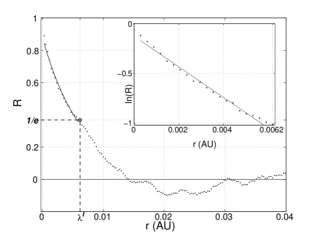
Figure 1: Typical (variance-normalized) magnetic self-correlation function $R$ in the inner heliosphere. This single interval corresponds to Helios 1 observations at $0.964$ AU on December 26, 1974. The inset shows $R$ in logarithmic scale. Solid line shows the linear fit of $\ln(R)$ vs. $r$.

A typical magnetic correlation function, computed by the above method in the inner heliosphere, is shown in Figure 1. We use two different methods, called i and ii, to estimate the magnetic correlation length ($\lambda^{I}$) from the correlation function in each interval. A simple approximation for the behavior of $R^{I}$ at the large scales and in the long-wavelength part of the inertial range is an exponential decay, $R\sim e^{-r/\lambda}$. Method i determines an estimate of the correlation scale $\lambda^{I}_{i}$ as the value of the lag $r$ where the decreasing function $R^{I}$ reaches $\exp(-1)$ by first time, that is $R^{I}(\lambda^{i}_{i})=1/e$. Using the same approximation for the form of the correlation, we can parameterize the correlation function as $\log(R)\sim-r/\lambda$. The second method ii employs this relation and defines $\lambda^{I}_{ii}$ as minus the inverse of the slope obtained from a linear fit to $\log(R)$ vs. $r$ (see inset plot in Figure 1).

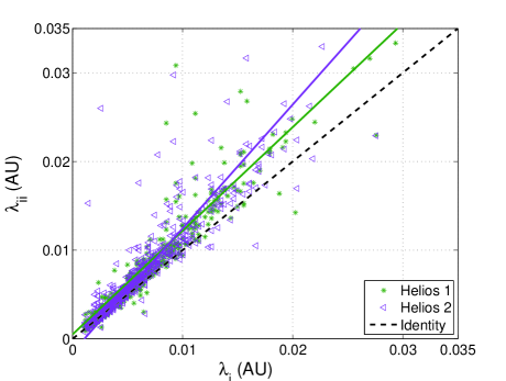
Figure 2: Scatter plot of $\lambda_{ii}^{I}$ vs. $\lambda_{i}^{I}$ for Helios 1 and Helios 2. The line $\lambda_{ii}^{I}=\lambda_{i}^{I}$ and linear least-squares lines are shown for reference.

A comparison of methods i and ii is shown in Figure 2. On average $\lambda^{I}_{ii}$ provides an estimate that is slightly larger than the one provided by $\lambda^{I}_{i}$, $\lambda^{I}_{ii}/\lambda^{I}_{i}\sim 1.16$, as revealed by least-squares fits to the Helios data.

We also include in our data set the mean within each interval of the distance from the Sun to the spacecraft ($D^{I}$), the proton speed ($V_{p}^{I}=V_{sw}^{I}$), and the angle ($\theta^{I}$) between the direction of the mean magnetic field $\langle{\bf B}^{I}_{0}\rangle$ and the SW velocity (${\hat{\bf r}}$, which gives the direction of the spatial lag).

As a final step, we refine the analyzed data set by removing outliers of $\lambda^{I}$. Values of $\lambda^{I}$ are considered as spurious if they depart from their means by one standard deviation $\sigma$ toward smaller values of $\lambda$, or by $2\sigma$ toward larger ones. Also considered outliers are those intervals in which the mean-field direction is not well determined. We select intervals with the direction of $\langle{\bf B}^{I}_{0}\rangle$ (and therefore $\theta^{I}$) well established inside the 24-hour interval. Accordingly, we define the quantity $\Delta\theta$ as the difference between the mean angle $\theta$ in the first half and second half of the interval; and retain only those intervals showing low values of $\Delta\theta$, specifically $|\Delta\theta|<30^{\circ}$. After the above refinements, the final data set encompasses $536$ intervals for H1 and $529$ for H2, totaling $1065$ intervals. Although there are several gaps in the Helios data set, the final $1065$ intervals are roughly equi-distributed during the solar cycle and along the spacecraft orbit.

4 Anisotropy

We proceed to analyze the dependence of $\lambda$ upon heliodistance $D$, angle relative to $\langle{\bf B}^{I}_{0}\rangle$, and the age of the turbulence.

We defined three heliodistance ranges (bins), namely, close to the Sun, intermediate distances, and near $1$ AU, each bin having a width of $0.23$ AU ($0.22$ AU) for H1 (H2). We established two angular channels: the parallel channel ($0^{\circ}<\theta^{I}<40^{\circ}$) and the perpendicular one ($50^{\circ}<\theta^{I}<90^{\circ}$). Narrower angular bins were explored, arriving at qualitatively similar results but with larger errorbars (lower number of intervals per bin). Thus, we conclude that widening the angular channels up to $40^{\circ}$ increases the parallel and perpendicular counts without polluting the results. Nevertheless, smaller angular bins have been used in other works when studying power and spectral anisotropies (e.g., Horbury et al., 2008; Wicks et al., 2010) using methods that differ from what we employ here.

We then distribute all the intervals into the spatial bins and angular channels and compute conditional averages of $\lambda$. In this way, for every heliocentric distance bin we obtain eight mean values of $\lambda$: four $\lambda_{\parallel}$ and four $\lambda_{\perp}$. The factor of four is associated with all combinations of the two spacecraft and the two methods.

The relative order between $\lambda_{\parallel}$ and $\lambda_{\perp}$ can be interpreted qualitatively in terms of the relative abundance of the two basic components, quasi-slab and quasi-2D, of the MHD-scale fluctuations. Accordingly, preponderance of the slab-like component with wavevectors mainly parallel to the mean magnetic field $\langle{\bf B}^{I}_{0}\rangle$ is identified by $\lambda_{\parallel}/\lambda_{\perp}<1$, while preponderance of the quasi-2D component, having mainly perpendicular wavevectors, is identified by $\lambda_{\parallel}/\lambda_{\perp}>1$ (Matthaeus et al., 1990; Dasso et al., 2005).

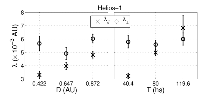
Figure 3: Evolution of $\lambda_{i,\parallel}$ and $\lambda_{i,\perp}$. Left panel: dependence on heliodistance ($D$). Right panel: dependence on turbulence age ($T$). Ticks of the abscissas indicate the center of each bin, bars show the mean’s error.

The left panel in Figure 3 shows the evolution of $\lambda_{\parallel}$ and $\lambda_{\perp}$ with the heliocentric distance for the H1 spacecraft. The data plotted correspond to correlation lengths computed with method $i$ (we obtain similar results with method $ii$ and both methods for H2, not shown here for brevity).

For the group of datasets at distances nearest the Sun, we find that the turbulence is highly anisotropic, with $\lambda_{\parallel}/\lambda_{\perp}=0.58,0.51,0.89,0.81$ for method-spacecraft combinations $i$-H1, $ii$-H1, $i$-H2, $ii$-H2, respectively. As the heliocentric distance grows, the observed anisotropy becomes weaker, due to a steadily growth of $\lambda_{\parallel}$ while $\lambda_{\perp}$ remains nearly constant, implying a shift of $k_{\parallel}$ towards small frequencies, as has been previously reported (Bruno and Carbone, 2005). Several previous works based on observations at $1$ AU have shown that $\lambda_{\parallel}>\lambda_{\perp}$ only for slow SW, as well as for samples with mixed fast and slow SW (Matthaeus et al., 1990; Milano et al., 2004; Dasso et al., 2005; Weygand et al., 2009).

It must be noted that, near the ecliptic plane, the slow wind is much more frequent than the fast wind, and therefore all mean values computed for a mixed SW sample will favor slow SW properties and disfavor fast SW features. In spite of the latter, in the region nearest $1$ AU (ranging from $0.76$ to $0.98$ AU for H1 and from $0.75$ to $0.98$ AU for H2), we find that $\lambda_{\parallel}<\lambda_{\perp}$.

Motivated on result at $1$ AU that shows different relative order between $\lambda_{\parallel}$ and $\lambda_{\perp}$ for fast and slow SW and considering that the high-speed wind will arrive earlier at $1$ AU (and therefore being younger than the slow SW), we analyze the dependence of $\lambda$ on what we call the “age” of the interval. To this end, we compute this age, $T^{I}=D^{I}/V^{I}_{sw}$, for each interval as the nominal time it takes a SW parcel moving at speed ${V^{I}_{sw}}$ to travel a given distance from the Sun to the spacecraft located at $D^{I}$.

Accordingly, we defined three ranges of turbulence age in bins having widths of $20.5$ hours ($19.5$ hours) for H1 (H2). The bin labelled $T_{1}$ is the youngest bin, centered at $40.5$ hours. Bin $T_{2}$ is at intermediate ages centered at $80$ hours, while bin $T_{3}$ contains the oldest samples centered at $120$ hours. In each bin we established the same two angular channels. We compute again conditional averages of $\lambda$, considering only those intervals ${I}$ that correspond to a given angular channel and a given age range, in the same way as described above.

The results taking into account turbulence age, using spacecraft H1 and method $i$, are shown in right panel of Figure 3. Similar results have been obtained using method $ii$ and H2 (not shown). For ages near $40$ hours, that is for the young wind in bin $T_{1}$, we find that $\lambda_{\parallel}\sim\lambda_{\perp}/2$. In particular $\lambda_{\parallel}/\lambda_{\perp}=0.56,0.91,0.48,0.61$, for method-spacecraft $i$-H1, $i$-H2, $ii$-H1, $ii$-H2. This strong anisotropy is consistent with the injection of $k$-parallel Alfvén waves near the Sun. As the wind age grows towards bin $T_{2}$, around the age of $T=80$ hours, we find a trend to an isotropization of $\lambda$. For ages between $T=80$ hours and $T=120$ hours an inversion happens, and when the wind is already old that is for ages about $120$ hours in bin $T_{3}$, we find that $\lambda_{\parallel}>\lambda_{\perp}$, as expected at $1$ AU for a slow or mixed SW. Values of $\lambda_{\parallel}/\lambda_{\perp}$ in each aging bin for the different combinations of spacecraft and method are shown in Table 1, showing robust results.

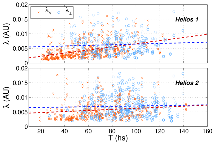
Figure 4: Scatter plot of $\lambda_{\parallel}$ and $\lambda_{\perp}$ vs. age. Here both methods $i$ and $ii$ have been considered. Linear trends are shown for reference: Red line is fit for $\lambda_{\parallel}$; blue line for $\lambda_{\perp}$.

Figure 4 presents as a function of age, and without any binning, the values of $\lambda_{\parallel}$ and $\lambda_{\perp}$ obtained for each interval. Single lines showing linear fits to data (red line for $\lambda_{\parallel}$ and blue line for $\lambda_{\perp}$) reveal a tendency of $\lambda_{\parallel}$ to grow with $T$ at a significantly larger rate than $\lambda_{\perp}$. In fact, with both H1 and H2 datasets it is possible to find a linear behavior of $\lambda_{\parallel}$, which can be represented as $\lambda_{\parallel,s/c}(T)=a_{\parallel,s/c}T+b_{\parallel,s/c}$, where $s/c$ is H1 or H2. Least-squares fits give the coefficients: $a_{\parallel,H1}=(5.3\pm 0.5)\times 10^{-5}$ AU h^-1, $a_{\parallel,H2}=(1.8\pm 0.7)\times 10^{-5}$ AU h^-1, $b_{\parallel,H1}=(1.2\pm 0.3)\times 10^{-3}$ AU and, $b_{\parallel,H2}=(4.4\pm 0.5)\times 10^{-3}$ AU.

In contrast, for $\lambda_{\perp}$, if there is a linear increase, it is apparently so weak that neither H1 nor H2 could observe it, since $a_{\perp,H1}=(1\pm 1)\times 10^{-5}$ AU hs^-1 and $a_{\perp,H2}=(0.6\pm 0.9)\times 10^{-5}$ AU hs^-1, i.e., within error bars the slope may be zero. Nevertheless, a dimensionless global estimator for the evolution of the anisotropy in the range $10<T<200$ hours may be given by the relation: $Q(T)=\lambda_{\parallel}/\lambda_{\perp}=(AT+B)/\langle\lambda_{\perp}\rangle$. Averaging the data from both missions we obtain $A=(3.6\pm 1.7)\times 10^{-5}$ AU hs^-1, $B=(2.8\pm 1.6)\times 10^{-3}$ AU (assigned errors correspond to the semi difference of the Helios values) and $\langle\lambda_{\perp}\rangle=0.007\pm 0.004$ AU.

5 Discussion and conclusions

From the analysis of almost seven years of Helios SW data, we have presented a study of the dynamical evolution of the anisotropy of magnetic fluctuations in the inner heliosphere. The main indicator we employ in this paper for the study of SW anisotropy is the correlation scale measured either mainly parallel to, or mainly perpendicular to, the mean magnetic field direction.

Helios 1 and Helios 2 are unique spacecraft that systematically have in situ observed the inner heliosphere, and therefore they can up to this day provide the best available evidence of the turbulence state close to the Sun, and give hints on the possible initial conditions of the turbulence in the outer corona. The here derived measures of the correlation-scale anisotropy also provide indications relevant for planning the in situ observations by the upcoming Solar Probe Plus and Solar Orbiter missions.

Especially in the inner heliosphere, the state of the turbulence, including the nature of the anisotropies studied here, is a complex combination of boundary and source characteristics. They are related to the initiation of the SW and convolved with various types of evolution that may commence very close to the Sun, perhaps at the Alfvénic critical point (possibly located within 14-34 $R_{s}$; see e.g. Marsch and Richter (1984)). It appears, however, that the observed evolution of the anisotropy with heliocentric distance, as found in this study, is in agreement with several turbulence theories that favor perpendicular spectral transfer of energy. Generally, one expects from experiment, theory and numerical simulations that the anisotropic cascade preferentially magnifies gradients perpendicular to the mean field, while the evolution of the wavevector component parallel to the local mean magnetic field is relatively suppressed (e.g., Zweben and Taylor, 1981; Shebalin et al., 1983; Robinson and Rusbridge, 1971; Oughton et al., 1994; Goldreich and Sridhar, 1995).

The results presented here are consistent with a greater abundance of the slab-like population near Sun, which progressively evolves, according to the SW age, which is defined as the time spent by fluid parcels since their birth near the Sun until the in situ observation. During this evolution, the relative abundance of the slab-like and 2D populations tends to become inverted, and the system reaches at $1$ AU a state resembling that of the slow wind which has a stronger 2D component.

In this work we study the spatial structure of the magnetic correlation function, detecting strong anisotropy near the Sun and weak anisotropy near 1 AU. Power and spectral index anisotropies have also been studied by other authors (e.g., Horbury et al., 2008; Podesta, 2009; Wicks et al., 2010; Narita et al., 2010a, b). These authors have employed methods that effectively define the mean field to be a local quantity that itself depends upon the fluctuations. This way of looking at the anisotropy (based on the local mean field) is very different from the approach used in the present work. Here we treat the mean field as an estimate of an ensemble average quantity, an approach which favors maintaining well defined ensemble averaged directions (i.e., a fixed coordinate system for evaluation of the spectra and correlation functions). Although both methods differ, we view them to be complementary. Examples of the local perspective are given by Cho and Vishniac (2000); Maron and Goldreich (2001); Horbury et al. (2008); Podesta (2009); Wicks et al. (2010). A comparison between the local and global methods is shown by Chen et al. (2011). In particular, Wicks et al. (2010) using $100$ continuous days of Ulysses data reported isotropy of the outer scale for fast polar wind in the outer heliosphere between $1.38$ and $1.93$ AU. On the other hand, Narita et al. (2010a, b), using $4$ hours of Cluster data analyzed the energy distribution of magnetic field fluctuations in the $3$D wave vector domain and obtained direct evidence of the dominance of the 2D picture.

In this manner, our results are fully compatible with earlier findings that the fast SW (which is younger) is more slab-like and that the slow SW (which is older) is more 2D-like (Dasso et al., 2005; Weygand et al., 2011).

These results have direct impact on diffusion models for transport of charged particles through the inner heliosphere, indicating that the energy distribution near the Sun is richer in slab modes than in 2D modes.

Here we have focused on the anisotropy of SW magnetic fluctuations, our future studies will revise the velocity as well as Elsässer-variable fluctuations.

Table 1: Ratios of $\lambda_{\parallel}$ to $\lambda_{\perp}$ for each age bin ($T^{I}$)

Spacecraft	Method	$\frac{\lambda_{\parallel}}{\lambda_{\perp}}$ ($T_{1}$)	$\frac{\lambda_{\parallel}}{\lambda_{\perp}}$ ($T_{2}$)	$\frac{\lambda_{\parallel}}{\lambda_{\perp}}$ ($T_{3}$)
Helios 1	$i$	$0.56\pm 0.05$	$0.89\pm 0.07$	$1.14\pm 0.18$
	$ii$	$0.48\pm 0.06$	$0.77\pm 0.07$	$1.01\pm 0.16$
Helios 2	$i$	$0.91\pm 0.11$	$0.84\pm 0.05$	$0.99\pm 0.10$
	$ii$	$0.61\pm 0.11$	$0.80\pm 0.06$	$0.99\pm 0.11$