Variations in the Mass Functions of Clustered and Isolated Young Stellar Objects

Abstract

We analyze high quality, complete stellar catalogs for four young (roughly 1 Myr) and nearby (within $\sim$300 pc) star-forming regions: Taurus, Lupus3, ChaI, and IC348, which have been previously shown to have stellar groups whose properties are similar to those of larger clusters such as the ONC. We find that stars at higher stellar surface densities within a region or belonging to groups tend to have a relative excess of more massive stars, over a wide range of masses. We find statistically significant evidence for this result in Taurus and IC348 as well as the ONC. These differences correspond to having typically a $\sim$ 10 - 20% higher mean mass in the more clustered environment. Stars in ChaI show no evidence for a trend with either surface density or grouped status, and there are too few stars in Lupus3 to make any definitive interpretation. Models of clustered star formation do not typically extend to sufficiently low masses or small group sizes in order for their predictions to be tested but our results suggest that this regime is important to consider.

1. INTRODUCTION

Does the distribution of masses of stars forming in isolation differ from those forming in clustered environments? The initial mass function inferred from local field stars appears to be consistent with that seen in clusters (e.g., Bastian, Covey, & Meyer, 2010), however, the local field star population is composed of a combination of stars which formed in isolation, stars which dispersed from unbound clusters, and stars which were ejected from bound clusters. Most stars are believed to form in clustered environments (e.g., Lada et al, 2006), therefore stars which formed in isolation or small groups may not be the dominant contributor to the local field star population.

Differences in the distribution of masses of stars forming in clusters versus isolation may be expected, particularly at higher masses. Massive stars are known to form at least primarily within clusters, and it is uncertain both observationally and theoretically whether massive stars can ever form alone. In the competitive accretion scenario, the most massive stars start to form early and spend most of their evolution in high density environments in order to accrete sufficient mass to become a massive star; lower mass stars later form in the gas around the massive stars (e.g. Bonnell et al., 2008). Any massive stars found in isolation would therefore have moved there after accretion or have had their low-mass companions dispersed, rather than having formed in isolation. Under the monolithic collapse scenario, stars form from the fragmentation of their natal core (e.g. McKee & Tan, 2003). Depending on the physical conditions, a massive core could fragment to produce a massive star and / or a group of lower mass stars. Massive isolated stars are therefore not explicitly prohibited from forming by the model, although they may be unlikely. Cores with column densities in excess of 1 g cm^-2, where fragmentation is suppressed (McKee & Tan, 2003), have only been observed in highly clustered environments. In the stationary accretion model of Myers (2009b), massive stars accrete a significant fraction of their mass from the ‘clump’ material beyond their own natal core. To accrete sufficient mass within a sufficiently short time, the clump gas must be denser than in isolated regions. Low-mass stars, on the other hand, could easily form in the surrounding lower density, filamentary distributions of gas; it would be difficult to form a massive star in isolation.

Observationally, few, if any, massive stars appear to have formed in isolation. An upper limit of isolated massive O stars in our galaxy was measured by de Wit et al (2004, 2005) to be $4\pm 2\%$, although this search was limited to massive (O and B star) companions. The apparently isolated O stars may in fact belong to small clusters with lower mass companions, as suggested by the models of Parker & Goodwin (2007).

Clustered star formation appears to extend down to surprisingly small size scales. Kirk & Myers (2011, hereafter Paper I) analyzed fourteen small stellar groupings, typically with 20-40 members, in four young, nearby star-forming regions where deep spectroscopic catalogs are available. Despite possessing surface densities an order of magnitude lower than the standard cluster, Paper I showed that these small stellar groups shared many of the properties associated with clusters. These properties include a correlation of the mass of the maximum mass member with the total group mass, and the central location of the most massive member. The unique advantage of studying clustered star formation in these small stellar groups is the lack of source confusion (due to a combination of the lower source densities and closer distances compared to typical clusters), the inclusion of very low mass members (the catalogs are complete to late M spectral type), and the young age (roughly 1 Myr). Since only approximately half of the stars in each region are identified as belonging to stellar groups, while the other half of the stars are found in relatively isolated environments, these data also provide an excellent opportunity to study differences between the clustered and isolated young stellar populations, in particular the distribution of masses.

Therefore, in this paper we investigate the mass distributions of clustered and isolated populations of young stars. We address the question of whether more massive stars preferentially form in clustered environments. Our main conclusion is that higher mass stars are preferentially found in clustered environments, over a wide range of stellar masses. In order to minimize uncertainties introduced by estimating stellar masses, much of our analysis is performed comparing the spectral types of the stars, which have been accurately measured.

In Section 2, we describe the stellar catalogs and the completeness levels in each. In Sections 3 and 4, we compare the distributions of spectral types for stars in high and low surface density environments (Section 3) and those belonging to groups versus isolated stars (Section 4). We make comparisons to model predictions and various observations in Section 5, discuss the results and interpretations in Section 6, and conclude in Section 7. Stellar motion is analyzed in Appendix A, and several additional statistical tests are discussed in Appendix B.

2. DATA

Currently, four nearby, young star-forming regions (Taurus, Lupus3, ChaI, and IC348) have excellent stellar catalogues with completeness to around 0.02 M_⊙ or type M8.5. The Taurus data was originally compiled in Luhman et al (2010), while the Lupus3 data is a combination of several source lists given in Comerón (2008). In our analysis here, we exclude the six stars which lie at a right ascension of less than 16h 05m and a declination below 39°50′, as we expect the stellar population is incomplete here – this area was covered by only one the source lists in Comerón (2008) (his Table 8). The ChaI data is primarily from Luhman (2007), and the IC348 data is primarily a combination of the catalogs given in Lada et al (2006) and Muench et al (2007). In all cases, the spectral types of the stars were determined spectroscopically, with a typical uncertainty of roughly half a spectal subtype. The total number of stars in each region above the spectral completeness limit is 344 in Taurus, 58 in Lupus3, 215 in ChaI, and 349 in IC348. These data are discussed in more detail in Appendix A of Paper I.

In Paper I, we identified stellar groups based on a minimal spanning tree (MST) analysis. In a MST, all stars are linked together by their nearest neighbours in a tree diagram; groups are defined where all members are connected by separations less than the critical length, $L_{crit}$. Following Gutermuth et al (2009), $L_{crit}$ was determined based on the distribution of all branch lengths. Appendix D of Paper I examines the effect of $L_{crit}$ on the groups identified, and shows that group membership is little affected by variations of $L_{crit}$ within the range of errors expected. In Paper I, we set a minimum group size of more than ten members, based on a visual examination of the MST groupings. Unlike the O-star studies of de Wit et al (2004) and Lamb et al (2010), foreground and background contamination of these catalogues is not a concern, allowing groups to be identified without relying on statistical comparisons with background source density counts.

Masses were estimated based on a combination of stellar evolutionary models by Palla & Stahler (1999), Baraffe et al (1998), and Chabrier et al (2000), and assuming a constant age of 1 Myr. As discussed in Paper I, these assumptions lead to an overall uncertainty in the mass of each star of about 50%; the ranking of the masses is, however, much more certain (and is exact for any single stellar age assumed). Where possible in the analysis here, comparisons are made using spectral types rather than masses to minimize the uncertainties.

2.1. Orion Nebula Cluster

In Paper I, we also compared the properties of the young stellar groups to those of a typical young cluster. For this purpose, we analyzed the ONC dataset of Hillenbrand (1997). There, our MST algorithm identified one very large cluster (the central cluster where the Trapezium stars are found), as well as five small stellar groups with properties similar to those found in the four nearby star forming regions. In Paper I, we considered only the large ONC cluster for comparison, as it alone represented typical cluster properties.

For the ONC cluster identification and analysis in Paper I, we included only sources listed with a 70% or higher ‘probability of membership’ (based on proper motion observations) in Hillenbrand (1997). We used this conservative cut to prevent potential contamination by non-ONC members. Many of the fainter sources in Hillenbrand (1997), however, did not have proper motion data available at the time, and hence had no probability of membership measure. Hillenbrand (1997) estimated that the majority of sources without proper motion data were likely bona fide cluster members, based on the fraction of known members as a function of both the separation from the cluster centre and spectral type.

A comparison of the properties of isolated and clustered stars could be strongly sensitive to variable completeness, both spatially and spectrally. In order to avoid any potential bias in our results for the ONC, we therefore run our analysis on two versions of the ONC catalog. The conservative proper motion-cut catalog analyzed in Paper I will be referred to as ONC-c; additionally, we analyze the full ONC catalog with no cuts applied, which will be denoted as ONC-f. The former should have minimal contamination from non-ONC stars, but an irregular completeness at later spectral types, while the latter catalog has better completeness but a higher likelihood of contamination. We ran the same group-identification algorithm on both ONC catalogs separately; due to the higher surface density, ONC-f has a smaller $L_{crit}$ than ONC-c: $L_{crit}$(ONC-f) is 0.08 pc and $L_{crit}$(ONC-c) is 0.13 pc.

Hillenbrand (1997) estimated that their optical catalog contained roughly half the total number of cluster members (the others being detected only in the infrared due to high extinction), and that the optical sample was representative of the full distribution both in terms of spatial distribution and spectral types. Sixty percent of the optical sample had spectral types measured, with a roughly uniform completeness level both spatially and as a function of I and V band photometry (assumed to roughly correlate with spectral types). While the spectral type determinations are therefore not complete, Hillenbrand (1997) argue that they should be representative of the full population in every respect. The ONC survey completeness is roughly 14.5 mag in K-band and 17.5 mag in I band in the least-sensitive part of the survey Hillenbrand (1997), which corresponds to roughly a mass of 0.04 to 0.055 M_⊙ at an age of 1 Myr or 0.06 to 0.075 M_⊙ at 5 Myr. We adopt a conservative estimate of a spectral completeness limit of M6.5.

In general, we find similar results using either the ONC-c or ONC-f catalog, suggesting the completeness is reasonably consistent in the ONC-c catalog.

3. DISTRIBUTION OF SPECTRAL TYPES IN HIGH VERSUS LOW SURFACE DENSITY ENVIRONMENTS

3.1. Calculating the Local Stellar Surface Density

In order to compare the properties of stars inhabiting isolated versus clustered environments, a scheme to classify each is required. One simple method which does not rely on the definition of stellar groups is to use the local stellar surface density, $\Sigma$. If the separation from the star to its $n$th nearest neighbour (where $n$ is 1 for the star itself) is $r_{n}$, then the local surface density is

$$\Sigma=\frac{n-1}{\pi r_{n}^{2}}~{}~{}~{}.$$ (1)

As discussed in Gutermuth et al (2009) and Casertano & Hut (1985), the fractional uncertainty in $\Sigma$ varies as $(n-2)^{0.5}$; higher values of $n$ give a lower spatial resolution, but smaller fractional uncertainty. Bressert et al (2010) recently used this surface density measurement to argue that there is no distinct scale for YSO clustering within nearby star-forming regions.

We calculate $\Sigma$ for each star using both $n=4$ and 9, to allow us to examine the dependence on $n$. Since Paper I found many examples of stellar groups with roughly ten to twenty members, $n$ values larger than about 10 would have poor sensitivity to this clustering, while $n$ values of two or three could bias surface density measures for close visual pairs or binary stars.

3.2. Comparison of Spectral Type Distributions

We examine whether there is a global preference for earlier spectral types at higher $\Sigma$. Ordering all YSOs within each region by $\Sigma$ (for $n=4$ and 9), we compare the spectral type distributions for the upper and lower thirds of the population. Figures 1 to 3 show a comparison of the cumulative spectral type distributions for the $n=4$ case for each of the four regions, as well as the ONC for comparison. Each plot shows the cumulative fraction in both linear space (main plot) and log space (inset), to highlight differences as the later and earlier spectral types respectively. Comparisons are only made for stars above the completeness levels discussed in Section 2 and with known spectral types, as are all subsequent measures in this paper. The error bars in the figures denote the Poisson $\sqrt{N}$ error for each point. Three of the regions – Taurus, IC348, and the ONC – show striking differences between the high and low surface density stars. These regions show an overabundance of stars at earlier spectral types in the high surface density environment versus the low surface density environment. This is not only the case at the earliest spectral types, but extends throughout nearly the entire range of spectral types in the sample. Statistical tests described below confirm this visual impression. The results of the statistical tests are given in Table 1. Similar trends, but with poorer statistical significance were found comparing the upper and lower $\Sigma$ halves of the population, likely because stars at intermediate values of $\Sigma$ have similar properties, but are distributed in both bins.

3.3. Statistics

We ran three statistical tests on the distributions of spectral types for the grouped and isolated stars to quantify the differences visually suggested in Figures 1 to 3. The first two of these tests examine global differences between the stars in high and low surface density environments, which will therefore be weighted where the bulk of the stars are, i.e., the later spectral types. The final test focusses on the differences solely at early spectral types.

3.3.1 Kolmogorov-Smirnov test

We first ran a two-sample Kolmogorov-Smirnov (KS2) test; the KS2 test provides an effective way to measure whether two datasets are statistically similar, i.e., whether it is likely that both are drawn from the same distribution. The KS2 test is sensitive to differences in the datasets’ medians and variances (Conover, 1999). Table 1 shows the KS2 probabilities that the high and low surface density stars share a common distribution of spectral types. The KS2 test suggests that the high and low surface density stars are distinct at the 95% or higher confidence level with either $n=4$ or 9 in IC348 and in the ONC, while in Lupus3, the populations are consistent with being drawn from the same distribution at the 96% confidence level, likely due to the small number of stars in that region. ChaI has intermediate KS2 probabilties and so does not fall definitively into one or the other category. Taurus shows a strong difference in populations for $n=4$ (95% confidence level), but not for $n=9$, suggesting that very small stellar groupings are significant in the spatial distribution of stars in Taurus.

We ran similar comparisons between stars in high and low surface density environments with more severe (earlier) completeness levels assumed, and find similar KS2 values for completeness levels of 3-5 spectral subtypes higher in nearly every region, for both the $n=4$ and 9 surface density measures. The one exception is the ONC-c catalog, where KS2 values remained low only for a completeness level of up to two spectral subtypes earlier than what we assumed.

The KS2 test does not have a formal mechanism to include measurement errors in the calculation. In order to assess the effect of uncertainty in the spectral types on the KS2 test statistic, we therefore ran a series of trials with random errors added to the measured spectral types. For each entry in Table 1, we ran 10,000 trials with added spectral type uncertainties of half a subtype, and calculated the resulting KS2 test statistic. This is summarized in Table 2, and demonstrates that the significant KS2 test statistics are robust to uncertainty at the expected level. Systematic biases in the spectral types measured are not expected as a function of spatial clustering or spectral type (K. Luhman, private communication).

3.3.2 Mann-Whitney

While the KS2 test is an excellent way to determine whether two distributions are different, it does not provide a measure for how they differ, e.g., if one of the distributions tends to have extra high- or low- valued members. To address this, we ran a second statistical test, the Mann-Whitney (MW) test, also known as the Wilcoxon test (Conover, 1999). In this test, two datasets are compared based on their relative ranking (i.e., the ordering of the values of both datasets combined); tied values are each assigned the average rank of the ties. The basic premise of the test is that two sets of data drawn from the same overall distribution will have roughly equal total ranks, whereas if one data set tends to have higher values, then the total of its ranks will tend to be lower (since a rank of 1 denotes the largest value). The MW test probability that the high surface density stars tend to have earlier spectral types than the low surface density stars is given in Table 1 for each region. We emphasize that the MW test is most sensitive to differences in the range of spectral types where the bulk of the stellar populations are, i.e., earlier spectral types refers primarily to those at the late-type end, around M-type. Taurus, IC348, and the ONC show high probabilities that the stars in high surface density environments tend to have earlier spectral types. Both Lupus3 and ChaI have no strong evidence that either the higher or lower surface density stars tend to be of earlier spectral type.

Where differences are seen in the spectral type distributions, we can make a rough estimate of this typical difference. We apply a global shift to the spectral types of the low surface density stars, and measure how large an offset may be added so that the MW test shows negligible statstical significance that the high surface density stars tend to have earlier spectral types. We find that required shifts in the spectral types are quite small - shifting all of the low surface density stars earlier by between half and one spectral subtype is sufficient for the MW test to return probabilities of 85% or smaller that Taurus, IC348, and ONC stars have earlier spectal types in high surface density environments.

As with the KS2 test, we ran the same statistical comparisons varying the assumed completeness level of the sample, and found the same result, i.e., the conclusions drawn from the MW test remain unchanged for completeness levels up to at least two spectral sub-types earlier than assumed.

Uncertainties in the spectral types measured also do not have an impact on the MW test statistic – we ran a similar test to that described in the previous section for the KS2 test, and find little variation in the MW test statistic (see Table 2).

3.3.3 Early Type Stars Counting Test

Neither of the above tests explicitly focusses on differences specifically in the early type star populations at high and low surface densities. There are an insufficient number of stars in each region (save the ONC) to run the above two tests only on the early type stars in each environment. Instead, we must rely on a simpler statistical test, comparing the total number of early type stars in high and low surface density environments. If the populations were identical, roughly the same number of early type stars should be found in the high and low surface density samples, since the total number of stars in each is equal. To determine whether the differences are significant, we compare the value to the Poisson error in the number of early type stars in the low surface density sample. We then define the excess of early type stars in the high surface density environment as

$$\begin{array}[]{rcl}E_{early}&=&\frac{N_{early,high~{}sd}-N_{early,low~{}sd}}{\sqrt{(\sqrt{N_{early,high~{}sd}})^{2}+(\sqrt{N_{early,low~{}sd}})^{2}}}\\ &=&\frac{N_{early,high~{}sd}-N_{early,low~{}sd}}{\sqrt{2N_{early,low~{}sd}}}\\ \end{array}$$ (2)

which gives roughly the number of sigma of significance.

The value of $E_{early}$ depends on what spectral type is used as the early type cutoff. Since it is not obvious, a priori, what spectral type should be used, we performed the calculation for a range of cutoffs, every half a spectral type from late G to early B, in order to see what type(s) would give the highest statistical significance to the difference. Table 1 gives the maximum value of $E_{early}$ we found, and the early type cutoff spectral type or types that it was found for. The four nearby regions tend to have $E_{early}$ values of $<2\sigma$ with an early type cutoff of around G0. The ONC had much higher $E_{early}$ values, from 3 to 8 $\sigma$, when a very early type cutoff, around B5, was used.

3.3.4 Statistics Summary

In summary, we find that there are statistically significant differences between the spectral types of stars found in low and high surface density environments in IC348 and the ONC, as well as Taurus, when small stellar groupings are considered (using $n=4$). In these regions, the higher surface density stars have an overabundance of earlier spectral types compared to the lower surface density stars. This overabundance corresponds to an average spectral type which is half to one spectral subtype earlier for the high surface density stars. There are too few stars in Lupus3 to show any statistically significant differences, while the ChaI stars do not follow the general trend. Focussing only on the early type stars, none of the four nearby regions have a sufficient number of stars to show statistically significant differences in the populations. Significant differences are seen, howevever, in the ONC, as has also been noted in previous studies (e.g., Hillenbrand & Hartmann, 1998).

3.4. Combined Distribution

Finally, we examine the spectral type distributions for the combination of all four regions. Combining the spectral type distributions may increase the statistical significance of the difference between the high and low surface density environments, since all regions but ChaI visually follow the same trends. Merging the individual spectral type distributions can be done in two ways. The first method is to add together the spectral types for all of the YSOs classified as high surface density in their individual regions, and similarly for the low surface density stars. This is shown in the top panel of Figure 4, and the resulting statistical measures are given in Table 1. The appearance is qualitatively similar when stars in ChaI are excluded, however, the statistical significance of the trends is slightly higher in this instance (these numbers are also given in Table 1).

On the other hand, the data from the four regions can also be combined by splitting up the stars into those falling in the upper and lower global thirds of the surface densities measured in all four regions. This would be the more appropriate combination method to adopt if the mechanism driving the difference between environments was dependent on the absolute surface density of stars. The bottom panel of Figure 4 shows the combined spectral type distributions split by absolute surface density. Note that each region populates a different fraction of the high and low surface density cuts; Taurus YSOs dominate the low surface density cut, while IC348 YSOs dominate the high surface density cut. The difference between the spectral type distributions using the two combination methods is striking. While both show an excess of early type stars in the higher surface density environment, the size of the difference and the range of spectral types over which the difference is present are both smaller when the global surface density cut was applied. The smaller range of the excess has a significant effect on the KS2 and MW statistics measured, since much of the population is at later spectral types where the difference between high and low surface densities is diminished.

The fact that combining the data from the four regions using the relative surface density cuts rather than a global cut shows a much larger difference between the two populations suggests that the mechanism responsible for the difference at high and low surface densities operates in a relative sense, rather than coming into effect at a set absolute surface density value. It is interesting to note that the global surface density comparison shows a much stronger difference when Taurus rather than ChaI stars are excluded from the sample, despite Taurus stars on their own showing a difference while ChaI stars do not. This appears to be the case because Taurus’s early type stars, which are in relatively higher surface density environments within Taurus, are classified as being in low surface density environments in comparison to surface densities seen in the other regions.

4. DISTRIBUTION OF SPECTRAL TYPES IN GROUPS VERSUS ISOLATION

A second way to compare the stars is to subdivide the stars in each region into those that were found to belong to an MST-defined stellar group in Paper I and those that were not associated with a group. As discussed in Section 2, groups are defined as having more than ten members with nearest neighbour separations less than $L_{crit}$; stars not associated with a group (‘isolated stars’) are therefore all stars which are connected to fewer than ten sources with separations of $L_{crit}$ or less. Figures 5 to 7 show the cumulative fraction of sources earlier than a given spectral type for each of the four regions as well as the ONC for comparison, using the same plotting conventions as Figure 1.

Unlike the comparisons at high and low surface densities, the grouped versus isolated cumulative distributions tend to show significant differences over more localized spectral types. IC348 in particular, and Taurus to a lesser extent, appear to show an excess of later-type stars (mid-M) in the groups, and this also appears in the ONC. The main difference between the two ONC catalogs is the stars in groups with spectral types around F. Hillenbrand (1997) found that stars around type F were the most likely to have small proper motion membership probabilities; if proper motions were preferentially measured for stars nearer the centre of the ONC, then our ONC-c catalog would have a deficit of F stars in groups versus isolation compared to the full ONC-f catalog, as Figure 7 shows.

4.1. Statistics

We ran the same statistical comparisons as discussed in Section 3 on the grouped and isolated stellar distributions. These results are summarized in Table 3.

In general, we see similar results to the statistical tests for the high versus low surface density stellar distributions, although with generally slightly poorer statistical significance. We again verified that the spectral completeness limits adopted do not affect the results, for completeness levels at least 2-3 subtypes earlier than we assumed.

Here, to compare the number of the early type stars in groups verus isolation, we first correct for the total number of stars in each category. The number of early type stars expected to be found in groups, based on the number of early type stars found in isolation, is

$$N_{early,grp,exp}=N_{early,isol}\times\frac{N_{tot,grp}}{N_{tot,isol}}$$ (3)

and the excess of early type stars in groups over that expected from the isolated population is analogous to equation 2, but using the full error propogation required from equation 3.

Similar to the high and low surface density populations, we find relatively small excesses of early type stars. The excesses are typically smaller than for the high and low surface density populations, since the extra step of normalizing the total sample sizes increases the associated error measure. Here, the largest magnitude of excess in ChaI is actually a deficit of early type stars in groups, although at less than 1$\sigma$ significance. The ONC stars again show the most significant excesses of early type stars in the groups, but only at the $\leq 2\sigma$ level. We tested the effect of measurement uncertainty in the spectral types using the same procedure as outlined in Section 3.3.1. The results, listed in Table 4, show that the KS2 and MW test statistics are robust to the spectral type error.

In summary, similar to the surface density comparisons, the tests show that IC348 and the ONC have statistically significant differences between the spectral types of stars in groups versus isolation. In Taurus, IC348, and the ONC, stars in groups have a global tendency to be at earlier spectral types than stars in isolation, again with a high statistical significance. This tendency is not obvious when examining only the earliest spectral types (with the $N_{early}$ test), likely due to small number statistics. The trends seen in these three regions tend to be slightly statistically weaker than those seen comparing the high and low surface density environments, and may be more pronounced at localized spectral types. Lupus3 again does not have a sufficient number of stars to see a statistically significant difference, and ChaI does not appear to follow the general trend.

4.2. Combined Distributions

Similar to Section 3.4, we also compare the distribution of stellar spectral types for stars in and outside of MST groups in Taurus, Lupus3, ChaI, and IC348 combined. This data is shown in Figure 8, and the corresponding KS2 and MW statistics are given in Table 3. As expected, combining the data from the four regions tends to enhance the trends seen, as is also apparent in the statistical measures. Excluding the stars in ChaI, where no trend is apparent, has little effect on the qualitative appearance of Figure 8, but does slightly further strengthen the statistical measures.

4.3. Individual Taurus and ChaI Groups

While the populations of grouped stars are dominated by a single clustered environment in both IC348 and the ONC, and only one group was identified in Lupus3, in the Taurus grouped population, there are comparable contributions from eight different stellar groups. Here, we examine each group independently to determine whether our conclusions change when groups are treated separately. Similarly, we compare the three groups identified in ChaI, noting that there, one of the groups dominates the total number of sources by a factor of two.

The number of stars in each group above the spectral completeness limit ranges from fourteen to thirty one in Taurus, and from twelve to eighty three in ChaI, which are small sample sizes to search for statistically significant differences. Nevertheless, we compared the KS2 and MW test statistics for each group individually versus all of the isolated stars in the region. These statistics are given in Table 5. Results from the $N_{early}$ test are not shown, as none of the groups have a statistically significant excess of early type stars at the earliest spectral types, due to the small number of sources in each group.

Most of the Taurus groups have KS2 probabilities indicating the single group and isolated stars are statistically indistinguishable, and MW probabilities that neither population has a strong tendency for more massive members. Surprisingly, two Taurus groups did show strong global differences with the isolated population, despite the small number of members. Both Taurus Groups 4 and 5 (L1551 and L1529) have KS2 probabilities of less than 10% and MW probabilities of $\gtrsim 90\%$, implying that overall the stars in these groups tend to have earlier spectral types than the isolated population. The spectral type distributions of the exceptional Taurus Groups 4 and 5 are shown in Figure 9.

Group 5 / L1529 is a small group, with its most massive member only of spectral type K5, and shows a substantial excess of sources relative to the isolated population around type M0. Group 4 / L1551, on the other hand, is a somewhat larger group, with a B9 / B9.5 pair of stars, and shows a systematic offset of more massive stars at all spectral types. In Paper I, L1551 was one of only two groups which did not have a centrally-located most massive member – the B9 and B9.5 stars fall near the outskirts of the group. L1551 therefore is only an exemplar for the differences seen in the spectral type distributions in groups and isolation, and not also the location of the most massive member. In Paper I, we noted that had the group been defined with a slightly smaller $L_{crit}$, the B9/B9.5 stars would not have been considered group members, and the next most massive member is centrally- located. Interestingly enough, if the B9/B9.5 stars were excluded from the L1551 spectral type distribution, the grouped and isolated stars would still show a systematic difference – the absence of the two B9/B9.5 stars is not sufficient to make the two distributions agree.

Conversely, we test whether the excess of earlier type stars is confined to only these two groups in Taurus. We compare the spectral type distributions for the stars in all groups except groups 4 and 5 and the isolated stars, and find a diminished, but still visible, excess of early type stars in groups. This excess only extends down to about type K0, and is sufficiently small that the KS2 and MW tests do not yield significant results. This appears to indicate that the bulk of the difference in the grouped stars populations arises from only a few of the groups, although there are hints that the difference is present at a lower level in at least some of the other groups.

In ChaI, each individual group appears much more similar to the isolated distribution; none of the groups have the striking visual appearance of differences that are seen in Figure 9. ChaI Group 2 has a relatively low KS2 probability that the grouped and isolated stars are similar (12%); this appears to be caused by a slight deficit of grouped stars at mid-M spectral types versus the isolated distribution.

4.4. Distribution of Spectral Types with Varying Group Size

Our analysis in Section 4.1 distinguishes groups and isolated stars assuming that groups must have more than ten members. The MST group identification scheme used in Paper I, however, identifies all groupings of stars which are separated by less than $L_{crit}$, and therefore identifies groupings as small as pairs of stars. The minimum group size is somewhat arbitrary, chosen in Paper I to allow for the measurement of mass segregation. In light of the fact that very small groupings of stars may be important, particularly in Taurus (Section 3), it is useful to examine various minimum group sizes. A visual examination of the YSOs suggests that a significant fraction of the earliest type stars not found in our $N>10$ MST groups are instead found within smaller MST groupings; there are relatively few early type stars which do not belong to any size of MST grouping.

We re-ran the statistical comparisons discussed in Section 4.1 on grouped and isolated stars using different minimum group sizes. The details are discussed in Appendix B; the overall conclusion is that the definition of a group does not have a strong influence on the differences seen between the grouped and isolated stellar spectral types. Increasing the minimum group size substantially causes some of the genuine groups to be classified as isolated sources, diluting the difference between the two populations. Decreasing the minimum group size has a small effect on the statistical measures until the minimum group size is so small that few stars are categorized as isolated and the ability to statistically distinguish the two populations is poor. Table 6 shows the results for the same statistical tests as given in Table 3 but with a minimum group size of $N\geq 2$ and $N\geq 15$. As in Section 3, the stars in Taurus show the largest increase in the KS2 probability with an increase of the minimum group size, suggesting that stellar clustering on small scales is important in this region.

5. DISTRIBUTION OF MASSES

Comparison between our observations and other observations, in addition to predictions from clustered star formation models are more easily made using the distributions of mass, rather than spectral types. As illustrated in Sections 3.4 and 4.2, the distribution of spectral types combined over the four nearby star-forming regions offers a reasonable representation of the trends seen in the individual regions, with a generally higher statistical significance due to the greater number of stars compared. For simplicity in mass space, we make comparisons only of these combined datasets. Note that for the surface density comparison, we use the combination displayed in the top panel of Figure 4, i.e., each region contributes an equal number of YSOs to the high and low surface density populations.

As discussed in Paper I, our simple method of assuming a constant stellar age tends to introduce biases in the mass distribution. To better understand this effect, we made comparisons of the mass distributions shown in Luhman et al (2009) for Taurus, ChaI, and IC348 versus the mass distribution which we would derive using the same basis set of spectral types and a constant 1 Myr age. We find that the assumption of a global 1 Myr age tends to cause an overestimation of the number of the most massive stars in each region (around 2 M_⊙ and above), and hence an accompanying underestimate of the number of slighly less massive stars; there is also a smaller prevalent overestimate of the number of stars with around 0.2 M_⊙, and a similar underestimate at slightly lower masses. Assuming a constant age of 2 Myr instead, we find significantly improves our mass estimations above $\sim$1 M_⊙; we could not find a single age estimate to improve the smaller bias at the lower mass end. For our analysis of the mass distributions we therefore revise our masses above 1 M_⊙ to be those predicted assuming an age of 2 Myr, which slightly reduces the values. We stress that our mass distributions should still be viewed as approximate estimations, given our simple age assumption.

Figure 10 shows the cumulative mass distribution for the regions, overlaid with predictions from several models (more details below). The differences between the populations are less visually apparent than in Figures 4 and 8; the difference is entirely due to the variable stretch in the conversion from spectral to mass space, since a single conversion between spectral type and mass is assumed. The bumps in the mass distribution are likely due to inaccuracies in our assumed conversion. Note that despite the visual appearance, our statistical tests provide the same results in mass-space as spectral type-space, since we assume a one-to-one translation between the two. To quantify the typical mass difference between the two distributions, we ran a similar MW shift test to that described in Section 3.3.2, finding the shift which, when applied to the low surface density or isolated stars, returns an MW probability of $\sim$85%. We found that for both Taurus and IC348, the high surface density stars are typically 18% more massive than the stars in low surface density environments, while stars in groups are 4% and 11% more massive than their isolated counterparts in Taurus and IC348 respectively.

For comparison, Figure 11 shows the corresponding plots for the ONC-c catalog; the ONC-f catalog appears similar. In the ONC, the mass estimates are expected to be more accurate, since Hillenbrand (1997) allowed the stellar ages to vary when estimating the masses. Applying the same MW shift test as above, we find that the stars in high surface density environments are roughly 8% more massive than the stars in low surface density environments, while the stars in groups are 6% more massive than their isolated counterparts.

5.1. Effect of Single Age on Statistics

The statistics discussed above were calculated assuming a constant stellar age, however, variations in the stellar ages could affect the values quoted. Here, we discuss additional tests to investigate this effect.

5.1.1 KS2 and MW Test Statistics

As noted above, with the assumption of (any) constant stellar age, the KS2 and MW test statistics are identical to those found for the spectral type distributions, since there is a one-to-one mapping between the two. Allowing for age variations could change the shape of the mass distributions. In particular, having systematically older stars the more clustered environments would tend to decrease their masses, and therefore lessen the difference seen between the more and less clustered populations (i.e., high versus low surface density or grouped versus isolated). We ran tests varying the stellar ages adopted for the clustered stars to determine the age difference size necessary to make the two populations appear similar. Assuming that the less clustered population is 2 Myr old, then we find that the more and less clustered populations can match at the very high mass tail (stars above $\sim$2 M_⊙) only when the more clustered stars are $\sim$5 Myr old. Even this large an age difference, however, is insufficient to decrease the excess of more massive stars in the more clustered population in the $\sim$0.2 - 2 M_⊙. This remains true even if the less clustered population is reduced to an age of 1 Myr. Since stellar evolution tracks run roughly vertically for masses below of order 1 M_⊙, changes in age have almost no impact on the stellar masses inferred from the spectral type.

Since age thus primarily affects only the highest mass stars which are few in number, the KS2 and MW statistical tests are largely impervious to systematic changes in age. For any reasonable assumption about ages, the KS2 test statistic remains small (5% or less) in all cases where it was small under the assumption of a global constant age. Age has a slightly higher, but still small, effect on the MW statistic. In Taurus, the MW statistic drops by less than 2% for more clustered stars which are 1 Myr older than the less clustered stars; only when the more clustered stars are set to 5 Myr while the less clustered stars are 1 or 2 Myr does the MW statistic drop below 90% in some cases. Even in this drastic case, the MW statistic for the $n=4$ surface density comparison only changes from 99% to 98%. In IC348, the effect is slightly larger, due to a greater number of sources at the higher mass ranges which are effected by the age assumed. Still, the MW test statistic drops by at most a few percent when the more clustered stars are $\leq$ 1 Myr older than the less clustered stars. All of the IC348 MW test statistics remain above, and normally well above, 90% while the more clustered stars are younger than 5 Myr.

5.1.2 Mass Shift Values

We find that the mass shift values quoted are only very weakly dependent on the stellar ages assumed. We ran similar comparisons between the more and less clustered stars, and found that the mass shifts were roughly identical for any constant age adopted for both popuations. If the more and less clustered populations have ages different by less than 0.5 Myr, again the mass shifts measured remain virtually unchanged. For more clustered stars which are older (/younger) by 1 Myr, the mass shifts are decreased (/increased) by at most 2%.

5.1.3 Summary

The statistical results presented for the mass distributions are largely insensitive to variations in the age assumed, despite age being a strong factor of uncertainty in the absolute values of the masses estimated. In order to decrease the statistical significance of the results presented in this section, stars would need to be systematically and noticeably older (a $>$ 1 Myr difference) than stars in the less clustered environments. There is no clear physical mechanism which would cause more clustered stars to be systematically older by such an amount. In fact, clustering is often seen to be tighter for younger stars than older ones (e.g., Luhman et al, 2010). Systematically younger stars in clusters would tend to strengthen our statistical measures and would tend to increase the mass shift measured between the more and less clustered environments.

5.2. Comparison to Model Predictions

Here, we compare the observed cumulative distribution of masses to two recent model predictions – the first, analysis of competetive accretion simulations in Maschberger et al (2010, hereafter M10), and the second, analytic predictions by Krumholz et al (2010, hereafter K10) based on the monolithic collapse scenario.

5.2.1 Competitive Accretion Simulations

M10 analyzed the clustering properties of stars (represented by sink particles) formed in the competitive accretion simulations of Bonnell et al. (2008) and Bonnell et al. (2003), with a focus on the evolution of clusters and their most massive members. Clusters were identified using the MST formalism, with $L_{crit}$ set to 0.025 pc through visual inspection and a minimum size of thirteen members. For comparison, in Paper I, we determined $L_{crit}$ based on the distribution of branch lengths, with $L_{crit}$ ranging from 0.52 pc in the more dispersed Taurus stars to 0.083 pc in the more tightly clustered IC348. The M10 critical length for highly clustered simulations therefore seems reasonably consistent with our definitions; the minimum number of group members is also similar.

M10 found that about 60% of all sources form within clusters, and of those sources, most tended to form with the same radial distribution as already existed in the cluster. The most massive sources (defined as any source with a final mass greater than about 1 M_⊙), on the other hand, tended not to form in clusters – rather, clusters tended to later form around a pre-existing massive source. Often, this started out as a small ‘sub-cluster’, which then successively merged with other small ‘sub-clusters’, and eventually formed a massive cluster, with the massive stars from each sub-cluster ending up in the centre of the final system. This evolution occurred rapidly, as the simulations were only run for 0.5 Myr.

At the end of the Bonnell et al. (2008) simulation, the distribution of masses of sink particles found within groups / clusters and in isolation and the fits listed in Table 1 of M10. The sink particle masses are upper limits to the masses expected in the stars – the authors noted that effects such as stellar feedback and binary fragmentation were not included in the simulation, and would serve to decrease the resultant stellar mass. With that caveat, Figure 10 shows the sink particle mass distributions in M10 overlaid on the observed stellar distributions. M10 only measure the mass distributions down to 0.8 M_⊙, which corresponds to roughly 15% of the total number of sources in all of our observations; the lines plotted show the M10 results scaled down by this factor.

A comparison between the scaled-down M10 distributions and the observed ones show that the two are in reasonable agreement, given both the small number statistics (and estimated mass uncertainty) in the observations, as well as the errors M10 estimate in their mass function parameters (not plotted). It is also interesting to note that the M10 results show a substantial distinction between the clustered and isolated sinks, with most of the massive sinks being found in clusters. We observe a much smaller difference between the stars in groups and isolation. It is possible, however, that some processes which can reduce the final stellar mass from that in the simulated sink particles (such as stellar feedback) operate more strongly in a clustered environment, which would decrease the difference between the two M10 curves.

5.2.2 Monolithic Collapse

An analysis similar to M10 has not yet been performed for the monolithic collapse scenario, making a direct comparison to our observations challenging. The best available predictions are from K10, who construct several simple analytic models to describe the distribution of final stellar masses based on results from several star formation simulations which include radiative feedback.

Based on both the simulations and a prior theoretical prediction (Krumholz & McKee, 2008), K10 find that in high density environments (above $\sim 1$ g cm^-2), fragmentation of massive dense cores is largely inhibited, allowing for the formation of massive stars. In lower density environments, fragmentation occurs much more regularly, leading to smaller stellar masses arising from a given core. These results were used as the basis for an analytic model in K10 which predicts the final distribution of stellar masses formed in both high and low density environments. K10 assume the initial dense core mass distribution follows the Chabrier (2005) IMF, scaled up by a factor of three, and a star formation efficiency for any core fragment of a factor of 1/3. In the high density case (model ‘fH’), they assume no fragmentation, i.e., each core forms one star, and the mass distribution mirrors the Chabrier (2005) IMF. In the low density regime (‘fL’), several different cases of fragmentation are considered, with varying amounts of mass in each fragment.

The high and low density regimes of the K10 models do not have a direct corresponendence to our observations, as the spatial distribution of high and low density cores was not specified in the model. While a direct comparison therefore cannot be made, the observed distribution of masses for grouped and isolated stars should fall within the range spanned by the models. Figure 10 shows the range spanned by the K10 models at 1 and 10 M_⊙. (Note that these models span all masses, and do not require normalization for comparison with observations as the M10 measurements do.)

The most noticeable feature of the K10 models is that the fraction of stars expected at 10 M_⊙ and above is relatively high for both low and high density environments. All of the K10 models predict more stars at 10 M_⊙ and above than even the M10 distribution for groups; the K10 range lies well above the observed value for the four nearby star-forming regions, and is barely consistent with the high surface density / grouped stellar population (only) in the ONC. The predicted fraction of massive stars in the K10 models could be decreased by assuming a smaller maximum core mass, or, in the low density case, by assuming either a smaller fraction of the mass forms the main source, or that the core fragments into a larger number of pieces.

5.3. Comparison to Field Star MF

Finally, we compare to observed mass functions. Mass functions are often presented in differential form, i.e., number per mass bin, so we follow that convention here. Figure 12 shows the differential mass function for high and low surface density stars (top panel) and grouped and isolated stars (bottom panel). The general tendency is for the high surface density stars to be more numerous than the low surface density stars at the upper mass end, and the reverse at the low mass end. Similarly, the grouped stars tend to be more numerous than the isolated stars at high mass, and less numerous at low mass. This common behaviour is more prominent for stars at high and low surface density than for stars in groups and isolation, as was seen earlier.

We note that inaccuracies due to our assumption of a constant stellar age are more apparent in differential than cumulative form. In Figure 10, assuming an age of 1 Myr or 2 Myr when estimating the masses above 1 M_⊙ creates barely discernable differences in cumulative mass distributions. In the differential mass distribution, however, there is a noticeable shift of objects from the highest mass bin to the second highest mass bin when the ages are assumed to be older. Most of these stars which shift bins have masses little above the boundary between the two bins with an assumed age of 1 Myr; our bin sizes and boundaries were chosen to match those in Luhman et al (2009) to facilitate easier comparison between the two.

Keeping in mind that the estimated masses are still somewhat uncertain, we compare the distribution of masses in the four nearby star-forming regions to the field star mass function. The field star mass function provides an approximate measure of the current, nearby isolated star-forming population. These stars are expected to have formed over a range of times, and therefore at the present day will be somewhat depleted of their higher-mass members, relative to the initial mass function. Furthermore, the field star population is expected to consist of a combination of stars which formed in isolation, with those that formed in small groups or clusters that have since dispersed or ejected some of their members. The field star mass function would thus be expected to be formed from a combination of our more and less clustered stellar populations.

Figure 12 shows the Reid et al (2002) field star mass function, corrected for the effects of stellar evolution (their Figure 14, bottom panel); this field star mass function spans a larger range in masses than some more recent observations such as Covey et al (2008). The evolution-corrected field star mass function is consistent, within errors, with other determinations of the IMF (Reid et al, 2002). While the mass distribution of the stars in high surface density environments appears to be skewed to slightly higher masses than the Reid et al (2002) field star mass function, they are consistent within errors. The low surface density, grouped, and isolated stellar mass distributions all appear to be in closer agreement with the Reid et al (2002) field star mass function; the largest discrepancy is around 0.2 M_⊙, where we earlier noted our mass estimates were biased relative to those where a range of ages are used.

5.4. Maximum Versus Total Group Mass

Another property of the groups examined in Paper I was the relationship between the mass of the most massive group member and the total group mass. In large clusters, the mass of the maximum mass member and the total cluster mass are correlated (e.g., Weidner et al, 2010). At high masses, the flattening of the relationship between maximum and total mass was interpreted as evidence that a maximum stellar mass exists. At lower masses, the relationship has a constant slope which is roughly consistent with the relationship expected for cluster members randomly sampling the IMF, although Weidner et al (2010) find that the scatter in the cluster data is smaller than expected for pure random sampling. We showed in Paper I that the relationship between maximum and total mass continues to the smallest of the groups we identified. Here, we examine whether the trend is also present in even smaller grouping of stars, and whether there is a minimum group size at which the correlation is seen.

The top panel of Figure 13 shows the relationship between maximum and total stellar mass for all groupings of six or more stars in Taurus, Lupus3, ChaI, and IC348, while the bottom panel shows the same relationship for groupings of two or more stars. In both panels, the grey diamonds show the cluster data compiled by Weidner et al (2010), while the coloured circles show the stellar groupings we identified with the MST. The dotted line shows the approximate relationship fit by Weidner et al (2010) at low cluster masses, which provides a reasonable description of the groups as well. This continues to agree well with the smaller groupings, all the way down to pairs of stars.

While the small groupings follow the trend remarkably well, it is worth nothing that the range of values they can span becomes increasingly restricted at lower group sizes. The dashed line indicates a 1-1 relationship, the upper limit for any group size, representing all mass residing in the most massive group member. For every number of group members, there is also a lower limit, with a slope of the inverse of the number of members; this lower limit lies parallel and below the 1-1 line on the plot. Even with this consideration of the smaller range possible for small groupings, the correlation between the maximum and total cluster mass is quite good, which suggests that properties of stellar groups may extend to systems with fewer than ten members. This could be interpreted as evidence that the masses of stars in the small groupings are consistent with a random sampling of the IMF or an IMF-like distribution, even though the total number of members is too small to measure this directly. Higher accuracy mass estimates would be needed to determine the consistency of the scatter in the data with that expected from pure random sampling.

6. DISCUSSION

In clustered regions, the tendency to find more massive stars in regions of higher surface density is linked to mass segregation, since higher surface densities correspond to smaller cluster-centric radii. Hillenbrand & Hartmann (1998) observed mass segregation in the ONC for stars with masses above 1-2 M_⊙ at all radii, and some evidence for mass segregation at even smaller masses in the inner radii; a more recent analysis of the ONC data with a MST-based technique has found strong evidence of mass segregation only down to 16 M_⊙, with weaker evidence of mass segregation down to 5 M_⊙(Allison et al, 2009). Similarly, mass segregation has been observed for IC348 (e.g. Muench et al, 2007). In Paper I, we analyzed mass segregation from the perspective of the groups, and found that the most massive group member, and in a few cases, also the second most massive group member, tended to be centrally located, reminiscent of mass segregation.

In this work, we extend the analysis to include stars not in groups, and find that the differences in mass distributions apply not only to clusters, but also to dense and sparse groups. This tendency suggests a kind of “mass enrichment” associated with stellar surface density, but not “mass segregation” due to location within a group. We find that massive stars tend to be more prevalent in higher stellar surface density environments and within stellar groupings, well below the surface densities typically associated with clusters. Perhaps the most surprising result is that this trend is not only strong in IC348 and the ONC where it had been previously observed, but is also seen in the relatively dispersed stellar population of Taurus. Given the tendency for more massive sources to be found in more clustered environments in both the clustered IC348 and the dispersed Taurus regions, it is puzzling that a similar trend was not seen in ChaI, whose environment appears to be intermediate between these two extremes. Two of the three groups identified in ChaI did, however follow the general trend found it Paper I of having a centrally-located most massive group member.

Stellar motion is the final piece of the puzzle not yet examined. Since all of the regions are quite young, the stars should not have had a chance yet to move a significant distance away from their birth sites. We consider the available proper motion data for all of the early type stars in our sample to verify this assumption in Appendix A. Within the current observational uncertainties, there is no evidence for stellar motion to have influenced our results.

How do the differences in the stellar distributions in more versus less clustered environments arise? Are more low mass stars preferentially born in lower density environments, or are they former members of small groups that were cast out at an early age? Our data show suggestive signs that the excess in massive stars in more clustered environments may not be a uniform excess, but may be clustered around several spectral types, specifically an excess of late B types and late K types, corresponding to masses around 3 and 1M_⊙ at 1 Myr. If this observation were borne out in a larger dataset with higher statistical significance, that would suggest that a more complicated physical process related to formation mechanisms is responsible. It is difficult to see how a simple picture of ejection, for example, would have such specific preferred mass scales. If instead there is a roughly uniform excess of massive stars in more clustered environment, this could be more easily attributed to the formation process. The fact that many stars form in a group suggests that the group environment has advantageous conditions relative to the field environment, such as a gas resevoir which allows for higher accretion rates or longer accretion timescales, which would be favourable for forming higher mass stars.

The differences seen between the masses of clustered and isolated young stellar objects suggests that the initial mass function (IMF) is not independent of the physical conditions of star formation. Differences in the IMF may not always be so apparent, as the primary contributions are likely to be from the most ‘successful’ star-forming regions, i.e., more clustered environments.

7. CONCLUSION

Complementary to the analysis presented in Paper I, we compare the more and less clustered populations of stars found in four nearby young star-forming regions – Taurus, Lupus3, ChaI, and IC348. The clustered young stellar population in the ONC is also used as a comparison. We find the following results:

1. Stars in the most clustered of regions, IC348 and the ONC, have statistically significant differences between the populations associated with high and low surface density and also with groups and isolation. The stars in high surface density environments or groups tend to be skewed overall to more massive members at the 98% or higher confidence level. These statistics are driven by by differences in the populations at the low-mass end, although differences are seen out to the earliest spectral types as well. The typical difference in masses between the high surface density or grouped stars and the low surface density or isolated stars is $\sim$11-18% in IC348.

2. Despite being the classic example of isolated, distributed star formation, the stars in Taurus follow the same trends as the clustered regions. Stars in higher surface density environments in Taurus tend to have larger masses than the lower surface density environment stars at the 99% confidence level, and stars in groups tend to have larger masses than those found in isolation at the 96% confidence level. These statistics are again primarily driven by differences in the populations around spectral type M, although differences are seen at the earliest spectral types. The typical difference in masses between the high surface density or grouped stars and the low surface density or isolated stars is $\sim$4-18%.

3. The Lupus3 catalog is not large enough to allow for any strong conclusions to be made.

4. ChaI does not follow the trends seen in the other regions, and shows no evidence for more early type stars in grouped or higher surface density environments. In Paper I, two of the three groups in ChaI did follow the general trend of a centrally-located most massive member, however.

5. The combined mass distribution from all four regions is consistent to what is observed in the evolution-corrected field star mass function, or, similarly, the IMF.

6. In all four regions, the relationship between the mass of the most massive group member and the total group mass seen in clusters and larger groups continues to arbitrarily small group sizes.

7. Stellar motion does not appear to be responsible for the ejection of all the isolated early type stars, given the young ages of the star-forming regions, and the large separations of some of the early type stars from any stellar groupings.

The complete stellar catalogues available for these four nearby star-forming regions allow the properties of stars in small groups and isolation to be quantified to an extent not previously possible. Although theories of massive and clustered star formation tend to focus on large, high density systems, our results suggest that small, relatively sparse, nearby regions offer an alternative regime in which to test the models. The deep, uniform completeness levels and lack of contamination and source confusion allow for the characterization of grouped and isolated sources at a level not possible in more distant clusters.

Appendix A PROPER MOTION

The current YSO positions must be assumed to be similar to their birth locations in order to attribute the differences in stellar populations to the star formation process. Significant stellar motions are known to occur in some systems, however. In large clusters, the ejection of even relatively massive members is seen in numerical simulations (e.g., Vine & Bonnell, 2003), and in observations (Goodman & Arce, 2004). Smaller, sparser systems better corresponding to our stellar groups are less well-studied. N-body simulations of very small groups (with N$\sim$5) including the effects of gas accretion and drag indicate that single stars up to one fifth the mass of the total group mass can be ejected early in the group’s evolution (Delgado-Donate, Clarke, & Bate 2003; see Kiseleva et al 1998 for the case of no gas). Bate, Bonnell, & Bromm (2003) furthermore argue that larger dynamical perturbations occur for both single stars and binaries in larger systems where larger-scale star-star interactions occur. Despite the young age and low stellar surface density in our star-forming regions, these simulations suggest that stellar motions should be examined to determine if they have could have effected the currently observed YSO positions.

We examine the likelihood of significant stellar motion for the earlier type stars in our sample, both from a theoretical perspective of the necessary energetics (Appendix A.1) and using the available proper motion data (Appendix A.2). For ease of analysis, we divide the YSOs into our standard $N>10$ groups, and consider only the motion of the early type stars. The groups in general have good correspondence to high surface density environments, so the results should be generally applicable. Due to their fewer numbers, the migration of a single early type star would have a larger impact on the resultant distributions than a later spectral type star; observationally, proper motions are only available for the brightest stars.

A.1. Theory

A.1.1 Movement Out of Groups

We first examine the likelihood that the isolated early type stars formed within their nearest group and subsequently migrated to their current locations. The escape speed required to leave each group is roughly

$$V_{esc}=\sqrt{\frac{2GM_{tot}}{R}},$$ (A1)

where $M_{tot}$ is the current total mass of the group, and $R$ is the separation from the group centre from which the star would start its migration. We consider for two cases for $R$ – a star forming at a ‘typical’ group separation, or $R_{rms}$, the standard deviation of all current group member separations, and a star forming at the group outskirts, or $R_{max}$, the current maximum group member separation. The values of $R$ and $V_{esc}$ for each group are given in Table 7.

For each isolated early type star, we calculate the star’s separation to both the centre and outskirts of its nearest group, using the separation to the closest group member as a proxy for the latter. For IC348, separations only to the main cluster are considered, since it strongly dominates the dynamics of the region; Lupus3 has no isolated early type stars, and is not considered. The separations are listed in Table 8; for stars 1 Myr old, each separation (in pc) is approximately equal to the velocity (in km s^-1) required to move that distance. The ratios between the velocity required to reach the group centre or edge and the associated escape velocity are also given in Table 8, along with whether each star is more massive than all of the current group members. Figure 14 shows the separations of all isolated early type stars in Taurus from their closest group centre (top panel) and group outskirts (bottom panel) in right ascension and declination, with darker shades indicating earlier spectral types. The mean values of $R_{max}$ and $R_{rms}$ for all of the groups in Taurus are shown in the bottom left corner of the top panel. The concentric annuli indicate separations of 0.5, 1, and 2 pc respectively. The other regions show similar behaviour, with some early type stars well-separated from the nearest group, and others located much closer.

Quantitatively, for a plausible dynamical ‘ejection’ from the group, the isolated star should be less massive than the most massive member currently in the group, and the velocity required to take the star to its current location (assuming an age of 1 Myr) should not be substantially larger than the escape speed for the group. With these considerations, we see that all of the isolated early type stars in IC348 could have moved to their current locations, as well as few of the G stars in Taurus and ChaI. Taurus-312, Taurus-352 and ChaI-209 and Cha-210, all appear too isolated and / or massive to be potential migration candidates. We stress that the migration candidate stars undoubtedly include a significant fraction which did not undergo migration. Our simple analysis uses only separations on the plane of the sky, while the 3D separation could be much larger. Even if the 3D separation is reasonable for migration, it does not mean that migration necessarily occured. Further constraints using available proper motion data are given in Appendix A.2.

A.1.2 Movement Into Groups

For completeness, we also look for indications that the early type stars currently in groups migrated there after forming in isolation. Table 9 gives the separation between each star and the group centre and edge, along with whether it is the most massive member of its group. As was found in Paper I, the early type stars tend to be found near the centre of their group, making it unlikely that they migrated there in only a $\sim$1 Myr timescale. A few stars, such as Taurus-350 and Taurus-351 are the most likely candidates to have formed either outside the group, or on the outskirts of the group.

A.2. Proper Motion Data

We now use proper motion measurements in conjunction with the theoretical considerations above to constrain the likelihood of stellar migration.

To find the proper motion of each star, we searched the recent all-sky proper motion catalogs of Zacharias et al (2010), Röser et al (2010), Röser et al (2008), van Leeuwen (2007), Zacharias et al (2004), and Kharchenko (2001). In a non-negligible number of sources, the proper motion listed for the same source in multiple catalogs differed by more than the errors listed. In IC348, Zacharias et al (2010) list a subset of the stars as moving with a substantially different proper motion in RA ($\sim$25 mas yr^-1) than is given in the other catalogs (most give negative values). In order to minimize bias from discrepant catalogs, we use a two-step process to estimate the ‘best’ proper motions for each early type star, and caution that these values are still highly uncertain. We first calculate the median proper motion for each star, and then eliminate all measurements which differ by more than 15 mas/yr from this value (the quoted errors are typically much smaller than this). With the remaining measurements, we calculate the weighted mean (weighting by the error of each measure), which we will refer to as the ‘best’ value, and error. We also calculate the range spanned by all of the measures remaining after the first step; this range of ‘good’ proper motion measures provides a more realistic sense of the possible range in values than the formal error. Tables 10 and 11 list the ‘best’ proper motion, associated error, and range of possible values for the early type stars found in isolation and groups respectively. Note that the proper motion measurements are all given relative to each star’s nearest or associated group.

The proper motion of each early type star needs to be considered in relationship to the nearest or associated group. Table 7 lists the proper motion we adopt for each group. In Taurus, we use the values given in Luhman et al (2010); the Luhman et al (2010) proper groups generally match well with the groups we identify, although both our Groups 2 and 3 match the same Luhman et al (2010) group. For Lupus3 and ChaI, the group proper motions have been calculated in the same manner as for Taurus but are not yet published (E. Mamajeck, priv. comm., Mar 9, 2011). No statistically significant differences were seen for the stars in the northern and southern parts of ChaI, so the value for the entire population is used. A similar proper motion measurement has not yet been made for IC348, so we estimate this value using the weighted mean of the individual ‘best’ proper motions we calculate for group members; the error given is the standard error.

A.2.1 Movement Out of Groups

We estimate where each isolated star would have been 1 Myr ago relative to its nearest group, using the range of good proper motion values. The range of possible positions is often quite large; we list the smallest separation from the group in this range, $Sep_{1Myr}$, in Table 10 to indicate whether the star could possibly have originated from the group, given the available proper motion data. In IC348, the results are particularly uncertain, given both the larger scatter between measurements discussed earlier, as well as the small angular scale spanned by the stars (small relative motions have a larger impact on the final relative position). Given these caveats, we see that about half of the isolated early type stars have proper motions consistent with having originated in a group, while the other half do not. Including the theoretical considerations in Appendix A.1, the stars which appear to be the most promising candidates for migration are Taurus-97, ChaI-91, and all of the stars in IC348 barring IC348-7 and IC348-11.

A.2.2 Movement Into Groups

We similarly estimate where each grouped early type star would have been 1 Myr ago relative to its current group; these values are given in Table 11. Note that since $Sep_{1Myr}$ measures the predicted minimum separation to the group centre 1 Myr ago, small, but non-zero values are consistent with the star being a group member in the past. With this consideration, the only stars whose proper motions suggest they formed outside the group and migrated in are Taurus-58, Taurus-351, Lupus3-22, Lupus-23, ChaI-154, and IC348-18.

Upon closer consideration of the data, all of these sources appear to be consistent with originating in their current groups. Proper motion measurements consistent with group membership are found for both Taurus-58 and Taurus-351 in catalogs which were excluded from the ‘good’ values (Röser et al (2008) and Kharchenko (2001) respectively); Taurus-351 is also a binary star, which may contribute to the discrepancy between catalogs. The range of good proper motion measures for both of the Lupus3 stars, ChaI-154, and IC348-18, are nearly compatible with the group’s proper motion; given the scatter between catalog values, it seems likely that the errors are somewhat underestimated.

A.3. Summary

Significant stellar motion appears unlikely for most of the early type stars in our sample. A precise determination is difficult, given the large uncertainties in the proper motion measurements, the unknown line of sight distances, and precise ages of the stars. Isolated early type stars in IC348 have the highest likelihood of having originated in a group, since this region is the most compact and tends to have the most uncertain proper motion measurements. In Taurus and ChaI, a few G-type stars currently found in isolation are the most likely candidates for having formed in a group. None of the stars currently in groups show compelling evidence for having formed in isolation and migrating inward. The sources which may belong to a different category than when they formed compose a small number of the total number of early type sources, and have primarily slightly later spectral types, where the total number of sources is larger. Our statistical analyses are therefore expected to remain similar even with proper motion considerations.

Notably, the isolated F0 and B6.5 stars in ChaI appear unlikely to have originated in a group, suggesting that, while rare, some massive young stars may indeed form in isolation.

Appendix B EFFECT OF GROUP DEFINITION

In Section 4, stars were classified as belonging to a group or being in isolation based on the stellar groups defined in Paper I, i.e., stellar groups needed more than ten members, each separated from their nearest neighbour by less than the critical length $L_{crit}$. We examine the effect of adopting a different minimum number of members to define ‘grouped’ and ‘isolated’ YSOs in Appendix B.1 and B.2, and finally, using a different $L_{crit}$ in B.3.

B.1. Smaller Groups

We re-run our comparisons of grouped and isolated YSO spectral types using minimum group sizes of $N\geq$10, 8, 6, 4, and 2. We tend to find similar statistical results for the smaller minimum group sizes, with the variation increasing at the smallest group sizes. Table 6 gives the KS2 and MW probabilties for a minimum group size of $N\geq 2$. The grouped and isolated stars in ONC are clearly still distinct with this drastic change in group defintion. In Lupus3 and ChaI, as before, the probabilities do not allow us to make definitive conclusions. In IC348, the grouped and isolated populations appear to be much more similar with $N\geq 2$ than $N>10$, which appears to be due to the small number of stars which are classified as isolated (the grouped stars are nearly seven time more numerous than the isolated stars in this instance). For $N\geq 6$, the KS2 and MW statistics are in better agreement with the standard $N>10$ case. In Taurus, the populations of grouped and isolated stars actually appear to be more distinct for $N\geq 2$ than with $N>10$. This is in agreement with the finding in Section 3 that small groupings of stars in Taurus are distinct from the truly isolated stars.

B.2. Larger Groups

Conversely, we examine the effect of increasing the minimum group size. Since there are few groups of any given size, we examine minimum group sizes of $N\geq 15,20,25,40,$ and 55, chosen to match the discrete group size values in our sample. These values also encompass group sizes in which the number of grouped and isolated sources are roughly equal, minimizing the statistical uncertainty in comparisons. The grouped and isolated source counts are closest for $10<N\leq 16$ (Taurus), $12<N<36$ (ChaI), $11<N<186$ (IC348), $37<N<410$ (ONC-c), while in ONC-f, $N<10$ would be required. Lupus3 has only one group with $N>10$, so cannot be tested for an increase in the minimum group size.

Table 6 shows the KS2 and MW probabilities for $N\geq 15$. As the minimum group size, $N$ is increased, the KS2 probabilities that the ‘grouped’ and ‘isolated’ spectral types are drawn from the same parent distribution tend to increase slowly with small increases in $N$, and then rapidly increase once a significant fraction of the original $N>10$ grouped stars become classified as ‘isolated’. This transition tends to occur at or slightly below the value of $N$ which makes the number of sources classified as grouped or isolated roughly equal. From this, we conclude that a slight increase of the minimum group size does not have a significant impact on our results. Increasing the minimum group size significantly ($\sim$20 or higher, depending on the region), however, serves to wash out the differences seen between grouped and isolated sources.

B.3. Different $L_{crit}$

$L_{crit}$, the maximum separation between group members, is the second variable which controls whether sources are classified as belonging to a group or not. In Paper I, we found an uncertainty of $\leq$ 10% in $L_{crit}$, using the definition in Gutermuth et al (2009) for $L_{crit}$. Appendix D.1 of Paper I examined the effect of a varying $L_{crit}$ on group membership, and found typically only a handful of late type stars would be included or excluded from all of the groups in a region with a different $L_{crit}$. Changes much larger than the measurement error (at least 40-60%, but usually at least double the measured value) are required to cause significant changes to the classification of sources. We therefore conclude that the choice of $L_{crit}$ does not have a strong influence on the resulting spectral type distributions or the statistical measures that we present.

Table 1Statistics for YSOs separated by surface density

	n = 4						n = 9
Region	KS2	MW	Eearly		Median $\Sigma$		KS2	MW	Eearly		Median $\Sigma$
	(%)	(%)	max $\sigma$	cutoff	low	up	(%)	(%)	max $\sigma$	cutoff	low	up
Taurus	5	99	1.4	G0,A0	0.65	44.0	54	92	1.4	G0,A0	0.61	15.8
Lupus3	96	75	1.4	G9-G0	1.80	154	96	62	1.4	G9-G0	2.56	125
ChaI	25	32	0.7	A5,A0	4.95	140	25	25	1.5	G9	4.97	138
IC348	3	99	3.5	G0	48.3	667	0.3	98	1.8	G0	48.2	491
ONC1-c	0.1	99.97	4.9	B5	28.0	379	0.005	99.995	3.0	B5	27.7	276
ONC1-f	0.8	98	7.1	B5	38.7	977	5	90	7.8	B5	37.4	910
Combined	0.6	99.8	3.5	G0	—	—	5	97	2.4	G0	—	—
T+L+I	0.2	99.98	4.5	G0	—	—	1	99	2.4	G0	—	—
Combined global	68	55	4.1	G0	2.72	285	0.08	0.1	3.5	G0	2.24	234
T+L+I global	28	57	5.3	G0	2.24	345	6	29	4.1	G0	2.02	292
L+C+I global	9	98	6.5	G0	10.9	425	22	91	6.0	G0	11.3	339

Table 2Effect of Spectral Type Uncertainty on Surface Density Statistics

KS2 Statistic
	n = 4			n = 9
Region	median	90th percentile		median	90th percentile
	(%)	(%)	(%)	(%)	(%)	(%)
Taurus	8	4	11	54	34	76
Lupus3	96	46	96	96	74	96
ChaI	60	25	96	60	25	96
IC348	3	0.8	8	0.5	0.1	2
ONC1-c	0.05	0.02	0.1	0.003	0.001	0.007
ONC1-f	0.6	0.3	1	3	2	6
Combined	0.7	0.2	2	6	2	14
T+L+I	0.2	0.05	0.7	1	0.5	4
MW Statistic
Taurus	99	99	99.6	92	89	94
Lupus3	75	60	96	62	48	74
ChaI	35	26	45	27	19	36
IC348	99	98	99.5	98	96	99
ONC1-c	99.96	99.9	99.98	99.99	99.98	99.997
ONC1-f	97	95	98	88	83	92
Combined	99.8	99.6	99.9	98	96	99
T+L+I	99.97	99.9	99.99	99	99	99.7

Table 3Statistics for Grouped and Isolated YSOs

Region	KS2	MW	$E_{early}$
	(%)	(%)	max $\sigma$	cutoff
Taurus	32	96	1.4	G0
Lupus3	95	38	1.4	G9-G0
ChaI	11	12	-0.4	G0
IC348	0.8	98	1.2	G9
ONC1-c	0.02	99	1.2	B5
ONC1-f	6	86	2.0	B5
Combined	5	94	1.5	G9
T+L+I	1	99	1.8	G0

Table 4Effect of Spectral Type Uncertainty on MST Group Statistics

	KS2 Statistic			MW Statistic
Region	median	90th percentile		median	90th percentile
	(%)	(%)	(%)	(%)	(%)	(%)
Taurus	28	14	47	96	94	97
Lupus3	89	48	99.7	38	26	53
ChaI	28	9	63	15	9	22
IC348	0.2	0.04	0.8	98	96	99
ONC1-c	0.2	0.04	0.9	99	99	99.6
ONC1-f	5	3	9	85	79	90
Combined	8	4	19	95	92	97
T+L+I	2	0.6	5	99	99	99.7

Table 5Statistics for Individual Groups in Taurus and ChaI

Region	Group	KS2	MW
		(%)	(%)
Taurus	1	60	64
Taurus	2	88	67
Taurus	3	71	48
Taurus	4	3	99.8
Taurus	5	8	89
Taurus	6	99	67
Taurus	7	73	83
Taurus	8	54	61
ChaI	1	42	10
ChaI	2	12	5
ChaI	3	46	72

Table 6Statistics for Groupings and Isolated YSOs with $N\geq$ 2 and $N\geq 15$

	$N\geq 2$		$N\geq 15$
Region	KS2	MW	KS2	MW
	(%)	(%)	(%)	(%)
Taurus	7	95	42	90
Lupus3	37	13	95	38
ChaI	19	68	23	26
IC348	17	63	0.3	98
ONC1-c	0.8	91	0.8	98
ONC1-f	0.02	81	0.4	98

Table 7Group Properties

Region	Grp	Rrms	Rmax	Vesc(Rrms)	Vesc(Rmax)	$\mu_{\alpha}$	$\mu_{\delta}$	$\Delta\mu$	Refs
	#	(pc)	(pc)	(km s-1)	(km s-1)	(mas/yr)	(mas/yr)	(mas/yr)
Taurus	1	0.24	0.82	0.62	0.33	6.9	-22.3	1	L10
Taurus	2	0.29	1.13	0.68	0.34	6.0	-26.8	1	L10
Taurus	3	0.40	1.31	0.42	0.23	6.0	-26.8	1	L10
Taurus	4	0.35	1.38	0.75	0.38	10.0	-17.6	1	L10
Taurus	5	0.23	0.69	0.56	0.32	5.5	-21.9	1	L10
Taurus	6	0.42	1.64	0.60	0.30	6.7	-17.7	2	L10
Taurus	7	0.48	1.85	0.54	0.27	4.5	-21.3	2	L10
Taurus	8	0.26	0.88	0.64	0.35	3.9	-23.4	1	L10
Lupus3	1	0.24	1.06	0.80	0.38	-9.4	-21	1.1	EM1
ChaI	1	0.16	0.48	0.44	0.26	-20.9	1.3	0.7	EM2
ChaI	2	0.21	1.01	1.27	0.59	-20.9	1.3	0.7	EM2
ChaI	3	0.17	0.61	1.04	0.55	-20.9	1.3	0.7	EM2
IC348	1	0.13	0.58	2.73	1.29	5.6	-6.6	0.8	KM
IC348	2	0.04	0.15	0.79	0.43	5.6	-6.6	0.8	KM

Table 8Required Motions for Isolated YSOs

Region	Src	Spec.	Closest	Separation	Separation	V/Vesc	V/Vesc	$M<$
	#	Type	Grp	Centre (pc)	Edge (pc)	Centre	Edge	$M_{max}?$
Taurus	97	G5	2	1.69	0.84	2.53	2.49	Y
Taurus	160	G8	6	2.50	0.95	4.26	3.20	Y
Taurus	233	G8	4	1.35	0.86	1.83	2.34	Y
Taurus	312	G5	4	9.77	8.51	13.29	23.16	Y
Taurus	352	A2	8	2.19	1.67	3.49	4.92	Y
ChaI	91	G9	3	0.63	0.23	0.62	0.43	Y
ChaI	209	F0	1	2.56	2.21	5.95	8.87	N
ChaI	210	B6.5	3	1.38	0.92	1.35	1.70	N
IC348	3	A0	1	0.94	0.44	0.35	0.35	Y
IC348	7	A0	1	0.49	0.18	0.18	0.14	Y
IC348	8	A2	1	0.48	0.17	0.18	0.14	Y
IC348	11	G4	1	0.76	0.50	0.29	0.39	Y
IC348	17	A4	1	0.93	0.44	0.35	0.35	Y
IC348	19	G1	1	0.64	0.37	0.24	0.29	Y
IC348	21	G5	1	0.87	0.50	0.32	0.39	Y
IC348	25	A4	1	0.62	0.37	0.23	0.29	Y

Table 9Required Motions for Grouped YSOs

Region	Src	Spec.	Group	Separation	Separation	$M=$
	#	Type		Edge (pc)	Centre (pc)	$M_{max}?$
Taurus	58	B9	2	1.01	0.12	Y
Taurus	255	G0	6	1.27	0.36	Y
Taurus	287	G5	7	1.44	0.40	Y
Taurus	328	B9	8	0.68	0.20	Y
Taurus	336	G2	8	0.62	0.26	N
Taurus	350	B9.5	4	0.43	0.95	N
Taurus	351	B9	4	0.43	0.95	Y
Lupus3	21	A7	1	1.03	0.03	N
Lupus3	22	A3	1	1.02	0.03	Y
ChaI	11	G5	2	0.43	0.58	N
ChaI	53	B9	3	0.47	0.13	Y
ChaI	116	G2	2	0.63	0.37	N
ChaI	121	B9.5	2	0.63	0.38	N
ChaI	154	G8	2	0.27	0.74	N
ChaI	182	G7	2	0.87	0.13	N
IC348	1	B5	1	0.51	0.07	Y
IC348	2	A2	1	0.48	0.10	N
IC348	4	F0	1	0.34	0.23	N
IC348	5	G8	1	0.16	0.41	N
IC348	6	G3	1	0.37	0.20	N
IC348	9	G8	1	0.47	0.10	N
IC348	10	F2	1	0.37	0.20	N
IC348	12	G0	1	0.33	0.24	N
IC348	13	A3	1	0.33	0.24	N
IC348	16	G6	1	0.54	0.04	N
IC348	18	A2	1	0.48	0.10	N
IC348	28	F0	1	0.30	0.27	N
IC348	29	G1	1	0.12	0.45	N
IC348	35	G0	1	0.32	0.25	N
IC348	359	B5	1	0.51	0.07	Y
IC348	360	G8	1	0.47	0.10	N

Table 10Observed Relative Motions for Isolated YSOs

Region	Src	$\mu_{\alpha,B}$	$\Delta\mu_{\alpha,B}$	$\mu_{\delta,B}$	$\Delta\mu_{\delta,B}$	Min $\mu_{\alpha}$	Max $\mu_{\alpha}$	Min $\mu_{\delta}$	Max $\mu_{\delta}$	Sep1Myr
Taurus	97	1.63	1.14	-1.05	1.13	-1.08	4.02	-3.90	1.15	0
Taurus	160	-5.70	4.60	-27.33	4.58	-32.19	2.12	-44.29	-21.18	14.6
Taurus	233	-13.26	2.42	9.61	2.42	-15.68	-10.84	7.19	12.03	9.6
Taurus	312	2.66	1.19	-1.70	1.19	-0.11	4.70	-3.29	0.04	5.9
Taurus	352	1.25	1.09	-1.53	1.10	-0.97	3.09	-4.29	0.28	0
ChaI	91	-0.40	1.11	1.11	1.04	-3.87	3.11	-2.81	5.97	0
ChaI	209	-5.78	0.80	-11.47	0.72	-7.19	-4.53	-13.29	-8.79	6.4
ChaI	210	-1.90	0.73	0.12	0.67	-3.50	-0.63	-0.91	1.30	0.2
IC348	3	-2.30	0.93	0.48	0.68	-3.94	3.94	-2.09	1.41	0
IC348	7	2.78	1.16	-1.93	1.00	0.76	5.55	-5.31	-0.01	1.6
IC348	8	-0.04	1.16	-0.69	0.98	-1.63	2.38	-5.42	1.23	0
IC348	11	-8.38	4.84	-4.04	4.80	-22.45	-2.74	-18.90	1.72	4.6
IC348	17	-2.54	5.45	-2.10	4.41	-30.92	3.76	-10.62	34.51	0
IC348	19	-5.34	2.74	-0.66	4.70	-9.10	2.26	-8.32	15.31	0
IC348	21	-5.49	2.27	2.90	4.04	-8.14	1.16	-7.02	20.05	0
IC348	25	-1.45	3.83	-0.16	4.01	-6.76	4.06	-8.82	9.62	0

Table 11Observed Relative Motions for Grouped YSOs

Region	Src	$\mu_{\alpha,B}$	$\Delta\mu_{\alpha,B}$	$\mu_{\delta,B}$	$\Delta\mu_{\delta,B}$	Min $\mu_{\alpha}$	Max $\mu_{\alpha}$	Min $\mu_{\delta}$	Max $\mu_{\delta}$	Sep1Myr
	#	(mas yr-1)		(mas yr-1)		(mas yr-1)		(mas yr-1)		(pc)
Taurus	58	-27.15	8.12	-2.02	4.26	-39.47	-15.06	-8.10	9.73	10.1
Taurus	255	4.71	2.21	3.73	2.21	1.49	7.56	-0.22	6.90	0.6
Taurus	287	-2.90	6.23	1.60	6.23	-9.13	3.33	-4.63	7.83	0
Taurus	328	-1.68	1.13	-1.17	1.06	-3.35	1.24	-2.93	0.25	0.03
Taurus	336	0.79	1.26	-0.25	1.19	-5.78	3.22	-3.75	3.04	0
Taurus	350	-2.95	1.44	-0.64	1.11	-6.76	2.33	-3.36	1.87	0
Taurus	351	15.20	2.09	-1.66	1.49	12.41	17.99	-6.41	2.05	7.7
Lupus3	21	0.18	1.17	-2.91	1.17	-1.69	4.44	-7.43	-0.96	0.9
Lupus3	22	3.10	1.18	-1.22	1.16	0.91	5.42	-3.25	0.25	0.9
ChaI	11	2.26	1.01	-1.79	1.78	0.51	7.48	-4.75	1.18	0.8
ChaI	53	-0.54	0.84	-1.91	0.76	-1.99	1.46	-3.29	0.48	0
ChaI	116	-3.29	1.36	3.06	1.28	-5.65	0.38	-1.04	8.05	0
ChaI	121	1.42	0.78	0.41	0.71	-0.75	3.25	-1.37	1.77	0
ChaI	154	-0.69	1.20	3.52	1.17	-1.89	0.51	2.35	4.69	1.4
ChaI	182	-0.44	2.73	6.66	2.38	-10.15	8.87	-11.21	16.71	0
IC348	1	-1.03	1.15	-0.15	0.97	-8.04	0.64	-6.77	16.71	0
IC348	2	1.39	1.44	0.23	1.32	-2.02	3.95	-4.46	2.56	0
IC348	4	2.52	1.21	-0.24	0.87	-4.74	5.30	-2.31	2.56	0
IC348	5	-1.25	3.73	-2.51	3.60	-8.96	6.26	-13.88	6.92	0
IC348	6	-6.58	3.55	-2.21	4.59	-12.77	1.86	-9.72	22.11	0
IC348	9	6.29	1.59	3.78	3.08	-10.15	8.31	-11.52	9.34	0
IC348	10	0.92	1.10	3.41	1.12	-1.84	3.80	-0.43	5.09	0
IC348	12	-4.80	5.66	-2.13	4.94	-10.46	0.86	-14.11	4.02	0
IC348	13	-4.80	5.66	-2.13	4.94	-10.46	0.86	-14.11	4.02	0
IC348	16	-3.20	3.10	-3.30	2.94	-6.30	-0.10	-6.24	-0.36	0.5
IC348	18	2.91	1.50	-1.12	1.36	0.93	4.90	-3.00	0.77	1.4
IC348	28	0.37	1.46	0.85	1.40	-5.85	4.10	-2.35	2.57	0
IC348	29	-5.20	6.95	-6.00	6.92	-12.15	1.75	-12.92	0.92	0
IC348	35	-3.83	3.45	-1.65	3.65	-10.26	0.88	-6.63	26.31	0
IC348	359	-1.01	1.10	-0.25	0.92	-12.81	0.64	-3.23	16.71	0
IC348	360	6.29	1.59	3.78	3.08	-10.15	8.31	-11.52	9.34	0

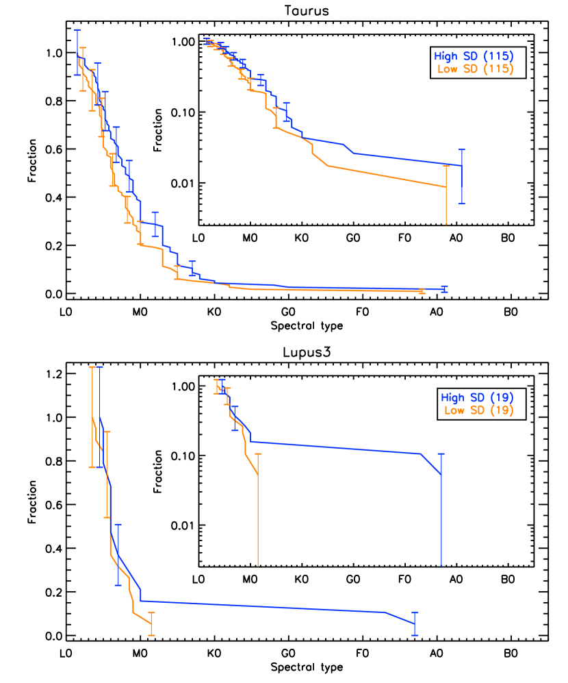
Figure 1.— The fraction of stars with spectral types earlier than each value for stars in the highest (blue) and lowest (orange) third of stellar surface densities, computed using $n=4$. The vertical lines indicate the Poisson error at each spectral type, and the numbers in braces in the legend indicate the total number of stars in each category. The inset plot shows the cumulative number in log space. Stars in Taurus and Lupus3 are shown in this figure.

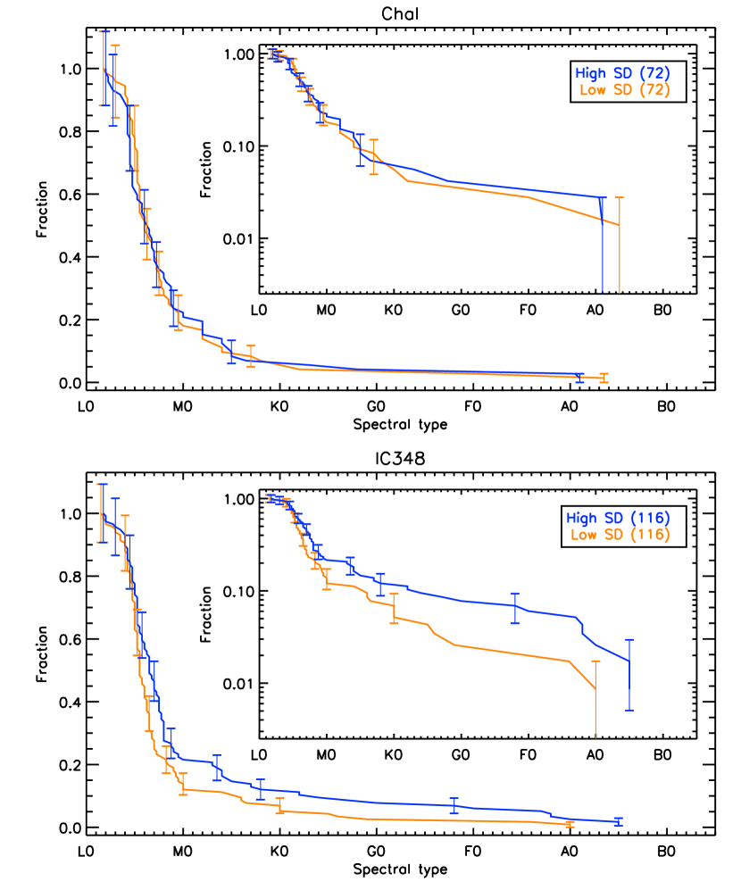
Figure 2.— The distribution of spectral types in the highest and lowest third of source surface densities in ChaI and IC348. See Figure 1 for more details.

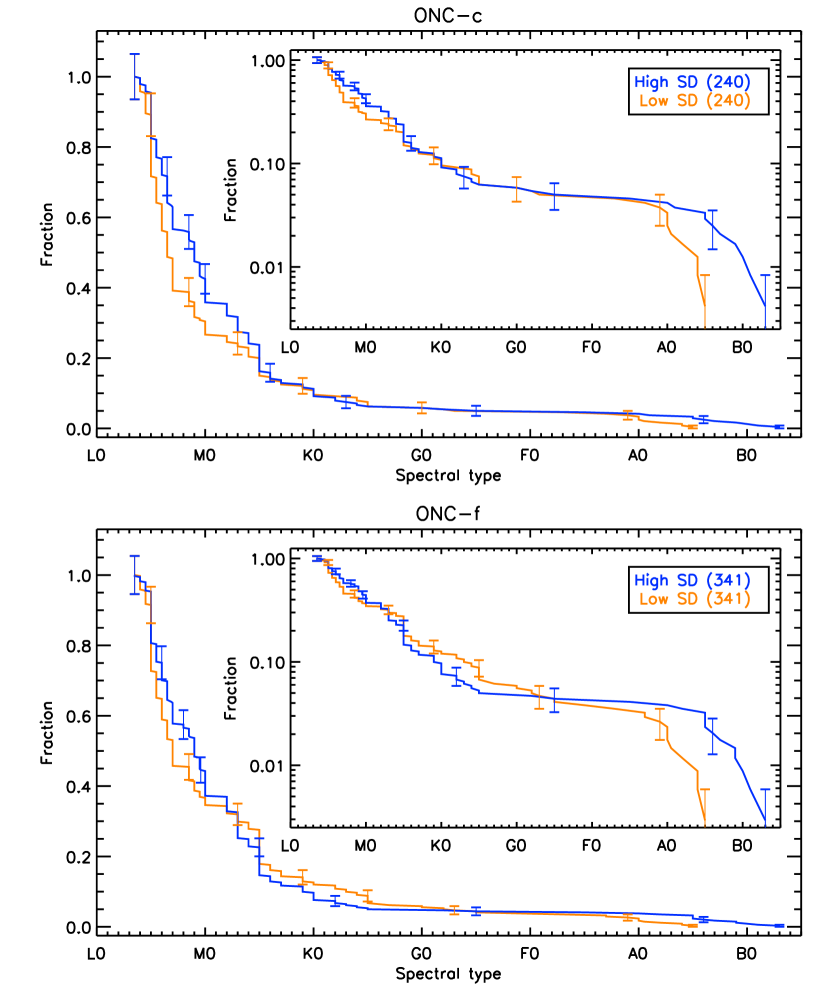
Figure 3.— The distribution of spectral types in the highest and lowest third of source surface densities in the ONC. See Figure 1 for more details.

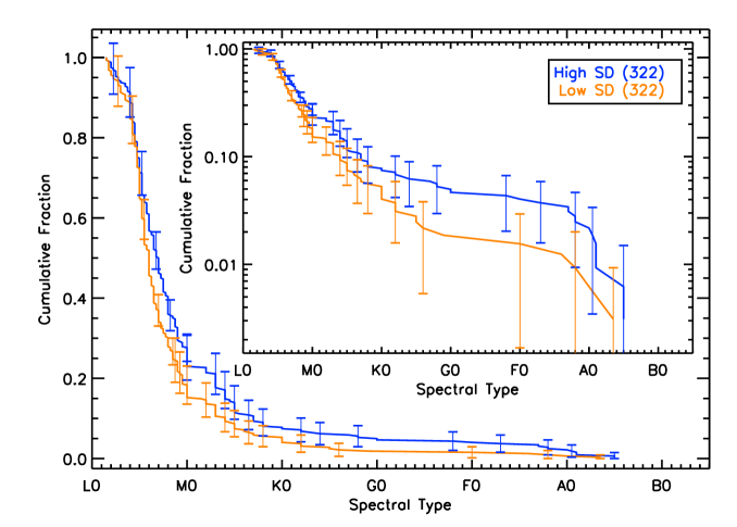
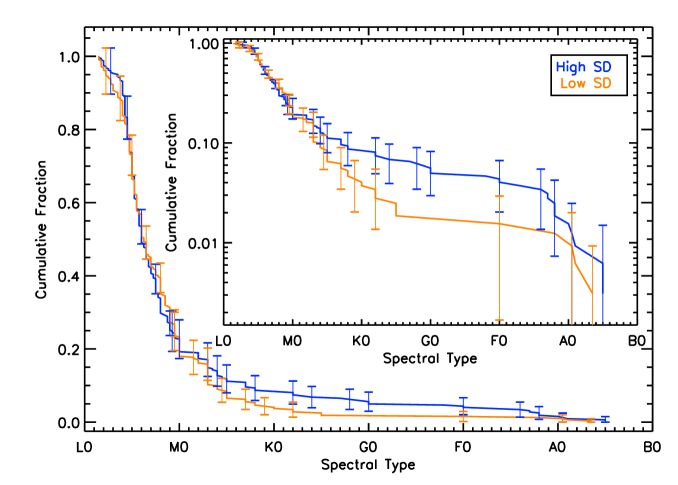
Figure 4.— The distribution of spectral types in the highest and lowest third of surface densities combined over Taurus, Lupus3, ChaI, and IC348. The top panel shows the distributions when combined using the divisions in Figures 1 and 2. The bottom panel shows the distributions when divided using the highest and lowest third of the surface densities compared across all four regions.

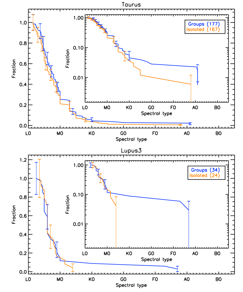
Figure 5.— The distribution of spectral types for grouped and isolated stars. See Figure 1 for the plotting conventions used. Stars in Taurus (top) and Lupus3 (bottom) are shown in this figure.

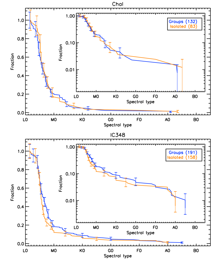
Figure 6.— The distribution of spectral types for grouped and isolated stars. See Figure 1 for the plotting conventions. Stars in ChaI (top) and IC348 (bottom) are shown in this figure.

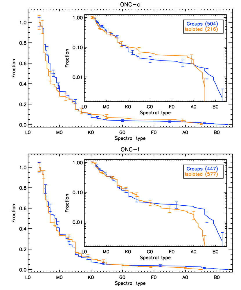
Figure 7.— The distribution of spectral types for grouped and isolated stars. See Figure 1 for the plotting conventions. Stars in the ONC are shown in this figure.

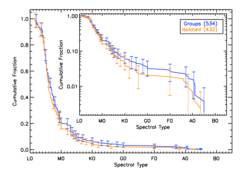
Figure 8.— The distribution of spectral types for grouped and isolated stars summed over all of Taurus, Lupus3, ChaI, and IC348.

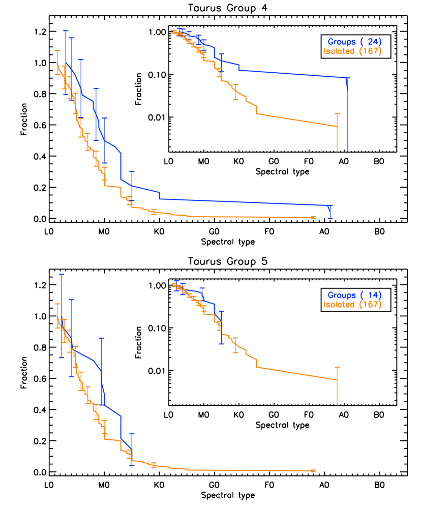
Figure 9.— The distribution of spectral types in the two Taurus groups showing the most significant differences with the isolated populations (based on KS2 and MW statistics). The plot conventions follow those in Figure 1.

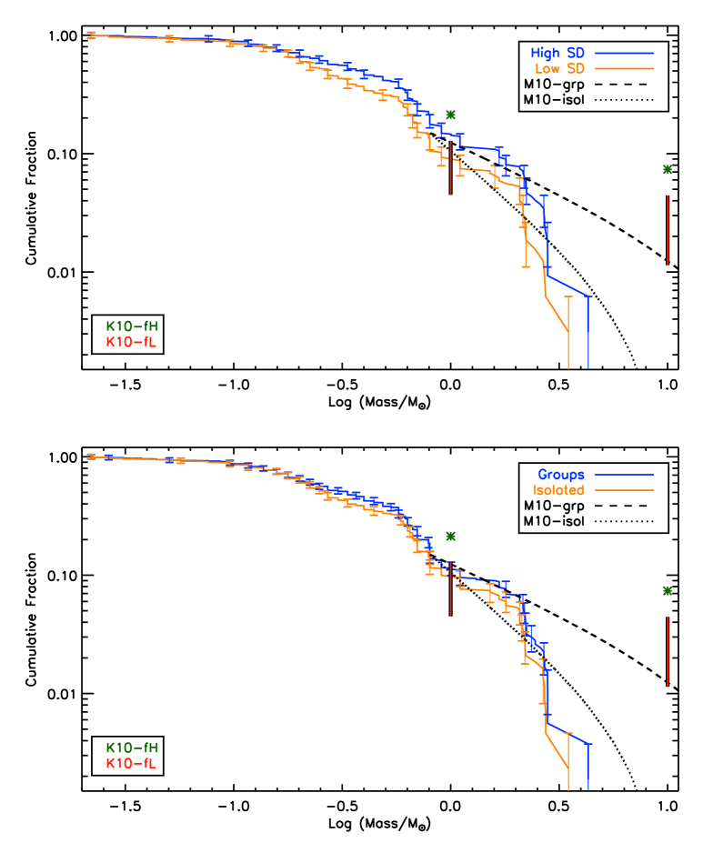
Figure 10.— The cumulative distribution of mass for all four nearby star-forming regions combined. The top panel shows the high and low stellar surface density stars, while the bottom panel shows the grouped and isolated stars. Error bars indicate the Poisson errors. Also shown are predictions from M10 for stars in grouped and isolated environments, scaled to a total fraction of 15% at the lower mass limit of 0.8M_⊙(black dashed and dotted lines respectively). The range of values spanned by the analytic K10 model are shown by the green asterisk (high density model) and red line (range of low density models). The K10 models are not directly comparable to the observations, however, the range spanned by the models should encompass the observations.

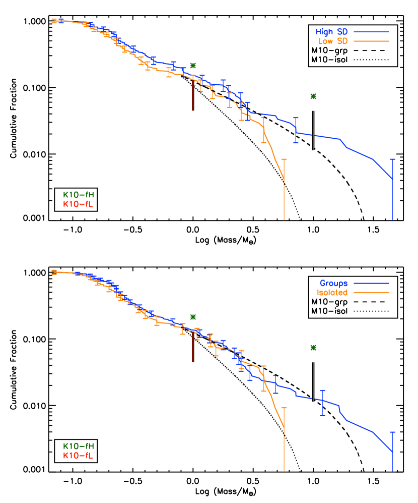
Figure 11.— The cumulative mass distribution for the stars in ONC-c, for the high versus low stellar surface density sources (top panel), and grouped versus isolated sources (bottom panel). Comparisons with predictions by M10 and K10 are shown as in Figure 10; note that the plot ranges differ from the previous figure.

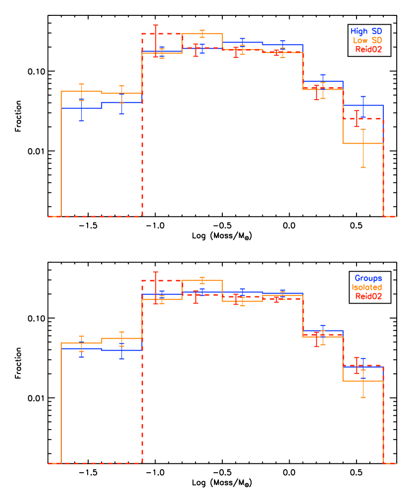
Figure 12.— The differential mass distribution for all four nearby star-forming regions. The top panel shows the high and low stellar surface density stars, while the bottom panel shows the grouped and isolated stars. Error bars indicate Poisson errors. Also shown is the field star mass function measured by Reid et al (2002), corrected for stellar evolution (red line). The errors estimated by Reid et al (2002) are shown offset from the bin centre for clarity.

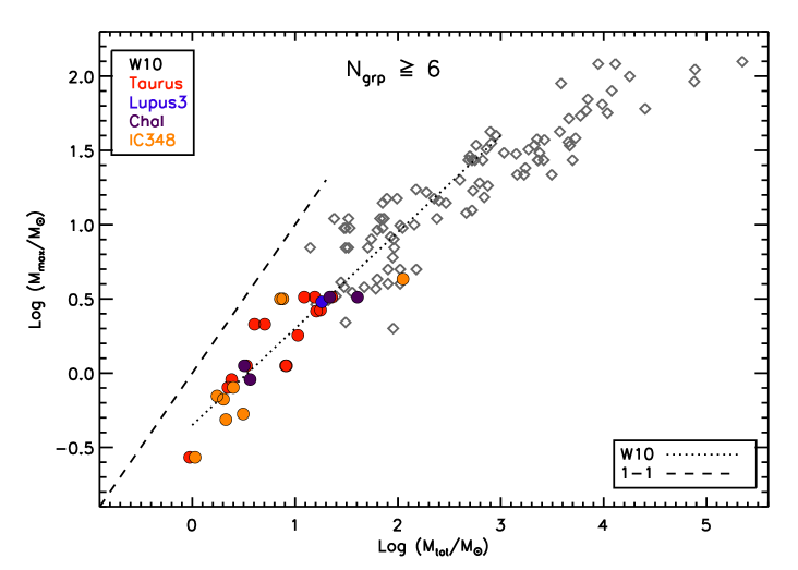
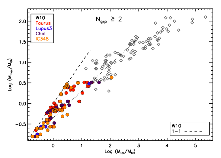
Figure 13.— The mass of the maximum mass member in each stellar grouping versus the total group mass. The data and approximate low-mass slope in Weidner et al (2010) are shown by the grey diamonds and dotted line respectively. The coloured circles show our results for groupings with six or more members (top) and two or more members (bottom). The dashed line shows a 1-1 relationship (the upper limit).

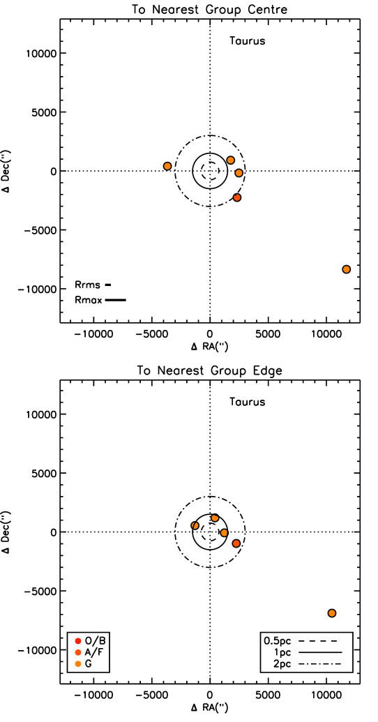
Figure 14.— The separation between each isolated early type star and its nearest group’s centre (top) and the closest group member (bottom) in Taurus. Colours denote different spectral types, and the circles indicate separations of varying amounts. The thick horizontal lines show the mean Rrms and Rmax values for the groups.

References

- Allison et al (2009) Allison, R. J., Goodwin, S. P., Parker, R. J., Portegies Zwart, S. F., de Grijs, R., & Kouwenhoven, M. B. N. 2009, MNRAS, 395, 1449
- Baraffe et al (1998) Baraffe, I., Chabrier, G., Allard, F., & Hauschildt, P. H. 1998, A&A, 337, 403
- Bastian, Covey, & Meyer (2010) Bastian, N., Covey, K. R., & Meyer, M. R. 2010, ARA&A, 48, 339
- Bate, Bonnell, & Bromm (2003) Bate, M. R., Bonnell, I. A., & Bromm, V. 2003, MNRAS, 339, 577
- Bonnell et al. (2003) Bonnell, I. A., Bate, M. R., & Vine, S. G. 2003, MNRAS, 343, 413
- Bonnell et al. (2008) Bonnell, I. A., Clark, P., & Bate, M. R. 2008, MNRAS, 389, 1556
- Bressert et al (2010) Bressert, E., Bastian, N., Gutermuth, R., et al 2010, MNRAS, 409L, 54
- Casertano & Hut (1985) Casertano, S. & Hut, P., 1985 ApJ, 298, 80
- Chabrier et al (2000) Chabrier, G., Baraffe, I., Allard, F., & Hauschildt, P. 2000, ApJ, 542, 464
- Chabrier (2005) Chabrier, G. 2005, in Astrophysics and Space Science Library 327, the Initial Mass Function 50 Years Later, ed. E. Corbelli, F. Palla, & H. Zinnecker (Dordecht: Springer), 41
- Comerón (2008) Comerón, F. 2008, Handbook of Star Forming Regions, Volume II: The Southern Sky, ASP Monograph Publications, Vol. 5, ed. Bo Reipurth, p 295
- Conover (1999) Conover, W. J. 1999, Practical Nonparametric Statistics, 3rd edition. John Wiley & Sons, Inc., New York, pp 271, 456
- Covey et al (2008) Covey, K. R., Hawley, S. L., Bochanski, J. J. et al 2008, ApJ, 136, 1778
- de Wit et al (2004) de Wit, W. J., Testi, L., Palla, F., Vanzi, L., & Zinnecker, H. 2004, A&A, 425, 937
- de Wit et al (2005) de Wit, W. J., Testi, L., Palla, F., & Zinnecker, H. 2005, A&A, 437, 247
- Delgado-Donate, Clarke, &Bate (2003) Delgado-Donate, E. J., Clarke, C. J., & Bate, M. R. 2003, MNRAS, 342, 926
- Goodman & Arce (2004) Goodman, A. A. & Arce, H. G. 2004, ApJ, 608, 831
- Gutermuth et al (2009) Gutermuth, R. A., Megeath, S. T., Myers, P. C. et al 2009, ApJS, 184, 18
- Hillenbrand (1997) Hillenbrand, L. 1997, AJ, 113, 1733
- Hillenbrand & Hartmann (1998) Hillenbrand, L. A. & Hartmann, L. W. 1998, ApJ, 492, 540
- Kharchenko (2001) Kharchenko, N. V. 2001, KFNT, 17, 409
- Kirk & Myers (2011) Kirk, H. & Myers, P. C. 2011, ApJ, 727, 64
- Kiseleva et al (1998) Kiseleva, L. G., Colin, J., Dauphole, B., & Eggleton, P. 1998, MNRAS, 301, 759
- Krumholz & McKee (2008) Krumholz, M. R. & McKee, C. F., Nature, 451, 1082
- Krumholz et al (2010) Krumholz, M. R., Cunningham, A. J., Klein, R. I., & McKee, C. F. 2010, ApJ, 713, 1120
- Lada et al (2006) Lada, C. J., Muench, A. A., Luhman, K. L. et al 2006, AJ, 131, 1574
- Lamb et al (2010) Lamb, J. B., Oey, M. S., Werk, J. K., & Ingleby, L. D. 2010, ApJ, 725, 1886
- Luhman (2007) Luhman, K. L. 2007, ApJS, 173, 104
- Luhman et al (2009) Luhman, K. L., Mamajek, E. E., Allen, P. R., & Cruz, K. L. 2009, ApJ, 703, 399
- Luhman et al (2010) Luhman, K. L., Allen, P. R., Espaillat, C., Hartmann, L., & Calvet, N. 2010, ApJS, 186, 111
- McKee & Tan (2003) McKee, C. F. & Tan, J. C. 2003, ApJ, 585, 850
- Maschberger et al (2010) Maschberger, Th., Clarke, C. J., Bonnell, I. A., & Kroupa, P. 2010, MNRAS, 404, 1061
- Muench et al (2007) Muench, A. A. Lada, C. J., Luhman, K. L., Muzerolle, J., & Young, E. 2007, AJ, 134, 411
- Myers (2009b) Myers, P. C. 2009, ApJ, 706, 1341
- Palla & Stahler (1999) Palla, F. & Stahler, S. 1999, ApJ, 525, 772
- Parker & Goodwin (2007) Parker, R. J. & Goodwin, S. P. 2007, MNRAS, 380, 1271
- Reid et al (2002) Reid, I. N., Gizis, J. E., & Hawley, S. L. 2002, 124, 2721
- Röser et al (2008) Röser, S., Schilbach, E., Schwan, H. et al 2008, A&A, 488, 401
- Röser et al (2010) Röser, S., Demleitner, M., & Schilbach, E. 2010, AJ, 139, 2440
- van Leeuwen (2007) van Leeuwen, F. 2007, A&A, 474, 653
- Vine & Bonnell (2003) Vine, S. G. & Bonnell, I. A. 2003, MNRAS, 342, 314
- Weidner et al (2010) Weidner, C., Kroupa, P., & Bonnell, I. A. D. 2010, MNRAS, 401, 275
- Zacharias et al (2004) Zacharias, N., Monet, D. G., Levine, S. E. et al 2004, AAS, 205, 4815
- Zacharias et al (2010) Zacharias, N., Finch, C., Girard, T. et al 2010, AJ, 139, 2184