WUB/11-16
On the phase structure of five-dimensional SU(2) gauge theories with anisotropic couplings

Abstract

The phase diagram of five-dimensional SU(2) gauge theories is explored using Monte Carlo simulations of the theory discretized on a Euclidean lattice using the Wilson plaquette action and periodic boundary conditions. We simulate anisotropic gauge couplings which correspond to different lattice spacings $a_{4}$ in the four dimensions and $a_{5}$ along the extra dimension. In particular we study the case where $a_{5}>a_{4}$. We identify a line of first order phase transitions which separate the confined from the deconfined phase. We perform simulations in large volume at the bulk phase transition staying in the confined vacuum. The static potential measured in the hyperplanes orthogonal to the extra dimension hint at dimensional reduction. We also locate and analyze second order phase transitions related to breaking of the center along one direction.

1 Introduction

Our interest in studying five-dimensional gauge theories comes from extensions of the Standard Model called Gauge-Higgs unification. The idea is to identify the Higgs boson with (some of) the extra dimensional components of the gauge field. Since five-dimensional gauge theories are non-renormalizable an ultra-violet cut-off is mandatory. The lattice regularization provides such a gauge-invariant cut-off (the inverse lattice spacing) and is therefore a natural setup to study these theories.

Here we consider the five-dimensional pure SU(2) gauge theory and investigate its non-perturbative phase diagram through Monte Carlo simulations. The theory is discretized on a Euclidean space-time lattice. The seminal work done by Creutz [?] using the Wilson plaquette gauge action [?] demonstrated the existence of (at least) two bulk phases in the non-perturbative phase diagram of the theory in infinite volume. There is a confined phase at large values of the gauge coupling and a deconfined phase when the gauge coupling is small.

The question we are after is where dimensional reduction from five to four dimensions occurs. Possible mechanisms, which have been proposed are compactification or localization. In compactification models the size of the extra dimension is small and the system is described by an effective four-dimensional low energy theory valid for energies much below the inverse compactification radius. The existence of a minimal physical size of the extra dimension, below which the theory becomes four-dimensional has been suggested by lattice simulations in [?]. The extra dimension can even “disappear” when the correlation length of the four-dimensional theory grows exponentially fast with the size of the extra dimension. This is the mechanism of D-theory [?,?], which relies on the existence of the Coulomb phase and has been recently studied on the lattice [?].

The most prominent of localization models in flat space is the domain wall construction for fermions [?], which has been shown to be equivalent to an orbifold construction [?]. A possible localization mechanism for gauge field has been proposed in [?] and relies on a mechanism that confines the theory in the bulk and deconfines it on a boundary (or domain wall) of the extra dimension. This mechanism has been studied on the lattice in [?], where it was found that indeed localization occurs but the low energy effective theory contains not just the localized zero-modes but also higher Kaluza–Klein modes. Similarly localization can can also be realized if a layered phase exists [?,?].

The phenomenological signature of extra dimensional models depends on the mechanism of dimensional reduction. In the compactification case a striking evidence would be the appearance of Kaluza–Klein modes. For example, so far the non-observation of an excitation $Z^{\prime}$ of the $Z$ boson at LHC [?,?] has put a lower bound on their mass of about $1\,{\rm TeV}$ (assuming it has the same couplings as the Standard Model particle). This translates into a bound on the inverse compactification radius. In the localization case, there is a spectrum of four-dimensional localized modes at low energies with a mass gap, which is set by the domain wall height $M$ , separating the higher modes. The latter can be localized modes forming like a Kaluza–Klein tower or bulk modes [?,?].

Recently [?,?] the phase diagram of the five-dimensional pure SU(2) gauge theory on the torus discretized with the Wilson plaquette action and anisotropic gauge couplings has been investigated in the mean-field approximation including corrections [?,?]. The mean-field phase diagram exhibits three phases, besides the confined and deconfined phases there is a layered phase when when the lattice spacing along the extra dimension $a_{5}$ is larger than the one in the usual four dimensions $a_{4}$. It is possible to take the continuum limit approaching a critical line (a line of second order phase transitions ) at the phase boundary between the deconfined and the layered phase. The lattice spacings go to zero by keeping the anisotropy and the ratio of the vector to the scalar masses fixed. In this limit the hyperplanes orthogonal to the extra dimension decouple from each other and the theory turns four-dimensional. In the present paper we show what happens when the full theory is simulated by Monte Carlo methods.

The paper starts with Section 2 containing definitions of the lattice theory and observables used in this study. In addition to observables (plaquettes and Polyakov loops and their susceptibilities, Binder cumulants) signaling phase transitions, we compute the static potential in the four-dimensional hyperplanes orthogonal to the extra dimension. Using the latter we define renormalized couplings from the static force and its derivative, which give us information about dimensional reduction. In Section 3 we discuss the case of isotropic couplings (where the lattice spacing is the same in all directions) as a starting point for the investigations of the anisotropic case in Section 4. We study the part of the phase diagram where $a_{5}>a_{4}$. We find first order bulk phase transitions (Section 4.1), which separate the confined from the deconfined phase, and second order phase transitions related to breaking of the center symmetry along one lattice dimension (Section 4.2). In Section 4.3 we show our results for the static potential measured at two bulk phase transition points in the confined vacuum, which hint at dimensional reduction. Our conclusions and outlook are presented in Section 5. Appendix A summarizes the formulae for the 3-loop perturbative running of the coupling derived from the static force in the four-dimensional Yang-Mills theory, which we use to compare with our lattice data.

2 Definitions

We consider a Euclidean lattice in five dimensions. The dimensions are labelled by $M=0,1,2,3,5$. The lattice size is $V=L_{T}\times L_{\rm s}^{3}\times L_{5}$, where $L_{T}$, $L_{\rm s}$ and $L_{5}$ are the number of lattice points in the temporal ($M=0$), spatial ($M=1,2,3$) and extra ($M=5$) dimensions respectively. We use Roman capital letters $M,N,\ldots$ to label all five dimensions and Greek letters $\mu,\nu,\ldots$ to label the four dimensions $0,1,2,3$. The lattice points are denoted by $x=(x_{0},\vec{x},x_{5})$ and the gauge links by $U(x,M)$. The Wilson lattice action for a SU(2) gauge theory is

$$S = \frac{\beta}{2}\sum_{x}\left[\frac{1}{\gamma}\sum_{\mu<\nu}\mathrm{tr}\{1-U(x;\mu,\nu)\}+\gamma\sum_{\mu}\mathrm{tr}\{1-U(x;\mu,5)\}\right]\,,$$ (2.1)

where $U(x;M,N)$ is the oriented plaquette at point $x$ in directions $M$ and $N$ and we use the property that the trace of SU(2) matrices is real. The parameter $\gamma$ is the anisotropy parameter. Instead of $(\beta,\gamma)$ we will also use the equivalent parameter pair

$$\beta_{4}=\frac{\beta}{\gamma}\quad \quad\beta_{5}=\beta\,\gamma\,.$$ , (2.2)

The isotropic lattice corresponds to $\gamma=1$. If $\gamma\neq 1$ there are two different lattice spacings, $a_{4}$ in the $\mu$-dimensions and $a_{5}$ in the extra dimension. At the classical level the relation $\gamma=a_{4}/a_{5}$ holds. The relation between the lattice coupling $\beta$ and the bare dimensionful gauge coupling $g_{5}$ is [?]

$$\beta = \frac{2Na_{4}}{g_{5}^{2}}\,,\;(N=2)\,.$$ (2.3)

The coupling $g_{5}$ is an effective coupling at the cut-off scale and an attempt to define a continuum limit $a_{4}\to 0$ by keeping $g_{5}$ constant (up to a slowly varying renormalization factor) leads to decreasing $\beta$. Eventually the value $\beta_{c}$ at the phase transition between the deconfined and confined phase is reached, meaning that the lattice spacing cannot be further reduced. The continuum limit can therefore only be taken at $g_{5}=0$, i.e. the theory is trivial [?]. Triviality can also be understood by considering the 1-loop renormalization of the effective four-dimensional coupling $g_{4}^{2}=g_{5}^{2}/(L_{5}a_{5})$ [?,?].

In the Monte Carlo simulations of Eq. (2.1) we use the heatbath algorithm proposed by Fabricius and Haan [?] and independently by Kennedy and Pendleton [?] in combination with the overrelaxation algorithm, cf. [?]. One updating unit (or iteration) is typically defined as the sequence of $L_{\rm s}/2$ overrelaxation sweeps followed by one heatbath sweep. In order to check the ergodicity of our simulations we have repeated some of them using Creutz’s version of the heatbath algorithm [?] and a mixture of the Kennedy-Pendleton and Creutz one. The simulation results obtained with these three variants of the algorithm agree very well. The statistical analysis of our simulations is usually done with the method of [?] but in some cases we use the bootstrap method.

The observables that we measure to investigate the phase diagram are the traces of the plaquettes, separately for the plaquettes orthogonal to and along the extra dimension

$${\rm Plaq}_{4}=\frac{1}{6V}\sum_{x}\sum_{\mu<\nu}\mathrm{tr}\{U(x;\mu,\nu)\} {\rm Plaq}_{5}=\frac{1}{4V}\sum_{x}\sum_{\mu}\mathrm{tr}\{U(x;\mu,5)\}\,,$$ ,

and their susceptibilities

$$\chi_{{\rm Plaq}_{i}} = V\left\langle\left({\rm Plaq}_{i}-\left\langle{\rm Plaq}_{i}\right\rangle\right)^{2}\right\rangle\,,\;i=4,5\,.$$ (2.5)

The plaquette observables provide signals for bulk phase transitions. In order to study phase transitions related to the breaking of the center symmetry we also measure Polyakov loops. For example, the Polyakov loop along the time dimension and its susceptibility are defined by

$${\rm Poly}_{T} = \frac{L_{T}}{V}\left|\sum_{\vec{x},x_{5}}\mathrm{tr}\prod_{x_{0}=0}^{(L_{T}-1)a_{4}}U(x,0)\right|$$ (2.6)

$$\chi_{{\rm Poly}_{T}} = \frac{V}{L_{T}}\left\langle\left({\rm Poly}_{T}-\left\langle{\rm Poly}_{T}\right\rangle\right)^{2}\right\rangle\,.$$ (2.7)

Polyakov loops winding in other directions are similarly defined. We will also consider the temporal Polyakov loop without averaging over the extra dimension, explicitely

$${\rm Poly}_{T}(x_{5}) = \frac{1}{L_{\rm s}^{3}}\left|\sum_{\vec{x}}\mathrm{tr}\prod_{x_{0}=0}^{(L_{T}-1)a_{4}}\left.U(x,0)\right|_{x_{5}}\right|$$ (2.8)

$$\chi_{{\rm Poly}_{T}}(x_{5}) = L_{\rm s}^{3}\left\langle\left({\rm Poly}_{T}(x_{5})-\left\langle{\rm Poly}_{T}(x_{5})\right\rangle\right)^{2}\right\rangle\,.$$ (2.9)

It will be clear in the following why we use two different definitions Eq. (2.6) and Eq. (2.8) of the Polyakov loop. Other useful quantities to investigate the order of phase transitions are the Binder cumulants [?]. For example, the fourth order Binder cumulant of the temporal Polyakov loop is

$$B_{4} = 1-\frac{\left\langle{\rm Poly}_{T}^{4}\right\rangle}{3\left\langle{\rm Poly}_{T}^{2}\right\rangle^{2}}\,,$$ (2.10)

and similarly for other quantities.

Wilson loops are traces of product of links along rectangular paths (we consider only on-axis Wilson loops). We measure Wilson loops $W(r,T)$ of size $T$ in the temporal direction and $r$ along one of the spacial dimensions. On anisotropic lattices there are two types of loops, depending whether the distance $r$ is taken along the extra dimension or the other spatial dimensions. In the measurement of the Wilson loops, the temporal links are replaced by their one-link integrals [?] and the spatial links are replaced by the links obtained after two levels of HYP smearing [?]. The HYP smearing of the spatial links is restricted to staples extending in the spatial directions, e.g. for a link in direction $\mu=1$ the staples are in directions $M=2,3,5$. We use the HYP parameters

$$\alpha_{1}=0.8\,, \alpha_{2}=0.56\,, \alpha_{3}=0.24\quad\mbox{(level 1)}\,,$$ (2.11)

$$\alpha_{1}=0.92\,, \alpha_{2}=0.68\,, \alpha_{3}=0.28\quad\mbox{(level 2)}\,,$$ (2.12)

optimized by maximizing the minimum plaquette. We find that these values do not strongly depend on the gauge couplings. We increase the levels of smearing up to four by using for level 3 and 4 the same parameters as for level 2. We checked numerically that the average and minimum plaquette increase with the number of smearing levels since our parameters $\alpha_{1}$ are larger than the perturbative bound on the APE smearing parameter $\alpha\leq 0.75$ [?]. From the Wilson loops we compute the effective masses

$$a_{4}m_{\rm eff}(r,t+a_{4}/2) = \ln\left(\frac{\left\langle W(r,t)\right\rangle}{\left\langle W(r,t+a_{4})\right\rangle}\right)\;\stackrel{{\scriptstyle t\to\infty}}{{\sim}}\;a_{4}V(r)$$ (2.13)

and extract the static potential $V(r)$ from a plateau average of the effective masses at large enough $t$, cf. [?]. In order to determine where to start the plateau average for each value of $r$ we perform a fit

$$m_{\rm eff}(r,t+a_{4}/2) = E+b\,{\rm e}^{-(t+\frac{a_{4}}{2})\Delta}$$ (2.14)

with fit parameters $E$, $b$ and $\Delta$. The plateau average starts at the earliest time $t_{0}$ when the exponential correction in Eq. (2.14) is smaller than 1/4 of the the statistical error of the effective mass. The plateau ends before the time $t$ when either the difference of the effective mass at time $t$ to the one at $t_{0}$ is larger than the error of the effective mass at $t_{0}$ or the error of the effective mass at time $t$ is larger than twice the error of the one at $t_{0}$.

In our analysis we focus on the static potential along spatial directions orthogonal to the extra dimension and we call this potential $V(r)$. We define the static force through the symmetric derivative of the potential

$$F(r-a_{4}/2) = \{V(r)-V(r-a_{4})\}/a_{4}\,.$$ (2.15)

The scale $r_{0}/a_{4}$ [?] is determined through the numerical solution of

$$\left.r^{2}\,F(r)\right|_{r=r_{0}} = 1.65\,,$$ (2.16)

which we find using a 2-point interpolation of the force $F(r)=f_{0}+f_{2}/r^{2}$. A comparison with a 3-point interpolation adding a $f_{4}/r^{4}$ term allows to estimate the systematic error. From the static force, a running coupling can be defined (in the so called qq-scheme)

$$\alpha_{\rm qq}(1/r) = \frac{1}{C_{\rm F}}\,r^{2}\,F(r)\,,$$ (2.17)

where $C_{\rm F}=3/4$ for gauge group SU(2). The perturbative expansion up to three loops of $\alpha_{\rm qq}$ in four-dimensional Yang–Mills theory is summarized in Appendix A. By taking a further derivative we compute the slope [?]

$$c(r) = \frac{1}{2}\,r^{3}\,F^{\prime}(r)\,,$$ (2.18)

which also defines a running coupling (at small distances). On the lattice we compute $c(r)$ through

$$c(r) = \frac{1}{2}\,r^{3}\,\{V(r+a_{4})+V(r-a_{4})-2V(r)\}/a_{4}^{2}\,.$$ (2.19)

At large distances, the slope can be compared to the result of effective bosonic string theory [?,?], which yields the asymptotic value

$$c(\infty) = -\frac{(D-2)\pi}{24}\,,$$ (2.20)

where $D$ is the number of space-time dimensions. Thus $c$ can serve to determine the number of dimensions. We remark that due to the factor $r^{3}$ in its definition, the noise-to-signal ratio of $c(r)$ rapidly deteriorates when $r$ grows.

Since most of our large volume simulations are done at $\gamma<1$ in the confined phase, it turns out that the static potential along the extra dimension $V_{5}(r)$ is difficult to extract. The reason is that the values of $a_{4}V_{5}(r)$ we measure at $r=2a_{5}$ are typically 1 or larger and the dimensionless string tension (the coefficient of the term in $V_{5}(r)$ which is linear in $r$) $a_{4}a_{5}\sigma_{5}$ contains the large lattice spacing $a_{5}$.

3 Isotropic couplings

The aim of this section is to review known results for and highlight features of the isotropic case ($\gamma=1$) that will be of help in the understanding of the anisotropic ($\gamma\neq 1$) case. We will start with the description of the system at zero temperature in the “infinite” volume limit. Afterwards we will analyze how any kind of finite size affects the results.

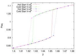
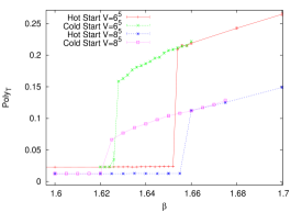
Figure 1: Plaquette and Polyakov expectation value as function of $\beta$ on isotropic lattices.

The phase diagram of the five-dimensional isotropic SU(2) lattice gauge theory is well known since the early work of Creutz [?]. In the zero temperature setting and at infinite volume (both spatial and in the extra-dimension) the phase diagram of the model is characterized by the presence of a bulk first order phase transition at a critical value of the lattice coupling $\beta=\beta_{c}\approx 1.64$. The bulk phase transition is characterized by the appearance of a strong hysteresis region in the expectation value of the plaquette, see Fig. 1, that survives in the infinite volume limit, signal of the presence of latent heat at the transition point. The two regions separated by $\beta_{c}$ have a different behavior of the Wilson loop, with a string tension (the coefficient $\sigma$ of the linear term $\sigma\,r$ in the static potential $V(r)$) different from zero in the confined phase for $\beta<\beta_{c}$ and a string tension equal to zero in the deconfined phase above $\beta_{c}$. On a finite (but large) lattice this coincides with a distribution of the Polyakov loop (for all directions and not taking the absolute value) being always peaked in zero in the first case, while always showing a double peak structure in the second case.

In Fig. 1 we report an example of the typical plots showing the behavior at the phase transition both for the expectation value of the plaquette and of the absolute value of the temporal Polyakov loop ${\rm Poly}_{T}$ defined in Eq. (2.6). “Hot Start” or “Cold Start” means that the simulation starts from an initial configuration with random gauge links or gauge links set to the identity, respectively. We perform $10^{4}$ measurements separated by 10 updating iterations.

3.1 One “small” dimension

Now we investigate the effects of the finite lattice size on our observables and how they affect the bulk phase transition. As it is well known there is no sign of first order bulk phase transition in four-dimensional SU(2) Yang–Mills theory, instead a sharp crossover separates the weak and the strong coupling regime. It is then legitimate to ask which is the fate of the five-dimensional bulk phase transition when we consider the five-dimensional system compactified along one “small” direction.

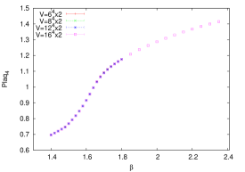
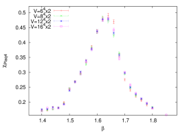
Figure 2: Expectation values of the plaquette ${\rm Plaq}_{4}$ and its susceptibility $\chi_{{\rm Plaq}_{4}}$ as function of $\beta$ on lattices with $L_{5}=2$ and different values of $L_{T}=L_{\rm s}=6,\ldots,16$.

If we consider a geometry that has one small direction while all the other directions are sent to infinity, namely $L_{5}\ll L_{T}=L_{\rm s}$, we notice that the bulk phase transition at $\beta=1.64$ “evaporates” and lets a smooth cross-over appear, cf. the early work of [?]. This is shown by the behavior of the four-dimensional plaquette ${\rm Plaq}_{4}$ Eq. (LABEL:plaqs) and of its susceptibility $\chi_{{\rm Plaq}_{4}}$ Eq. (2.5) in Fig. 2, for $L_{5}=2$ and different choices of the four-dimensional lattice size $L_{T}=L_{\rm s}=6,\ldots,16$. There is no dependence nor on the initial condition (hot or cold start) of the simulation neither on the lattice volume. The cross-over region is close to $\beta=1.48$ and will be investigated below. The susceptibility of the plaquette shows a peak at $\beta$ values reminiscent of the bulk phase transition but whose magnitude is independent on the volume. We extend the simulations for our largest $2\times 16^{4}$ lattice up to $\beta=2.4$ but we do not see any sign of the cross-over of the four-dimensional SU(2) theory, which is at $\beta\approx 2.3$ [?].

Our simulations hint at the existence of a minimal lattice size

$$2<L^{\rm min}(\gamma=1)<6\,,$$ (3.21)

for which if one or more of the lattice dimensions are smaller then $L^{\rm min}(\gamma=1)$ we are unable to detect any sign of the bulk phase transition.

Volume	$\beta_{c}$ (${\rm Poly}_{T}$)	$\beta_{c}$ (${\rm Poly}_{T}(1)$)	$\chi_{c}$ (${\rm Poly}_{T}$)	$\chi_{c}$ (${\rm Poly}_{T}(1)$)
$2\times 4^{4}$	1.50061(19)	1.50369(23)	11.86(4)	3.842(15)
$2\times 6^{4}$	1.49097(13)	1.49249(14)	30.00(13)	6.571(19)
$2\times 8^{4}$	1.48748(11)	1.48839(10)	56.9(4)	9.44(5)
$2\times 10^{4}$	1.48570(10)	1.48621(12)	93.1(8)	12.19(9)
$2\times 16^{4}$	1.483952(16)	1.484170(18)	257.8(1.6)	20.88(10)
$2\times\infty^{4}$	1.48280(1)	1.48280(3)	-	-

Table 1: For the center breaking phase transition at $\gamma=1$, $L_{T}=2$, we list the critical values of the coupling $\beta_{c}$ and the susceptibility of the temporal Polyakov loop $\chi_{c}$ as function of the volume. We use two definitions of the Polyakov line, Eq. (2.6) and Eq. (2.8).

Apart from the study of the plaquette, other interesting signals come from the study of the expectation value of the Polyakov loops and their susceptibility in the geometry with one small direction. It is interesting to notice that together with the disappearance of the bulk phase transition also the double peak structure of the Polyakov line distribution along the large directions disappears. On the other side we expect, and find, a proper center breaking structure along the small direction, which we choose for this study to be the temporal one. In order to avoid the appearance of the bulk phase transition we always request that $L_{T}<L^{\rm min}(\gamma=1)$. Notwithstanding the fact that we need to fix $L_{T}$ to a finite value, we can send the orthogonal space size $L=L_{\rm s}=L_{5}$ to infinity and obtain a system that undergoes a proper phase transition. We performed a study of the finite size scaling properties of this breaking by investigating both the distribution of the temporal Polyakov loop and its Binder cumulant (as discussed in [?]) as function of the orthogonal lattice size, while keeping $L_{T}=2$ fixed.

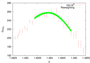
Figure 3: The susceptibility of ${\rm Poly}_{T}$ for the volume $2\times 16^{4}$. Comparison of the directly simulated data set (plusses) and the reweighted data (crosses).

We did a scan in $\beta$ for the different choices of the lattice volume and we used a reweighting technique to obtain a more dense scan. The technique is the multi-histogram reweighting method [?]. Its main idea is to find iteratively the free energy of the system as function of the couplings using all the simulations performed in the region of interest. Once the procedure has converged, we have access via the free energy to all the physical quantities that can be normally extracted in a Monte Carlo simulation, for each value of the coupling constants in the region. Our implementation is able to handle simultaneous reweighting in both the couplings $\beta_{4}$ and $\beta_{5}$, even though in this section we are interested in the $\beta_{4}=\beta_{5}$ case.

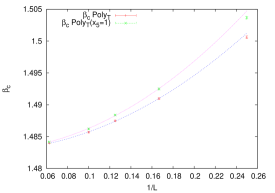
Figure 4: Finite size scaling analysis for the transition at $\gamma=1$, $L_{T}=2$ based on Table 1. We use two definitions of the temporal Polyakov loop, Eq. (2.6) (plusses) and Eq. (2.8) (crosses). The lines are fits to the data using the critical exponents of the four-dimensional Ising model.

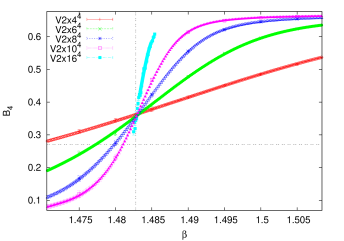
Figure 5: Finite size scaling analysis for the transition at $\gamma=1$, $L_{T}=2$: the Binder cumulant $B_{4}$ of ${\rm Poly}_{T}$ as a function of $\beta$ for several values of $L=L_{\rm s}=L_{5}$.

In order to determine the error of our estimates we use the bootstrap method and do a reweighting analysis over each bootstrap sample. The underlying idea is to consider the estimates coming from each bootstrap sample as independent measurements and to use the spread of these measurements to define the error of the average of the estimates. In Fig. 3 we clearly see that our reweighted estimates for the susceptibility $\chi_{{\rm Poly}_{T}}$ (crosses, they appear like a band in the figure) Eq. (2.7) are more precise than the measurements themselves (plusses). This is however not surprising, since the reweighting technique uses for each estimate the statistical information coming from all the simulated points.

The critical coupling $\beta_{c}$ is defined as the coupling at which the susceptibility $\chi_{{\rm Poly}_{T}}$ has its maximum $\chi_{c}\equiv\chi_{{\rm Poly}_{T}}(\beta_{c})$. The results for $\beta_{c}(L)$ and $\chi_{c}(L)$ as a function of the lattice size $L=L_{\rm s}=L_{5}$ are listed in Table 1. We plot them in Fig. 4, where the plusses refer to the Polyakov line averaged along the extra dimension, Eq. (2.6) and Eq. (2.7), and the crosses refer to the Polyakov line evaluated in the first slice along the extra dimension, Eq. (2.8) and Eq. (2.9). In order to define the error of the derived observables $\beta_{c}(L)$ and $\chi_{c}(L)$ at the critical point we used again the bootstrap procedure. We studied both the bootstrap analysis of the reweighted susceptibility and the distribution of the critical value fitted on each bootstrap sample. The first analysis is used only to define a fitting range for the second one. The critical behavior of a second order phase transition is

$$\chi_{c}(L)\,\equiv\,\chi_{{\rm Poly}_{T}}(\beta_{c}(L)) \sim L^{\gamma/\nu}\,,$$ (3.22)

$$|\beta_{c}(L)-\beta_{c}(L=\infty)| \sim L^{-1/\nu}\,.$$ (3.23)

We do not have enough data to predict in a reliable way the critical exponents. But what we can clearly state is that all our predictions are totally compatible with a phase transition of second order and the scaling behavior dictated by the critical exponents of the four-dimensional Ising model, where $\gamma$ and $\nu$ are respectively $1$ and $1/2$, as expected from [?]. The lines in Fig. 4 are fits to our data using the critical exponent of the four-dimensional Ising model. For $\beta_{c}$ we fit the data for $L>4$ and the fits work well. For $\chi_{c}$ we fit $L>6$ but there are still some non-scaling features which means that we would need bigger volumes. We estimate $\beta_{c}(L=\infty)=1.48280(1)$. There is perfect agreement between the determination of $\beta_{c}$ using both definitions of ${\rm Poly}_{T}$, see Table 1. We emphasize that the two definitions of the Polyakov line must (and indeed they do) lead to the same value for the critical coupling in infinite volume and the same value for the critical exponents. We notice that the deviations from scaling are larger for the definition without the average along the extra dimension and the autocorrelation times are bigger but still under control.

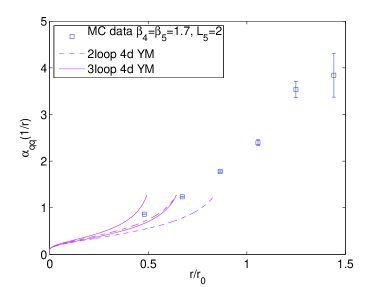
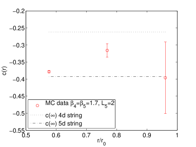
Figure 6: The coupling $\alpha_{\rm qq}$ and the slope $c$ on a isotropic lattice with $L_{5}=2$ at $\beta=1.7$.

In Fig. 5 we show the Binder cumulant $B_{4}$ of the temporal Polyakov loop Eq. (2.10) (here we use only the definition of ${\rm Poly}_{T}$ in Eq. (2.6)). We plot the directly simulated (symbols in the legend) and the reweighted data together. The Binder cumulants tend to intersect at the value $\beta_{c}(L=\infty)$ marked by a vertical line. Looking at Fig. 5 on the right hand side of the intersection “point” the smallest volume ($L=4$) corresponds to the lowermost data points and the largest volume ($L=16$) to the uppermost data points. The value of the intersection is for our small lattice sizes $L$ still far from the analytic estimate for the universality class of the four-dimensional Ising model $B_{4}^{c}\approx 0.27$ (horizontal line in Fig. 5) [?], indicating again that larger values of $L$ would be necessary for a complete analysis. As discussed in [?] the values of $B_{4}$ computed at $\beta_{c}(L=\infty)$ approach $B_{4}^{c}$ with corrections which slowly decrease like $1/\ln(L)$. For our volumes an extrapolation of $B_{4}$ at $L=\infty$ is not feasible. Our strongest evidence for the universality class of the four-dimensional Ising model comes from the scaling analysis presented in Fig. 4.

We have computed the static potential $V(r)$ on $32^{4}\times 2$ lattices at $\beta=1.7$. We ran 4 replica for a total of $4\times 10^{4}$ measurements. Each replicum used 64 cores of the supercomputer Cheops of the University of Cologne and consists of $10^{4}$ update iterations (each iteration does one heatbath and 16 overrelaxation sweeps) for thermalization and $10^{4}$ measurements of the Wilson loops separated by 10 update iterations. We take two levels of HYP smearing for the spatial links of the Wilson loops. We measure the potential starting from distance $r=2a$ and the force from $r=2.5a$. For the fit of the effective masses in Eq. (2.14) we use the range $t=2,3,\ldots,6$. We obtain the scale $r_{0}/a=5.21(7)$ with an integrated autocorrelation time $\tau_{\rm int}(r_{0})=0.5$. The potential can be fitted for $r>r_{0}$ by the form predicted from the effective bosonic string theory and we estimate the string tension to be $\sigma\,r_{0}^{2}=1.6(3)$. The left plot in Fig. 6 shows our data for the coupling $\alpha_{\rm qq}(1/r)$ defined in Eq. (2.17) as a function of $r/r_{0}$. For comparison we plot the 2-loop (dashed) and 3-loop (solid) perturbative curves for the SU(2) Yang–Mills theory in four dimensions, as explained in Appendix A. The data at our smallest distance agree with the 3-loop perturbative curve. The results for the slope $c(r)$ defined in Eq. (2.18) are shown in the right plot of Fig. 6. There is a trend towards the value $c(\infty)=-\pi/12$ predicted by the effective bosonic string in four dimension (marked by the dotted line), but the statistical errors are already too large at distance $r=r_{0}$.

4 Anisotropic couplings

In order to outline the phase diagram of the system at $\gamma\neq 1$ we start from the already known results for $\gamma=1$ and follow the evolution of the various “critical points” as function of $\beta_{4}$ and $\beta_{5}$ for the different lattice geometries that we presented. The critical lines can be cataloged in the following groups:

• bulk phase transitions.
  This kind of transition seems to be always present if the geometry of the lattice is large enough, i.e. in the “infinite volume” and zero temperature limit. More precisely for any fixed $\gamma$ we find a window of values of $\beta_{4}$ and $\beta_{5}$ in which we detect a bulk phase transition signaled by an hysteresis effect in the quantities ${\rm Plaq}_{4}$ and ${\rm Plaq}_{5}$. The hysteresis is seen provided the volume is large enough:

  $$L_{5}>L^{\rm min}_{5}(\gamma) \min\{L_{\rm s}\,,\,L_{T}\}>L^{\rm min}_{\rm s}(\gamma)\,.$$ and (4.24)

• Center breaking phase transitions in the temporal direction (or analogously in any other space direction other than the extra dimension).
  This kind of transition can be obtained by considering a small temporal direction $L_{T}<L^{\rm min}_{\rm s}(\gamma)$ and the other directions larger than their respective minimal sizes. The order parameter is the Polyakov loop ${\rm Poly}_{T}$.

• Center breaking phase transitions in the extra direction.
  This kind of transition is obtained with a small extra dimension $L_{5}<L^{\rm min}_{5}(\gamma)$ while the other dimensions are larger than $L^{\rm min}_{\rm s}(\gamma)$. The order parameter is the Polyakov loop winding along the $M=5$ direction.

4.1 Bulk phase transitions

$\beta_{4c}$	$\beta_{5c}$	$L_{\rm s}$	$r_{0}/a_{4}$
1.865	1.34	10
1.955	1.24	10
2.33	0.937	14	4.774(44)
2.5	0.8697	20	8.46(11)

Table 2: Critical couplings for the bulk phase transition and estimates $L_{\rm s}$ for the minimal lattice size $L^{\rm min}_{\rm s}$ required to be in large four-dimensional volume and see the first order transition. Where we determined it, we list the values of the scale $r_{0}/a_{4}$.

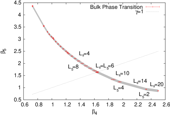
Figure 7: Bulk phase transitions (plusses, the grey band is to guide the eye) of the five-dimensional SU(2) gauge theory using the anisotropic Wilson plaquette action. We indicate estimates $L_{\rm s}$ and $L_{5}$ for the minimal values $L^{\rm min}_{\rm s}$ and $L^{\rm min}_{5}$, see Eq. (4.24), required to see that the transitions in this plot are first order.

Fig. 7 shows the behavior of the bulk phase transition in the $(\beta_{4},\beta_{5})$ parameter plane. The points (plusses) have been determined by simulations and their “errors” are the width of the hysteresis on the largest lattices we have simulated and are therefore only indicative. The phase transition is everywhere first order and we draw a grey band through the points to guide the eye. We put values for $L_{\rm s}$ (that are valid also for $L_{T}$) and $L_{5}$ which are sufficiently large to see the hysteresis signal in the plaquettes and are therefore our estimates for the minimal sizes $L^{\rm min}_{\rm s}$ and $L^{\rm min}_{5}$. The dotted line simply represents the couplings corresponding to $\gamma=1$.

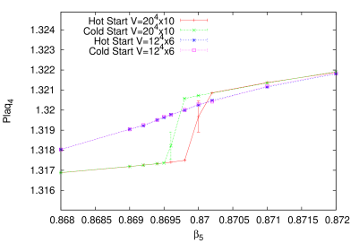
Figure 8: Scan in $\beta_{5}$ of the plaquette ${\rm Plaq}_{4}$ at $\beta_{4}=2.5$. Lattices with $L_{s}$ and $L_{T}$ equal to 20 or larger are needed to see the hysteresis.

In [?] it was claimed that at $\beta_{4}=3.0$ and $\beta_{5}=0.779(1)$ the bulk phase transition turns second order, as it was found in a mean-field computation [?,?]. At $\beta_{4}=3.0$ lattices of much larger size than the ones simulated so far are needed in order to determine the order of the phase transition. Given the large computational effort, at present we cannot comment on the situation at $\beta_{4}=3.0$. In Fig. 8 we present our results at $\beta_{4}=2.5$. We show the behavior of ${\rm Plaq}_{4}$ as a function of $\beta_{5}$ for simulations with a hot start or a cold start. Each simulation consists of $10^{4}$ measurements separated by 10 update iterations, composed by 1 heatbath and $L_{\rm s}/2$ overrelaxation sweeps each. We keep $L_{T}=L_{\rm s}$ and $L_{5}=L_{\rm s}/2$. Fig. 8 shows that for $L_{\rm s}=12$ (asterisks for the hot and empty squares for the cold run) there is no hysteresis but a smooth cross-over. For $L_{\rm s}=20$ (plusses for the hot and crosses for the cold run) the hysteresis appears indicating the presence of a bulk first order phase transition. We list some values of the critical couplings for the bulk phase transition at $\gamma<1$ in Table 2. These couplings are chosen to be approximately in the middle of the hysteresis region. Table 2 also contains the lattice size $L_{\rm s}$ which is sufficiently large to see the hysteresis and is our estimate of $L^{\rm min}_{\rm s}$ in Eq. (4.24). If $L_{T}$ or $L_{\rm s}$ is chosen smaller than $L^{\rm min}_{\rm s}$ one sees a cross-over which is due to “compactification” of the temporal or spatial dimension respectively.

4.2 Center breaking phase transitions

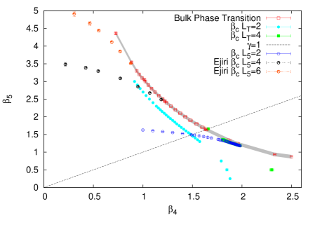
Figure 9: The phase diagram of the five-dimensional SU(2) gauge theory with the anisotropic Wilson plaquette action. Explanations are in the text.

In Fig. 9 we complete our phase diagram of five-dimensional SU(2) gauge theories in the $(\beta_{4},\beta_{5})$ coupling plane of the anisotropic Wilson plaquette gauge action. In addition to the first order bulk phase transitions (empty squares), studied in Section 4.1, we plot phase transitions due to center breaking (or compactification) along either the temporal or the fifth dimension. The order parameter is the Polyakov loop in the temporal or fifth dimension respectively. Our new results are mainly at $\gamma<1$ (i.e. $\beta_{4}>\beta_{5}$, the region below the dashed line in Fig. 9). For $\gamma>1$ (i.e. $\beta_{4}<\beta_{5}$, the region above the dashed line in Fig. 9) we include the points of [?]. In [?,?,?] the transitions due to compactification of the fifth dimension have been studied and found to be second order. These transitions are represented by empty circles in Fig. 9. For $L_{5}=2$ they extend the $\gamma=1$ transition which we discussed in Section 3. This line ends at $\gamma<1$ around $\beta_{4}=2$ when it “hits” the bulk phase transition line. The transitions at $L_{5}=4$ and $L_{5}=6$ found in [?] branch off the bulk phase transition line at $\gamma>1$ as $\beta_{4}$ is lowered more and more.

Volume	$\beta_{4c}$ (${\rm Poly}_{T}$)	$\beta_{4c}$ (${\rm Poly}_{T}(1)$)	$\chi_{c}$ (${\rm Poly}_{T}$)	$\chi_{c}$ (${\rm Poly}_{T}(1)$)
$2\times 8^{3}\times 4$	1.83535(14)	1.83751(25)	46.38(18)	16.69(7)
$2\times 12^{3}\times 6$	1.82713(19)	1.82859(20)	112.6(1.4)	29.3(3)
$2\times 16^{3}\times 8$	1.82455(20)	1.82588(19)	216(5)	44.4(9)
$2\times 20^{3}\times 10$	1.82325(7)	1.82393(8)	351(5)	57.4(6)
$2\times 24^{3}\times 12$	1.82263(3)	1.82309(4)	525(6)	70.9(5)
$2\times\infty^{4}$	1.82115(8)	1.82095(19)	-	-

Table 3: For the center breaking phase transition at $\beta_{5}=0.5$, $L_{T}=2$, we list the critical values of the coupling $\beta_{4c}$ and the susceptibility of the temporal Polyakov loop $\chi_{c}$ as function of the volume. We use two definitions of the Polyakov line, Eq. (2.6) and Eq. (2.8).

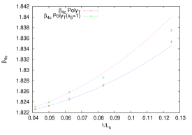
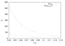
Figure 10: Finite size scaling analysis for the transition at $\beta_{5}=0.5$, $L_{T}=2$ based on Table 3. We use two definitions of the temporal Polyakov loop, Eq. (2.6) (plusses) and Eq. (2.8) (crosses). The lines are fits to the data using the critical exponents of the four-dimensional Ising model.

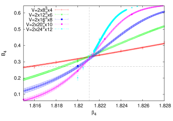
Figure 11: Finite size scaling analysis for the transition at $\beta_{5}=0.5$, $L_{T}=2$: the Binder cumulant $B_{4}$ of ${\rm Poly}_{T}$ as a function of $\beta_{4}$ for several volumes.

In this article we study the transitions due to compactification of the temporal dimension. For $L_{T}=2$ (filled circles in Fig. 9) they are again continuation of the $\gamma=1$ transition. We performed a finite size scaling analysis for the transition point at $\beta_{5}=0.5$. In Table 3 we list the critical values $\beta_{4c}$ of the coupling $\beta_{4}$ at which the susceptibility of the temporal Polyakov line has its maximum $\chi_{c}$ for several values of the lattice size $L_{\rm s}=8\ldots 24$ keeping $L_{5}=L_{\rm s}/2$. We use both definitions of the Polyakov line averaged along the extra dimension Eq. (2.6) or taken on a fixed slice $x_{5}=1$ Eq. (2.8). In Fig. 10 we plot the data as function of $1/L_{\rm s}$ together with fits using the critical exponents of the four-dimensional Ising model, cf. Eq. (3.22) and Eq. (3.23) with $\beta_{c}$ replaced by $\beta_{4c}$ and $L$ by $L_{\rm s}$. The fits work quite well and using the largest three volumes we estimate the critical value $\beta_{4c}(L_{\rm s}=\infty)=1.82115(8)$. Both definitions of the Polyakov line give a perfectly compatible result.

In Fig. 11 we show the results for the Binder cumulant $B_{4}$ of the temporal Polyakov loop Eq. (2.10) (here we use only the definition of ${\rm Poly}_{T}$ in Eq. (2.6)). We apply the reweighting technique as discussed in Section 3 to get a denser data set. There is clear trend in the data to intersect at a common value. The vertical line marks $\beta_{4c}$ and the horizontal line the expected value for the universality class of the four-dimensional Ising model [?]. In order to precisely determine the critical behavior larger volumes are needed. Please note that the lattices which we simulated already require significant computational resources.

Volume	$\beta_{4c}$ (${\rm Poly}_{T}(1)$)	$\chi_{c}$ (${\rm Poly}_{T}(1)$)
$4\times 12^{3}\times 6$	2.3024(8)	23.44(16)
$4\times 16^{3}\times 8$	2.2993(5)	41.1(3)
$4\times 20^{3}\times 10$	2.2995(6)	62.2(5)
$4\times 24^{3}\times 12$	2.2985(10)	88(3)
$4\times 32^{3}\times 16$	2.2981(4)	156(2)
$4\times\infty^{4}$	2.2974(4)	-

Table 4: For the center breaking phase transition at $\beta_{5}=0.5$, $L_{T}=4$, we list the critical values of the coupling $\beta_{4c}$ and the susceptibility of the temporal Polyakov loop $\chi_{c}$ as function of the volume. We only use the definition of the Polyakov line Eq. (2.8).

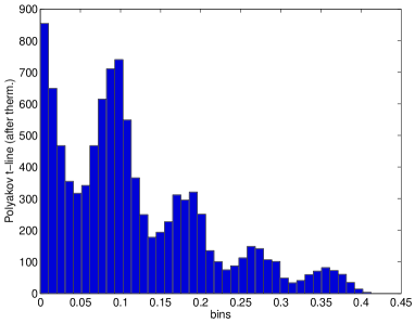
Figure 12: Histograms of the absolute value of the temporal Polyakov loop at $\beta_{4}=2.32$, $\beta_{5}=0.5$ and $L_{T}=4$: taking the definition Eq. (2.6) (average over the extra dimension, left plot) or Eq. (2.8) (at a fixed slice $x_{5}=1$, right plot).

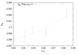
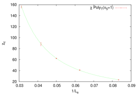
Figure 13: Finite size scaling analysis for the transition at $\beta_{5}=0.5$, $L_{T}=4$ based on Table 4. The temporal Polyakov line is taken in the slice $x_{5}=1$. The lines are fits to the data using the critical exponents of the four-dimensional Ising model.

For $L_{T}=4$ (filled squares in Fig. 9) we faced a new situation. Staying at $\beta_{5}=0.5$ (like for $L_{T}=2$), in the broken phase close to the phase transition the histogram of the temporal Polyakov loop Eq. (2.6) shows several peaks. This is shown by the plot on the left of Fig. 12 for $\beta_{4}=2.32$. If we do not average the Polyakov loop along the fifth dimension and take its definition Eq. (2.8) for the slice $x_{5}=1$, we get the histogram shown by the plot on the right of Fig. 12. There is only a single peak. The interpretation of these plots is that we are in a phase of the theory where the Polyakov lines can fluctuate almost independently in the hyperplanes orthogonal to the fifth dimension. In each hyperplane the distribution of their values has the characteristic double-peak shape which appears like the plot on the right of Fig. 12 when taking the absolute value. When averaging over the hyperplanes they produce a multiple-peak structure, which is therefore an artefact and does not mean the presence of multiple (more than two) vacua. This is a very interesting effect signaling that the interactions between the hyperplanes is weak. The decoupling of the hyperplanes for $\gamma<1$ was in fact also found by the mean-field computation of [?]. While the geometrical setup of our computation is different, the qualitative feature we see are the same.

Taking the temporal Polyakov line defined only on the slice $x_{5}=1$ we can do a finite size scaling analysis as we previously did for $L_{T}=2$. It is now clear why we defined two Polyakov loop operators. Indeed in the present case only for the one not averaged over the extra dimension a finite size scaling analysis can be made. Where it was possible to perform both analyses, we showed that their results coincided. The critical values $\beta_{4c}$ and the maximum of the susceptibility $\chi_{c}$ are listed in Table 4 and shown in Fig. 13. The fits to the critical behavior Eq. (3.22) and Eq. (3.23) assuming the critical exponents of the four-dimensional Ising model work well and give $\beta_{4c}(L_{\rm s}=\infty)=2.2974(4)$.

In summary the phase transitions due to compactification of the temporal dimension at $\gamma<1$ for $L_{T}=2$ and $L_{T}=4$ are second order and compatible with the critical exponents of the four-dimensional Ising model thus confirming [?].

4.3 The static potential

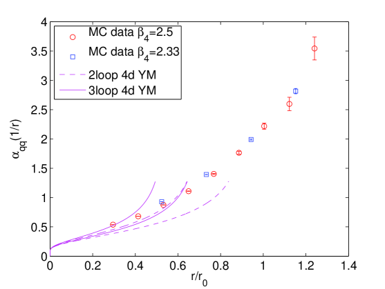
Figure 14: The coupling $\alpha_{\rm qq}$ Eq. (2.17) at the bulk phase transition in the confined vacuum. The simulations have been performed at $\beta_{4}=2.33,\;2.5$, cf Table 2.

The simulation results presented in the previous section show that at $\gamma<1$ dimensional reduction from five to four dimensions can occur by compactifying one of the directions orthogonal to the fifth dimension. We discovered that the relevant degrees of freedom (the broken Polyakov loops) fluctuate almost independently when defined in the hyperplanes orthogonal to the extra dimension. The theory in the broken phase reduces to four dimensions and not three, thereby indicating that the hyperplanes do not exactly decouple but some interaction is left. Here we go back to simulations of the theory in “infinite volume”. By this we mean that all five directions are larger than their minimal size, see Eq. (4.24). If the hyperplanes decouple, the theory reduces to four dimensions, as is the case in the mean-field computation of [?].

We computed the static potential $V(r)$ along spatial directions orthogonal to the extra dimension (and averaged over the extra dimension). In the deconfined phase (where the Polyakov loops are broken) it is a five-dimensional Coulomb potential [?]. Here we choose parameters which correspond to bulk phase transition points and we put ourselves approximately in the middle of the hysteresis curve. We started the simulations with a hot start in order to stay in the vacuum of the confined phase and we checked that the Polyakov loop expectation values are indeed zero in all directions. We choose the points in parameter space $(\beta_{4}=2.33,\beta_{5}=0.937)$ and $(\beta_{4}=2.5,\beta_{5}=0.8697)$, cf Fig. 8, and the lattice size is $32^{4}\times 16$. We ran 4 replica at $\beta_{4}=2.33$ and 11 replica at $\beta_{4}=2.5$ for a total of 38280 and 103410 measurements respectively. Each replicum used 512 cores of the supercomputer Cheops of the University of Cologne and consists of $10^{4}$ update iterations (each iteration does one heatbath and 16 overrelaxation sweeps) for thermalization and approximately $10^{4}$ measurements of the Wilson loops separated by 10 update iterations. We take four levels of HYP smearing for the spatial links of the Wilson loops. We measure the potential starting from distance $r=2a_{4}$ and the force from $r=2.5a_{4}$. For the fit of the effective masses in Eq. (2.14) we use the range $t=2,3,\ldots,6$. The values of the scale $r_{0}/a_{4}$ are given in Table 2. At $\beta_{4}=2.5$ the lattice spacing $a_{4}$ is almost half the one at $\beta_{4}=2.33$.

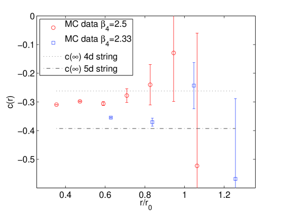
Figure 15: The slope $c$ Eq. (2.18) at the bulk phase transition in the confined vacuum, from the same simulations as in Fig. 14.

In Fig. 14 we show the coupling $\alpha_{\rm qq}$ Eq. (2.17) as a function of $r/r_{0}$, square symbols for $\beta_{4}=2.33$ and circles for $\beta_{4}=2.5$. The string tension is estimated to be $\sigma r_{0}^{2}=1.3(2)$ and $\sigma r_{0}^{2}=1.4(2)$ at $\beta_{4}=2.33$ and $\beta_{4}=2.5$ respectively. We plot the 2-loop (dashed) and 3-loop (solid) perturbative curves for the SU(2) Yang–Mills theory in four dimensions, as explained in Appendix A. The points at the smallest distances are compatible with the 3-loop running, especially on the finer lattice at $\beta_{4}=2.5$.

Fig. 15 presents the analysis of the slope $c(r)$ Eq. (2.18). At $\beta_{4}=2.33$ the values of $c$ seem to be more compatible with the five-dimensional value of the Lüscher coefficient (marked by a horizontal dashed-dotted line). As we lower the lattice spacing $a_{4}$, at $\beta_{4}=2.5$ the data have a clear trend towards the four-dimensional value of the Lüscher coefficient (marked by a horizontal dotted line). We loose the statistical signal above distance $r=r_{0}$. But as was noticed in [?] the onset of the string behavior in the static potential starts already at distance $r_{0}$. There is no scaling between the two simulations and we are most probably not on a line of constant physics. We interpret our results as an indication that increasing $\beta_{4}$ along the bulk phase transition line makes the theory more four-dimensional than five-dimensional, hinting at a dynamical localization mechanism for the gauge field.

It is not clear whether there exists a continuum limit when $\beta_{4}$ increases while staying in the confined phase at $\gamma<1$. But even if it does not exist, there could be a window of values of the lattice spacing for which the cut-off effects are small and the five-dimensional gauge theory can be described by an effective four-dimensional theory for energies much smaller than the cut-off.

5 Conclusions

Lattice gauge theory is the tool to explore five-dimensional gauge theories away from their trivial limit. So far we did not find in Monte Carlo simulations of gauge group SU(2) using the anisotropic Wilson gauge action and periodic boundary conditions a second order bulk phase transition where a continuum limit could be taken. We located a line of first order bulk phase transitions separating the confined from the deconfined phase. In this article we studied in particular the phase diagram for anisotropy $\gamma<1$ (where the lattice spacing $a_{5}$ is larger than $a_{4}$). As we move along the bulk phase transition line, while decreasing $a_{4}$ and staying in the large volume confined phase, we find indications of dimensional reduction. Dimensional reduction at $\gamma<1$ was previously found in a mean-field calculation [?] and relied on a decoupling of the hyperplanes orthogonal to the extra dimension. This effect is seen in our analyses of second order phase transitions related to breaking of the center. At these transitions our finite size scaling studies are perfectly compatible with the critical exponent of the four-dimensional Ising model.

As a next step we would like to measure the mass spectrum in the scalar and vector channels in order to understand what exactly is the (almost) four-dimensional theory that we get in the hyperplanes orthogonal to the extra dimension at $\gamma<1$. These studies prepare the ground for future simulations of the theory with orbifold boundary conditions [?,?,?].

Acknowledgement. This work was funded by the Deutsche Forschungsgemeinschaft (DFG) under contract KN 947/1-1. In particular A. R. acknowledges full support from the DFG. We thank Nikos Irges and Björn Leder for their inputs during discussions. The Monte Carlo simulations were carried out on the Cheops supercomputer at the RRZK computing centre of the University of Cologne and on the cluster Stromboli at the University of Wuppertal and we thank both Universities.

Appendix A Perturbation theory in the qq-scheme

We summarize the steps needed to compute the 3-loop running of

$$\bar{g}_{\mathrm{qq}}^{2}(\mu) = \frac{4\pi}{C_{\rm F}}r^{2}F(r)\,,\;\mu=1/r\,,$$ (A.25)

where $C_{\mathrm{F}}=(N^{2}-1)/(2N)$, in the SU(N) Yang–Mills theory in four dimensions. The beta function is defined by the renormalization group equation

$$\mu\frac{{\rm d}}{{\rm d}\mu}\bar{g}_{\mathrm{qq}}(\mu) = \beta_{\mathrm{qq}}(\bar{g}_{\mathrm{qq}}(\mu))$$ (A.26)

and has the perturbative expansion

$$\beta_{\mathrm{qq}}(\bar{g}_{\mathrm{qq}}) = -\bar{g}_{\mathrm{qq}}^{3}\left(b^{\rm(qq)}_{0}+b^{\rm(qq)}_{1}\bar{g}_{\mathrm{qq}}^{2}+b^{\rm(qq)}_{2}\bar{g}_{\mathrm{qq}}^{4}\ldots\right)\,.$$ (A.27)

The coefficients ($C_{\rm A}=N$)

$$b^{\rm(qq)}_{0}=b_{0} = \frac{1}{(4\pi)^{2}}11C_{\rm A}/3\,,$$ (A.28)

$$b^{\rm(qq)}_{1}=b_{1} = \frac{1}{(4\pi)^{4}}34C_{\rm A}^{2}/3\,,$$ (A.29)

are universal. The 3-loop coefficient

$$b^{\rm(qq)}_{2} = \frac{C_{\rm A}^{3}}{(4\pi)^{6}}\left(\frac{206}{3}+\frac{44\pi^{2}}{3}-\frac{11\pi^{4}}{12}+\frac{242}{9}\zeta(3)\right)+\left(\frac{\pi^{2}}{3}-4\right)b_{0}^{3}$$ (A.30)

is determined combining results from [?,?]. In order to integrate Eq. (A.26) we evaluate numerically

$$\frac{\Lambda_{\mathrm{qq}}}{\mu} = \left(b_{0}\bar{g}_{\mathrm{qq}}^{2}\right)^{-b_{1}/(2b_{0}^{2})}{\rm e}^{-1/(2b_{0}\bar{g}_{\mathrm{qq}}^{2})}\exp\left\{-\int_{0}^{\bar{g}_{\mathrm{qq}}}{\rm d}x\left[\frac{1}{\beta_{\mathrm{qq}}(x)}+\frac{1}{b_{0}x^{3}}-\frac{b_{1}}{b_{0}^{2}x}\right]\right\}\,,$$

where for $\beta_{\mathrm{qq}}$ we insert the truncated perturbative expansion.

For the evaluation of Eq. (LABEL:e_lambdapar) we need to know the Lambda-parameter in the qq-scheme. For gauge group SU(2) it can be estimated from the data of the Schrödinger Functional (SF) coupling in Table 5 of [?]. We integrate Eq. (LABEL:e_lambdapar) in the SF scheme using the $b_{2}^{\rm SF}$ coefficient determined in [?,?]. We take the smallest coupling from [?] and use the determination of the $r_{0}$ scale in [?]. After converting to the qq-scheme [?] we estimate

$$\Lambda_{\mathrm{qq}}\,r_{0} = 0.80(11)$$ (A.32)

from the 3-loop running (which agrees with the 2-loop result).

References

- [1] M. Creutz, Phys. Rev. Lett. 43 (1979) 553.
- [2] K.G. Wilson, Phys.Rev. D10 (1974) 2445.
- [3] S. Ejiri, J. Kubo and M. Murata, Phys.Rev. D62 (2000) 105025, hep-ph/0006217.
- [4] S. Chandrasekharan and U. Wiese, Nucl.Phys. B492 (1997) 455, hep-lat/9609042.
- [5] B. Schlittgen and U. Wiese, Phys.Rev. D63 (2001) 085007, hep-lat/0012014.
- [6] P. de Forcrand, A. Kurkela and M. Panero, JHEP 06 (2010) 050, 1003.4643.
- [7] D.B. Kaplan, Phys.Lett. B288 (1992) 342, hep-lat/9206013.
- [8] M. Lüscher, (2000) 41, hep-th/0102028.
- [9] G. Dvali and M.A. Shifman, Phys.Lett. B396 (1997) 64, hep-th/9612128.
- [10] M. Laine, H. Meyer, K. Rummukainen and M. Shaposhnikov, JHEP 0404 (2004) 027, hep-ph/0404058.
- [11] Y. Fu and H.B. Nielsen, Nucl.Phys. B236 (1984) 167.
- [12] P. Dimopoulos, K. Farakos and S. Vrentzos, Phys.Rev. D74 (2006) 094506, hep-lat/0607033.
- [13] CMS Collaboration, S. Chatrchyan et al., JHEP 1105 (2011) 093, 1103.0981.
- [14] ATLAS Collaboration, G. Aad et al., Phys.Lett. B700 (2011) 163, 1103.6218.
- [15] N. Irges and F. Knechtli, Nucl.Phys. B822 (2009) 1, 0905.2757.
- [16] N. Irges and F. Knechtli, Phys.Lett. B685 (2010) 86, 0910.5427.
- [17] J.M. Drouffe and J.B. Zuber, Phys.Rept. 102 (1983) 1.
- [18] W. Rühl, Z.Phys. C18 (1983) 207.
- [19] H. Gies, Phys.Rev. D68 (2003) 085015, hep-th/0305208.
- [20] T.R. Morris, JHEP 0501 (2005) 002, hep-ph/0410142.
- [21] N. Irges and F. Knechtli, Nucl.Phys. B719 (2005) 121, hep-lat/0411018.
- [22] K.R. Dienes, E. Dudas and T. Gherghetta, Nucl.Phys. B537 (1999) 47, hep-ph/9806292.
- [23] N. Irges, F. Knechtli and M. Luz, JHEP 0708 (2007) 028, 0706.3806.
- [24] K. Fabricius and O. Haan, Phys. Lett. B143 (1984) 459.
- [25] A. Kennedy and B. Pendleton, Phys.Lett. B156 (1985) 393.
- [26] I. Montvay and G. Münster, Quantum Fields on a Lattice (Cambridge University Press, 1994).
- [27] M. Creutz, Phys.Rev. D21 (1980) 2308.
- [28] ALPHA, U. Wolff, Comput. Phys. Commun. 156 (2004) 143, Erratum-ibid.176:383,2007, hep-lat/0306017.
- [29] K. Binder, Z.Phys. B43 (1981) 119.
- [30] G. Parisi, R. Petronzio and F. Rapuano, Phys. Lett. B128 (1983) 418.
- [31] A. Hasenfratz and F. Knechtli, Phys.Rev. D64 (2001) 034504, hep-lat/0103029.
- [32] C.W. Bernard and T.A. DeGrand, Nucl. Phys. Proc. Suppl. 83 (2000) 845, hep-lat/9909083.
- [33] M. Donnellan, F. Knechtli, B. Leder and R. Sommer, Nucl.Phys. B849 (2011) 45, 1012.3037.
- [34] R. Sommer, Nucl.Phys. B411 (1994) 839, hep-lat/9310022.
- [35] M. Lüscher and P. Weisz, JHEP 0207 (2002) 049, hep-lat/0207003.
- [36] M. Lüscher, K. Symanzik and P. Weisz, Nucl. Phys. B173 (1980) 365.
- [37] M. Lüscher, Nucl. Phys. B180 (1981) 317.
- [38] C. Lang, M. Pilch and B. Skagerstam, Int.J.Mod.Phys. A3 (1988) 1423.
- [39] C. Bonati, G. Cossu, M. D’Elia and A. Di Giacomo, Nucl.Phys. B828 (2010) 390, 0911.1721.
- [40] M.E.J. Newman and G.T. Barkema, Monte Carlo Methods in Statistical Physics (Claredon Press, Oxford University Press, 2001).
- [41] B. Svetitsky and L.G. Yaffe, Nucl.Phys. B210 (1982) 423.
- [42] K. Farakos and S. Vrentzos, (2010), 1007.4442.
- [43] F. Knechtli, N. Irges and A. Rago, PoS LATTICE2010 (2010) 059, 1011.0345.
- [44] N. Irges and F. Knechtli, Nucl.Phys. B775 (2007) 283, hep-lat/0609045.
- [45] K. Ishiyama, M. Murata, H. So and K. Takenaga, Prog.Theor.Phys. 123 (2010) 257, 0911.4555.
- [46] M. Peter, Nucl. Phys. B501 (1997) 471, hep-ph/9702245.
- [47] Y. Schröder, Phys. Lett. B447 (1999) 321, hep-ph/9812205.
- [48] M. Lüscher, R. Sommer, U. Wolff and P. Weisz, Nucl.Phys. B389 (1993) 247, hep-lat/9207010.
- [49] M. Lüscher and P. Weisz, Phys.Lett. B349 (1995) 165, hep-lat/9502001.
- [50] R. Narayanan and U. Wolff, Nucl.Phys. B444 (1995) 425, hep-lat/9502021.