THE GEOMETRY OF THE QUANTUM ZENO EFFECT

Abstract

The quantum Zeno effect is described in geometric terms. The quantum Zeno time (inverse standard deviation of the Hamiltonian) and the generator of the quantum Zeno dynamics are both given a geometric interpretation.

1 Introduction and dedication

According to Wikipedia [1], a dedication “refers to the inscription of books or other artifacts when these are specifically addressed or presented to a particular person. This practice, which once was used to gain the patronage and support of the person so addressed, is now only a mark of affection or regard. In law, the word is used of the setting apart by a private owner of a road to public use.”

We do neither intend to gain Beppe Marmo’s support, nor show him our (long-standing) affection and regard. Rather, we shall adopt the afore-mentioned jurisdictional connotation of the word “dedication”. There is a road to understanding physics that makes use of geometry. Einstein was a precursor in the field. Beppe has been for a long time an outstanding advocate of such a geometric understanding. On many different occasions, we have discussed with him the basic notions of the quantum Zeno effect [2]. A geometrical picture of such a fundamental quantum mechanical effect was proposed by Beppe at the conference for the 75th birthday of George Sudarshan [3], who fathered the quantum Zeno effect (QZE) in a seminal article written in collaboration with Baidyanath Misra [4].

The objective of this note is to discuss this geometric road to the QZE, both in general terms and by making use of a concrete example. In jurisdictional terminology, the “dedication” is therefore by Beppe to public use, and to the authors of this article in particular. The effect of a dedication is that the freehold of the road is transferred to the public, who can avail themselves of it. In physics (unlike with roads) this has a price, in that one has to learn how to speak the beautiful language of geometry. Beppe is aware of it. In fact we suspect that this was his original plan: to inculcate his friends with the love of the geometrical language and approach to quantum mechanics.

2 Quantum Zeno effect and quantum Zeno dynamics

Consider a quantum system described in a Hilbert space $\mathcal{H}$, whose dynamical evolution is governed by a Hamiltonian operator $H$. Let $|{\psi_{0}}\rangle\in\mathcal{H}$ be its initial condition (pure state). The evolution is

$$|{\psi_{t}}\rangle=\mathrm{e}^{-\mathrm{i}Ht}|{\psi_{0}}\rangle,$$ (2.1)

with $\langle\psi_{0}|\psi_{0}\rangle=1,\langle\psi_{t}|\psi_{t}\rangle=1$. The survival amplitude and probability read

$$A(t)=\langle\psi_{0}|\psi_{t}\rangle=\langle{\psi_{0}}|\mathrm{e}^{-\mathrm{i}Ht}|{\psi_{0}}\rangle,\qquad p(t)=|A(t)|^{2},$$ (2.2)

respectively. At small times

$$p(t)\sim 1-\frac{t^{2}}{\tau_{\mathrm{Z}}^{2}}.$$ (2.3)

The above quadratic behavior stems from first principles and very general features of the Schrödinger equation. The time constant

$$\tau_{\mathrm{Z}}^{-2}=(\triangle H)^{2}=\frac{\langle{\psi_{0}}|H^{2}|{\psi_{0}}\rangle}{\langle\psi_{0}|\psi_{0}\rangle}-\left(\frac{\langle{\psi_{0}}|H|{\psi_{0}}\rangle}{\langle\psi_{0}|\psi_{0}\rangle}\right)^{2}$$ (2.4)

is the Zeno time. We explicitly wrote the norms in Eq. (2.4) in order to make clear that the relevant objects belong to the complex projective space $\mathbb{P}\mathcal{H}$.

Let $P$ be a projection onto $\mathcal{H}_{P}=P\mathcal{H}$ and $|{\psi_{0}}\rangle=P|{\psi_{0}}\rangle$ (state preparation). The evolution after $N$ projective measurements at time intervals $t/N$ reads

$$|{\psi_{t}^{(N)}}\rangle=V_{N}(t)|{\psi_{0}}\rangle,\qquad V_{N}(t)=V(t/N)^{N}=(PU(t/N)P)^{N}.$$ (2.5)

Notice that $|{\psi_{t}^{(N)}}\rangle$ is not normalized. We are interested in the $N\to\infty$ limit of the above evolution. The general case (unbounded $H$, infinite-dimensional $P$) is still open [5]. However, if $H$ is bounded and/or $P$ finite-dimensional, the limiting evolution is unitary and readily computed:

$$|{\psi_{t}^{(\textrm{Z})}}\rangle=U_{\textrm{Z}}(t)|{\psi_{0}}\rangle,\qquad U_{\textrm{Z}}(t):=\lim_{N\to\infty}V_{N}(t)=\mathrm{e}^{-\mathrm{i}H_{\textrm{Z}}t}P,\qquad H_{\textrm{Z}}:=PHP.$$ (2.6)

The (self-adjoint) generator $H_{\textrm{Z}}$ is called Zeno Hamiltonian and the above equation defines the (unitary) quantum Zeno dynamics. Our main objectives will be to gain a geometrical intepretation of the Zeno time (2.4) and of the Zeno Hamiltonian (2.6). An attempt to interpret the Zeno time in geometrical terms was done in [6].

3 Geometry of quantum mechanics

States are not vectors $|\psi\rangle\in\mathcal{H}$ but rather rays, elements of the Hilbert manifold $\mathbb{P}\mathcal{H}$, which can conveniently parametrized as rank-one projection operators. This projection map enables one to identify on $\mathbb{P}\mathcal{H}$ a metric tensor, usually called the Fubini-Study metric, and a symplectic structure [7, 8]. Both of them define on $\mathbb{P}\mathcal{H}$ what is called a Kählerian structure. To work with this tensor on $\mathcal{H}$ instead of $\mathbb{P}\mathcal{H}$ is quite convenient for computational purposes.

We shall consider finite dimensional systems. Let $\mathcal{H}\simeq\mathbb{C}^{n}$ and introduce the orthornormal basis $\{|{e_{1}}\rangle,\dots,|{e_{n}}\rangle\}$ and coordinates $z_{k}=(q_{k}+\mathrm{i}p_{k})$. This entails

$$\mathcal{H}\to\mathbb{C}^{n}\to\mathbb{R}^{2n},$$ (3.1)

with

$$|{\psi}\rangle\mapsto\left(\begin{array}[]{c}\langle e_{1}|\psi\rangle\\ \langle e_{2}|\psi\rangle\\ \vdots\\ \langle e_{n}|\psi\rangle\end{array}\right)=:\left(\begin{array}[]{c}z_{1}\\ z_{2}\\ \vdots\\ z_{n}\end{array}\right)=:\left(\begin{array}[]{c}q_{1}+\mathrm{i}p_{1}\\ q_{2}+\mathrm{i}p_{2}\\ \vdots\\ q_{n}+\mathrm{i}p_{n}\end{array}\right)\mapsto\left(\begin{array}[]{c}q_{1}\\ \vdots\\ q_{n}\\ p_{1}\\ \vdots\\ p_{n}\end{array}\right).$$ (3.2)

The complex inner product of $\mathcal{H}$ induces the Hermitian structure

$$\mathfrak{h}=\sum_{k}\mathrm{d}\bar{z}_{k}\otimes\mathrm{d}z_{k}=\mathfrak{g}+\frac{\mathrm{i}}{2}\omega,$$ (3.3)

where

$$\mathfrak{g} = \frac{1}{2}\sum_{k}(\mathrm{d}\bar{z}_{k}\otimes\mathrm{d}z_{k}+\mathrm{d}z_{k}\otimes\mathrm{d}\bar{z}_{k})=\sum_{k}\mathrm{d}\bar{z}_{k}\otimes_{s}\mathrm{d}z_{k},$$ (3.4)

$$\omega = -\mathrm{i}\sum_{k}(\mathrm{d}\bar{z}_{k}\otimes\mathrm{d}z_{k}-\mathrm{d}z_{k}\otimes\mathrm{d}\bar{z}_{k})=-\mathrm{i}\sum_{k}\mathrm{d}\bar{z}_{k}\wedge\mathrm{d}z_{k}$$ (3.5)

are a Riemannian metric and a symplectic form, respectively. In terms of the real coordinates, they read

$$\mathfrak{g}=\sum_{k}(\mathrm{d}q_{k}\otimes\mathrm{d}q_{k}+\mathrm{d}p_{k}\otimes\mathrm{d}p_{k}),\qquad\omega=\sum_{k}\mathrm{d}q_{k}\wedge\mathrm{d}p_{k},$$ (3.6)

respectively. Let us introduce the dual coordinate vector fields

$$\frac{\partial}{\partial z_{k}}=\frac{1}{2}\left(\frac{\partial}{\partial q_{k}}-\mathrm{i}\frac{\partial}{\partial p_{k}}\right),\quad\mathrm{d}z_{j}\left(\frac{\partial}{\partial z_{k}}\right)=\frac{\partial}{\partial z_{k}}z_{j}=\delta^{k}_{j},\quad\mathrm{d}\bar{z}_{j}\left(\frac{\partial}{\partial z_{k}}\right)=0$$ (3.7)

and analogously for $\frac{\partial}{\partial\bar{z}_{k}}$. In terms of them we can write the contravariant form of the Hermitian structure:

$$K=\sum_{k}\frac{\partial}{\partial\bar{z}_{k}}\otimes\frac{\partial}{\partial z_{k}}=G+\frac{\mathrm{i}}{2}\Omega,$$ (3.8)

where

$$G = \sum_{k}\frac{\partial}{\partial\bar{z}_{k}}\otimes_{s}\frac{\partial}{\partial z_{k}}=\frac{1}{4}\sum_{k}\left(\frac{\partial}{\partial q_{k}}\otimes\frac{\partial}{\partial q_{k}}+\frac{\partial}{\partial p_{k}}\otimes\frac{\partial}{\partial p_{k}}\right),$$ (3.9)

$$\Omega = -\mathrm{i}\sum_{k}\frac{\partial}{\partial\bar{z}_{k}}\wedge\frac{\partial}{\partial z_{k}}=-\frac{1}{2}\sum_{k}\frac{\partial}{\partial q_{k}}\wedge\frac{\partial}{\partial p_{k}}.$$ (3.10)

By using $\Omega$ we can construct the Hamiltonian vector field $X_{f}$ generated by any (smooth) Hamiltonian function $f$, in the standard way:

$$X_{f}=\Omega(\mathrm{d}f,\cdot)=-\mathrm{i}\sum_{k}\left(\frac{\partial f}{\partial\bar{z}_{k}}\frac{\partial}{\partial z_{k}}-\frac{\partial f}{\partial z_{k}}\frac{\partial}{\partial\bar{z}_{k}}\right)=\frac{1}{2}\sum_{k}\left(\frac{\partial f}{\partial p_{k}}\frac{\partial}{\partial q_{k}}-\frac{\partial f}{\partial q_{k}}\frac{\partial}{\partial p_{k}}\right).$$ (3.11)

It is easy to verify that it satisfies the equation $\omega(X_{f},\cdot)=\mathrm{d}f$. The tensor $\Omega$ defines also a Lie algebra structure on functions, with the Poisson brackets

$$\{f,g\} = \Omega(\mathrm{d}f,\mathrm{d}g)$$ (3.12)

$$= -\mathrm{i}\sum_{k}\left(\frac{\partial f}{\partial\bar{z}_{k}}\frac{\partial g}{\partial z_{k}}-\frac{\partial f}{\partial z_{k}}\frac{\partial g}{\partial\bar{z}_{k}}\right)=\frac{1}{2}\sum_{k}\left(\frac{\partial f}{\partial p_{k}}\frac{\partial g}{\partial q_{k}}-\frac{\partial f}{\partial q_{k}}\frac{\partial g}{\partial p_{k}}\right).$$

On the other hand, $G$ defines a Jordan algebra on all quadratic functions, with the Jordan brackets

$$\{f,g\}_{+} = G(\mathrm{d}f,\mathrm{d}g)$$ (3.13)

$$= \frac{1}{2}\sum_{k}\left(\frac{\partial f}{\partial\bar{z}_{k}}\frac{\partial g}{\partial z_{k}}+\frac{\partial f}{\partial z_{k}}\frac{\partial g}{\partial\bar{z}_{k}}\right)=\frac{1}{4}\sum_{k}\left(\frac{\partial f}{\partial q_{k}}\frac{\partial g}{\partial q_{k}}+\frac{\partial f}{\partial p_{k}}\frac{\partial g}{\partial p_{k}}\right).$$

The real quadratic functions are the expectation values of observables

$$f_{A}(\psi)=\langle{\psi}|A|{\psi}\rangle=\sum_{k,l}\bar{z}_{k}A_{kl}z_{l}.$$ (3.14)

$(\Omega,G)$ defines a Lie-Jordan algebra on these expectation values,

$$\{f_{A},f_{B}\}=f_{\mathrm{i}(AB-BA)},\qquad\{f_{A},f_{B}\}_{+}=f_{\frac{1}{2}(AB+BA)},$$ (3.15)

isomorphic to the Lie-Jordan algebra of the observables.

The Hamilton equations, whose Hamiltonian vector fields (3.11) are generated by quadratic functions $f_{H}=\langle{\psi}|H|{\psi}\rangle$,

$$\dot{z}_{k}=X_{f_{H}}(z_{k})=-\mathrm{i}\frac{\partial f}{\partial\bar{z}_{k}}=-\mathrm{i}\sum H_{kl}z_{l},$$ (3.16)

are nothing but the Schrödinger equation with Hamiltonian operator $H$, $\dot{\psi}=H\psi$. The evolution of any expectation value (3.14) is given in terms of the Poisson brackets

$$\dot{f}_{A}=\{f_{H},f_{A}\}=f_{\mathrm{i}(HA-AH)},$$ (3.17)

which is the Heisenberg equation for the operator $A$, $\langle{\psi}|\dot{A}|{\psi}\rangle=\langle{\psi}|\mathrm{i}(HA-AH)|{\psi}\rangle$.

Projectability onto $\mathbb{P}\mathcal{H}$ requires a conformal factor

$$\tilde{G}(\psi)=\langle\psi|\psi\rangle G(\psi),\qquad\tilde{\Omega}(\psi)=\langle\psi|\psi\rangle\Omega(\psi).$$ (3.18)

Observe that $\tilde{\Omega}$ does not satisfy the Jacobi identity any more. However, it does on expectation values. Thus, $\tilde{\Omega}$ projects onto $\mathbb{P}\mathcal{H}$, a Poisson space. Moreover, one should consider homogeneous expectation values

$$\tilde{f}_{A}=\frac{\langle{\psi}|A|{\psi}\rangle}{\langle\psi|\psi\rangle}.$$ (3.19)

We are now ready to make the first key observation: the Zeno time (2.4) is the inverse length of the Hamiltonian vector field on the complex projective space:

$$\tau_{\mathrm{Z}}^{-2}=\tilde{G}(\mathrm{d}\tilde{f}_{H},\mathrm{d}\tilde{f}_{H}).$$ (3.20)

Indeed, we have

$$\mathrm{d}\tilde{f}_{H}=\frac{1}{\|\psi\|^{2}}\left(\mathrm{d}f_{H}-\tilde{f}_{H}\mathrm{d}\|\psi\|^{2}\right),$$ (3.21)

and from (3.15) we get

$$G(\mathrm{d}f_{H},\mathrm{d}f_{H})=\{f_{H},f_{H}\}_{+}=f_{H^{2}}=\langle{\psi}|H^{2}|{\psi}\rangle.$$ (3.22)

Therefore,

$$\tilde{G}(\mathrm{d}\tilde{f}_{H},\mathrm{d}\tilde{f}_{H}) = \frac{1}{\|\psi\|^{2}}G\left(\mathrm{d}f_{H}-e_{H}\mathrm{d}\|\psi\|^{2},\mathrm{d}f_{H}-e_{H}\mathrm{d}\|\psi\|^{2}\right)$$ (3.23)

$$= \tilde{f}_{H^{2}}-(\tilde{f}_{H})^{2}=(\triangle H)^{2}.$$

4 An example: the qubit

Let $\mathcal{H}\simeq\mathbb{C}^{2}\simeq\mathbb{R}^{4}$ with Hamiltonian

$$H=h_{0}\mathbb{I}+\vec{h}\cdot\vec{\sigma},$$ (4.1)

where $\vec{\sigma}=(\sigma_{x},\sigma_{y},\sigma_{z})$ is the vector of Pauli matrices, $h_{0}\in\mathbb{R}$, and $\vec{h}=(h_{x},h_{y},h_{z})\in\mathbb{R}^{3}$. We introduce coordinates $z_{1},z_{2}$ in the eigenbasis of $\sigma_{z}$, i.e. $\sigma_{z}|{e_{j}}\rangle=(-1)^{j}|{e_{j}}\rangle$, $j=1,2$. The expectation value (3.14) of the Hamiltonian $H$ reads

$$f_{H}=\langle{\psi}|H|{\psi}\rangle=h_{0}u+h_{x}x+h_{y}y+h_{z}z=h_{0}u+\vec{h}\cdot\vec{x},$$ (4.2)

where the quadratic functions $u,x,y,z$ are the expectation values of the Pauli matrices

$$u = f_{\mathbb{I}}=|z_{1}|^{2}+|z_{2}|^{2}=q_{1}^{2}+p_{1}^{2}+q_{2}^{2}+p_{2}^{2},$$

$$x = f_{\sigma_{x}}=\bar{z}_{1}z_{2}+\bar{z}_{2}z_{1}=2(q_{1}q_{2}+p_{1}p_{2}),$$

$$y = f_{\sigma_{y}}=-\mathrm{i}(\bar{z}_{1}z_{2}-\bar{z}_{2}z_{1})=2(q_{1}p_{2}-p_{1}q_{2}),$$

$$z = f_{\sigma_{z}}=|z_{1}|^{2}-|z_{2}|^{2}=q_{1}^{2}+p_{1}^{2}-q_{2}^{2}-p_{2}^{2}.$$ (4.3)

Notice that $u$ and $\vec{x}$ are not independent, since

$$u^{2}=\left(|z_{1}|^{2}+|z_{2}|^{2}\right)^{2}=x^{2}+y^{2}+z^{2}=\vec{x}^{2}.$$ (4.4)

By making use of (4.4) we easily get that the Zeno time (2.4) is

$$\tau_{\mathrm{Z}}^{-2}=\tilde{G}(\mathrm{d}\tilde{f}_{H},\mathrm{d}\tilde{f}_{H})=\tilde{f}_{H^{2}}-(\tilde{f}_{H})^{2}=\vec{h}^{2}-\frac{(\vec{h}\cdot\vec{x})^{2}}{u^{2}}=\frac{(\vec{h}\wedge\vec{x})^{2}}{\vec{x}^{2}},$$ (4.5)

where $\wedge$ is the vector product in $\mathbb{R}^{3}$.

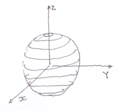
Figure 1: Zeno flow of a qubit subject to measurement $P=\frac{1}{2}(\mathbb{I}+\sigma_{3})$, according to Beppe Marmo, author of the drawing.

Let us now consider the Zeno effect with projection

$$P=|{e_{1}}\rangle\langle{e_{1}}|=\frac{1}{2}(\mathbb{I}+\sigma_{3}).$$ (4.6)

The Zeno dynamics (2.6) becomes

$$U_{\textrm{Z}}(t)=\mathrm{e}^{-\mathrm{i}H_{\textrm{Z}}t}P,\qquad H_{\textrm{Z}}=PHP=\frac{h_{0}+h_{z}}{2}(\mathbb{I}+\sigma_{3}).$$ (4.7)

The Zeno Hamiltonian function reads

$$f_{H_{\mathrm{Z}}}=\frac{h_{0}+h_{z}}{2}(u+z)=(h_{0}+h_{z})|z_{1}|^{2}=(h_{0}+h_{z})(q_{1}^{2}+p_{1}^{2}),$$ (4.8)

which is to be compared to the “free” Hamiltonian function (4.2)-(4.3). The infinitesimal generator of the Zeno dynamics is

$$X_{\mathrm{Z}}=-\mathrm{i}(h_{0}+h_{z})\left(z_{1}\frac{\partial}{\partial z_{1}}-\bar{z}_{1}\frac{\partial}{\partial\bar{z}_{1}}\right)=2(h_{0}+h_{z})\left(p_{1}\frac{\partial}{\partial q_{1}}-q_{1}\frac{\partial}{\partial p_{1}}\right)$$ (4.9)

and the dynamics reads

$$\dot{u}=0,\quad\dot{x}=-2(h_{0}+h_{z})y,\quad\dot{y}=2(h_{0}+h_{z})x,\quad\dot{z}=0.$$ (4.10)

Observe that, due to (4.4), the first equation, $\dot{u}=0$, entails that the flow is on the sphere $|\vec{x}|=$ const. This flow is depicted in Fig. 1.

Notice however that the Zeno dynamics (4.7) implies, through the projection (4.6), also a constraint on the initial condition [state preparation, see the two lines that precede Eq. (2.5)]

$$z_{2}=0\quad\Leftrightarrow\quad x=y=0,\;z>0.$$ (4.11)

Among all possible orbits, the constraint (4.11) “picks” the degenerate orbit on the North Pole and “freezes” the dynamics in the initial state. This is the customary, simplest version of the quantum Zeno effect, obtained through a one-dimensional projection like (4.6). On larger spaces, with multi-dimensional projections, one can obtain non-trivial interesting dynamics [5].

5 Conclusions

We have discussed the quantum Zeno effect and the quantum Zeno dynamics in geometric terms, by proposing a geometric intepretation of the Zeno time (2.4) and of the Zeno Hamiltonian (2.6). The general scheme has been corroborated by the simplest non-trivial quantum-mechanical example, that of a spin-$1/2$ particle. Beppe, who has always considered examples “time consuming” (generalization being the main road towards “understanding”), will hopefully forgive us: the example is his own and it helped us understand. Further generalizations of the scheme described in this note have already been considered by Beppe and will be published elsewhere.

References

- [1] http://en.wikipedia.org/wiki/Dedication
- [2] P. Facchi, V. Gorini, G. Marmo, S. Pascazio and E. C. G. Sudarshan, Phys. Lett. A 275 (2000) 12; P. Facchi, G. Marmo, S. Pascazio, A. Scardicchio and E. C. G. Sudarshan, J. Opt. B: Quantum and Semicl. Optics 6 (2004) S492; P. Facchi, G. Marmo and S. Pascazio, J. Phys.: Conf. Series 196 (2009) 012017.
- [3] “Sudarshan: Seven Science Quests”, Journal of Physics: Conference Series Vol. 196 Number 1 (2009), R. M. Walser, A. P. Valanju and P. M. Valanju Eds.
- [4] B. Misra and E. C. G. Sudarshan, J. Math. Phys. 18 (1977) 756.
- [5] P. Facchi and S. Pascazio, J. Phys. A: Math. Theor. 41 (2008) 493001.
- [6] A. K. Pati and S. V. Lawande, Phys. Rev. A 58 (1998) 831.
- [7] V. I. Man ko, G. Marmo, E. C. G. Sudarshan, F. Zaccaria, Rep. Math. Phys. 55 (2005) 405.
- [8] J. F. Carinena, J. Clemente-Gallardo, G. Marmo, Theor. Math. Phys. 152 (2007) 894.