The imprints of superstatistics in multiparticle production processes

Abstract

We provide an update of the overview of imprints of Tsallis nonextensive statistics seen in a multiparticle production processes. They reveal an ubiquitous presence of power law distributions of different variables characterized by the nonextensivity parameter $q>1$. In nuclear collisions one additionally observes a $q$-dependence of the multiplicity fluctuations reflecting the finiteness of the hadronizing source. We present sum rules connecting parameters $q$ obtained from an analysis of different observables, which allows us to combine different kinds of fluctuations seen in the data and analyze an ensemble in which the energy (E), temperature (T) and multiplicity (N) can all fluctuate. This results in a generalization of the so called Lindhard’s thermodynamic uncertainty relation. Finally, based on the example of nucleus-nucleus collisions (treated as a quasi-superposition of nucleon-nucleon collisions) we demonstrate that, for the standard Tsallis entropy with degree of nonextensivity $q<1$, the corresponding standard Tsallis distribution is described by $q^{\prime}=2-q>1$.

I Introduction

Multiparticle production processes are the main source of our knowledge of the properties of matter formed in extreme conditions. In fact, they are sometimes regarded as an illustration, in laboratory conditions, of the state apparently existing just after the Big Bang. From the very beginning for their investigation it was obvious that the best way of their description and understanding is the approach of statistical mechanics. For a decade now we advocate (see review WW_epja for references) that the quality of data is high enough to observe the deviations from the usual statistical approach based on a Boltzman-Gibbs ensemble towards a more refined one based on its generalization, for example given by Tsallis statistics T ; T2 ; T3 . From the very beginning, we have identified the $q$ parameter occurring in Tsallis statistics with the measure of some intrinsic fluctuations present in the system qWW ; qWW1 . They are natural in systems where the heat bath is not homogeneous. In short: if the scale parameter $\tilde{T}$ (”temperature”) in the usual Boltzman distribution, $f(E)\propto\exp\left(-E/{\tilde{T}}\right)$, fluctuates according to a gamma distribution, $g(1/{\tilde{T}})\propto\left\{T/\left[(q-1)\tilde{T}\right]\right\}^{(2-q)/(q-1)}\exp\left\{-T/\left[(q-1)\tilde{T}\right]\right\}$, with fluctuations given by $q=1+Var(1/\tilde{T})/\langle 1/\tilde{T}\rangle^{2}$, as result one gets the power-like Tsallis distribution:

$$h_{q}(E)=\frac{2-q}{T}\exp_{q}\left(-\frac{E}{T}\right)=\frac{2-q}{T}\left[1-(1-q)\frac{E}{T}\right]^{\frac{1}{1-q}}.$$ (1)

This was quickly recognized as an example of so called superstatistics sS ; sS1 and, in what follows, we shall understand it in this way, i.e., we shall mainly concentrate on the notion of fluctuations represented by the parameter $q$.

The conclusion of qWW ; qWW1 was reinforced by a more refined analysis in BJ ; BJ1 and generalized in WW_epja by additionally allowing for the heat bath to exchange energy with its surroundings. One then gets the same Tsallis distribution as before, but with a $q$-dependent effective temperature, $T_{eff}=T+(q-1)T_{*}$, replacing $T$ in Eq. (1). Here $T_{*}$ is a new parameter depending on the transport properties of the space surrounding the emission region. In WW_epja , where this concept was first introduced for heavy ion collisions, $T_{*}=\phi/(Dc_{P}\rho)$, $\phi$ is the energy transfer taking place between the source and its surroundings. This quantity is supposed to model the possible transfer of energy from the central region of nucleus-nucleus interaction towards the spectators not participating in the collision (when $T_{*}<0$).

For nuclear collisions the possible transfer of energy between the region of interaction and the spectators depends on its size (or on centrality of the reaction). Accounting for it thus explains automatically the observed $q$-dependence of the multiplicity fluctuations measured in nuclear collisions on the centrality of collision WWprc (cf. also qcompilation ). Assuming that the size of the thermal system produced in heavy ion collisions is proportional to the number of nucleons participating in collision, $N_{P}$, one gets that ($C_{V}$ is heat capacity under constant volume)

$$q-1=\frac{1}{aN_{P}}\left(1-\frac{N_{P}}{A}\right),\qquad a=\frac{C_{V}}{N_{P}}$$ (2)

which nicely fits the data WWprc .

Since the review WW_epja , Tsallis distributions have been used more widely, for example, they were successfully applied to the analysis of the recent PHENIX PHENIX and LHC CMS LHC_CMS ; LHC_CMS1 data (cf. also compilation qcompilation ). In what follows we present our recent results in this field in more detail: a derivation of $q$-sum rules unifying different fluctuations - in Section II, a generalization of thermodynamic uncertainty relations and their applications - in Section III. Section IV contains our present result, namely, using as an example the experimental data on nucleus-nucleus collisions (treated as quasi-superposition of nucleon-nucleon collisions), we demonstrate the interrelation between nonextensivity parameters obtained from Tsallis entropy and Tsallis distributions. Section V summarizes our work.

II $q$-sum rules

As argued above, the parameter $q$ provides a useful measure of intrinsic (nonstatistical) fluctuations in the system qWW . In multiparticle production processes the particles produced are characterized by their positions in phase space, in particular the measured momentum $\vec{p}$ is decomposed into longitudinal component (along the direction of colliding particles), $p_{L}=m_{T}\sinh y$, and transverse component, $p_{T}$, with $p=\sqrt{|\vec{p}^{2}|}=\sqrt{p^{2}_{L}+p_{T}^{2}}$ (here $m_{T}=\sqrt{m^{2}+p_{T}^{2}}$ denotes the so called ”transverse mass” of the particle and $y=\frac{1}{2}\ln\frac{E+p_{L}}{E-p_{L}}$ its ”rapidity”; $E$ is the energy of the particle and $m$ is its mass). Because in most cases data are presented in the form of distributions in rapidity $y$ (i.e., they are integrated over $p_{T}$), $dN/dy$, and as distributions in $p_{T}$ (i.e., they are integrated over $y$), $dN/dp_{T}$, one is confronted with two different fluctuations: in longitudinal phase space, characterized by $q=q_{L}$, and in transverse phase space characterized by $q=q_{T}$. It turns out that the strengths of both fluctuations measured by $q$ is different, whereas $q_{L}-1\sim 0.1-0.3$ and grows with energy of collision (measured mainly in $pp$ and ${\bar{p}}p$ collisions), transverse fluctuations are much weaker, $q_{T}-1\sim 0.01-0.1$, vary slowly with energy and depend slightly on whether one observes elementary collisions or collisions between nuclei QlQt2 ; QlQt3 ; MB1 ; MB2 .

There is another source of knowledge concerning fluctuations, namely observed multiplicity distributions, $P(N)$. It turns out that temperature fluctuations in the form of a gamma distribution leading to Eq. (1) result in substantial broadening of the corresponding multiplicity distributions. This changes from poissonian form characteristic for exponential distributions, $P(N)=\bar{N}^{N}\exp\left(-\bar{N}\right)/N!$ (where $\bar{N}=E/T$), to negative binomial form (NB) for Tsallis distributions, Eq. (1) (cf., fluct , for details),

$$P(N)\,=\,\frac{\Gamma(N+k)}{\Gamma(N+1)\Gamma(k)}\frac{\left(\frac{\langle N\rangle}{k}\right)^{N}}{\left(1+\frac{\langle N\rangle}{k}\right)^{(N+k)}};\quad{\rm where}\quad k=\frac{1}{|q-1|}.$$ (3)

The nonextensivity parameter $q$ reflects here fluctuations in the whole of phase space and can be (and usually is), different from the previously obtained $q_{L}$ and $q_{T}$. In QlQt2 ; QlQt3 it was proposed that because $q-1=\sigma^{2}(T)/T^{2}$ (i.e., it is given by fluctuations of total temperature $T$), then assuming that $\sigma^{2}(T)=\sigma^{2}(T_{L})+\sigma^{2}(T_{T})$, the resulting values of $q$ should not be too different from

$$q\,=\,\frac{q_{L}\,T_{L}^{2}\,+\,q_{T}\,T^{2}_{T}}{T^{2}}\,-\,\frac{T^{2}_{L}\,+\,T^{2}_{T}}{T^{2}}\,+\,1.$$ (4)

Therefore for the observed dominance of longitudinal (partition) temperature over the transverse one, $T_{L}\gg T_{T}$, one should expect that $q\sim q_{L}$, which is indeed observed QlQt2 ; QlQt3 . This is the first sum rule observed for parameters $q$ obtained from different measurements.

In cases where other variables in addition to $T$ also fluctuate (usually fluctuations of temperature are deduced either from data averaged over other fluctuations or from data accounting also for fluctuations of other variables) one should refine the experimentally evaluated $q$. In this case, when extracting $q$ from distributions of $dN/dy$, one finds that (cf., WWW for details)

$$q-1\stackrel{{\scriptstyle def}}{{=}}\frac{Var(T)}{\langle T\rangle^{2}}=\frac{Var(z)}{\langle z\rangle^{2}}-\frac{Var\left(m_{T}\right)}{\langle m_{T}\rangle^{2}};\qquad z=\frac{m_{T}}{T}.$$ (5)

This is the second sum rule for parameters $q$ obtained from different measurements. It connects the total $q$, which can be obtained from an analysis of the NB form of the measured multiplicity distributions, $P(N)$, with $q_{L}-1=Var(z)/\langle z\rangle^{2}$, obtained from fitting rapidity distributions and $Var\left(m_{T}\right)/\langle m_{T}\rangle^{2}$ obtained from data on transverse mass distributions. When extracting $q$ from distributions of $dN/dm_{T}$, we proceed analogously with $z=\cosh y/T$.

III Generalized thermodynamic uncertainty relations

We shall continue the above discussion introducing the notion of thermodynamic uncertainty relations and proposing their generalization with the help of nonextensive statistics GTR . They were discussed in BH where it was suggested that the temperature $T$ and energy $U$ could be regarded as being complementary in the same way as energy and time are in quantum mechanics. A simple dimensional analysis suggests that $\Delta U\,\Delta\beta\geq k$, where $\beta=1/T$ and $k$ is Boltzmann’s constant. Isolation ($U$ definite) and contact with a heat bath ($T$ definite) are then the two extreme cases of such complementarity. This is known as Lindhard’s uncertainty relation between the fluctuations of $U$ and $T$ JL :

$$\omega_{U}^{2}\,+\,\omega^{2}_{T}\,=\,\frac{1}{\langle N\rangle}\qquad{\rm where}\qquad\omega^{2}_{x}=Var(x)/\langle x\rangle^{2}.$$ (6)

This idea is still disputable UL ; UL1 ; UL2 , nevertheless we can treat these increments as a measure of fluctuations of the corresponding physical quantities. This allows us to analyze an ensemble in which the energy ($U$), temperature ($T$) and multiplicity ($N$), can all fluctuate and thus to express these fluctuations by the corresponding parameters $q$. In this way, using generalized thermodynamics (based on nonextensive statistics) one gets the following relation GTR

$$\Big{|}\omega^{2}_{N}-\frac{1}{\langle N\rangle}\Big{|}=\omega^{2}_{U}+\omega^{2}_{T}-2\rho\omega_{U}\omega_{T}=\left(\omega_{U}-\omega_{T}\right)^{2}+2\omega_{U}\omega_{T}(1-\rho)=|q-1|,$$ (7)

where $\rho=\rho(U,T)\in[-1,1]$ is the correlation coefficient between $U$ and $T$. This generalizes Linhard’s thermodynamic uncertainty relation.

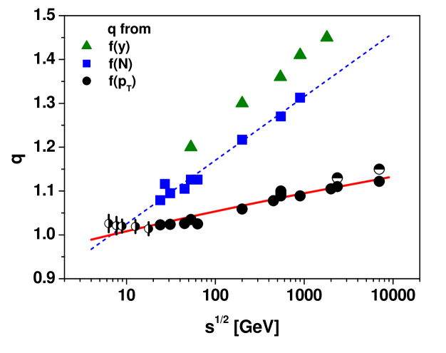
Figure 1: (Color online) Energy dependencies of the parameters $q$ obtained from different observables. Triangles: $q$ obtained from an analysis of rapidity distributions QlQt1 ; rapidity . Squares: $q$ obtained from multiplicity distributions $P(N)$ mult ; mult1 (fitted by $q=1+1/k$ with $1/k=-0.104+0.029\ln s$). Circles: $q$ obtained from different analysis of transverse momenta distribution $f(p_{T})$. Data points in this case come, respectively, from the compilation of $p+p$ data (full symbols) Wibig , from CMS data (half filled circles at high energies) LHC_CMS ; LHC_CMS1 and from NA49 data from Pb+Pb collisions (half filled circles at low energies) NA49 ; NA49-1 ; NA49-2 . The full line comes from our recalculation using Eq.(7).

The observed systematics in energy dependence of the parameter $q$ deduced from presently available data is shown in Fig. 1. From measurements of different observables one observes that for high enough energies $q>1$ (for low energies conservation laws are important and one can encounter $q<1$ situations) and that values of $q$ found from different observables are different. The later is caused either by technical (methodical) problems or else from some physical cause. The former arises when, for example, fluctuations of temperature are deduced either from data averaged over other fluctuations or from more refined data also accounting for fluctuations of other variables (as in WWW , see Eq. (5)). The latter case is connected with the fact that the observed $q$’s were obtained in different parts of phase space (or both). In this case one gets an uncertainty relation (7) with the help of which one can connect fluctuations observed in different parts of phase space. For example, one can recalculate $q$ obtained from $P(N)$ (dashed line in Fig. 1) to $q$ which can be evaluated from $f(p_{T})$ (full line in Fig. 1), see GTR for details.

IV Nonadditivity in nuclear collisions (on the $q$ duality in nonextensive statistics)

So far we were using Tsallis statistics without really resorting to Tsallis entropy, i.e., we treated it as a kind of superstatistics sS ; sS1 . However, closer inspection of both approaches reveals that corresponding nonextensivity parameters (say $q$ and $q^{\prime}$, respectively) are not the same, in fact one encounters a sort of duality, like $q=2-q^{\prime}$ discussed, for example, in KGG ; BJ ; BJ1 . We shall now address this problem in more detail on the example of nonadditivity observed in nuclear collisions where, as we shall see, both types of $q$ can be discussed and (in principle) compared at the same time .

One of the phenomenological approaches used to describe these collisions is based on superposition models in which the main ingredients are nucleons which have interacted at least once WNM . In this case, when sources are identical and independent of each other, the total ($N$) and the mean ($\langle N\rangle$) multiplicities are supposed to be given by,

$$N=\sum_{i=1}^{\nu}n_{i},\qquad{\rm and}\qquad\langle N\rangle=\langle\nu\rangle\langle n_{i}\rangle,$$ (8)

where $\nu$ denotes the number of sources and $n_{i}$ the multiplicity of secondaries from the $i^{th}$ source. Albeit at present nuclear collisions are mostly described by different kinds of statistical models MG_rev , which automatically account for possible collective effects, nevertheless a surprisingly large amount of data can still be described by assuming the above superposition of independent nucleon-nucleon collisions (possibly slightly modified) as the main mechanism of production of secondaries and the question of the range of its validity is a legitimate one FW ; FW1 .

Using the notion of entropy, and considering $\nu$ independent systems for which the corresponding individual probabilities are combined as

$$p^{(\nu)}_{q}\left(x_{1},\dots,x_{(\nu})\right)=\prod_{k=1}^{\nu}p^{(1)}_{q}\left(x_{k}\right),$$ (9)

and assuming that all $p^{(1)}_{q}\left(x_{k}\right)$ are the same for all $k$ (i.e., their corresponding entropies $S_{q}^{(1)}$ are equal), one finds that

$$S_{q}^{(\nu)}=\sum^{\nu}_{k=1}\frac{\nu!}{(\nu-k)!k!}(1-q)^{k-1}\left[S^{(1)}_{q}\right]^{k}=\frac{\left[1+(1-q)S^{(1)}_{q}\right]^{\nu}-1}{1-q}.$$ (10)

In the following we put $\nu=N_{W}/2=N_{P}$ ($N_{W}$ is the number of wounded nucleons and $N_{P}$ is the number of participants from a projectile). Assuming naively that the total entropy is proportional to the mean number of produced particles,

$$S=\alpha\langle N\rangle,$$ (11)

one obtains the following relation between mean multiplicities in $AA$ and $NN$ collisions,

$$\alpha\langle N\rangle_{AA}=\frac{\left[1+(1-q)\alpha\langle N\rangle_{pp}\right]^{N_{P}}-1}{1-q}.$$ (12)

At this point we stress the following important observation, so far not discussed in detail. Namely, because (as shown in WWprc ), $\langle N\rangle_{AA}$ increases nonlinearly with $N_{P}$ and $\langle N\rangle_{AA}>N_{P}\cdot\langle N\rangle_{pp}$, the nonextensivity parameter obtained here from considering the corresponding entropies must be smaller than unity, $q<1$. On the other hand, all estimations od the nonextensivity parameter (let us denote it by $q^{\prime}$) discussed before lead to $q^{\prime}>1$. This is an apparent $q$ duality in nonextensive statistics, on which we shall concentrate in more detail.

Start with the obvious remark that, strictly speaking, relation (12) is not exactly correct for $S_{q}$. In what follows we denote entropy on the level of particle production by $s$ (and the corresponding nonextensivity parameter by $\tilde{q}$), whereas the corresponding entropies and nonextensivity parameter on the level of $NN$ collisions by $S$ and $q$. From Eq. (10) we have that for $N$ particles

$$s^{(N)}_{\tilde{q}}=\frac{\left[1+\left(1-\tilde{q}\right)s^{(1)}_{\tilde{q}}\right]^{N}-1}{1-\tilde{q}}\stackrel{{\scriptstyle\tilde{q}\rightarrow 1}}{{\longrightarrow}}N\cdot s^{(1)}_{\tilde{q}}=\alpha N,$$ (13)

where $s^{(1)}_{\tilde{q}}=\alpha$ is the entropy of a single particle. In a $A+A$ collision with $\nu$ nucleons participating, Eq. (10) results in

$$S^{(\nu)}_{q}=\frac{\left[1+\left(1-q\right)S^{(1)}_{q}\right]^{\nu}-1}{1-q},$$ (14)

where $S^{(1)}_{q}$ is the entropy of a single nucleon.

Denoting multiplicity in single $N+N$ collision by $n$, the respective entropy is S${}^{(1)}_{q}=S^{(1)}_{\tilde{q}}=\left\{\left[1+\left(1-\tilde{q}\right)s^{(1)}_{\tilde{q}}\right]^{n}-1\right\}/(1-\tilde{q})$, whereas entropy in $A+A$ collision for $N$ produced particles is S${}^{(N)}_{\tilde{q}}=\left\{\left[1+\left(1-\tilde{q}\right)s^{(1)}_{\tilde{q}}\right]^{N}-1\right\}/(1-\tilde{q})$. This means that

$$S^{(N)}_{\tilde{q}}=S^{(\nu)}_{q}.$$ (15)

Figure 2: (Color online)Energy dependence of the charged multiplicity for nucleus-nucleus collisions divided by the superposition of multiplicities from proton-proton collisions (cf. Eq. (19)). Experimental data on multiplicity are taken from compilation PHOBOS .

Notice that parameters $q$ and $\tilde{q}$ are usually not identical. Moreover, from relation (2) one gets that for $NN$ collisions (where $N_{P}=A$) $\tilde{q}=1$. On the other hand, for $\tilde{q}=q$ Eq. (15) corresponds to the situation encountered in superpositions, as in this case one gets that

$$\left[1+(1-q)s^{(1)}_{q}\right]^{N}=\left[1+(1-q)s^{(1)}_{q}\right]^{n\nu}\qquad{\rm or}\qquad N=n\nu.$$ (16)

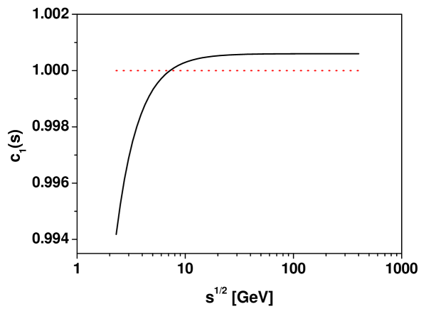
Figure 3: (Color online)Energy ($\sqrt{s}$) dependence of the parameter $c_{1}(s)$ obtained from the analysis of available data.

Consider now the general case and denote

$$c_{1}=1+\left(1-\tilde{q}\right)s^{(1)}_{\tilde{q}};\qquad\qquad c_{2}=\frac{1-q}{1-\tilde{q}}.$$ (17)

These quantities are not independent because:

$$c_{2}c_{1}^{N}+1-c_{2}=\left(c_{2}c_{1}^{n}+1-c_{2}\right)^{\nu}.$$ (18)

From relation (18) one gets that

$$\frac{N}{\nu\cdot n}=\frac{1}{\nu n\cdot\ln c_{1}}\ln\left[\frac{\left(c_{2}c_{1}^{n}+1-c_{2}\right)^{\nu}-\left(1-c_{2}\right)}{c_{2}}\right],$$ (19)

which for $N=\langle N_{AA}\rangle$, $n=\langle N_{pp}\rangle$ and $\nu=N_{P}$ is presented in Fig. 2 for different reactions. As seen there one can describe experimental data by using $c_{2}=1.7$ and with $c_{1}$ depending on energy $\sqrt{s}$ according to $c_{1}(s)=1.0006-0.036s^{-1.035}$, as seen in Fig. 3. Notice that for energies $\sqrt{s}>7$ GeV one has $c_{1}>1$. This means that $\tilde{q}<1$ and (because $c_{2}>0$) also $q<1$.

Now look at this problem from the view point of Tsallis entropy,

$$S_{q}=\frac{1}{1-q}\left[\int dxf^{q}(x)-1\right].$$ (20)

To get from it the probability density function $f(x)$, one either optimizes it with constrains

$$\int dxf(x)=1;\qquad\int dxxf^{q}(x)=\langle x\rangle_{q}$$ (21)

and obtains RS

$$f(x)=(2-q)\left[1-(1-q)x\right]^{\frac{1}{1-q}};\qquad 0\leq x<\infty;\quad 1\leq q\leq 3/2,$$ (22)

or else one uses as constrains

$$\int dxf(x)=1;\qquad\int dxxf(x)=\langle x\rangle$$ (23)

and obtains RS

$$f(x)=\frac{q}{\left[1+(1-q)x\right]^{\frac{1}{1-q}}};\qquad 0\leq x<\infty;\quad 1/2<q\leq 1.$$ (24)

Notice now that only (22) is the same as distribution obtained in superstatistics and used above, cf., Eq. (1). The second distribution, Eq. (24), which seems to be more natural from the point of view of a physical interpretation of the constraint used, becomes the first one if expressed in $q^{\prime}$ given by

$$q^{\prime}=2-q,$$ (25)

namely, in this case one has

$$f(x)=(2-q^{\prime})\left[1-(1-q^{\prime})x\right]^{\frac{1}{1-q^{\prime}}}.$$ (26)

We show here, cf. Fig. 1, that using a Tsallis distribution in the form of Eq. (26), one gets $q^{\prime}>1$. On the other hand, non additivity in the superposition model described using the notion of entropy clearly requires $q<1$, cf. Figs. 2 and 3. This means that $q^{\prime}$ is not the same as $q$. The conclusion one can derive from these considerations is that the second way of deriving $f(x)$, which uses a linear condition, cf. Eq. (24), is the correct one and that $q^{\prime}$ in distribution is not the same as $q$ in entropy. The problem is that, whereas from distributions one can easily deduce a numerical value of $q^{\prime}$, this is not the case when one uses entropy. There are too many variables to play with (cf., considerations using the superposition model as above). For example, in the definition of $c_{1}$ in Eq. (17), one has the $s^{(1)}_{\tilde{q}}$, which is not known a priori. The only thing one can get in this case is that $q<1$. We cannot therefore check numerically that relation (25) really holds. But, if one agrees that the Tsallis distribution comes from Tsallis entropy, we have only two options: either $q^{\prime}=q$ or $q^{\prime}-1=1-q$. Our conclusion presented here, that $q^{\prime}>1$ and $q<1$, therefore supports the second option, i.e., Eq. (25).

V Summary

To summarize, Tsallis statistics is fruitful because in a very economical way (with only one new parameter $q$) it describes the power-like behavior of different observables. This parameter, for $q>1$ considered here, is given fully by nonstatistical fluctuations present in the system and visible as fluctuations of the scale parameter in superstatistics. It also allows (via specific sum rules or through a generalized thermodynamic uncertainty relation) to connect fluctuations of different observables or observed in different parts of phase space. Finally, when considering a superposition scenario, for example, in the scattering of nuclei, the relation $q^{\prime}-1=1-q$ seems to be observed (with $q^{\prime}$ occurring in the Tsallis distribution and $q$ in Tsallis entropy).

This final observation needs some more attention. The probability density function (PDF) is commonly evaluated by the Maximum Entropy Method (MEM) for Tsallis entropy with some constraints OM . At the moment, there are four possible MEMs discussed at length in E6 using two kinds of definition for an expectation value of physical quantities: the normal average (23) and the $q$-average (21) (with normal, as here, or the so-called escort PDFs escort ; escort2 ; escort1 ). Various arguments have been given justifying the $q$-average E11 ; E12 ; E13 . Recently, however, it has been pointed out that, for a small change of the PDF, thermodynamic averages obtained by the $q$-averages are unstable, whereas those obtained by the normal average are stable E14 ; E15 . On the other hand, it is claimed E17 that for the escort PDF, the Tsallis entropy and thermodynamical averages are robust. This means that this issue on the stability (robustness) of thermodynamical averages as well as the Tsallis entropy is still controversial E18 .

References

- (1) M. Gaździcki, M. Gorenstein, P. Seyboth, Acta Phys. Polon. B 42, 307 (2011)
- (2) G. Wilk, Z. Włodarczyk, Eur. Phys. J. A 40, 299 (2009)
- (3) C. Tsallis, Stat. Phys. 52, 479 (1988)
- (4) C. Tsallis, Eur. Phys. J. A 40, 257 (2009)
- (5) C. Tsallis, Introduction to Nonextensive Statistical Mechanics (Springer, 2009)
- (6) G. Wilk, Z. Włodarczyk, Phys. Rev. Lett. 84, 2770 (2000)
- (7) G. Wilk, Z. Włodarczyk, Chaos, Solitons Fractals 13, 581 (2001)
- (8) C. Beck, E. G. D. Cohen, Physica A 322, 267 (2003)
- (9) F. Sattin, Eur. Phys. J. B 49, 219 (2006)
- (10) T. S. Biró, A. Jakovác, Phys. Rev. Lett. 94, 132302 (2005)
- (11) T. S. Biró, G. Purcel, K. Ürmösy, Eur. Phys. J. A 40, 325 (2009)
- (12) G. Wilk, Z. Włodarczyk, Phys. Rev. C 79, 054903 (2009)
- (13) M. Shao et al., J. Phys. G 37, 085104 (2010)
- (14) G. Wilk, Z. Włodarczyk, Cent. Eur. J. Phys. 8, 726 (2010)
- (15) A. Adare et al. (PHENIX Collaboration), Phys. Rev. D 83, 052004 (2011)
- (16) V. Khachatryan et al. (CMS Collaboration), JHEP02, 041 (2010)
- (17) V. Khachatryan et al. (CMS Collaboration), Phys. Rev. Lett. 105, 022002 (2010)
- (18) F. S. Navarra, O. V. Utyuzh, G. Wilk, Z. Włodarczyk, Phys. Rev. D 67, 114002 (2003)
- (19) F. S. Navarra, O. V. Utyuzh, G. Wilk, Z. Włodarczyk, Physica A 340, 467 (2004)
- (20) F. S. Navarra, O. V. Utyuzh, G. Wilk, Z. Włodarczyk, Physica A 344, 568 (2004)
- (21) M. Biyajima, M. Kaneyama, T. Mizoguchi, G. Wilk, Eur. Phys. J. C 40, 243 (2005)
- (22) M. Biyajima, T. Mizoguchi, N. Nakajima, N. Suzuki, G. Wilk, Eur. Phys. J. C 48, 593 (2006)
- (23) G. Wilk, Z. Włodarczyk, Physica A 376, 279 (2007)
- (24) G. Wilk, Z. Włodarczyk, W. Wolak, Acta Phys. Polon. B 42, 1277 (2011)
- (25) G. Wilk, Z. Włodarczyk, Physica A 390, 3566 (2011)
- (26) See: N. Bohr, Collected Works, ed. J. Kalekar (North-Holland, Amsterdam, 1985), Vol. 6, pp. 316-330 and 376-377
- (27) J. Lindhard, ’Complementarity’ between energy and temperature, in The Lesson of Quantum Theory, edited by J. de Boer, E. Dal, O. Ulfbeck (North-Holland, Amsterdam, 1986)
- (28) J. Uffink, J. van Lith, Found. Phys. 29, 655 (1999)
- (29) J. Uffink, J. van Lith, Thermodynamic uncertainty relations, cond-mat/9806102
- (30) B. H. Lavenda, Found. Phys. Lett. 13, 487 (2000)
- (31) M. Rybczyński, Z. Włodarczyk, G. Wilk., Nucl. Phys. B (Proc. Suppl.) 122, 325 (2003)
- (32) A. K. Dash, B. M. Mohanty, J.Phys. G 37, 025102 (2010)
- (33) C. Geich-Gimbel, Int. J. Mod. Phys. A 4, 1527 (1989)
- (34) T. Wibig, J. Phys. G 37, 115009 (2010)
- (35) C. Alt et al., Phys. Rev. C 77, 034906 (2008)
- (36) C. Alt at al., Phys. Rev. C 77, 024903 (2008)
- (37) S. V. Afanasiew et al., Phys. Rev. C 66, 054902 (2002)
- (38) I. V. Karlin, M. Grmela, N. Gorban, Phys. Rev. E 65, 036128 (2002)
- (39) J. Rożynek, G.Wilk, J. Phys. G 36 125108 (2009)
- (40) J. Rożynek, G. Wilk, EPJ Web of Conferences 13, 5002 (2011)
- (41) B. B. Back et al. (PHOBOS Collaboration), Phys. Rev. C 74, 021902(R) (2006)
- (42) A. Białas, M. Błeszynski, W. Czyż, Nucl. Phys. B, 111, 461 (1976)
- (43) K. Fiałkowski, R. Wit, Acta Phys. Pol. B 41, 1317 (2010)
- (44) K. Fiałkowski, R. Wit, Eur. Phys. J. A 45, 51 (2010)
- (45) P. N. Rathie, S. Da Silva, Appl. Math. Sci. 2 no. 28, 1359 ( 2008)
- (46) T. Oikonomou, G. B. Bagci, Phys. Lett. A 374, 2225 (2010)
- (47) C. Tsallis, Physica D 193, 3 (2004)
- (48) C. Beck, F. Schlögl, Thermodynamics of Chaotic Systems (Cambridge Univ. Press, Cambridge, 1993)
- (49) Yu. L. Klimontovich, Statistical Theory of Open Systems (Kluwer, Dordrecht, 1995)
- (50) C. Tsallis, R. S. Mendes, A. R. Plastino, Physica A 261, 534 (1998)
- (51) S. Abe, Phys. Rev. E 66, 046134 (2002)
- (52) S. Abe, Astroph. Space Sci. 305, 241 (2006)
- (53) S. Abe, G. B. Bagci, Phys. Rev. E 71, 016139 (2005)
- (54) S. Abe, Europhys. Lett. 84, 60006 (2008)
- (55) S. Abe, Phys. Rev. E 79, 041116 (2009)
- (56) R. Hanel, S. Thurner, C. Tsallis, Europhys. Lett. 85, 20005 (2009)
- (57) J. F. Lutsko, J. P. Boon, P. Grosfils, Europhys. Lett. 86, 40005 (2009)