Thermal momentum distribution from shifted boundary conditions

Abstract:

At finite temperature the distribution of the total momentum is an observable characterizing the thermal state of a field theory, and its cumulants are related to thermodynamic potentials. In a relativistic system at zero chemical potential, for instance, the thermal variance of the total momentum is a direct measure of the entropy. We relate the generating function of the cumulants to the ratio of a path integral with properly shifted boundary conditions in the compact direction over the ordinary partition function. In this form it is well suited for Monte-Carlo evaluation, and the cumulants can be extracted straightforwardly. We test the method in the SU(3) Yang–Mills theory, and obtain the entropy density at three different temperatures.

1 Introduction

Thermal field theory is the theoretical tool for computing properties of matter at high temperatures and densities from first principles. It allows one, for instance, to determine the equation of state of Quantum Chromodynamics, which in turn is an essential ingredient to understand the properties of matter created in heavy ion collisions, and to model the behavior of hot matter in the early universe (for a review at this conference see Ref. [1]). Obtaining first-principles predictions from a thermal field theory is often challenging since it describes an infinite number of degrees of freedom subject to both quantum and thermal fluctuations. Even though there are several established methods to compute the thermal properties of field theories [2, 3, 4, 5], new theoretical concepts and more efficient computational techniques are still needed in many contexts particularly when weak-coupling methods are inapplicable.

Recently Meyer and I proposed a new way to determine the equation of state of a thermal field theory, and it is the aim of this talk to discuss the results obtained in these papers [6, 7]. We related the generating function of the cumulants of the total momentum distribution to a path integral with properly chosen shifted boundary conditions in the compact direction normalized to the ordinary one. By exploiting the Ward Identities (WIs) associated to the space-time invariances of the continuum theory, the cumulants can be related in a simple manner to thermodynamic potentials. In a relativistic theory at zero chemical potential, for instance, the variance of the momentum probability distribution measures the entropy of the system.

Crucially the argument holds, up to harmless finite-size and discretization effects, also in a lattice box. The formulas are thus applicable at finite lattice spacing and volumes, where ratios of path integrals can be determined by ab initio Monte Carlo computations. As a result the entropy density, the pressure and the specific heat can be obtained by studying the response of the system to the shift, and no additive or multiplicative ultraviolet-divergent renormalizations are needed in taking the continuum limit. We have numerically tested our proposal in the SU(3) Yang–Mills theory, for which the entropy density has been determined at three different temperatures.

2 Momentum distribution from shifted boundaries

For an Euclidean field theory at a temperature $T=1/L_{0}$, where $L_{0}$ is the length of the “time” direction, the relative contribution to the partition function of states with total momentum ${\bf p}$ is given by

$$\frac{R({{\bf p}})}{V}=\frac{{\rm Tr}\{e^{-L_{0}\,\hat{\rm H}}\,\hat{\rm P}^{({{\bf p}})}\}}{{\rm Tr}\{e^{-L_{0}\,\hat{\rm H}}\}}$$ (1)

where $V=L^{3}$ is the spatial volume, and $L$ is the linear dimension in the three spatial directions. The trace in Eq. (1) is over all the states of the Hilbert space, $\hat{\rm P}^{({{\bf p}})}$ is the projector onto those states with total momentum ${\bf p}$, and $\hat{\rm H}$ is the Hamiltonian of the theory. If we introduce the partition function

$$Z({\bf z})=\mathrm{Tr}\{e^{-L_{0}\,\hat{\rm H}}\,e^{i\hat{\bf p}{\bf z}}\}$$ (2)

in which states of momentum ${\bf p}$ are weighted by a phase $e^{i{\bf p}\cdot{\bf z}}$, and we use the standard group theory machinery (see Refs. [8, 9] for a detailed discussion of this point) it easy to show that

$$R({{\bf p}})=\frac{1}{Z}\,\int d^{3}{{\bf z}}\,e^{-i{{\bf p}}\cdot{{\bf z}}}\,Z({\bf z})\;.$$ (3)

The generating function $K({{\bf z}})$ of the cumulants is defined as

$$e^{-K({{\bf z}})}=\frac{1}{V}\sum_{{\bf p}}e^{i{{\bf p}}\cdot{{\bf z}}}\,R({{\bf p}})\;,$$ (4)

and the cumulants are given by

$$k^{{}_{V}}_{\{2n_{1},2n_{2},2n_{3}\}}=(-1)^{n_{1}+n_{2}+n_{3}+1}\,\frac{\partial^{2n_{1}}}{\partial z_{1}^{2n_{1}}}\frac{\partial^{2n_{2}}}{\partial z_{2}^{2n_{2}}}\frac{\partial^{2n_{3}}}{\partial z_{3}^{2n_{3}}}\frac{K({{\bf z}})}{V}\Big{|}_{{\bf z}=0}\;,$$ (5)

where they have been normalized so as to have a finite limit when $V\rightarrow\infty$. The shifted partition function $Z({\bf z})$ can be expressed as an Euclidean path integral with the field satisfying the boundary conditions

$$\phi(L_{0},{{\bf x}})=\pm\phi(0,{{\bf x}}+{{\bf z}})$$ (6)

with the $+$ ($-$) sign for bosonic (fermionic) fields respectively. From Eqs. (3) and (4), the generating function can thus be written as the ratio of partition functions

$$e^{-K({{\bf z}})}=\frac{Z({\bf z})}{Z}\;,$$ (7)

i.e. two path integrals with the same action but different boundary conditions, and the cumulants can be obtained by deriving it with respect to the shift parameter $z$ an appropriate number of times. Being the cumulants the connected correlation functions of the charges associated to the translational invariance of the theory, the functional $K({{\bf z}})$ and the momentum distribution $R({{\bf p}})$ are ultraviolet finite, see Refs. [6, 7] for a comprehensive discussion of this point.

2.1 Extension to the lattice

When defined on a lattice, the theory is invariant under a discrete subgroup of translations and rotations only, the momenta are quantized, and the continuum WIs are broken by discretization effects. Generic lattice definitions of the energy-momentum tensor, as well as the corresponding charges, require ultraviolet renormalization. It is still possible, however, to factorize the Hilbert space of the lattice theory in sectors with definite conserved total momentum. The formula for the lattice projector is given by

$$\hat{\rm P}^{({{\bf p}})}=\frac{a^{3}}{V}\sum_{{\bf z}}\,e^{-i\,{\bf p}\cdot{\bf z}}\,e^{i\,\hat{\bf p}{\bf z}}$$ (8)

where the sum is over all the lattice points. Since only physical states contribute to the symmetry constrained path integrals in Eq. (1) when $L_{0}\neq 0$, the lattice momentum distribution $R({{\bf p}})$ is expected to converge to the continuum universal one without the need for any ultra-violet renormalization. The definition of the cumulants in Eq. (5) is thus applicable at finite lattice spacing, provided the derivatives are replaced with their discrete counterpart, and no additive or multiplicative ultraviolet-divergent renormalization is needed for taking the continuum limit.

2.2 Extension to other symmetries

The factorization of the Hilbert space into sectors whose states have definite transformation properties under a symmetry of the lattice theory is more generally applicable than just for translations. For a generic discrete group, the cubic rotations for instance, the projector onto the states which transform as an irreducible representation $\mu$ is given by

$$\hat{\rm P}^{(\mu)}=\frac{n_{\mu}}{g}\sum_{i=1}^{g}\,\chi^{(\mu)*}({\cal R}_{i})\,\hat{\Gamma}({\cal R}_{i})\;,\qquad\hat{\Gamma}({\cal R}_{i})\,|\phi\rangle=|\phi^{{\cal R}_{i}}\rangle\;,$$

where $n_{\mu}$ is the dimension of the representation, $g$ the order of the group, $\chi^{(\mu)}({\cal R}_{i})$ the character of the irreducible representation for the group element ${\cal R}_{i}$, and $\hat{\Gamma}({\cal R}_{i})$ is the representation of the group element onto the Hilbert space. The generalization to a continuum symmetry, such as for instance the baryonic number, is straightforward. The connected correlation functions of the corresponding charges can be extracted from the symmetry constrained path integrals, defined analogously to Eq. (1), by studying the response of the system to the properly chosen twist in the boundary conditions [9].

3 Continuum Ward identities and connection to thermodynamics

In the continuum theory the invariance under space-time translations implies the WIs

$$\epsilon_{\nu}\,\langle\partial_{\mu}T_{\mu\nu}(x)\,O_{1}\dots O_{n}\rangle=-\sum_{i=1}^{n}\,\left\langle O_{1}\dots\delta^{x}_{\epsilon}O_{i}\dots O_{n}\right\rangle\;,$$ (9)

where $O_{i}$ is a generic local field, $\delta^{x}_{\epsilon}O_{i}$ is its variation under the local transformation parameterized by $\varepsilon_{\nu}(z)=\epsilon_{\nu}\delta^{(4)}(z-x)$, and $T_{\mu\nu}$ is the energy-momentum tensor (see Ref. [7] for unexplained notation). By choosing $\epsilon_{\nu}=\delta_{\nu k}\epsilon_{k}$ (no summation over $k$), $\widetilde{\overline{T}}_{00}(x^{1})$ as interpolating operator, the WI in Eq. (9) and translational invariance lead to

$$\partial^{x^{1}}_{0}\langle\widetilde{\overline{T}}_{00}(x^{1})\,\widetilde{\overline{T}}_{0k}(x^{2})\rangle_{c}=\partial^{x^{2}}_{k}\langle\widetilde{\overline{T}}_{kk}(x^{2})\,\widetilde{\overline{T}}_{00}(x^{1})\rangle_{c}\;,\qquad\widetilde{\overline{T}}_{\mu\nu}(x)=\int\Big{[}\prod_{\rho\neq 0,k}dx_{\rho}\Big{]}\,T_{\mu\nu}(x)\;.$$ (10)

By choosing $\epsilon_{\nu}=\delta_{\nu 0}\epsilon_{0}$, $\widetilde{\overline{T}}_{0k}(x^{2})$ as interpolating operator, and thanks to translational invariance and the symmetry of $T_{0k}$, the WI in Eq. (9) gives

$$\partial^{x^{1}}_{0}\langle\widetilde{\overline{T}}_{00}(x^{1})\,\widetilde{\overline{T}}_{0k}(x^{2})\rangle_{c}=\partial^{x^{2}}_{k}\langle\widetilde{\overline{T}}_{0k}(x^{1})\,\widetilde{\overline{T}}_{0k}(x^{2})\rangle_{c}\;.$$ (11)

By putting Eqs. (10) and (11) together we arrive to

$$\partial^{x^{2}}_{k}\Big{\{}\langle\widetilde{\overline{T}}_{0k}(x^{2})\,\widetilde{\overline{T}}_{0k}(x^{1})\rangle_{c}-\langle\widetilde{\overline{T}}_{kk}(x^{2})\,\widetilde{\overline{T}}_{00}(x^{1})\rangle_{c}\Big{\}}=0\;.$$ (12)

By integrating in $x^{2}_{k}$, while keeping all insertions at a physical distance ($x_{0}^{i}$ all different), we obtain

$$\Big{\{}\langle{\overline{T}}_{0k}(x_{0}^{1})\,{\overline{T}}_{0k}(x_{0}^{2})\rangle_{c}-\langle{\overline{T}}_{00}(x_{0}^{1})\,{\overline{T}}_{kk}(x_{0}^{2})\rangle_{c}\Big{\}}=L_{k}^{2}\;\Big{\{}\langle\widetilde{\overline{T}}_{0k}(x^{1})\,\widetilde{\overline{T}}_{0k}(x^{2})\rangle_{c}-\langle\widetilde{\overline{T}}_{00}(x^{1})\widetilde{\overline{T}}_{kk}(x^{2})\,\rangle_{c}\Big{\}}\;,$$ (13)

where ${\overline{T}}_{0k}(x_{0})=\int d^{3}x\,T_{0k}(x)$. If we remember that in the Euclidean the momentum operator maps to $\hat{p}_{k}\rightarrow-i{\overline{T}}_{0k}$, the pressure maps to $p=\langle T_{kk}\rangle$, and if we note that the r.h.s. of Eq. (13) vanishes in the thermodynamic limit, we arrive to infinite-volume relation

$$k_{\{0,0,2\}}=T^{2}\frac{\partial}{\partial T}p\;.$$ (14)

Combined with the infinite-volume WI $s=\frac{\partial}{\partial T}p$, where $s$ is the entropy density, it leads to [6, 7]

$$s=-\frac{1}{T^{2}}\,\lim_{V\rightarrow\infty}\frac{1}{V}\frac{d^{2}}{dz^{2}}\ln{Z(\{0,0,z\})}\Big{|}_{z=0}\;.$$ (15)

By following an analogous derivation, it is possible to show that the specific heat is given by [7]

$$c_{v}=\lim_{V\rightarrow\infty}\frac{1}{V}\left[\frac{1}{3T^{4}}\frac{d^{4}}{dz^{4}}+\frac{3}{T^{2}}\frac{d^{2}}{dz^{2}}\right]\ln{Z(\{0,0,z\})}\Big{|}_{z=0}\;.$$ (16)

The last two equations make clear that the response of the partition function to the shift $z$ is governed by basic thermodynamic properties of the system, and that the potentials entering the equation of state of the thermal theory can be extracted by rather simple formulas. Crucially the convergence to the thermodynamic limit is exponential in $ML$, where $M$ is the lightest screening mass of the theory [7].

4 Numerical computation

We have tested the numerical feasibility of the computational strategy presented above in the SU(3) Yang–Mills theory. The lattice theory is set up on a finite four-dimensional lattice with a spacing $a$ and periodic boundary conditions in the space directions. It is discretized by the standard plaquette Wilson action

$$S[U]=\frac{6}{g_{0}^{2}}\,\sum_{x}\sum_{\mu<\nu}\left[1-\frac{1}{3}{\rm Re}\mathrm{Tr}\Big{\{}U_{\mu\nu}(x)\Big{\}}\right]\;,$$ (17)

where the trace is over the color index, and $g_{0}$ is the bare coupling constant. The plaquette $U_{\mu\nu}(x)$ and the path integral $Z$ are defined as usual. The most straightforward way for computing the cumulant generator is to rewrite it as

$$\frac{Z({\bf z})}{Z}=\prod_{i=0}^{n-1}\frac{{\cal Z}({\bf z},r_{i})}{{\cal Z}({\bf z},r_{i+1})}\;,$$ (18)

where a set of $(n+1)$ systems is designed so that the relevant phase spaces of successive path integrals overlap, and that ${\cal Z}({\bf z},r_{0})=Z({\bf z})$ and ${\cal Z}({\bf z},r_{n})=Z$. The path integrals of the interpolating systems that we have implemented are defined as

$$Z({\bf z},r)=\int DU\,DU_{4,(L_{0}/a)-1}\,\;e^{-\overline{S}[U,U_{4},r]}\;,$$ (19)

where $U_{4,(L_{0}/a)-1}$ is an extra ($5^{th}$) temporal link assigned to each point of the $((L_{0}/a)-1)$ time-slice. The action of each system is

$$\overline{S}[U,U_{4},r]=S[U]+\frac{\beta}{3}(1-r)\sum_{{\bf x},k}{\rm Re}\mathrm{Tr}\Big{\{}U_{0k}((L_{0}/a)-1,{\bf x})-U_{4k}((L_{0}/a)-1,{\bf x})\Big{\}}\;,$$ (20)

with the extra space-time plaquette given by

$$U_{4k}((L_{0}/a)-1,{\bf x})=U_{4}((L_{0}/a)-1,{\bf x})\,U_{k}(0,{\bf x}+{\bf z})\,U^{\dagger}_{4}((L_{0}/a)-1,{\bf x}+\hat{k})\,U^{\dagger}_{k}((L_{0}/a)-1,{\bf x})\;.$$ (21)

If the ”reweighting” observable

$$O[U,r_{i+1}]=e^{{\overline{S}}[U,U_{4},r_{i+1}]-{\overline{S}}[U,U_{4},r_{i}]}$$ (22)

is defined, then

$$\frac{{\cal Z}({\bf z},r_{i})}{{\cal Z}({\bf z},r_{i+1})}=\left\langle\,O[U,r_{i+1}]\,\right\rangle_{r_{i+1}}\;,$$ (23)

and the entropy can be computed as

$$s=-\frac{2}{{\bf z}^{2}T^{2}L^{3}}\sum_{i=0}^{n-1}\ln{\left[\frac{{\cal Z}({\bf z},r_{i})}{{\cal Z}({\bf z},r_{i+1})}\right]}\;,$$ (24)

with ${\bf z}=(0,0,n_{z}a)$ and with the integer $n_{z}$ being kept fixed when $a\rightarrow 0$.

Lat	$6/g^{2}_{0}$	$L_{0}/a$	$L/a$	$\frac{1}{n}(\frac{L}{a})^{3}$	$r_{0}/a$	$K({{\bf z}})$	$\frac{2K({\bf z})}{{|{{\bf z}}|}^{2}T^{5}L^{3}}$
${\rm A}_{1}$	$5.9$	$4$	$12$	2	$4.48(5)$	$17.20(11)$	$5.10(3)$
${\rm A}_{1a}$	$5.9$	$4$	$16$	2	$4.48(5)$	$40.71(15)$	$5.089(19)$
${\rm A}_{2}$	$6.024$	$5$	$16$	2	$5.58(6)$	$13.05(10)$	$4.98(4)$
${\rm A}_{3}$	$6.137$	$6$	$18$	3	$6.69(7)$	$7.32(8)$	$4.88(6)$
${\rm A}_{4}$	$6.337$	$8$	$24$	4	$8.96(9)$	$4.32(16)$	$5.12(19)$
${\rm A}_{5}$	$6.507$	$10$	$30$	5	$11.29(11)$	$2.62(17)$	$4.9(3)$
${\rm B}_{1}$	$6.572$	$4$	$12$	2	$12.28(12)$	$22.22(11)$	$6.58(3)$
${\rm B}_{1a}$	$6.572$	$4$	$16$	2	$12.28(12)$	$53.47(16)$	$6.684(20)$
${\rm B}_{2}$	$6.747$	$5$	$16$	2	$15.34(15)$	$17.11(15)$	$6.53(6)$
${\rm B}_{3}$	$6.883$	$6$	$18$	3	$18.14(18)$	$9.61(9)$	$6.40(6)$
${\rm B}_{4}$	$7.135$	$8$	$24$	4	$24.5(3)$	$5.42(17)$	$6.42(20)$
${\rm B}_{5}$	$7.325$	$10$	$30$	5	$30.7(4)$	$3.32(18)$	$6.1(3)$
${\rm C}_{1}$	$7.234$	$4$	$16$	4	$27.6(3)$	$57.44(25)$	$7.18(3)$
${\rm C}_{2}$	$7.426$	$5$	$20$	5	$34.5(4)$	$36.5(4)$	$7.13(8)$
${\rm C}_{3}$	$7.584$	$6$	$24$	4	$41.4(5)$	$24.7(4)$	$6.94(12)$

Table 1: Lattice parameters and numerical results with ${\bf z}=(0,0,2a)$.

5 Results and conclusions

Our goal is to show that the entropy density can be computed in the thermodynamic and continuum limit by using Eq. (24). To this aim we have calculated the entropy at three temperatures, 1.5, 4.1 and 9.2$T_{c}$, see Table 1 for the numerical results. The update algorithm used is a standard combination of heatbath and over-relaxation sweeps. The only changes over the standard algorithm reside (a) in the computation of the extra “staples” that determine the contribution to the action $\overline{S}[U,U_{4},r]$ of a given link variable $U_{\mu}(x)$, and (b) in the more frequent updating of the two time-slices on which the observable $O[U,r_{i+1}]$ has its support. The bare coupling $g_{0}^{2}$ was tuned using the data of Ref. [10] in order to match lattices of different $L_{0}/a$ to the same temperature. Motivated by a study of the free case, we chose $n_{z}=2$. A comparison of the values of $s$ for the lattices $A_{1}$ and $A_{1a}$, and ${\rm B}_{1}$ and ${\rm B}_{1a}$ indicates that finite-volume effects are very small or negligible within our statistical errors for these lattices. The behavior of the entropy density as a function of the lattice spacing is displayed in Figure 1. Cutoff effects are clearly quite mild. For illustration in the same plot we show a linear extrapolation in $a^{2}$ for the two lower temperatures where we have enough points. The corresponding intercepts are $4.77(8)$ and $6.30(9)$ at $1.5$ and 4.1$T_{c}$ respectively, where the errors are statistical only. These results prove the numerical feasibility of the strategy discussed in the previous sections for computing the entropy density of the SU(3) Yang–Mills theory. It is also worth noting that, even though the statistical errors for the most expensive runs at $L_{0}/a=8,10$ are still quite large for a solid continuum extrapolation, the continuum-limit results at $1.5$ and 4.1$T_{c}$ are compatible with the best published ones [11, 12].

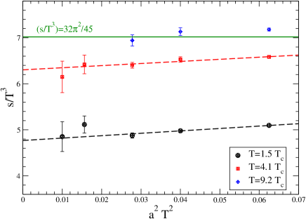
Figure 1: Scaling behavior of $s/T^{3}$, see Eq. (24). The Stefan-Boltzmann value is also displayed.

I thank Harvey B. Meyer for the intense and productive collaboration over the last year which led to the results discussed here. Many thanks to the organizers of the conference for their work, and for giving us the possibility to discuss physics in such a wonderful place.

References

- [1] L. Levkova, these proceedings.
- [2] J. Engels, F. Karsch, H. Satz, I. Montvay, Nucl. Phys. B205 (1982) 545.
- [3] J. Engels, J. Fingberg, F. Karsch, D. Miller, M. Weber, Phys. Lett. B252 (1990) 625-630.
- [4] G. Endrodi, Z. Fodor, S. D. Katz, K. K. Szabo, PoS LAT2007 (2007) 228, [arXiv:0710.4197].
- [5] H. B. Meyer, Phys. Rev. D80 (2009) 051502, [arXiv:0905.4229].
- [6] L. Giusti, H. B. Meyer, Phys. Rev. Lett. 106 (2011) 131601, [arXiv:1011.2727].
- [7] L. Giusti, H. B. Meyer, [arXiv:1110.3136].
- [8] M. Della Morte, L. Giusti, Comput. Phys. Commun. 180 (2009) 819-826, [arXiv:0806.2601].
- [9] M. Della Morte, L. Giusti, JHEP 1105 (2011) 056, [arXiv:1012.2562].
- [10] S. Necco, R. Sommer, Nucl. Phys. B622 (2002) 328-346. [hep-lat/0108008].
- [11] G. Boyd at al., Nucl. Phys. B469 (1996) 419-444, [hep-lat/9602007].
- [12] Y. Namekawa et al. [ CP-PACS Collaboration ], Phys. Rev. D64 (2001) 074507, [hep-lat/0105012].