Particle Counting Statistics of Time and Space Dependent Fields

Abstract

The counting statistics give insight into the properties of quantum states of light and other quantum states of matter such as ultracold atoms or electrons. The theoretical description of photon counting was derived in the 1960s and was extended to massive particles more recently. Typically, the interaction between each particle and the detector is assumed to be limited to short time intervals, and the probability of counting particles in one interval is independent of the measurements in previous intervals. There has been some effort to describe particle counting as a continuous measurement, where the detector and the field to be counted interact continuously. However, no general formula applicable to any time and space dependent field has been derived so far. In our work, we derive a fully time and space dependent description of the counting process for linear quantum many-body systems, taking into account the back-action of the detector on the field. We apply our formalism to an expanding Bose-Einstein condensate of ultracold atoms, and show that it describes the process correctly, whereas the standard approach gives unphysical results in some limits. The example illustrates that in certain situations, the back-action of the detector cannot be neglected and has to be included in the description.

I Introduction

The counting statistics of photons have been used to identify the quantum state of light since the beginnings of quantum optics. Despite early attempts Mandel (1958, 1959, 1963) to use a semiclassical approach, the theoretical description of the counting process requires a full quantum mechanical description of the electromagnetical field and the photocounter. This task was first achieved by Glauber Glauber (1963a, b, c, 1965), for an analogous approach see Kelley and Kleiner (1964), and will be referred to as the quantum counting formalism in the following. The formalism uses a full quantum mechanical description of the interaction between the incoming light and the atoms in the detector. However, consecutive detection events are treated independently, such that the effect of absorption of photons at the detector is neglected.

Even though the quantum counting formalism is being applied in a wide range of situations, its limits have been pointed out and discussed in the last decades. For example, for long detection times, it may lead to negative probabilities or expectation values exceeding the total number of photons. Such limitations were first pointed out by Mollow Mollow (1968) and several authors derived a formula taking into account the back-action of the detector on the field by considering the evolution of the system composed of the detector and the field Mollow (1968); Scully and W. E. Lamb (1969); Selloni et al. (1978). In 1981, Srinivas and Davies Srinivas and Davies (1981) provide a systematic description of photon counting as a continuous measurement process, where the detector continuously interacts with the light field. They derive their formalism based on a one-count operator and a no-count operator that determine the time evolution of the combined system of the detector and the light field. Whereas these operators are postulated in the model by Srinivas and Davies (SD model), Imoto and coworkers derived a microscopic theory of the continuous measurement of the photon number Imoto et al. (1990). They derive the no-count and one-count operators taking into account the interaction of the photons with the detector using the Jaynes-Cumming Hamiltonian for the field of a two-level atom. Photon counting including the back action of the detector has also been treated in Dodonov et al. (2007); Häyrynen et al. (2010).

Contrary to the quantum counting formalism, the SD model predicts that a substraction of one photon from a thermal state can increase the expectation value of the number of photons Ueda et al. (1990). Recently, this has been confirmed in an experiment where the action of the annihilation operator on different states of light has been implemented and measured Parigi et al. (2007). As discussed in Häyrynen et al. (2009) this is an experimental confirmation of the SD model.

The previous discussion suggests, that the SD model is a valid description for the photon counting process based on continuous measurements. However, a closed formula is derived only for the case of a single-mode field and the application of the formula to real experimental situation is therefore limited Mandel (1981); Fleischhauer and Welsch (1991). In 1987, Chmara derived a general formula for the photon counting distribution for a multimode field Chmara (1987) by applying the photon counting approach by SD to an open system. While the formula is in principle applicable to a wide class of systems, to our knowledge, no practical case where the time dependent intensities have been calculated has been reported.

In our work, we study the role of the back-action of the detector when counting massive particles, however, the results are valid also for photons. Previously we have shown that the particle counting statistics can be used as a detection method for many-body systems of ultracold atoms Braungardt et al. (2008, 2011a, 2011b). In this work we derive a general formula that describes the counting process including the back-action of the detector on the field. In contrast to the earlier descriptions of the counting process stated above, we give a fully time- and space dependent description of the process. We illustrate the importance of the back-action of the detector on the field by applying our formula to the detection of an expanding Bose Einstein condensate (BEC) by particle counting. We compare our formalism to the quantum counting formalism and to an approximate solution obtained by the Born approximation. We show that the approximate solutions, although more accurate than the quantum counting formalism, still fail to describe the counting process correctly.

The paper is organized as follows: In section II we review the quantum counting formalism and the SD model. In section III we consider a fully time- and space dependent description of the counting process and derive a formula for the counting distribution which is extended for two detectors in Sect. IV. We illustrate the space and time dependent counting process by considering the counting statistics of a freely expanding Bose Einstein condensate in Sect. V. We compare our time- and space-dependent counting formalism to the quantum counting formalism and show that it some limits, the last one leads to a divergent intensity at the detector. We also analyze the effect of the absorptive part in the modified field operator by comparing the exact solution to other approximative methods. We summarize our results in Sect.VI.

II Photon Counting: Standard approach and continuous measurement approach

In this section, we review the two main approaches to photon counting: The quantum counting formalism derived in the works of Glauber Glauber (1963a, b, c, 1965) and the continuous measurement approach derived by Srinivas and Davies Srinivas and Davies (1981).

II.1 The Quantum Counting Formalism

The derivation of the quantum counting formalism is based on the description of the quantum mechanical interaction of the photons with the atoms in the detector. The approach uses perturbation theory to describe the interaction for short intervals of time. The counting distribution for the full detection time $\tau$ is obtained by dividing it into small subintervals $\Delta\tau$ and treating the measurement in the full interval as a number of successive independent measurements in each interval. The approach thus describes a sequence of measurements, where the field evolves as in the absence of the detector. The method is based on the assumption, that the detection in one subinterval is independent of the detection in the previous subintervals. For the case of a light beam falling on a photo detector, it is argued (Mandel and Wolf, 1995, p. 723) that each element of the optical field interacts with the detector only briefly. The response time of the detector is short and the energy of the electron state is well defined after an interaction time $\Delta\tau$. For such a system where the unabsorbed photons escape, there is no need to consider the measurement back-action. The resulting equation for the counting distribution reads

$$p(m,t,\tau)=\langle\mathcal{T}:\frac{(\mathcal{I}(t))^{m}e^{-\mathcal{I}(t)}}{m!}:\rangle.$$ (1)

Here $\mathcal{T}$ and $::$ stand for time and normal ordering, respectively. The intensity operator $\mathcal{I}(t)$ is defined in terms of the positive and negative frequency parts $\hat{E}^{\pm}(\textbf{r},t)$ of the field operators by $\mathcal{I}(t)=\epsilon\int_{t}^{t+\tau}dt^{\prime}\int_{\Omega}\hat{E}^{-}(\textbf{r},t)\hat{E}^{+}(\textbf{r},t)d\textbf{r}$, where the spatial integral runs over the detector area $\Omega$ and $\epsilon$ denotes the efficiency of the detector. The normal ordering reflects the fact that the photons are annihilated at the detector. For a single mode field, the formula reads

$$p(m,\tau)=\sum_{n=m}^{\infty}\binom{n}{m}(\epsilon\tau)^{m}(\exp(-\epsilon\tau))^{n-m}\langle n|\rho|n\rangle.$$ (2)

where $\rho$ is the density matrix of the measured system.

II.2 The Back-action of the Detector on the Field

In Srinivas and Davies (1981) Srinivas and Davies developed an approach to photon counting based on continuous measurements over an extended period of time. Their work was motivated by the fact that the quantum counting formula Eq. (1) exhibits inconsistencies in the limit of long detection times, such as negative probabilities or mean particle numbers that exceed the total number of particles. For a single mode field the counting probability distribution is given by

$$p(m,t,\tau)=\sum_{n=m}^{\infty}\binom{n}{m}(1-e^{-\epsilon\tau})^{m}(\exp(-\epsilon\tau))^{n-m}\langle n|\rho|n\rangle.$$ (3)

This expression is formally equivalent to the quantum counting formula Eq. (2) with the term $\epsilon\tau$ substituted by $1-e^{-\epsilon\tau}$. For $\epsilon\tau\ll 1$, the two formulas are equivalent but the SD counting distribution in Eq. (3) does not suffer from the inconsistencies as the quantum counting formalism. The mean number of photons that are registered is bounded for $\tau\rightarrow\infty$ and no negative probabilities occur. However, the applicability of the formalism derived by Srinivas and Davies is limited to a one-mode field and therefore fails to describe most experimental situations.

Summarizing, the quantum counting formalism Eq.(2) becomes meaningless if $\epsilon\tau\gg 1$, when it can result in negative probabilities or unlimited mean number of counted photons as $\tau$ tends to infinity. Most experimentally relevant situations of photon counting are not in this limit and thus are well described by the quantum counting formalism. In our work we are interested in the counting statistics of many-body systems of cold atoms where one can control the space and time dependence. In the following section, we derive a formula for the counting distribution that takes into account the back-action of the detector on the field. It generalizes the formalism developed by Srinivas and Davies to time- and space dependent fields.

III Particle Counting of Time and Space Dependent Fields

The time- and space-dependent counting process can be described by a master equation that describes the interaction between the detector and the detected field $\Psi(\textbf{r},t)$. In typical experimental situations, the interaction between the detector and the field is restricted to a given volume, such as the surface of a photodetector or a microchannel plate. We define the function $\Omega(\textbf{r})$ to describe the spatial configuration of the detector. The master equation then reads

$$\dot{\rho}(t)=\epsilon\int d\textbf{r}\Omega(\textbf{r})\Psi(\textbf{r},t)\rho\Psi^{\dagger}(\textbf{r},t)$$

$$-\frac{\epsilon}{2}\int d\textbf{r}\Omega(\textbf{r})[\Psi(\textbf{r},t)^{\dagger}\Psi(\textbf{r},t)\rho-\rho\Psi(\textbf{r},t)^{\dagger}\Psi(\textbf{r},t)],$$ (4)

where $\rho(\textbf{r},t)$ denotes the density matrix of the system. The first term on the right-hand side of eq. (4) corresponds to the number of quantum jumps in the detector volume whereas the second term represents the damping of the field due to the absorption at the detector.
In order to solve the master equation (4) we first perform the transformation $\rho(t)=F(t)\tilde{\rho}(t)F^{\dagger}(t)$ and define

$$\tilde{\Psi}(\textbf{r},t)=F^{-1}(t)\Psi(\textbf{r},t)F(t),$$ (5)

where the operator $F(t)$ is defined as

$$F(t)=\mathcal{T}e^{-\epsilon/2\int_{0}^{t}dt^{\prime}\int d\textbf{r}^{\prime}\Omega(\textbf{r}^{\prime})\Psi^{\dagger}(\textbf{r}^{\prime},t^{\prime})\Psi(\textbf{r}^{\prime},t^{\prime})}.$$ (6)

Here, the term $\mathcal{T}$ on the left side of the operator denotes time ordering, whereas it denotes opposite time ordering on the right side of the operator. We use the relation $e^{\gamma A}Be^{-\gamma A}=B+\gamma[A,B]+\frac{\gamma^{2}}{2!}[A,[A,B]]+...$ and the commutation relations for linear fields, $[\Psi(\textbf{r},t),\Psi^{\dagger}(\textbf{r}^{\prime},t)]=\delta(\textbf{r},\textbf{r}^{\prime})$, $[\Psi(\textbf{r},t),\Psi^{\dagger}(\textbf{r}^{\prime},t^{\prime})]=G_{0}(\textbf{r},\textbf{r}^{\prime}|t,t^{\prime})$, $[\Psi(\textbf{r},t),\Psi(\textbf{r}^{\prime},t^{\prime})]=0$, where $G_{0}({\textbf{r}},{\textbf{r}^{\prime}}|t,t^{\prime})=\langle\textbf{r}|e^{-i(t-t^{\prime})/\hbar H_{0}}|\textbf{r}^{\prime}\rangle$ is the propagator for the time evolution for the Hamiltonian $H_{0}$ that describes the evolution of the field without detection.

The evolution of the rotated density matrix fulfills the equation

$$\dot{\tilde{\rho}}(\textbf{r},t)=\epsilon\int d\textbf{r}^{\prime}\Omega(\textbf{r}^{\prime})\tilde{\Psi}(\textbf{r},t)\tilde{\rho}\tilde{\Psi}^{\dagger}(\textbf{r},t).$$ (7)

A master equation of this kind, for non-rotated $\Psi$ and $\rho$ instead of $\tilde{\Psi}$ and $\tilde{\rho}$ leads to the quantum counting formalism described by eq. (1). Eq. (7) can be solved using perturbation theory (note that $\tilde{\rho}(0)=\rho(0))$, such that

$$\tilde{\rho}(t)=\rho(0)+\epsilon\int_{0}^{t}dt^{\prime}\int d\textbf{r}^{\prime}\Omega(\textbf{r}^{\prime})\tilde{\Psi}(\textbf{r}^{\prime},t^{\prime})\rho(0)\tilde{\Psi}^{\dagger}(x^{\prime},t^{\prime})$$ (8)

$$+\epsilon^{2}\int_{0}^{t}dt^{\prime}\int_{0}^{t^{\prime}}dt^{\prime\prime}\int d\textbf{r}^{\prime}\int d\textbf{r}^{\prime\prime}\Omega(\textbf{r}^{\prime})\Omega(\textbf{r}^{\prime\prime})\tilde{\Psi}(x^{\prime},t^{\prime})\tilde{\Psi}(x^{\prime\prime},t^{\prime\prime})\rho(0)\tilde{\Psi}^{\dagger}(x^{\prime\prime},t^{\prime\prime})\tilde{\Psi}^{\dagger}(x^{\prime},t^{\prime})+...$$

We use the cyclic properties of the trace to calculate the probability $p(m,\tau)$ of finding $m$ particles within the detector opening time $\tau$ and from the $m$th order term in the expansion in eq. III we get

$$p(m,\tau)=\langle\epsilon^{m}\int_{0}^{\tau}dt^{\prime}\int_{0}^{t^{\prime}}dt^{\prime\prime}..\int d\textbf{r}^{\prime}\int d\textbf{r}^{\prime\prime}\Omega(\textbf{r}^{\prime})\Omega(\textbf{r}^{\prime\prime})..$$ (9)

$$\tilde{\Psi}^{\dagger}(x^{\prime},t^{\prime})\tilde{\Psi}^{\dagger}(x^{\prime\prime},t^{\prime\prime})..F^{\dagger}(\tau)F(\tau)..\tilde{\Psi}(x^{\prime\prime},t^{\prime\prime})\tilde{\Psi}(x^{\prime\prime},t^{\prime})\rangle.$$

We rewrite this expression as a normal ordered expression with respect to the modified operators $\tilde{\Psi}$, which is also normal ordered with respect to the operators $\Psi$, as they are related by a linear transformation. Taking into account the normalization of the counting distribution, we obtain

$$p(m,\tau)=\langle\mathcal{T}:\frac{(\mathcal{I}(\tau))^{m}}{m!}e^{-\mathcal{I}(\tau)}:\rangle,$$ (10)

where the intensity at the detector is given by

$$\mathcal{I}(\tau)=\epsilon\int_{0}^{\tau}dt\int d\textbf{r}\Omega(\textbf{r})\tilde{\Psi}^{\dagger}(\textbf{r},t)\tilde{\Psi}(\textbf{r},t).$$ (11)

This equation is formally equivalent to the quantum counting formula, Eq. (1). However, whereas for the quantum counting formalism the intensity of particles registered at the detector is determined by the square of the field operator, in Eq. (25) the intensity is calculated using a modified field operator $\tilde{\Psi}(\textbf{r},t)$, which includes the absorption at the detector. In the following, we analyze these modified field operators.

We rewrite eq. (5) by dividing the detection time into small sub-intervals $\Delta t=t/N$. The time integration in Eq. (6) can be written as a sum, such that $F(t)=\prod_{i}F_{i}(t_{i})$, with $F_{i}(t_{i})=e^{-\frac{\epsilon}{2}\Delta t\int d\textbf{r}^{\prime}\Omega(\textbf{r}^{\prime})\Psi^{\dagger}(\textbf{r}^{\prime},t_{i})\Psi(\textbf{r}^{\prime},t_{i})}$, and we get

$$\tilde{\Psi}(\textbf{r},t)=F^{-1}_{1}(t_{1})...F_{N}^{-1}(t_{N})\Psi(\textbf{r},t)F_{N}(t_{N})...F_{1}(t_{1}).$$ (12)

We evaluate the expressions by using the commutation relations stated above. We start with the inner term,

$$F_{N}^{-1}(t_{N})\Psi(\textbf{r},t)F_{N}(t_{N})=e^{-\epsilon\Delta t\Omega(\textbf{r})}\Psi(\textbf{r},t_{N}).$$ (13)

The second term thus reads

$$e^{-\epsilon\Delta t\Omega(\textbf{r})}F_{N-1}^{-1}(t_{N-1})\Psi(\textbf{r},t_{N})F_{N-1}(t_{N-1})=$$

$$e^{-{\epsilon}\Delta t\Omega(\textbf{r})}\int d\textbf{r}^{\prime}e^{-{\epsilon}\Delta t\Omega(\textbf{r}^{\prime})}G_{0}(\textbf{r},\textbf{r}^{\prime},t_{N}-t_{N-1})\Psi(\textbf{r}^{\prime},t_{N-1})$$ (14)

The successive terms are calculated analogously, and in the limit of infinitesimal small time intervals we get

$$\tilde{\Psi}(\textbf{r},t)=\int d\textbf{r}^{\prime}G(\textbf{r},\textbf{r}^{\prime},t,t_{0})\Psi(\textbf{r}^{\prime},t_{0}),$$ (15)

where

$$G(\textbf{r},\textbf{r}^{\prime},t,t_{0})=\langle\textbf{r}|e^{-i(t-t_{0})/\hbar(\hat{H}_{0}-i{\epsilon}\hbar\hat{\Omega})}|\textbf{r}^{\prime}\rangle.$$ (16)

We have thus obtained an expression for the modified field operators $\tilde{\Psi}(\textbf{r},t)$ which differs from the definition of the standard field operator as it includes the propagation in an imaginary potential created by the detector. Together with the counting formula Eq. (10), this allows us, in principle, to calculate the counting distribution for time dependent systems with arbitrary detector geometries. However, solving Eq. (15) is in general a highly non-trivial task. In Sect. V we solve the equation for the detection of an expanding BEC.

It is interesting to point out that in many experimental situations, the detection process is fast compared to the time evolution of the system. In this case, we can neglect the part corresponding to the Hamiltonian $H_{0}$ in eq. (15) and get

$$\tilde{\Psi}(\textbf{r},t)=\int d\textbf{r}^{\prime}\langle\textbf{r}|e^{-{\epsilon}\hat{\Omega}(t-t_{0})}|\textbf{r}^{\prime}\rangle\Psi(\textbf{r}^{\prime},t_{0})$$

$$=e^{-{\epsilon}\hat{\Omega}(t-t_{0})}\Psi(\textbf{r},t_{0}).$$ (17)

The intensity (25) thus reads

$$\mathcal{I}(\tau)=\epsilon\int d\textbf{r}(1-e^{-\epsilon\Omega(\textbf{r})\tau})\Psi^{\dagger}(\textbf{r},t_{0})\Psi(\textbf{r},t_{0}),$$ (18)

which is a generalization of the formula Eq. (3) considering finite detector volumes. For $\epsilon\tau\ll 1$, Eq. (18) reduces to the quantum counting formula Eq. (1) for time independent systems.

IV Detection with Two Detectors

Our formalism is easily extended to calculate the joint counting probability for the detection at two detectors. The master equation that describes counting with two detectors reads

$$\dot{\rho}(t)=\epsilon_{1}\int d\textbf{r}\Omega_{1}(\textbf{r})\Psi(\textbf{r},t)\rho\Psi^{\dagger}(\textbf{r},t)$$

$$+\epsilon_{2}\int d\textbf{r}\Omega_{2}(\textbf{r})\Psi(\textbf{r},t)\rho\Psi^{\dagger}(\textbf{r},t)$$

$$-\frac{\epsilon_{1}}{2}\int d\textbf{r}\Omega_{1}(\textbf{r})(\Psi(\textbf{r},t)^{\dagger}\Psi(\textbf{r},t)\rho-\rho\Psi(\textbf{r},t)^{\dagger}\Psi(\textbf{r},t))$$

$$-\frac{\epsilon_{2}}{2}\int d\textbf{r}\Omega_{2}(\textbf{r})(\Psi(\textbf{r},t)^{\dagger}\Psi(\textbf{r},t)\rho-\rho\Psi(\textbf{r},t)^{\dagger}\Psi(\textbf{r},t)),$$ (19)

Similarly to the case of one detector described in Sect. III, we solve the master equation eq. (19) by performing the transformation $\rho(t)=F_{2}(t)\tilde{\rho}(t)F_{2}^{\dagger}(t)$ and

$$\tilde{\Psi}(\textbf{r},t)=F_{2}^{-1}(t)\Psi(\textbf{r},t)F_{2}(t),$$ (20)

where the operator $F_{2}(t)$ is defined as

$$F_{2}(t)=\mathcal{T}e^{-\epsilon_{1}/2\int_{0}^{t}dt^{\prime}\int d\textbf{r}^{\prime}\Omega_{1}(\textbf{r}^{\prime})\Psi^{\dagger}(\textbf{r}^{\prime},t^{\prime})\Psi(\textbf{r}^{\prime},t^{\prime})-\epsilon_{2}/2\int_{0}^{t}dt^{\prime}\int d\textbf{r}^{\prime}\Omega_{2}(\textbf{r}^{\prime})\Psi^{\dagger}(\textbf{r}^{\prime},t^{\prime})\Psi(\textbf{r}^{\prime},t^{\prime})}.$$ (21)

The evolution of the rotated density matrix is thus given by

$$\dot{\tilde{\rho}}(\textbf{r},t)=\epsilon_{1}\int d\textbf{r}^{\prime}\Omega_{1}(\textbf{r}^{\prime})\tilde{\Psi}(\textbf{r},t)\tilde{\rho}\tilde{\Psi}^{\dagger}(\textbf{r},t)$$

$$+\epsilon_{2}\int d\textbf{r}^{\prime}\Omega_{2}(\textbf{r}^{\prime})\tilde{\Psi}(\textbf{r},t)\tilde{\rho}\tilde{\Psi}^{\dagger}(\textbf{r},t),$$ (22)

The equation can be solved using perturbation theory, where we get an expression as in eq. (III) that includes correlation terms between the two detectors.

The conditional probability distribution of counting $m$ particles in one detector and $n$ particles in the other one thus reads

$$p(m,n)=\frac{(-1)^{m+n}}{m!n!}\frac{d^{m+n}}{d\lambda_{1}^{m}d\lambda_{2}^{n}}\mathcal{Q}\Big{|}_{\lambda_{1}=1,\lambda_{2}=1},$$ (23)

where

$$\mathcal{Q}(\lambda_{1},\lambda_{2})=\mbox{Tr}(\rho\mathcal{T}:e^{-\lambda_{1}\mathcal{I}_{1}-\lambda_{2}\mathcal{I}_{2}}:),$$ (24)

and

$$\mathcal{I}_{i}(\tau)=\epsilon_{i}\int_{0}^{\tau}dt\int d\textbf{r}\Omega_{i}(\textbf{r})\tilde{\Psi}^{\dagger}(\textbf{r},t)\tilde{\Psi}(\textbf{r},t).$$ (25)

The modified field operator that includes the absorption at the two detectors is given by

$$\tilde{\Psi}(\textbf{r},t)=\int d\textbf{r}^{\prime}\langle\textbf{r}|e^{-i(t-t_{0})/\hbar(\hat{H}_{0}-i\epsilon\hbar(\hat{\Omega}_{1}+\hat{\Omega}_{2}))}|\textbf{r}^{\prime}\rangle\Psi(\textbf{r}^{\prime},t_{0}).$$ (26)

V Detection of an Expanding Bose-Einstein Condensate

Let us now illustrate the space and time dependent counting process by considering the counting statistics of a freely expanding Bose Einstein condensate. For simplicity, we consider a one dimensional system with a point-like detector located at a distance $z_{0}$ from the condensate. The detection time is of the order of the system dynamics, such that we calculate the full time- and space dependent generating function with the intensity given by eq. (25). We consider a point-like detector placed at a distance $z_{0}$ from the center of the cloud. The detector is modeled by a delta-function $\delta(z-z_{0})$, such that the intensity eq. (25) reads

$$\mathcal{I}=\epsilon\int_{0}^{t}dt^{\prime}\tilde{\Psi}^{\dagger}(z_{0},t^{\prime})\tilde{\Psi}(z_{0},t^{\prime}),$$ (27)

where the time evolution of the operators $\tilde{\Psi}(\textbf{r},t)$ is described by eq. (15). For the detection of a 1D BEC at a point-like detector, the time evolution of the single-particle wave function is given by

$$\tilde{\phi}(z,t)=\int dz^{\prime}G(z,z^{\prime},t,t_{0})\phi(z^{\prime},t_{0}),$$ (28)

where

$$G(z,z^{\prime},t,t_{0})=\langle z|e^{-i(t-t_{0})/\hbar(\hat{H}_{0}-i\hbar\epsilon\hat{\delta})}|z^{\prime}\rangle$$ (29)

The counting distribution is then obtained from eq. (10), which for the case of a condensate with $N$ particles reads

$$p(m)=\frac{\left(N\epsilon\int dt\tilde{\phi}^{\dagger}(z_{0},t)\tilde{\phi}(z_{0},t)\right)^{m}}{m!}e^{-N\epsilon\int dt\tilde{\phi}^{\dagger}(z_{0},t)\tilde{\phi}(z_{0},t)},$$ (30)

In the following subsection, we exactly solve eq. (28), where we approximate the initial wave function $\tilde{\phi}(z,0)$ by a Lorentzian function,

$$\tilde{\phi}(z,0)=\sqrt{\Gamma}e^{-\Gamma|z|}.$$ (31)

In Subsect. V.2, we calculate an approximate solution obtained by the Born approximation. In Subsect. V.3 we compare the exact solution to the approximate solution as well as to the quantum counting formalism.

V.1 Exact solution

We calculate the counting distribution $p(m)$ for an expanding BEC, where the detector is located at some distance $z_{0}$ from the center of the cloud. We follow the treatment in Kleber (1994) to derive an exact solution for the propagator eq. (29) that describes the whole system evolution including the absorption at the detector. The system Hamiltonian is composed of two parts: the free particle Hamiltonian $H_{0}$ and a part corresponding to the detection process, which acts as an imaginary potential. The propagator $G(z,z^{\prime},t)$ that describes the time evolution of the wave-function including the absorption at the detector can be written in an iterative way using the Lippmann-Schwinger equation, which for a point-like detector $\Omega(z^{\prime})=\delta(z^{\prime}-z_{0})$ reads

$$G(z,z^{\prime},t)=G_{0}(z,z^{\prime},t)-$$

$$\frac{\epsilon}{\hbar}\int_{0}^{t}dt^{\prime}G_{0}(z,z_{0},t-t^{\prime})G(z_{0},z^{\prime},t^{\prime}).$$ (32)

In the Appendix, we solve the Lippmann-Schwinger equation and show that the full propagator that describes the back-action of the detector is given by

$$G(z_{0},z^{\prime},t)=G_{0}(z_{0},z^{\prime}t)$$

$$+\frac{im\epsilon}{\hbar}M(|z-z_{0}|+|z^{\prime}-z_{0}|,-\frac{m\epsilon}{\hbar},\frac{\hbar}{m}t),$$ (33)

where $M(z,k,t)$ denotes the Moshinsky function Kramer and Moshinsky (2005)

$$M(z,k,t)=\int_{-\infty}^{0}dz^{\prime}\frac{1}{\sqrt{2\pi it}}\exp\left(ikz^{\prime}+i\frac{(z-z^{\prime})^{2}}{2t}\right)$$

$$=\frac{1}{2}\exp\left(ikz-i\frac{1}{2}k^{2}t\right)\hbox{erfc}(e^{-i\pi/4}\frac{z-kt}{\sqrt{2t}})$$ (34)

The modified wave function $\tilde{\phi}(z_{0},t)$ can then be calculated by standard integration techniques using eq. (28), and the counting distribution $p(m)$ obtained by eq. (30). The counting statistics are determined by the time integral over the square of the wave function $\tilde{\phi}(z_{0},t)$. Fig. 1 a shows the square of the wave function with respect to time for different distances $z_{0}$. As the distance increases, the wave function spreads in time. In order to obtain non-trivial results, long opening times are required. Fig. 1 b shows the intensity of particles at the detector with respect to the opening time $\tau$ for detectors placed at different distances from the detector.

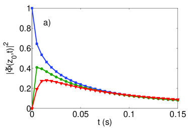
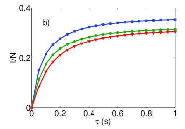
Figure 1: Density $|\tilde{\phi}(z_{0},t)|^{2}$ with respect to time (Fig a) and normalized intensity $\mathcal{I}/N$ with respect to $\tau$ (Fig. b) for $z_{0}=0$ (blue squares), $z_{0}=0.1/\Gamma$ (green circles), $z_{0}=0.4/\Gamma$ (red diamonds). As the distance $z_{0}$ between the center of the cloud and the detector increases, the wave function spreads and long detector opening times are required to achieve non-trivial intensities. Parameters used: $z_{0}=0,\epsilon=1,N=100,\Gamma=10^{5}$.

V.2 Born Approximation

In the previous section, we obtained an exact solution for the time evolution of the wavefunction by solving the Lippmann-Schwinger equation (32). In this section, we use the Born approximation in order to derive an expression for $\tilde{\phi}(z,t)$ in terms of the known propagator $G_{0}$. In the second order approximation, we obtain

$$G(z,z^{\prime},t)=G_{0}(z,z^{\prime},t)-\frac{\epsilon}{\hbar}\int_{0}^{t}dt^{\prime}G_{0}(z,z_{0},t-t^{\prime})G_{0}(z_{0},z^{\prime},t^{\prime}).$$ (35)

This implies that up to second order, the solution to eq. (28) is given by

$$\tilde{\phi}(z,t)=\phi(z,t)$$

$$-\frac{\epsilon}{\hbar}\int_{0}^{t}dt^{\prime}\int dz^{\prime}G_{0}(z,z_{0},t-t^{\prime})G_{0}(z_{0},z^{\prime},t^{\prime})\phi(z^{\prime},t_{0}).$$

$$=2\sqrt{\Gamma}(M(z_{0},-i\Gamma,\hbar t/m)-$$

$$\frac{\epsilon}{\hbar}\int_{0}^{t}dt^{\prime}\sqrt{\frac{m}{2\pi\hbar it^{\prime}}}M(z_{0},-i\Gamma,\hbar t^{\prime}/m))$$ (36)

Eq. (36) describes the evolution of the wave function, where the absorption at the detector is taken into account up to second order. We get the higher order Born approximation by writing eq. (36) in exponential form,

$$\tilde{\phi}(\textbf{z},t)=\sqrt{\Gamma}M(z_{0},-i\Gamma,\hbar t/m)\times$$

$$e^{-\epsilon/\hbar\int_{0}^{t}dt^{\prime}\sqrt{\frac{m}{2\pi\hbar it^{\prime}}}M(z_{0},-i\Gamma,\hbar t^{\prime}/m)/M(z_{0},-i\Gamma,\hbar t/m)}$$ (37)

In Sect. V.3, we show that the Born approximation describes the situation more accurately than the quantum counting formalism. However, the effect of the absorption is under-estimated.

V.3 Effect of the Absorption at the Detector

Let us now analyze the effect of the back-action of the detector on the field. From eq. (30) it is clear that the important quantities to study are the square of the wave function, $\tilde{\phi}^{*}(z_{0},t)\tilde{\phi}(z_{0},t)$, its time integral, as well as the full counting distribution. We discuss the limits in which the quantum counting formalism and the Born approximation give valid results, and study the limitations of the approximative solutions.

In Fig. 2a, we plot the square of the wave function with respect to time, and compare the exact solution to the solutions obtained by the born approximation and the quantum counting formalism. The exact graph corresponding to the exact solution decays more rapidly, as the absorption at the detector is considered. The Born approximation underestimates the decay of the wave function and thus the absorption, however, it describes the behavior more accurately than the quantum counting formalism, where absorption is not considered.

The effect is seen more clearly when studying the intensity of the field at the detector, which is given by the time integral $\epsilon\int_{0}^{\tau}dt\tilde{\phi}^{*}(z_{0},t)\tilde{\phi}(z_{0},t)$ (Fig. 2b). For short detection times, the exact solution and the approximate solutions coincide. As the detection time increases, the intensity of particles is overestimated both for the Born approximation and for the quantum counting formalism. Note that for long detection times, the second order Born approximation diverges, whereas the exponential Born approximation reaches an asymptotic value.

Finally, we compare the counting distributions obtained by the exact solution eq. (28) to the solution obtained by the quantum counting formalism and the Born approximation. The effect of absorption is clearly visible in the counting distribution, where the approximate solutions deviate increasingly from the exact solution as the measurement time increases (Fig. 3). The counting distribution calculated with the full formalism including detection is clearly different from the approximated solution.

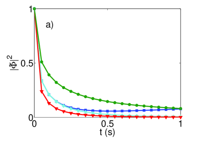
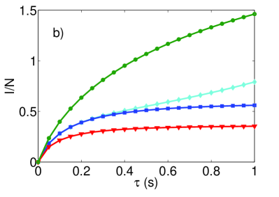
Figure 2: a) $|\tilde{\phi}(0,t)|^{2}$ with respect to $t$. b) Normalized intensity $\mathcal{I}/N$ with respect to $\tau$. We compare the exact solution (red triangles), second order Born approximation (blue squares), exponential Born approximation (light blue diamonds) and the quantum counting formalism (green circles). Both the quantum counting formalism and the Born approximation reach intensities that exceed the total number of particles for long opening times $\tau$. In the exponential Born approximation the intensity is bounded for large $\tau$, however, the asymptotic value exceeds the bound given by the exact solution. Parameters used: $z_{0}=0,\epsilon=1,N=100,\Gamma=10^{5}$.

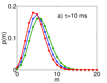
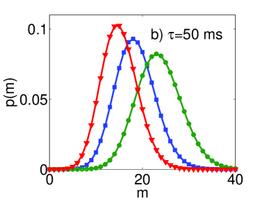
Figure 3: Counting distribution p(m) obtained from exact solution (red triangles), Born approximation (blue squares) and the quantum counting formalism (green circles). For short detection times (Fig. a) the approximations agree reasonably well with the exact solution. For longer detection times (Fig. b), the approximations are no longer valid. Parameters used: $z_{0}=0,\epsilon=1,N=100,\Gamma=10^{5}$.

VI Summary and Conclusions

We have derived a formalism for describing the counting distribution of space- and time dependent fields taking into account the back-action of the detector on the field. We have illustrated the importance of the effect of the back-action for the free expansion of a Bose Einstein condensate. An approximate solution using the Born approximation describes the behavior of the system more accurately than the quantum counting formalism. However, for typical detection times of expanding BECs, the effect of absorption is under-estimated significantly both by the quantum counting formalism, as well as the Born approximation. We thus showed that for certain experimentally relevant situations, the full time- and space dependent formalism has to be applied.

*

Appendix A Derivation of the Propagator Including the Back-action of the Detector

We solve the Lippmann-Schwinger equation for the propagator $G(z,z^{\prime},t)$ that describes the time evolution of the wave-function including the absorption at a point-like detector $\Omega(z^{\prime})=\delta(z^{\prime}-z_{0})$,

$$G(z,z^{\prime},t)=G_{0}(z,z^{\prime},t)-$$

$$\frac{\epsilon}{\hbar}\int_{0}^{t}dt^{\prime}G_{0}(z,z_{0},t-t^{\prime})G(z_{0},z^{\prime},t^{\prime}),$$ (38)

where the propagator $G_{0}(z,z^{\prime},t)$ for the free expansion is given by

$$G_{0}(z,z^{\prime},t)=\sqrt{\frac{m}{2\pi i\hbar t}}\exp(\frac{i|z-z^{\prime}|^{2}}{2\hbar t}).$$ (39)

We perform a Laplace transform of eq. (38) and use the convolution theorem to get

$$\tilde{G}(z,z^{\prime},s)=\tilde{G}_{0}(z,z^{\prime},t)-\frac{\epsilon}{\hbar}\tilde{G}_{0}(z,z_{0},s)\tilde{G}(z_{0},z^{\prime},s)$$ (40)

From eq. (27), we observe that we are only interested in the propagator at $z=z_{0}$, such that

$$\tilde{G}(z_{0},z^{\prime},s)=\frac{\tilde{G}_{0}(z_{0},z^{\prime},t)}{1-\frac{\epsilon}{\hbar}\tilde{G}_{0}(z_{0},z_{0},s)}.$$ (41)

The Laplace transform of the free propagator $G(z_{0},z^{\prime},s)$ is given by

$$\tilde{G}(z_{0},z^{\prime},s)=\sqrt{\frac{m}{2i\hbar s}}\exp(-\sqrt{\frac{2ms}{i\hbar}}|z_{0}-z^{\prime}|).$$ (42)

The inverse Laplace transform of $\tilde{G}(z,z^{\prime},s)$ can be performed by standard methods Abramowitz and Stegun [1965], such that the propagator is given by

$$G(z_{0},z^{\prime},t)=G_{0}(z_{0},z^{\prime}t)$$

$$+\frac{im\epsilon}{\hbar}M(|z-z_{0}|+|z^{\prime}-z_{0}|,-\frac{m\epsilon}{\hbar},\frac{\hbar}{m}t),$$ (43)

where $M(z,k,t)$ is defined in eq. (34). The function $\tilde{\phi}(z_{0},t)$ is then calculated by eq. (28).

Note that for a detector placed at $z_{0}=0$ in the center of the cloud, the counting formula can also be obtained by directly solving the time dependent Schrödinger equation,

$$i\hbar\dot{\tilde{\phi}}(z,t)=-\frac{\hbar^{2}}{2m}\frac{\partial^{2}}{\partial z^{2}}\tilde{\phi}(z,t)-i\hbar\epsilon\delta(z)\tilde{\phi}(z,t)$$ (44)

with the initial condition given by

$$\tilde{\phi}(z,0)=\sqrt{\Gamma}e^{-\Gamma|z|}.$$

In order to solve eq. (44), we first express it in terms of its fourier transform. From eq. (27) is is clear that for a detector placed at $z_{0}=0$, we are only interested in $\tilde{\phi}(0,t)=\frac{1}{\sqrt{2\pi\hbar}}\int_{-\infty}^{\infty}dk\phi(k,t)$. The fourier transformed equation is a differential equation with variable coefficients and can be integrated by standard methods Bronstein et al. [2002]. We get

$$\tilde{\phi}(0,t)=\tilde{\phi}_{0}(t)-\frac{\epsilon}{\sqrt{2\pi\hbar}}\int_{0}^{t}\kappa(t-t^{\prime})\tilde{\phi}(0,t^{\prime})dt^{\prime},$$ (45)

where $\tilde{\phi}_{0}(t)=\frac{1}{\sqrt{2\pi\hbar}}\int dke^{\frac{-ik^{2}t}{2\hbar m}}\phi(k,0)$ and $\kappa(t,t^{\prime})=\frac{1}{\sqrt{2\pi\hbar}}\int_{-\infty}^{\infty}dke^{\frac{-ik^{2}(t-t^{\prime})}{2\hbar m}}=\frac{(1-i)\sqrt{m}}{\sqrt{2(t-t^{\prime})}}$ We take the Laplace transform of eq. (45) and use the convolution theorem [Abramowitz and Stegun, 1965, 29.2.8] to obtain

$$\tilde{\phi}(0,s)=\frac{\tilde{\phi}_{0}(s)}{1+\frac{\epsilon}{\sqrt{2\pi\hbar}}\kappa(s)}.$$ (46)

The term $\tilde{\phi}_{0}(s)$ is calculated by using the residue theorem. Using the method of partial fractions the expression for $\tilde{\phi}(0,s)$ is written in the form $\frac{A}{\sqrt{s}+a_{1}}$, such that the inverse Laplace transform is given by

$$\tilde{\phi}(0,t)=\frac{\sqrt{\Gamma}(\hbar\Gamma e^{\frac{i\hbar\Gamma^{2}t}{2m}}\hbox{Erfc}(\frac{1+i}{2}\sqrt{\hbar t/m}\Gamma)+im\epsilon e^{-\frac{imt\epsilon^{2}}{2\hbar}}\hbox{Erfc}(\frac{1-i}{2}\epsilon\sqrt{tm/\hbar})}{(\hbar\Gamma+im\epsilon)}.$$ (47)

References

- Mandel [1958] L. Mandel. Fluctuations of photon beams and their correlations. Proc. Phys. Soc (London), 72:1037, 1958.
- Mandel [1959] L. Mandel. Fluctuations of photon beams - the distribution of the photo electrons. Proc. Phys. Soc (London), 74:233, 1959.
- Mandel [1963] L. Mandel. Fluctuations of light beams. in: Progress in Optics, page 181, 1963. ed. E. Wolf (North-Holland, Amsterdam).
- Glauber [1963a] R. J. Glauber. Photon correlations. Phys. Rev. Lett., 10:84, 1963a.
- Glauber [1963b] R. J. Glauber. Coherent and incoherent states of the radiation field. Phys. Rev., 131:2766–2788, 1963b.
- Glauber [1963c] R. J. Glauber. The quantum theory of optical coherence. Phys. Rev., 130:2529–2539, 1963c.
- Glauber [1965] R. J. Glauber. Optical coherence and photon statistics. page 65, New York, 1965. Gordon & Breach.
- Kelley and Kleiner [1964] P. L. Kelley and W. H. Kleiner. Theory of electromagnetic field measurement and photoelectron counting. Phys. Rev., 136(A316-A334), 1964.
- Mollow [1968] B. R. Mollow. Quantum theory of field attenuation. Phys. Rev., 168(1896), 1968.
- Scully and W. E. Lamb [1969] M. O. Scully and Jr. W. E. Lamb. Quantum theory of an optical maser. iii. theory of photoelectron counting statistics. Phys. Rev., 179(368), 1969.
- Selloni et al. [1978] A. Selloni, P. Schwendimann, P. Quattropani, and H. P. Baltes. Open system theory of photodetection: dynamics of field and atomic moments. J. Phys. A, 11(1427), 1978.
- Srinivas and Davies [1981] M. D. Srinivas and E. B. Davies. Photon counting probabilities in quantum optics. Opt. Acta, 28:981–996, 1981.
- Imoto et al. [1990] N. Imoto, M. Ueda, and T. Ogawa. Microscopic theory of continuous measurement of photon number. Phys. Rev. A, 41(7):4127–4129, 1990.
- Dodonov et al. [2007] A. V. Dodonov, S. S. Mizrahi, and V. V. Dodonov. Inclusion of nonidealities in the continuous photodetection. Phys. Rev. A, 75(013806), 2007.
- Häyrynen et al. [2010] T. Häyrynen, J. Oksanen, and J. Tulkki. Derivation of generalized quantum jump operators and comparison of the microscopic single photon detector models. Eur. Phys. J. D, 56:113–121, 2010.
- Ueda et al. [1990] M. Ueda, N. Imoto, and T. Ogawa. Quantum theory for continuous photodetection processes. Phys. Rev. A, 41(7):3891–3904, 1990.
- Parigi et al. [2007] V. Parigi, A. Zavatta, M. Kim, and M. Bellini. Probing quantum commutation rules by addition and subtraction of single photons to/from a light field. Science, 317(1890-1893), 2007.
- Häyrynen et al. [2009] T. Häyrynen, J. Oksanen, and J. Tulkki. Exact theory for photon subtraction for fields from quantum to classical limit. Eur. Phys. Lett., 78(44002), 2009.
- Mandel [1981] L. Mandel. Comment on ’photon counting probabilities in quantum optics’. Opt. Acta, 28:1447–1450, 1981.
- Fleischhauer and Welsch [1991] M. Fleischhauer and D. G. Welsch. Nonperturbative approach to multimode photodetection. Phys. Rev. A, 44(1):747–755, 1991.
- Chmara [1987] W. Chmara. A quantum open-systems theory approach to photodetection. J. Mod. Opt., 34(455-467), 1987.
- Braungardt et al. [2008] S. Braungardt, A. Sen, U. Sen, R. J. Glauber, and M. Lewenstein. Fermion and spin counting in strongly correlated systems. Phys. Rev. A, 78:063613, 2008.
- Braungardt et al. [2011a] S. Braungardt, M. Rodr guez, A. Sen(De), U. Sen, R. J. Glauber, and M. Lewenstein. Counting of fermions and spins in strongly correlated systems in and out of thermal equilibrium. Phys. Rev. A, 83:013601, 2011a.
- Braungardt et al. [2011b] S. Braungardt, M. Rodr guez, A. Sen(De), U. Sen, and M. Lewenstein. Atom counting in expanding ultracold clouds. arXiv:1103.1868v1 [quant-ph], 2011b.
- Mandel and Wolf [1995] L. Mandel and E. Wolf. Optical Coherence and quantum optics. Cambridge University Press, Cambridge, 1995.
- Kleber [1994] M. Kleber. Exact solutions for time-dependent phenomena in quantum mechanics. Physics Reports, 236:331–393, 1994.
- Abramowitz and Stegun [1965] M. Abramowitz and I.A. Stegun. Handbook of Mathematical Functions. Dover, New York, 1965.
- Kramer and Moshinsky [2005] T. Kramer and M. Moshinsky. Tunnelling out of a time-dependent well. J. Phys. A, 38:5993–6003, 2005.
- Bronstein et al. [2002] I. N. Bronstein, K. A. Semendjajew, G. Musiol, and H. Muehlig. Handbook of Mathematics. Springer, 2002.