Fourth-generation SM imprints in $B\to K^{\ast}\ell^{+}\ell^{-}$ decays with polarized $K^{\ast}$

Abstract

The implication of the fourth-generation quarks in the $B\to K^{\ast}\ell^{+}\ell^{-}$ ($\ell=\mu,\tau$) decays, when $K^{\ast}$ meson is longitudinally or transversely polarized, is presented. In this context, the dependence of the branching ratio with polarized $K^{\ast}$ and the helicity fractions ($f_{L,T}$) of $K^{\ast}$ meson are studied. It is observed that the polarized branching ratios as well as helicity fractions are sensitive to the NP parameters, especially when the final state leptons are tauons. Hence the measurements of these observables at LHC can serve as a good tool to investigate the indirect searches of new physics beyond the Standard Model.

I Introduction

It is well known that the Standard Model (SM) with single Higgs boson is the simplest one and has been tested with great precision. Despite its many successes it has some theoretical shortcomings which preclude to recognize the SM as a fundamental theory. For example the SM doesn’t addresses the following issues (i) hierarchy puzzle (ii) origin of mass spectrum (iii) Why only three generations of quarks and leptons? (iv) Neutrinos are massless but experiments have shown that the neutrinos have non-zero mass.

The above mentioned issues indicate that there must be a new physics (NP) beyond the SM. Various extensions of the SM are motivated to understand some of the above mentioned problems. These extensions are two Higgs doublet models (2HDM), minimal supersymmetric SM (MSSM), universal extra dimension model (UED) and Standard model with fourth generation (SM4)etc. SM4 implying a fourth family of quarks and leptons seems to most economical in number of additional particles and simpler in the sense that it does not introduce any new operators. Interest in SM4 was fairly high in the 1980s until the electroweak precision data seemed to rule it out. The other reason which increases the interest in the fourth generation was the measurement of the number of light neutrinos at the $Z$ pole that showed only three light neutrinos could exist. However, the discovery of neutrino oscillations suggested the possibility of a mass scale beyond the SM, and the models with the sufficiently massive neutrino became acceptable Pree . Though the early study of the EW precision measurements ruled out a fourth generation PDG , however it was subsequently pointed out Maltoni that if the fourth generation masses are not degenerate, then the EW precision data do not prohibit the fourth generation Kible . Therefore, the SM can be simply extended with a sequential as four quark and four lepton left handed doublets and corresponding right handed singlets.

The possible sequential fourth generation may play an important role in understanding the well known problem of CP violation and flavor structure of standard theory 3 ; 4 ; 5 ; 6 ; 7 ; 8 ; 9 , electroweak symmetry breaking 10 ; 11 ; 12 ; 13 , hierarchies of fermion mass and mixing angle in quark/lepton sectors 14 ; 15 ; 16 ; 17 ; 18 . A thorough discussion on the theoretical and experimental aspects of the fourth generation can be found in ref. 19 .

It is necessary to mention here that the SM4 particles are heavy in nature, consequently they are hard to produce in the accelerators. Therefore, we have to go for some alternate scenarios where we can find their influence at low energies. In this regard, the Flavor Changing Neutral Current (FCNC) transitions provide an ideal plateform to establish new physics (NP). This is because of the fact that FCNC transitions are not allowed at tree level in the SM and are allowed at loop level through GIM mechanism which can get contributions of NP from newly proposed particles via loop diagrams. Among different FCNC transitions the one $b\rightarrow s$ transition plays a pivotal role to perform efficient tests of NP scenarios 25 ; 26 ; 27 ; 28 ; 29 ; 30 ; 31 ; 32 ; 33 . It is also the fact that $CP$ violation in $b\rightarrow s$ transitions is predicted to be very small in the SM, thus, any experimental evidence for sizable $CP$ violating effects in the $B$ system would clearly point towards a NP scenario. The FCNC transitions in SM4 contains much fewer parameters and has a possibility of having simultaneously sizeable effects in $K$ and $B$ mesons system compared to other NP models.

The exploration of Physics beyond the Standard model through various inclusive $B$ meson decays like $B\to X_{s,d}\ell^{+}\ell^{-}$ and their corresponding exclusive processes, $B\to M\ell^{+}\ell^{-}$ with $M=K,K^{\ast},K_{1},\rho$ etc have been done in literature bst ; 63 ; zp ; colangelo ; pbr ; aqeel . These studies showed that the above mentioned inclusive and exclusive decays of $B$ meson are very sensitive to the flavor structure of the Standard Model and provide a windowpane for any NP model. There are two different ways to incorporate the NP effects in the rare decays, one through the modification in Wilson coefficients and the other through new operators which are absent in the Standard Model. It is necessary to mention here the FCNC decay modes like $B\to X_{s}\ell^{+}\ell^{-}$, $B\to K^{\ast}\ell^{+}\ell^{-}$ and $B\to K\ell^{+}\ell^{-}$ which are also useful in the determination of precise values of $C_{7}^{eff}$, $C_{9}^{eff}$ and $C_{10}^{eff}$ Wilson coefficients as well as the sign of $C_{7}^{eff}.$ In particular these decay modes involved observables which can distinguish between the various extensions of Standard Model.

The observables like branching ratio, forward-backward asymmetry,lepton polarization asymmetries and helicity fractions of final state mesons for the semileptonic $B$ decays are greatly influenced under different scenarios beyond the Standard Model. Therefore, the precise measurement of these observables will play an important role in the indirect searches of NP including SM4. In this work we study the physical observables such as branching ratio and helicity fractions when $K^{\ast}$ meson is longitudinally and transversely polarized for the decays $B\to K^{\ast}\ell^{+}\ell^{-}$ in SM4. The longitudinal helicity fraction $f_{L}$ has been measured for the $K^{\ast}$ meson by LHCbLHCb , CDFCDF ,Belle Belle and Babar babar collaborations for the decay channel $B\to K^{\ast}\mu^{+}\mu^{-}$. The recent results are quite intriguing especially that from LHCb and CDF collaborations. In this respect it is appropriate to look for the above mentioned observables which can be tested experimentally to pin down the status of SM4. In exclusive decays the main job is to calculate the form factors, for our analysis we borrow the light cone QCD sum rules form factors (LCSR)Ball .

We organize the manuscript as follows: In sec. II, we fill our toolbox with the theoretical framework needed to study the said process in the fourth-generation SM. In Sec. III, we discuss the phenomenology of the polarized branching ratios and helicity fractions of $K^{\ast}$ meson in $B\rightarrow K^{\ast}\ell^{+}\ell^{-}$ in detail. We give the numerical analysis of our observables and discuss the sensitivity of these observables with the NP scenarios. We summarize the main points of our findings in Sec. IV.

II Theoretical Toolbox

At quark level the decay $B\rightarrow K^{\ast}\ell^{+}\ell^{-}$ $(\ell=\mu,\tau)$ is governed by the transition $b\rightarrow s\ell^{+}\ell^{-}$ for which the effective Hamiltonian can be written as

$$H_{eff}=-\frac{4G_{F}}{\sqrt{2}}V_{tb}V^{\ast}_{ts}{\sum\limits_{i=1}^{10}}C_{i}({\mu})O_{i}({\mu}),$$ (1)

where $O_{i}({\mu})$ $(i=1,\ldots,10)$ are the four-quark operators and $C_{i}({\mu})$ are the corresponding Wilson coefficients at the energy scale ${\mu}$ and the explicit expressions of these in the SM at NLO and NNLO are given in Buchalla ; Buras ; Ball ; Ali ; Kim ; Kruger ; Grinstein ; Cella ; Bobeth ; Asatrian ; Misiak ; Huber . The operators responsible for $B\rightarrow K^{\ast}\ell^{+}\ell^{-}$ are $O_{7}$, $O_{9}$ and $O_{10}$ and their form is given by

$$O_{7} = \frac{e^{2}}{16\pi^{2}}m_{b}\left(\bar{s}\sigma_{\mu\nu}P_{R}b\right)F^{\mu\nu},\,$$

$$O_{9} = \frac{e^{2}}{16\pi^{2}}(\bar{s}\gamma_{\mu}P_{L}b)(\bar{l}\gamma^{\mu}l),\,$$ (2)

$$O_{10} = \frac{e^{2}}{16\pi^{2}}(\bar{s}\gamma_{\mu}P_{L}b)(\bar{l}\gamma^{\mu}\gamma_{5}l),$$

with $P_{L,R}=\left(1\mp\gamma_{5}\right)/2$.

In terms of the above Hamiltonian, the free quark decay amplitude for $b\rightarrow s$ $\ell^{+}\ell^{-}$ in SM4 can be derived as:

$$\mathcal{M}(b\rightarrow s\ell^{+}\ell^{-})=-\frac{G_{F}\alpha}{\sqrt{2}\pi}V_{tb}V_{ts}^{\ast}\bigg{\{}C_{9}^{eff}(\bar{s}\gamma_{\mu}Lb)(\bar{\ell}\gamma^{\mu}\ell)$$

$$+C_{10}(\bar{s}\gamma_{\mu}Lb)(\bar{\ell}\gamma^{\mu}\gamma_{5}\ell)-2m_{b}C_{7}^{eff}(\bar{s}i\sigma_{\mu\nu}\frac{q^{\nu}}{q^{2}}Rb)(\bar{\ell}\gamma^{\mu}\ell)\bigg{\}}$$ (3)

where $q^{2}$ is the square of momentum transfer. The operator $O_{10}$ can not be induced by the insertion of four-quark operators because of the absence of the $Z$-boson in the effective theory. Therefore, the Wilson coefficient $C_{10}$ does not renormalize under QCD corrections and hence it is independent on the energy scale. In addition to this, the above quark level decay amplitude can receive contributions from the matrix element of four-quark operators, $\sum_{i=1}^{6}\langle\ell^{+}\ell^{-}s|O_{i}|b\rangle$, which are usually absorbed into the effective Wilson coefficient $C_{9}^{SM}(\mu)$ and can usually be called $C_{9}^{eff}$, that can be found in Ball ; aqeel

The sequential fourth generation model with an additional up-type quark $t^{\prime}$ and down-type quark $b^{\prime}$ , a heavy charged lepton $\tau^{\prime}$ and an associated neutrino $\nu^{\prime}$ is a simple and non-supersymmetric extension of the SM, and as such does not add any new dynamics to the SM. Being a simple extension of the SM it retains all the properties of the SM where the new top quark $t^{\prime}$ like the other up-type quarks, contributes to $b\to s$ transition at the loop level. Therefore, the effect of fourth generation displays itself by changing the values of Wilson coefficients $C_{7}\left(\mu\right)$, $C_{9}\left(\mu\right)$ and $C_{10}$ via the virtual exchange of fourth generation up-type quark $t^{\prime}$ which then take the form;

$$\lambda_{t}C_{i}\rightarrow\lambda_{t}C_{i}^{SM}+\lambda_{t^{\prime}}C_{i}^{new},$$ (4)

where $\lambda_{f}=V_{fb}^{\ast}V_{fs}$ and the explicit forms of the $C_{i}$’s can be obtained from the corresponding expressions of the Wilson coefficients in the SM by substituting $m_{t}\rightarrow m_{t^{\prime}}$. By adding an extra family of quarks, the CKM matrix of the SM is extended by another row and column which now becomes $4\times 4$. The unitarity of which leads to

$$\lambda_{u}+\lambda_{c}+\lambda_{t}+\lambda_{t^{\prime}}=0.$$

Since $\lambda_{u}=V_{ub}^{\ast}V_{us}$ has a very small value compared to the others, therefore, we will ignore it. Then $\lambda_{t}\approx-\lambda_{c}-\lambda_{t^{\prime}}$ and from Eq. (4) we have

$$\lambda_{t}C_{i}^{SM}+\lambda_{t^{\prime}}C_{i}^{new}=-\lambda_{c}C_{i}^{SM}+\lambda_{t^{\prime}}\left(C_{i}^{new}-C_{i}^{SM}\right).$$ (5)

One can clearly see that under $\lambda_{t^{\prime}}\rightarrow 0$ or $m_{t^{\prime}}\rightarrow m_{t}$ the term $\lambda_{t^{\prime}}\left(C_{i}^{new}-C_{i}^{SM}\right)$ vanishes which is the requirement of GIM mechanism. Taking the contribution of the $t^{\prime}$ quark in the loop the Wilson coefficients $C_{i}$’s can be written in the following form

$$C_{7}^{tot}\left(\mu\right) = C_{7}^{effSM}\left(\mu\right)+\frac{\lambda_{t^{\prime}}}{\lambda_{t}}C_{7}^{new}\left(\mu\right),$$

$$C_{9}^{tot}\left(\mu\right) = C_{9}^{effSM}\left(\mu\right)+\frac{\lambda_{t^{\prime}}}{\lambda_{t}}C_{9}^{new}\left(\mu\right),$$ (6)

$$C_{10}^{tot}\left(\mu\right) = C_{10}^{SM}\left(\mu\right)+\frac{\lambda_{t^{\prime}}}{\lambda_{t}}C_{10}^{new}\left(\mu\right),$$

where we factored out $\lambda_{t}=V_{tb}^{\ast}V_{ts}$ term in the effective Hamiltonian given in Eq. (1) and the last term in these expressions corresponds to the contribution of the $t^{\prime}$ quark to the Wilson Coefficients. $\lambda_{t^{\prime}}$ can be parameterized as:

$$\lambda_{t^{\prime}}=\left|V_{t^{\prime}b}^{\ast}V_{t^{\prime}s}\right|e^{i\phi_{sb}}$$ (7)

where $\phi_{sb}$ is the new $CP$ odd phase.

II.1 Parametrization of the Matrix Elements and Form Factors

The exclusive $B\rightarrow K^{\ast}\ell^{+}\ell^{-}$ decay involves the hadronic matrix elements which can be obtained by sandwiching the quark level operators given in Eq. (3) between initial state $B$ meson and final state $K^{\ast}$ meson. These can be parameterized in terms of the form factors which are the scalar functions of the square of the four momentum transfer($q^{2}=(p-k)^{2}).$ The non vanishing matrix elements for the process $B\rightarrow K^{\ast}$ can be parameterized in terms of the seven form factors as follows

$$\left\langle K^{\ast}(k,\varepsilon)\left|\bar{s}\gamma_{\mu}b\right|B(p)\right\rangle =\epsilon_{\mu\nu\alpha\beta}\varepsilon^{\ast\nu}p^{\alpha}k^{\beta}\frac{2A_{V}(q^{2})}{M_{B}+M_{K^{\ast}}}$$ (8)

$$\left\langle K^{\ast}(k,\varepsilon)\left|\bar{s}\gamma_{\mu}\gamma_{5}b\right|B(p)\right\rangle =i\varepsilon^{\ast}_{\mu}\left(M_{B}+M_{K^{\ast}}\right)A_{1}(q^{2})$$

$$-i(\varepsilon^{\ast}\cdot q)\left(p+k\right)_{\mu}\frac{A_{2}\left(q^{2}\right)}{M_{B}+M_{K^{\ast}}}$$

$$-i2(\varepsilon^{\ast}\cdot q)q_{\mu}M_{K^{\ast}}\frac{A_{3}\left(q^{2}\right)-A_{0}\left(q^{2}\right)}{q^{2}}$$ (9)

where $p$ is the momentum of $B$ meson and, $\varepsilon$ $(k)$ are the polarization vector (momentum) of the final state $K^{\ast}$ meson. In Eq. (9) we use the following exact relation

$$A_{3}(q^{2})=\frac{M_{B}+M_{K^{\ast}}}{2M_{K^{\ast}}}A_{1}(q^{2})-\frac{M_{B}-M_{K^{\ast}}}{2M_{K^{\ast}}}A_{2}(q^{2})$$ (10)

with

$$A_{3}(0)=A_{0}(0)$$

and

$$\left\langle K^{\ast}(k,\varepsilon)\left|\partial_{\mu}\gamma^{\mu}\right|B(p)\right\rangle=2M_{K^{\ast}}\varepsilon^{\ast\mu}p_{\mu}A_{0}(q^{2})$$ (11)

In addition to the above form factors there are some penguin form factors, which we can write as

$$\left\langle K^{\ast}(k,\varepsilon)\left|\bar{s}\sigma_{\mu\nu}q^{\nu}b\right|B(p)\right\rangle=2i\epsilon_{\mu\nu\alpha\beta}\varepsilon^{\ast\nu}p^{\alpha}k^{\beta}T_{1}(q^{2})$$ (12)

$$\left\langle K^{\ast}(k,\varepsilon)\left|\bar{s}\sigma_{\mu\nu}q^{\nu}\gamma^{5}b\right|B(p)\right\rangle$$

$$=\bigg{\{}\left(M_{B}^{2}-M_{K^{\ast}}^{2}\right)\varepsilon_{\mu}^{\ast}-(\varepsilon^{\ast}\cdot q)(p+k)_{\mu}\bigg{\}}T_{2}(q^{2})$$

$$+(\varepsilon^{\ast}\cdot q)\bigg{\{}q_{\mu}-\frac{q^{2}}{M_{B}^{2}-M_{K^{\ast}}^{2}}(p+k)_{\mu}\bigg{\}}T_{3}(q^{2}).$$ (13)

The form factors $A_{V}\left(q^{2}\right)$, $A_{1}\left(q^{2}\right),$ $A_{2}\left(q^{2}\right),$ $A_{3}\left(q^{2}\right),$ $A_{0}\left(q^{2}\right)$, $T_{1}\left(q^{2}\right)$, $T_{2}\left(q^{2}\right)$, $T_{3}\left(q^{2}\right)$ are the non-perturbative quantities and to calculate them one has to rely on some non-perturbative approaches. To study the physical observables in the high $q^{2}$ bin, we take the form factors calculated in the framework of LCSR Ball . The dependence of the form factors on square of the momentum transfer $(q^{2})$ can be written as

$$F\left(q^{2}\right)=F\left(0\right)Exp\bigg{[}c_{1}\frac{q^{2}}{M_{B}^{2}}+c_{2}\frac{q^{4}}{M_{B}^{4}}\bigg{]}.$$ (14)

where the values of the parameters $F\left(0\right)$, $c_{1}$ and $c_{2}$ are given in Table 1.

Table 1: $B\rightarrow K^{\ast}$ form factors corresponding to penguin contributions in the light cone QCD Sum Rules(LCSR). $F(0)$ denotes the value of form factors at $q^{2}=0$ while $c_{1}$ and $c_{2}$ are the parameters in the parametrization shown in Eq. (14) Ball .

$F(q^{2})$	$\hskip 28.45274ptF(0)\hskip 28.45274pt$	$\hskip 28.45274ptc_{1}\hskip 28.45274pt$	$\hskip 28.45274ptc_{2}\hskip 14.22636pt$
$A_{V}\left(q^{2}\right)$	$0.457^{+0.091}_{-0.058}$	$1.482$	$1.015$
$A_{1}(q^{2})$	$0.337^{+0.048}_{-0.043}$	$0.602$	$0.258$
$A_{2}(q^{2})$	$0.282^{+0.038}_{-0.036}$	$1.172$	$0.567$
$A_{0}(q^{2})$	$0.471^{+0.227}_{-0.059}$	$1.505$	$0.710$
$T_{1}(q^{2})$	$0.379^{+0.058}_{-0.045}$	$1.519$	$1.030$
$T_{2}(q^{2})$	$0.379^{+0.058}_{-0.045}$	$0.517$	$0.426$
$T_{3}(q^{2})$	$0.260^{+0.035}_{-0.026}$	$1.129$	$1.128$

Now in terms of these form factors and from Eq. (3) it is straightforward to write the penguin amplitude as

$$\mathcal{M}=-\frac{G_{F}\alpha}{2\sqrt{2}\pi}V_{tb}V_{ts}^{\ast}\left[{\cal T}_{\mu}^{1}(\bar{l}\gamma^{\mu}l)+{\cal T}_{\mu}^{2}\left(\bar{l}\gamma^{\mu}\gamma^{5}l\right)\right]$$

where

$${\cal T}_{\mu}^{1} =f_{1}(q^{2})\epsilon_{\mu\nu\alpha\beta}\varepsilon^{\ast\nu}p^{\alpha}k^{\beta}-if_{2}(q^{2})\varepsilon_{\mu}^{\ast}+if_{3}(q^{2})(\varepsilon^{\ast}\cdot q)P_{\mu}$$ (15)

$${\cal T}_{\mu}^{2} =f_{4}(q^{2})\epsilon_{\mu\nu\alpha\beta}\varepsilon^{\ast\nu}p^{\alpha}k^{\beta}-if_{5}(q^{2})\varepsilon_{\mu}^{\ast}$$

$$+if_{6}(q^{2})(\varepsilon^{\ast}\cdot q)P_{\mu}+if_{0}(q^{2})(\varepsilon^{\ast}\cdot q)q_{\mu}$$ (16)

The functions $f_{0}$ to $f_{6}$ in Eq. (15) and Eq. (16) are known as auxiliary functions, which contain both long distance (form factors) and short distance (Wilson coefficients) effects and these can be written as

$$f_{1}(q^{2}) =4(m_{b}+m_{s})\frac{C_{7}^{tot}}{q^{2}}T_{1}(q^{2})+2C_{9}^{tot}\frac{A_{V}(q^{2})}{M_{B}+M_{K^{\ast}}}$$ (17a)

$$f_{2}(q^{2}) =\frac{2C_{7}^{tot}}{q^{2}}(m_{b}-m_{s})T_{2}(q^{2})\left(M_{B}^{2}-M_{K^{\ast}}^{2}\right)$$

$$+C_{9}^{tot}A_{1}(q^{2})\left(M_{B}+M_{K^{\ast}}\right)$$ (17b)

$$f_{3}(q^{2}) =4\frac{C_{7}^{tot}}{q^{2}}(m_{b}-m_{s})\left(T_{2}(q^{2})+q^{2}\frac{T_{3}(q^{2})}{\left(M_{B}^{2}-M_{K^{\ast}}^{2}\right)}\right)$$

$$+2C_{9}^{tot}\frac{A_{2}(q^{2})}{M_{B}+M_{K^{\ast}}}$$ (17c)

$$f_{4}(q^{2}) =C_{10}^{tot}\frac{2A_{V}(q^{2})}{M_{B}+M_{K^{\ast}}}$$ (17d)

$$f_{5}(q^{2}) =C_{10}^{tot}A_{1}(q^{2})\left(M_{B}+M_{K^{\ast}}\right)$$ (17e)

$$f_{6}(q^{2}) =C_{10}^{tot}\frac{A_{2}(q^{2})}{M_{B}+M_{K^{\ast}}}$$ (17f)

$$f_{0}(q^{2}) =C_{10}^{tot}\frac{A_{3}(q^{2})-A_{0}(q^{2})}{M_{B}+M_{K^{\ast}}}$$ (17g)

III Phenomenological Observables

III.1 Polarized Branching Ratio

The explicit expression of the differential decay rate for $B\rightarrow K^{\ast}\ell^{+}\ell^{-}$, when the $K^{\ast}$ meson is polarized, can be written in terms of longitudinal $\Gamma_{L}$ and transverse components $\Gamma_{T}$ as pbr

$$\frac{d\Gamma_{L}(q^{2})}{dq^{2}} = \frac{G_{F}^{2}\left|V_{tb}V_{ts}^{\ast}\right|^{2}\alpha^{2}}{2^{11}\pi^{5}}\frac{u(q^{2})}{M_{B}^{3}}\times\frac{1}{3}{\cal A}_{L}$$ (18)

$$\frac{d\Gamma_{\pm}(q^{2})}{dq^{2}} = \frac{G_{F}^{2}\left|V_{tb}V_{ts}^{\ast}\right|^{2}\alpha^{2}}{2^{11}\pi^{5}}\frac{u(q^{2})}{M_{B}^{3}}\times\frac{4}{3}{\cal A}_{\pm}$$ (19)

$$\frac{d\Gamma_{T}(q^{2})}{dq^{2}} = \frac{d\Gamma_{+}(q^{2})}{dq^{2}}+\frac{d\Gamma_{-}(q^{2})}{dq^{2}}$$ (20)

where are the polarized branching ratios can be defined as

$$BR_{L,T}=\frac{\int_{q_{\min}^{2}}^{q_{\max}^{2}}\frac{d\Gamma_{L,T}(q^{2})}{dq^{2}}dq^{2}}{\Gamma_{total}}.\\$$ (21)

The kinematical variables used in above equations are defined as

$$u(q^{2})\equiv\sqrt{\lambda\left(1-\frac{4m_{\ell}^{2}}{q^{2}}\right)},\\$$ (22)

with

$$\lambda \equiv \lambda\left(m_{B}^{2},m_{K^{\ast}}^{2},q^{2}\right)$$

$$= m_{B}^{4}+m_{K^{\ast}}^{4}+q^{4}-2m_{K^{\ast}}^{2}m_{B}^{2}-2q^{2}m_{B}^{2}-2q^{2}m_{K^{\ast}}^{2}.$$

The different functions appearing in Eqs. (18-19) can be expressed in terms of auxiliary functions (cf. Eqs. (17a-17g)) as

$${\cal A}_{L} =\frac{1}{q^{2}M_{K^{\ast}}^{2}}\bigg{[}24\left|f_{0}(q^{2})\right|^{2}m^{2}M_{K^{\ast}}^{2}\lambda+$$

$$(2m^{2}+q^{2})\left|(M_{B}^{2}-M_{K^{\ast}}^{2}-q^{2})f_{2}(q^{2})+\lambda f_{3}(q^{2})\right|^{2}$$

$$+(q^{2}-4m^{2})\left|(M_{B}^{2}-M_{K^{\ast}}^{2}-q^{2})f_{5}(q^{2})+\lambda f_{6}(q^{2})\right|^{2}\bigg{]}$$ (24)

$${\cal A}_{\pm} =(q^{2}-4m^{2})\left|f_{5}(q^{2})\mp\sqrt{\lambda}f_{4}(q^{2})\right|^{2}$$

$$+\left(q^{2}+2m^{2}\right)\left|f_{2}(q^{2})\mp\sqrt{\lambda}f_{1}(q^{2})\right|^{2}$$ (25)

III.2 Helicity Fractions of $K^{\ast}$ Meson

We now discuss helicity fractions of $K^{\ast}$ in $B\rightarrow K^{\ast}\ell^{+}\ell^{-}$ which are interesting observables and are as such independent of the uncertainties arising due to form factors and other input parameters. The final state meson helicity fractions were already discussed in literature for $B\rightarrow K^{\ast}\left(K_{1}\right)\ell^{+}\ell^{-}$ decays colangelo ; aqeel ; 23 ; aa1 . The longitudinal helicity fraction $f_{L}$ has been measured for the $K^{\ast}$ vector meson, by the LHCb LHCb , CDF CDF , Belle Belle and Babar babar collaborations for the decay $B\rightarrow K^{\ast}\ell^{+}\ell^{-}(l=e,\mu)$ in the region of low momentum transfer $(0.1\leq q^{2}\leq 6\text{ GeV}^{2})$ the results are given below:

$$f_{L} = 0.57_{-0.10}^{+0.11}\pm 0.03,\ \ \text{(LHCb)}$$ (26a)

$$f_{L} = 0.69_{-0.21}^{+0.19}\pm 0.08,\ \ \text{(CDF)}$$ (26b)

$$f_{L} = 0.67_{-0.23}^{+0.23}\pm 0.05,\ \ \text{(Belle)}$$ (26c)

$$f_{L} = 0.35_{-0.16}^{+0.16}\pm 0.04,\ \ \text{(Babar)}$$ (26d)

while the SM average value of $f_{L}$ in $0.1\leq q^{2}\leq 6\text{ GeV}^{2})$ range is $f_{L}=0.65$ where the average value of the helicity fractions is defined as:

$$\left\langle f_{L,T}(q^{2})\right\rangle=\frac{\int_{q_{\min}^{2}}^{q_{\max}^{2}}f_{L,T}(q^{2})\frac{dBR_{L,T}}{dq^{2}}dq^{2}}{\int_{q_{\min}^{2}}^{q_{\max}^{2}}\frac{dBR_{L,T}}{dq^{2}}dq^{2}}.$$ (27)

Finally the longitudinal and transverse helicity amplitude becomes

$$f_{L}(q^{2}) = \frac{d\Gamma_{L}(q^{2})/dq^{2}}{d\Gamma(q^{2})/dq^{2}}$$

$$f_{\pm}(q^{2}) = \frac{d\Gamma_{\pm}(q^{2})/dq^{2}}{d\Gamma(q^{2})/dq^{2}}$$

$$f_{T}(q^{2}) = f_{+}(q^{2})+f_{-}(q^{2})$$ (28)

so that  the sum of the longitudinal and transverse helicity amplitudes is equal to one i.e. $f_{L}(q^{2})+f_{T}(q^{2})=1$ for each value of $q^{2}$ colangelo .

III.3 Numerical Work and Discussion

In this section we analyze the impact of SM4 on the observables like longitudinal branching ratio ($BR_{L}$),transverse branching ratio ($BR_{T}$) and helicity fractions of $K^{\ast}$ for $B\to K^{\ast}\ell^{+}\ell^{-}$ $(\ell=\mu,\tau)$ decays. In the numerical calculation of the said physical observables, the LCSR form factor are used which are given in Table I and the values of Wilson Coefficients are given in Table 3, while the other input parameters are collected in Table 2.

Table 2: Default values of input parameters used in the calculations pdg

$m_{B}=5.28$ GeV, $m_{b}=4.28$ GeV, $m_{\mu}=0.105$ GeV,

$m_{\tau}=1.77$ GeV, $f_{B}=0.25$ GeV, $|V_{tb}V_{ts}^{\ast}|=45\times 10^{-3}$,

$\alpha^{-1}=137$, $G_{F}=1.17\times 10^{-5}$ GeV-2,

$\tau_{B}=1.54\times 10^{-12}$ sec, $m_{K^{\ast}}=0.892$ GeV.

Table 3: The Wilson coefficients $C_{i}^{\mu}$ at the scale $\mu\sim m_{b}$ in the SM Ball .

$C_{1}$	$C_{2}$	$C_{3}$	$C_{4}$	$C_{5}$	$C_{6}$	$C_{7}$	$C_{9}$	$C_{10}$
1.107	-0.248	-0.011	-0.026	-0.007	-0.031	-0.313	4.344	-4.669

III.3.1 NP in Polarized branching ratios $BR_{L}$ and $BR_{T}$

• In Figs. 1 and 2 we have plotted the $BR_{L}$ and $BR_{T}$ against the $q^{2}(GeV^{2})$ for $\mu$ and $\tau$ as final state leptons for the said decay. In these graphs we set the value $\phi_{sb}=90^{\circ}$ and vary the values of $m_{t^{\prime}}$ and $|V_{t^{\prime}b}V_{t^{\prime}s}|$ such that they lies well within the constraints obtained from different $B$-meson decays ASoni . These graphs indicate that both $BR_{L}$ and $BR_{T}$ are increasing function of the SM4 parameters. One can also see that at the minimum values of the SM4 parameters, the NP effects are masked by the uncertainties, especially for the tauons as final state leptons. However, when we set the maximum values of these parameters, the increment in both the $BR_{L}$ and $BR_{T}$, lie well above the uncertainties in the SM values as shown in the Figs. 1 and 2.

• To see the explicit dependence on the SM4 parameters we have integrated out $BR_{L}$ and $BR_{T}$ over $q^{2}$ and have drawn both of them against the $m_{t^{\prime}},|V_{t^{\prime}b}V_{t^{\prime}s}|$ and $\phi_{sb}$ in Figs. 3-5. In Fig. 3 we have plotted $BR_{L}$ and $BR_{T}$ vs $m_{t^{\prime}}$ where $\phi_{sb}$ is set to be $90^{\circ}$ and choose the three different values of $|V_{t^{\prime}b}V_{t^{\prime}s}|$ i.e 0.005, 0.01 and 0.015. These graphs clearly depict that as the value of $m_{t^{\prime}}$ is increased the $BR_{L}$ and $BR_{T}$ are enhanced accordingly. For the case of muons as a final state leptons (see Figs. 3(a,b)) the increment in the $BR_{L}$ and $BR_{T}$ values, at the maximum value of $m_{t^{\prime}}=600GeV$, is up to 5 times that of the SM values while in the case of tauns which is presented in Figs. 3(c, d), the increment in the $BR_{L}$ and $BR_{T}$ values is approximately 3 to 4 times larger than that of the SM values.

• In Fig. 4, $BR_{L}$ and $BR_{T}$ are plotted as a function of $|V_{t^{\prime}b}V_{t^{\prime}s}|$ where three different curves correspond to the three different values of $m_{t^{\prime}}=300,450,600GeV$ and $\phi_{sb}=60^{\circ},90^{\circ},120^{\circ}$ as shown in the graphs. From these graphs one can easily see that similar to the case of $m_{t^{\prime}}$ the $BR_{L}$ and $BR_{T}$ is also an increasing function of $|V_{t^{\prime}b}V_{t^{\prime}s}|$.

• To see how $BR_{L}$ and $BR_{T}$ are evolved due to the variation in the CKM4 phase $\phi_{sb}$, we have plotted $BR_{L}$ and $BR_{T}$ vs $\phi_{sb}$ in Fig. 5. It is noticed that in contrast to the previous two cases for $m_{t^{\prime}}$ and $|V_{t^{\prime}b}V_{t^{\prime}s}|$ the $BR_{L}$ and $BR_{T}$ are increasing when $\phi_{sb}$ is decreasing. It is easy to extract from the graph that at $\phi_{sb}=60^{\circ},m_{t^{\prime}}=600GeV$ and $|V_{t^{\prime}b}V_{t^{\prime}s}|=0.015$ the values of $BR_{L}$ and $BR_{T}$ are about 6 to 7 times larger than that of their SM values both for muons and tauons. Further more, the BR for each value of $|V_{t^{\prime}b}V_{t^{\prime}s}|$ decrease to almost half when $\phi_{sb}$ reaches $120^{\circ}$ (Fig. 5).

($\mathbf{a}$)	($\mathbf{b}$)
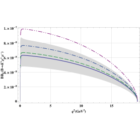
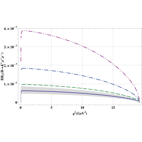
($\mathbf{c}$)	($\mathbf{d}$)

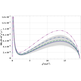
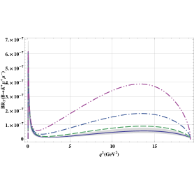
Figure 1: The dependence of the longitudinal and transverse BR for the decay $B\to K^{*}(892)\mu^{+}\mu^{-}$ on $q^{2}$ for different values of $m_{t^{\prime}}$ and $\left|V^{\ast}_{t^{\prime}b}V_{t^{\prime}s}\right|$. In all the graphs, the solid line corresponds to the SM, dashed , dashed dot and dashed double corresponds to $m_{t^{\prime}}=$ 300 GeV, 450 GeV and 600 GeV respectively. $\left|V^{\ast}_{t^{\prime}b}V_{t^{\prime}s}\right|$ has the value 0.005 and 0.015 in $(a)$ and $(b)$ respectively.

($\mathbf{a}$)	($\mathbf{b}$)
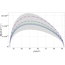
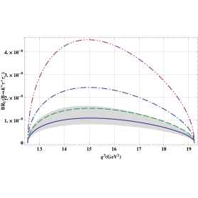
($\mathbf{c}$)	($\mathbf{d}$)

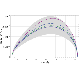
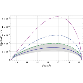
Figure 2: The dependence of the longitudinal and transverse BR for the decay $B\to K^{*}(892)\tau^{+}\tau^{-}$ on $q^{2}$ for different values of $m_{t^{\prime}}$ and $\left|V^{\ast}_{t^{\prime}b}V_{t^{\prime}s}\right|$. Legends and the values of the fourth-generation parameters are the same as in Fig. 1.

($\mathbf{a}$)	($\mathbf{b}$)
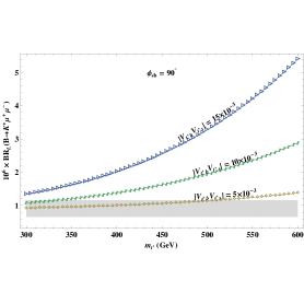
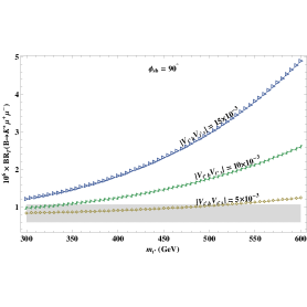
($\mathbf{c}$)	($\mathbf{d}$)

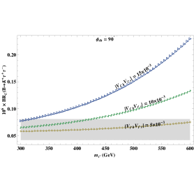
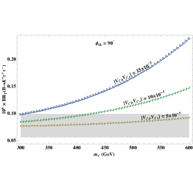
Figure 3: The dependence of the total longitudinal and transverse BR for the decay $B\to K^{*}(892)\mu^{+}\mu^{-}$ on $m_{t^{\prime}}$ for different values of $\left|V^{\ast}_{t^{\prime}b}V_{t^{\prime}s}\right|$.

($\mathbf{a}$)	($\mathbf{b}$)
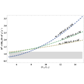
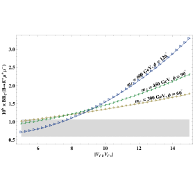
($\mathbf{c}$)	($\mathbf{d}$)

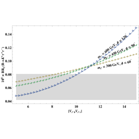
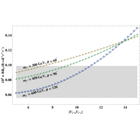
Figure 4: The dependence of the total longitudinal and transverse BR for the decay $B\to K^{*}(892)\mu^{+}\mu^{-}$ on $\left|V^{\ast}_{t^{\prime}b}V_{t^{\prime}s}\right|$ for different values of $m_{t^{\prime}}$.

($\mathbf{a}$)	($\mathbf{b}$)
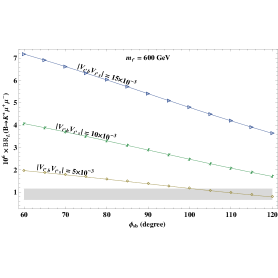
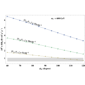
($\mathbf{c}$)	($\mathbf{d}$)

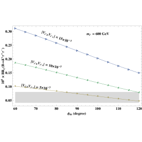
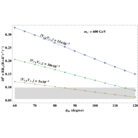
Figure 5: The dependence of the total longitudinal and transverse BR for the decay $B\to K^{*}(892)\mu^{+}\mu^{-}$ on $\phi_{sb}$ for different values of $m_{t^{\prime}}$ and $\left|V^{\ast}_{t^{\prime}b}V_{t^{\prime}s}\right|$.

III.3.2 NP in helicity fractions $f_{L}$ and $f_{T}$

• As for as the study of the polarization of the final state meson $K^{*}$ is concerned in the $B\rightarrow K^{*}l^{+}l^{-}$ decay channel the longitudinal $f_{L}$ and transverse $f_{T}$ helicity fractions become important observable since the uncertainty in this observable is almost negligible, especially when we have muons as the final state leptons. The helicity fraction is the probability of longitudinally and transversely polarized $K^{*}$ meson in the above mentioned decay channel so their sum should be equal to one which can be seen in Figs. 6 and 7. Moreover, in Fig. 6(a,b) we have punched the data points $\bullet$ (black), $\blacksquare$ (red), $\triangledown$ (green) and $\oplus$ (orange) corresponding to the LHCb LHCb , CDF CDF , Belle Belle and Babar babar collaborations, respectively.

• In Fig 6. $f_{L}$ and $f_{T}$ as a function of $q^{2}(GeV^{2})$ for muons as final state leptons are plotted. Here, to check the influence of SM4 on the $f_{L}$ and $f_{T}$ we set $\phi_{sb}=90^{\circ}$ and vary the values of $m_{t^{\prime}}$ and $|V_{t^{\prime}b}V_{t^{\prime}s}|$. Plots 6a and 6b depict that at the minimum value of $m_{t^{\prime}}=300$ GeV the effects in helicity fraction are negligible while at the maximum value of $m_{t^{\prime}}=600$ GeV the effects are mild. Where as the recent results especially from the LHCb and CDF collaboration is favoring the SM predictions as shown in Fig. 6(a,b) and one can also see that the corresponding SM4 curves are very close to some the data points and the deviation to the SM curve is also not robust so the helicity fraction for the case of muons is not a good observable to pin down the status of SM4. Moreover, we have also made the estimate of the average longitudinal helicity fraction of $K^{\ast}$ meson in the low $q^{2}$ bin ($0.1\leq q^{2}\leq 6\text{ GeV}^{2}$) in the SM4 scenario as summarized in the Table 4. One can compare these average values in the low $q^{2}$ bin with that of the experimental value given in Eqs. (26a)-(26d). With the more data available from the LHCb we can use this information to put constraints on the SM4 parameter space.

  Table 4: Average longitudinal helicity fraction $\langle f_{L}\rangle$ of $K^{\ast}$ meson for different values of $m_{t^{\prime}}$ and $|V_{t^{\prime}b}V^{\ast}_{t^{\prime}s}|$, whereas $\langle f_{L}^{SM}\rangle=0.649$.

  $m_{t^{\prime}}$	$|V_{t^{\prime}b}V^{\ast}_{t^{\prime}s}|=5\times 10^{-3}$	$|V_{t^{\prime}b}V^{\ast}_{t^{\prime}s}|=15\times 10^{-3}$
  300	0.653	0.675
  450	0.666	0.715
  600	0.685	0.740

• In contrast to the case of muons the helicity fractions are greatly influenced by SM4 when tauons are the final state leptons as shown in Fig. 7. The effects of SM4 on the $f_{L}$ and $f_{T}$ are clearly distinct from the corresponding SM values in the low $q^{2}$ region, while the NP effects decreased in the high $q^{2}$ region. By a closer look at Figs. 7 (b,d) one can extract that at the maximum values of $m_{t^{\prime}}=600$ GeV and $|V_{t^{\prime}b}V_{t^{\prime}s}|=0.015$ the shift in the minimum(maximum) values of the $f_{T}(f_{L})$ is about 0.2 which lie at $q^{2}=4m^{2}_{\tau}$ and well measured at experiments so this is a good observable to hunt the NP beyond the standard model.

• Now to qualitatively depict the effects of SM4 parameters on $f_{L}$ and $f_{T}$ for the decay $B\rightarrow K^{*}\tau^{+}\tau^{-}$ we have displayed their average values $<f_{L}>$ and $<f_{T}>$ as a function of $m_{t^{\prime}}$, $\phi_{sb}$ and $|V_{t^{\prime}b}V_{t^{\prime}s}|$ in Figs. 8, 9 and 10 respectively. These graphs indicate that the $<f_{L}>$($<f_{T}>$) is the increasing(decreasing) function of SM4 parameters. It is clear from Figs. 8 (a, b) and 10 (a, b) that when we set $\phi_{sb}=90^{\circ},m_{t^{\prime}}=600$ GeV and $|V_{t^{\prime}b}V_{t^{\prime}s}|=0.015$ the value of $<f_{L}>$($<f_{T}>$) is enhanced(reduced) up(down) to $13\%$ approximately. From figs. 9 (a, b) one can extract that at $\phi_{sb}=120^{\circ},m_{t^{\prime}}=600$ GeV and $|V_{t^{\prime}b}V_{t^{\prime}s}|=0.015$ this increment(decrement) in the $<f_{L}>$($<f_{T}>$) values is reached up to $16\%$ to $17\%$ which is quite distinctive and will be observed at LHCb.

($\mathbf{a}$)	($\mathbf{b}$)
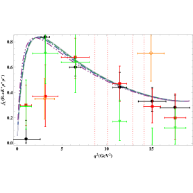
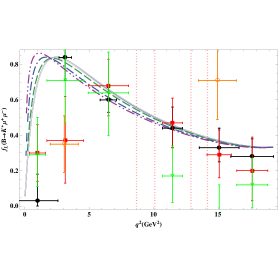
($\mathbf{c}$)	($\mathbf{d}$)

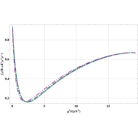
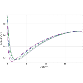
Figure 6: The dependence of the longitudinal and transverse helicity fractions for the decay $B\to K^{*}(892)\mu^{+}\mu^{-}$ on $q^{2}$ for different values of $m_{t^{\prime}}$ and $\left|V^{\ast}_{t^{\prime}b}V_{t^{\prime}s}\right|$. Legends and the values of the fourth-generation parameters are the same as in Fig. 1 while in the graphs in (a) and (b) the data points $\bullet$ (black), $\blacksquare$ (red), $\triangledown$ (green) and $\oplus$ (orange) correspond to the LHCb LHCb , CDF CDF , Belle Belle and Babar babar collaborations, respectively.

($\mathbf{a}$)	($\mathbf{b}$)
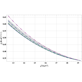
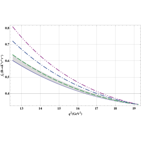
($\mathbf{c}$)	($\mathbf{d}$)

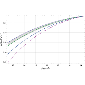
Figure 7: The dependence of the longitudinal and transverse helicity fractions for the decay $B\to K^{*}(892)\tau^{+}\tau^{-}$ on $q^{2}$ for different values of $m_{t^{\prime}}$ and $\left|V^{\ast}_{t^{\prime}b}V_{t^{\prime}s}\right|$. Legends and the values of the fourth-generation parameters are the same as in Fig. 1.

($\mathbf{a}$)	($\mathbf{b}$)

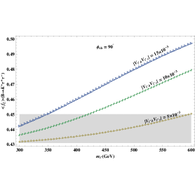
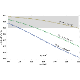
Figure 8: The dependence of the average longitudinal helicity fraction for the decay $B\to K^{*}(892)\tau^{+}\tau^{-}$ on $m_{t^{\prime}}$ and $\phi_{sb}$ for different values of $\left|V^{\ast}_{t^{\prime}b}V_{t^{\prime}s}\right|$.

($\mathbf{a}$)	($\mathbf{b}$)

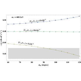
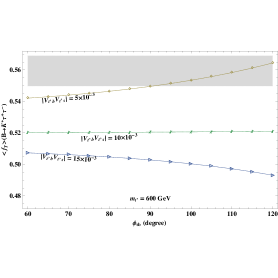
Figure 9: The dependence of the average transverse helicity fraction for the decay $B\to K^{*}(892)\tau^{+}\tau^{-}$ on $m_{t^{\prime}}$ and $\phi_{sb}$ for different values of $\left|V^{\ast}_{t^{\prime}b}V_{t^{\prime}s}\right|$.

($\mathbf{a}$)	($\mathbf{b}$)

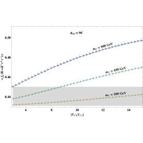
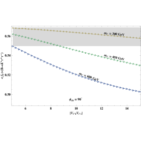
Figure 10: The dependence of the average longitudinal and transverse helicity fractions for the decay $B\to K^{*}(892)\tau^{+}\tau^{-}$ on $\left|V^{\ast}_{t^{\prime}b}V_{t^{\prime}s}\right|$ for different values of $m_{t^{\prime}}$.

IV Summary

The polarization of $K^{*}$ meson in the $B\rightarrow K^{*}\ell^{+}\ell^{-}$ ($\ell=\mu$ or $\tau$) decay is studied from the perspective of SM4. In this respect the polarized branching ratios $BR_{L}$, $BR_{T}$ and the helicity fractions $f_{L},f_{T}$ of $K^{*}$ meson are studied. The explicit dependence of these observables on the $m_{t^{\prime}},|V_{t^{\prime}b}V_{t^{\prime}s}|$ and $\phi_{sb}$ are also discussed. The study showed that the values of these observables are significantly affected by changing the value of SM4 parameters. As we discussed in the numerical analysis, the polarized branching ratios are directly proportional to the SM4 parameters $m_{t^{\prime}}$ and $|V_{t^{\prime}b}V_{t^{\prime}s}|$ and inversely proportional to the CKM4 phase $\phi_{sb}$ . It is found that at the maximum parametric space of SM4 the values of $BR_{L}$ and $BR_{T}$ are enhanced up to 6-7 times of their SM values. Similarly the influence of SM4 parameters on helicity fractions $f_{L}$ and $f_{T}$ and their average values are studied. It is shown that for the case of muons these observables do not show any significant change in their SM values. However, for the case of tauns the effects are quite prominent and well distinct from their SM values. It is also noticed that the effects of SM4 on helicity fractions are decreased when the value of $q^{2}$ is increased and almost vanishes at the maximum value of $q^{2}$. It is also seen that the categorical influence of SM4 parameters $m_{t^{\prime}},|V_{t^{\prime}b}V_{t^{\prime}s}|$ and $\phi_{sb}$ on $\langle f_{L}\rangle$ are constructive and on $\langle f_{T}\rangle$ are destructive. Therefore, the precise measurement of the observables related to the polarization of $K^{*}$ meson, as discussed in this study, not only give us an opportunity to test the SM as well as useful to find out or put some constraint on the SM4 parameters such as $m_{t^{\prime}},|V_{t^{\prime}b}V_{t^{\prime}s}|$ and $\phi_{sb}$. To sum up, the precise study of the polarization of $K^{*}$ meson at LHCb and Tevatron provide us a handy tool to dig out the status of the extra generation of quarks.

References

- (1) Erin De Pree, G. Marshall and Marc Sher, The Fourth Generation t-prime in Extensions of the Standard Model,arXiv: 0906.4500 [hep-ph].
- (2) C. Amsler et al. [Particle Data Group], Phys. Lett. B667 (2008) 1.
- (3) M. Maltoni, V. A. Novikov, L. B. Okun, A. N. Rozanov and M. I. Vysotsky, Phys. Lett. B476 (2000) 107 [arXiv:hep-ph/9911535]; H. J. He, N. Polon- sky and S. f. Su, Phys. Rev. D64 (2001) 053004 [arXiv:hep-ph/0102144]; B. Holdom, Phys. Rev. D54 (1996) 721 [arXiv:hep-ph/9602248].
- (4) G. D. Kribs, T. Plehn, M. Spannowsky and T. M. P. Tait, Phys. Rev. D76 (2007) 075016 [arXiv:0706.3718 [hep-ph]].
- (5) W. S. Hou and C. Y. Ma, Phys. Rev. D82 (2010) 036002.
- (6) S. Bar-Shalom, D. Oaknin and A. Soni, Phys. Rev. D80 (2009) 015011.
- (7) A. J. Buras, B. Duling, T. Feldmann, T. Heidsieck, C. Promberger and S. Recksiegel, JHEP 1009 (2010) 106.
- (8) A. Soni, A. K. Alok, A. Giri, R. Mohanta and S. Nandi, Phys. Lett. B683 (20100 302.
- (9) O. Eberhardt, A. Lenz and J. Rohrwild, Phys. Rev. D82 (2010) 095006.
- (10) A. Soni, A. K. Alok, A. Giri, R. Mohanta and S. Nandi, Phys. Rev. D82 (2010) 033009.
- (11) A. K. Alok, A. Dighe and D. London, Phys. Rev. D83 (2011) 073008.
- (12) B. Holdom, Phys. Rev. Lett. 57 (1986) 2496 [Erratum-ibid. 58 (1987) 177].
- (13) C. T. Hill, M. A. Luty and E. A. Paschos, Phys. Rev. D43 (1991) 3011.
- (14) T. Elliott and S. F. King, Phys. Lett. B283 (1992) 371.
- (15) P. Q. Hung and C. Xiong, Nucl. Phys. B848 (2011) 288.
- (16) B. Holdom, JHEP 0608 (2006) 076.
- (17) P. Q. Hung and M. Sher, Phys. Rev. D77 (2008) 037302.
- (18) P. Q. Hung, C. Xiong, Phys. Lett. B694 (2011) 430.
- (19) P. Q. Hung and C. Xiong, Nucl. Phys. B847 (2011) 160.
- (20) O. Cakir, A. Senol and A. T. Tasci, Europhys. Lett. 88 (2009) 11002.
- (21) B. Holdom, W. S. Hou, T. Hurth, M. L. Mangano, S. Sultansoy and G. Unel, PMC Phys. A3 (2009) 4.
- (22) T. Moroi, Phys. Lett. B493 (2000) 366-374, arXiv:hep-ph/0007328.
- (23) D. Chang, A. Masiero, and H. Murayama, Phys. Rev. D67 (2003) 075013, arXiv:hep-ph/0205111.
- (24) R. Harnik, D. T. Larson, H. Murayama, and A. Pierce, Phys. Rev. D69 (2004) 094024, arXiv:hep-ph/0212180.
- (25) M. Ciuchini, E. Franco, A. Masiero, and L. Silvestrini, Phys. Rev. D67 (2003) 075016, arXiv:hep-ph/0212397.
- (26) J. Foster, K.-i. Okumura, and L. Roszkowski, JHEP 08 (2005) 094, arXiv:hep-ph/0506146.
- (27) M. Blanke, A. J. Buras, B. Duling, S. Gori, and A. Weiler, JHEP 03 (2009) 001, arXiv:0809.1073 [hep-ph].
- (28) M. Blanke, A. J. Buras, B. Duling, K. Gemmler, and S. Gori, JHEP 03 (2009) 108, arXiv:0812.3803 [hep-ph].
- (29) M. Blanke et al., JHEP 12 (2006) 003, arXiv:hep-ph/0605214.
- (30) V. Barger et al., arXiv:0906.3745 [hep-ph].
- (31) C.S. Kim et al., Phys. Lett. B 218 (1989) 343; X. G. He et al., Phys. Rev. D 38 (1988) 814; B. Grinstein et al., Nucl. Phys. B 319 (1989) 271; N. G. Deshpande et al., Phys. Rev. D 39 (1989) 1461; P. J. O’Donnell and H. K. K. Tung, Phys. Rev. D 43 (1991) 2067; N. Paver and Riazuddin, Phys. Rev. D 45 (1992) 978; J. L. Hewett, Phys. Rev. D 53, 4964 (1996); T. M. Aliev, V. Bashiry, and M. Savci, Eur. Phys. J. C 35, 197 (2004); T. M. Aliev, V. Bashiry, and M. Savci, Phys. Rev. D 72, 034031 (2005); T. M. Aliev, V. Bashiry, and M. Savci, J. High Energy Phys. 05 (2004) 037; T. M. Aliev, V. Bashiry, and M. Savci, Phys. Rev. D 73, 034013 (2006); T. M. Aliev, V. Bashiry, and M. Savci, Eur. Phys. J. C 40, 505 (2005); F. Kruger and L. M. Sehgal Phys. Lett. B 380, 199 (1996); Y. G. Kim, P. Ko, and J. S. Lee, Nucl. Phys. B544, 64 (1999); Chuan-Hung Chen and C. Q. Geng, Phys. Lett. B 516, 327 (2001); V. Bashiry, Chin. Phys. Lett. 22, 2201 (2005); W.S. Hou, A. Soni and H. Steger, Phys. Lett. B 192, 441 (1987); W.S. Hou, R.S. Willey and A. Soni, Phys. Rev. Lett. 58, 1608 (1987) [Erratum-ibid. 60, 2337 (1987)]; T. Hattori, T. Hasuike and S. Wakaizumi, Phys. Rev. D 60, 113008 (1999); T.M. Aliev, D.A. Demir and N.K. Pak, Phys. Lett. B 389, 83 (1996); Y. Dincer, Phys. Lett. B 505, 89 (2001) and references therin; C.S. Huang, W.J. Huo and Y.L. Wu, Mod. Phys. Lett. A 14, 2453 (1999); C.S. Huang, W.J. Huo and Y.L. Wu, Phys. Rev. D 64, 016009 (2001); A. K. Alok, et al., JHEP 02 (2010) 053.
- (32) A. Ali, T. Mannel and T. Morosumi, Phys. Lett. B 273, 505 (1991).
- (33) C. W. Chiang, R. H. Li and C. D. Lu, arXiv:0911.2399.
- (34) P. Colangelo, F. De Fazio, R. Feerandes and T. N. Pham, Phys.Rev. D 74 (2006) 115006.
- (35) A. Ahmed, I. Ahmed, M. A. Paracha and A. Rehman, Rev. D 84, 033010 (2011).
- (36) T.M. Aliev, A. Ozpineci, M. Savcı, Phys. Lett. B 511 (2001) 49.
- (37) The LHCb Collaboration, CERN-LHCb-CONF-2011-038, http://cdsweb.cern.ch/record/1367849?ln=en.
- (38) T. Aaltonen et al., [CDF Collaboration], arXiv:1108.0695.
- (39) J. -T. Wei et al., [Belle Collaboration], Phys. Rev. Lett. 103, (2009) 171801.
- (40) B. Aubert et al., [BABAR Collaboration], Phys. Rev. D 79 (2009) 031102 (R).
- (41) A. Ali, P. Ball, L. T. Handoko and G. Hiller, Phys. Rev. D 61, 074024 (2000); [arXiv:hep-ph/9910221].
- (42) G. Buchalla, A. J. Buras and M. E. Lautenbacher, Rev. Mod. Phys. 68 (1996) 1125.
- (43) A. J. Buras and M. Munz, Phys. Rev. D52 (1995) 186; A. J. Buras, M. Misiak, M. Munz and S. Pokorski, Nucl. Phys. B424 (1994) 374.
- (44) A. Ali, T. Mannel and T. Morosumi, Phys. Lett. B 273 (1991) 505.
- (45) C.S. Kim, T. Morozumi, A.I. Sanda, Phys. Lett. B 218 (1989) 343.
- (46) F. Kruger and L. M. Sehgal, Phys. Lett. 380 (1996) 199.
- (47) B. Grinstein, M. J. Savag and M. B. Wise, Nucl. Phys. B319 (1989) 271.
- (48) G. Cella, G. Ricciardi adn A. Vicere, Phys. Lett. B258 (1991) 212.
- (49) C. Bobeth, M. Misiak and J. Urban, Nucl. Phys. B574 (2000) 291.
- (50) H. H. Asatrian, H. M. Asatrian, C. Grueb and M. Walker, Phys. Lett. B507 (2001) 162.
- (51) M. Misiak, Nucl. Phys. B393 (1993) 23, Erratum, ibid. B439 (1995) 461.
- (52) T. Huber, T. Hurth, E. Lunghi, arXiv:0807.1940.
- (53) A. Saddique, M. J. Aslam and C. D. Lu, Eur. Phys. J. C 56 (2008) 267 [arXiv:0803.0192].
- (54) I. Ahmed, M. A. Paracha, M. Junaid, A. Ahmed, A. Rehman and M. J. Aslam, arXiv:1107.5694.
- (55) K. Nakamura et al. (Particle Data Group), J. Phys. G 37 (2010) 075021.
- (56) M. Beneke, T. Feldmann and D. Seidel, Nucl. Phys. B 612 (2001) 25, [hep-ph/0106067].
- (57) A.Soni et al., Phys.Rev. D 82 (2010) 033009 [arXiv:1002.0595]