Current-induced switching in transport through anisotropic magnetic molecules

Abstract

Anisotropic single-molecule magnets may be thought of as molecular switches, with possible applications to molecular spintronics. In this paper, we consider current-induced switching in single-molecule junctions containing an anisotropic magnetic molecule. We assume that the carriers interact with the magnetic molecule through the exchange interaction and focus on the regime of high currents in which the molecular spin dynamics is slow compared to the time which the electrons spend on the molecule. In this limit, the molecular spin obeys a non-equilibrium Langevin equation which takes the form of a generalized Landau-Lifshitz-Gilbert equation and which we derive microscopically by means of a non-equilibrium Born-Oppenheimer approximation. We exploit this Langevin equation to identify the relevant switching mechanisms and to derive the current-induced switching rates. As a byproduct, we also derive S-matrix expressions for the various torques entering into the Landau-Lifshitz-Gilbert equation which generalize previous expressions in the literature to non-equilibrium situations.

I Introduction

In recent years, electronic transport through nanostructures has witnessed a shift toward molecular systems. Several ingenious schemes for measuring transport through single molecules have been realized and experimental control over such systems is rapidly improving. mol A prime difference between transport through single molecules or nanoelectromechanical systems (NEMS) nems as opposed to transport through more conventional nanostructures lies in the coupling of the electronic degrees of freedom responsible for transport to few well-defined collective modes of the molecule, with recent research focusing on effects of molecular vibrations (molecular nanoelectromechanics)nitzan ; molvib ; molvibth and local magnetic moments (molecular spintronics).zuti-2004 ; fert-2008 ; bogani ; fried ; revs

The interesting property of transport setups based on single-molecule magnets is the possibility of combining some classical properties of macroscopic magnets with quantum features such as quantum tunneling. Work on molecular spintronics has focused on single molecule magnets such as Mn₁₂ and transition metal complexes. Transport experiments with Mn₁₂ concentrated on signatures of the magnetic excitations, as revealed by peaks in the differential conductance,jo and a spin-blockade mechanism.mn12 Research on transition metal complexes, based e.g. on Co, also addresses the Kondo effect.kondo Related phenomena have been discussed in molecular spin valves, which have been realized in setups with C₆₀,spin-valv and more recently in TbPc₂ setups coupled to nanotubes through supramolecular interactions . supspin-valv

In addition to their remarkable fundamental quantum transport properties, single molecule magnets are also appealing for their potential as memory cells in spintronics.memcel In this context it is important to have reliable mechanisms for writing and reading the stored information. Specifically, it is essential to have protocols for manipulating and for detecting the orientation of the magnetic moment. To this end it is convenient to take advantage of the coupling between the spin of the electrons, which tunnel from the electrodes, and the localized magnetic moment of the molecule.timm

Much of the existing literature, both on molecular nanoelectromechanics and molecular spintronics, assumes that the electrons reside on the molecule for times large compared to typical vibrational or magnetic precession periods. In this limit, it is often appropriate to treat the dynamics of the system within a rate- or Master equation in the exact eigenstate basis of the isolated molecule,nitzan ; ensslin describing also spin-transfer torques out-of equilibrium.delgado-2010 ; delgado-2010b ; molmagther In the context of nanoelectromechanics, there has recently been much interest in the opposite regime of adiabatic vibrational dynamics, in which the electronic processes are fast compared to the vibrational degrees of freedom, e.g., in the context of certain molecular switches,mozyrsky-2006 ; pistolesi-2008 NEMS near continuous mechanical instabilities,weick-2010 ; weick-2011 flexural modes of suspended carbon nanotubes and graphene,Steele09 or the cooling and amplification of mechanical motion by the backaction of conduction electrons.naik ; stettenheim ; dundas ; lu ; bode-2011 ; bode-2011b

The goal of the present work is to explore the latter limit in the context of magnetic molecules. We consider a generic model for the magnetic molecule, which includes an easy axis anisotropy sandwiched between two metallic (possibly polarized) electrodes at which a bias voltage is applied.fried We focus on the regime where the typical time for dynamics of the molecular magnetic moment is much larger than the dwell time of the electrons flowing through the structure. Within this adiabatic regime it is possible to study the coupled electronic transport and spin dynamics within a non-equilibrium Born-Oppenheimer approximation (NEBO) analogous to the one adopted in NEMS in the equivalent regime.mozyrsky-2006 ; pistolesi-2008 Starting from a microscopic description, we can derive semiclassical equations of motion for the local magnetic moment that have the structure of generalized Landau-Lifshitz-Gilbert (LLG) equations. The latter have been the basis for several previous works in spintronics and nanomagnetism.Katsura06 ; kupferschmidt-2006 ; fransson-2008 ; nunez-2008 ; basko-2009 ; dunn-2011 ; lopez-monis-2012 ; tserkovnyak-2002 ; brataas-2008 ; brataas-2011 ; hals-2010 We note that in previous works describing magnetic nanoparticles, LLG equations have been derived in a perturbative way assuming either that the coupling between the electronic spin and the magnetic moment of the nanoparticle is small Katsura06 ; fransson-2008 ; nunez-2008 and/or that tunneling between the leads and nanoparticle is weak.Katsura06 ; fransson-2008 ; lopez-monis-2012 In contrast, our microscopic derivation relies entirely on the non-equilibrium Born Oppenheimer approximation which is valid in the high-current limit as described above. As a consequence our non-perturbative approach allows us to compute how the parameters of the LLG equation depend on the state of the molecular moment as well as on the applied bias and gate voltages. We mainly focus on two important features. First we analyze the magnetic molecule attached to (non-magnetic) metallic leads. In this case, switching of the molecular moment is induced by the fluctuating torque exerted by the current flow. In addition, we also investigate the renormalization of the switching barrier by the average torque caused by the charge carriers. Second, we consider that switching is dominated by a different mechanism for spin-polarized electrodes, namely by the spin-transfer torque exerted by the transport current. The latter is well known in the context of layered magnetic structures.slonczewski-1996 ; berger-1996 ; spin-torque We also analyze the behavior of the electronic current and we identify in this quantity the interplay between the spin fluctuations and the signatures of coherent transport, which are typical of the molecular devices.

This paper is organized as follows. In Sec. II, we introduce our model of the single-molecule junction containing an anisotropic magnetic molecule. The Landau-Lifshitz-Gilbert equation describing the dynamics of the local moment of the molecule is derived within the NEBO approximation in Sec. III and related to scattering matrix theory in Sec. IV. This Langevin equation is explored in Sec. V. Switching of the molecular moment is discussed in Secs. VI and VII. Section VI focuses on switching caused by fluctuations while Sec. VII discusses situations when the switching is dominated by the spin-transfer torque. We conclude in Sec. VIII. Some technical details are relegated to appendices.

II Model

We consider a minimal model of an anisotropic magnetic molecule embedded into a single-molecule junction.nazarov We assume that transport through the molecule is dominated by a single molecular orbital which is coupled to left ($L$) and right ($R$) leads at different chemical potentials. The spin ${\bf\hat{s}}$ of the current-carrying electrons couples to a localized molecular spin $\hat{\bf M}$ through exchange. Then, the full Hamiltonian

$$H=\sum_{\alpha=L,R}(H_{\alpha}+H_{d\alpha})+H_{d},$$ (1)

encompasses the Hamiltonians

$$H_{\alpha}=\sum_{k_{\alpha},\sigma}\epsilon_{k_{\alpha},\sigma}c^{\dagger}_{k_{\alpha},\sigma}c_{k_{\alpha},\sigma}$$ (2)

of the left ($L$) and right ($R$) leads, modeled as free-electron systems (creation operators $c^{\dagger}_{k_{\alpha},\sigma}$). We will consider the possibility of spin-polarized leads, assuming a spin-dependent dispersion $\epsilon_{k_{\alpha},\sigma}$. The tunneling Hamiltonian

$$H_{d\alpha}=\sum_{k_{\alpha},\sigma}w_{k_{\alpha}}(c^{\dagger}_{k_{\alpha},\sigma}d_{\sigma}+d^{\dagger}_{\sigma}c_{k_{\alpha},\sigma})$$ (3)

describes the hybridization between the molecular orbital (with creation operator $d^{\dagger}_{\sigma}$) and the leads. The molecular Hamiltonian is given by

$$H_{d} = \sum_{\sigma}\epsilon_{0}d^{\dagger}_{\sigma}d_{\sigma}+g_{e}\hat{\bf s}\cdot{\bf B}+J\hat{{\bf s}}\cdot\hat{\bf M}+U(\hat{\bf M}).$$ (4)

The potential experienced by the molecular spin in the absence of coupling to the external leads is $U(\hat{\bf M})=g_{d}\hat{\bf M}\cdot{\bf B}-D{\hat{M}}_{z}^{2}$. The uniaxial anisotropy of the molecule is parametrized through the anisotropy parameter $D$, with easy-axis anisotropy corresponding to $D>0$ and easy-plane anisotropy to $D<0$. The coupling constant $J$ denotes the strength of the exchange interaction between the molecular spin ${\bf\hat{M}}$ and the electronic spins,

$$\hat{s}_{j}=\frac{\hbar}{2}\sum_{\sigma,\sigma^{\prime}}d^{\dagger}_{\sigma}\sigma^{j}_{\sigma\sigma^{\prime}}d_{\sigma^{\prime}},$$ (5)

where $\sigma^{j}$ (with $j=x,y,z$) are the Pauli matrices. For simplicity, we assume this exchange interaction to be isotropic. The energy of the molecular orbital $\epsilon_{0}$ can be tuned by a gate voltage and ${\bf B}$ represents a Zeeman field acting on the electronic and the localized spins with $g$-factors $g_{e}$ and $g_{d}$, respectively.

III Description of the spin dynamics

We now discuss this model in the limit of slow precession of the magnetic moment, that is, many electrons are passing the molecule during a single precessional period of the molecular spin. In this limit, it is natural to approximate the molecular spin as a classical variable whose dynamics can be described within a non-equilibrium Born-Oppenheimer approximation. The resulting dynamics takes the form of a Langevin equation of the Landau-Lifshitz-Gilbert type which we derive microscopically for our model. Specifically, the exchange coupling between the current-carrying electrons and the molecular moment introduces additional torques and damping terms which enter into the Langevin equation and which we will now discuss in detail.

III.1 Semiclassical equation of motion of the molecular spin

Our derivation starts from the Heisenberg equation of motion for the molecular spin,

$$\dot{\hat{M}}_{j} = \sum_{l,k}\varepsilon_{jlk}[J\hat{s}_{l}+g_{d}B_{l}]\hat{M}_{k}$$ (6)

$$+D\sum_{k}\varepsilon_{zjk}[\hat{M}_{z}\hat{M}_{k}+\hat{M}_{k}\hat{M}_{z}],$$

where $\varepsilon_{jlk}$ is the antisymmetric Levy-Civita tensor. Within the non-equilibrium Born-Oppenheimer approximation, we can turn this into an equation of motion for the expectation value ${\bf M}(t)=\langle\hat{\bf M}(t)\rangle$ of the localized spin,

$$\dot{\mathbf{M}}=\mathbf{M}\times\left[-\partial_{\mathbf{M}}U(\mathbf{M})-J\mathbf{s}+\boldsymbol{\delta{\cal B}}\right],$$ (7)

with $-\partial_{\mathbf{M}}U(\mathbf{M})=-g_{d}\mathbf{B}+2DM_{z}\hat{\mathbf{e}}_{z}$. Here, ${\bf M}={\bf M}(t)$ denotes the molecular spin averaged over a time interval large compared to the electronic time scales, but small compared to the precessional dynamics of the molecular spin itself. The corresponding time-averaged electronic spin ${\bf s}={\bf s}(t)$ can be expressed in terms of the electronic lesser Green’s function

$${G}_{\sigma\sigma^{\prime}}^{<}(t,t^{\prime})=i\langle d^{\dagger}_{\sigma^{\prime}}(t^{\prime})d_{\sigma}(t)\rangle$$ (8)

of the molecular orbital as

$$s_{j}(t)=\langle\hat{s}_{j}\rangle_{{\bf M}(t)}=-\frac{i\hbar}{2}\mbox{tr}[G^{<}(t,t){\sigma}^{j}].$$ (9)

It is important to note that due to the Born-Oppenheimer approximation, the lesser Green’s function must be evaluated for a given time dependence of the molecular spin ${\bf M}(t)$. As a result, the average electronic spin ${\bf s}(t)$ depends on the molecular spin at earlier times. This will be considered in more detail in the next subsection. The instantaneous contribution gives rise to a force acting on the molecular spin. Retardation effects produce terms proportional to $\dot{\mathbf{M}}$, appearing in the equation of motion as Gilbert damping and a change in the gyromagnetic ratio. Additionally, fluctuations of the electron spin give rise to a fluctuating Zeeman field $\boldsymbol{\delta{\cal B}}$ acting on the molecular spin.

III.2 Electronic Green’s function in the adiabatic limit

We now turn to evaluate the electronic lesser Green’s function, accounting for the slowly varying molecular spin ${\bf M}(t)$. We start by considering the corresponding retarded Green’s function

$${G}^{R}_{\sigma,\sigma^{\prime}}(t,t^{\prime})=-i\theta(t-t^{\prime})\langle\{d_{\sigma}(t),d^{\dagger}_{\sigma^{\prime}}(t^{\prime})\}\rangle.$$ (10)

Since the electrons are non-interacting, we can obtain ${G}^{<}$ from ${G}^{R}$ at the end of the calculation. From now on, we set $\hbar=1$. The retarded Green’s function satisfies the Dyson equationjauho

$$(-i\partial_{t^{\prime}}-\epsilon_{0}){G}^{R}_{\sigma\sigma^{\prime}}(t,t^{\prime})-\int dt_{1}\sum_{\sigma_{1}}{G}^{R}_{\sigma\sigma_{1}}(t,t_{1})\Sigma^{R}_{\sigma_{1}\sigma^{\prime}}(t_{1},t^{\prime})\\ -\sum_{\sigma_{1}}G^{R}_{\sigma\sigma_{1}}(t,t^{\prime}){\boldsymbol{\sigma}}_{\sigma_{1}\sigma^{\prime}}\cdot{\bf b}(t^{\prime})=\delta(t-t^{\prime})\delta_{\sigma\sigma^{\prime}}.$$ (11)

Here we introduce the self-energy

$$\Sigma^{R}_{\sigma,\sigma^{\prime}}(t,t^{\prime})=\delta_{\sigma\sigma^{\prime}}\sum_{\alpha}\int\frac{d\omega}{2\pi}\Sigma^{R}_{\alpha,\sigma}(\omega)e^{-i\omega(t-t^{\prime})}$$ (12)

with

$$\Sigma^{R}_{\alpha,\sigma}(\omega)=\sum_{k_{\alpha}}|w_{k_{\alpha}}|^{2}\frac{1}{\omega-\epsilon_{k_{\alpha},\sigma}+i\eta}$$ (13)

accounting for the coupling to the (possibly spin-polarized) leads, see also Appendix A. It is convenient to introduce an effective magnetic field experienced by the electrons given by

$$\mathbf{b}(t)=\frac{1}{2}(J{\bf M}(t)+g_{e}{\bf B}).$$ (14)

Notice that even if we consider a constant external magnetic field, the effective magnetic field is time dependent due to the explicit time dependence of the molecular spin $\mathbf{M}=\mathbf{M}(t)$.

In order to implement the Born-Oppenheimer approximation, it is convenient to rewrite the Dyson equation in the mixed (Wigner) representation defined by

$$\tilde{O}(t,\omega)\equiv\int\mathrm{d}\tau\,\mathrm{e^{i\omega\tau}O(t+\tau/2,t-\tau/2)},$$ (15)

for a general quantity $O(t_{1},t_{2})$ depending on two times with central and relative times defined as $t=(t_{1}+t_{2})/2$ and $\tau=t_{1}-t_{2}$. The non-equilibrium Born-Oppenheimer approximation can now be implemented by noting that the dependence on the central time $t$ is slow. Thus, convolutions such as $C(t_{1},t_{2})=\int\mathrm{d}t_{3}\,C_{1}(t_{1},t_{3})C_{2}(t_{3,}t_{2})$ can be approximated in Wigner representation through

$$\tilde{C}(t,\omega) =\exp\left[\frac{i}{2}\left(\partial_{\omega}^{\tilde{C_{1}}}\partial_{t}^{\tilde{C_{2}}}-\partial_{t}^{\tilde{C}_{1}}\partial_{\omega}^{\tilde{C}_{2}}\right)\right]\tilde{C}_{1}\tilde{C}_{2}$$

$$\simeq\tilde{C}_{1}\tilde{C}_{2}+\frac{i}{2}\left(\partial_{\omega}\tilde{C}_{1}\partial_{t}\tilde{C}_{2}-\partial_{t}\tilde{C}_{1}\partial_{\omega}\tilde{C}_{2}\right)$$ (16)

in next-to-leading order using the shorthand $\tilde{C}_{l}=\tilde{C}_{l}(t,\omega)$.

For our problem, to lowest order in the slow changes of $\bf{M}$, we then obtain for the Dyson equation

$$1 = G^{R}\left(\omega-\epsilon_{0}-\Sigma^{R}-\boldsymbol{\sigma}\cdot\mathbf{b}\right)$$ (17)

$$-\frac{i}{2}\partial_{\omega}G^{R}\partial_{t}\boldsymbol{\sigma}\cdot\mathbf{b}-\frac{i}{2}\partial_{t}G^{R}\left(1-\partial_{\omega}\Sigma^{R}\right)$$

where $G^{R}=G^{R}(t,\omega)$ denotes the Green’s function in the Wigner representation. In the above equation and in what follows, the Green’s functions, as well as the self-energy, are matrices in spin space with elements $G^{R}_{\sigma,\sigma^{\prime}}(t,\omega)$ and $\Sigma^{R}_{\sigma,\sigma^{\prime}}(\omega)$, respectively. In the strictly adiabatic limit we drop the terms proportional to derivatives with respect to the central time. To this order we obtain

$$G_{0}^{R}(\mathbf{M},\omega)=\left[\omega-\epsilon_{0}-\Sigma^{R}(\omega)-\boldsymbol{\sigma}\cdot\mathbf{b}\right]^{-1}.$$ (18)

In next-to-leading order in the Born-Oppenheimer approximation, we keep the time derivatives with respect to central time to linear order. Equation (18) implies $[\partial_{t}G_{0}^{R}]^{-1}=-\boldsymbol{\sigma}\cdot\dot{\mathbf{b}}$. Accordingly, by differentiating $\left[\omega-\epsilon_{0}-\Sigma^{R}(\omega)-\boldsymbol{\sigma}\cdot\mathbf{b}\right]G_{0}^{R}=1$ with respect to time and multiplying the resulting equation with $G_{0}^{R}$ one obtains the identity $\partial_{t}G_{0}^{R}=G_{0}^{R}\boldsymbol{\sigma}\cdot\dot{\mathbf{b}}G_{0}^{R}$. Then the Dyson equation yields

$$G^{R}\simeq G_{0}^{R}+\frac{i}{2}\left[\partial_{\omega}G^{R}_{0}\boldsymbol{\sigma}\cdot\dot{\mathbf{b}}G^{R}_{0}-G^{R}_{0}\boldsymbol{\sigma}\cdot\dot{\mathbf{b}}\partial_{\omega}G^{R}_{0}\right].$$ (19)

The lesser Green’s function can now be deduced from the relation $G^{<}=G^{R}\otimes\Sigma^{<}\otimes G^{A}$,jauho where $\otimes$ denotes integration over internal time arguments and $G^{A}=[G^{R}]^{\dagger}$. The lesser self-energy depends only on time differences,

$$\Sigma_{\sigma,\sigma^{\prime}}^{<}(\omega)=i\delta_{\sigma,\sigma^{\prime}}\sum_{\alpha}f_{\alpha}(\omega)\Gamma_{\alpha,\sigma}(\omega).$$ (20)

Here, we introduced $\Gamma_{\alpha,\sigma}(\omega)=-2\mbox{Im}[\Sigma^{R}_{\alpha,\sigma}(\omega)]$ as well as the Fermi functions $f_{\alpha}(\omega)=1/(1+e^{\beta_{\alpha}(\omega-\mu_{\alpha})})$ with $\alpha=L,R$. We obtain after straightforward algebra

$$G^{<}\simeq G_{0}^{<}+\frac{i}{2}\Bigl{(}\partial_{\omega}G_{0}^{<}\boldsymbol{\sigma}\cdot\dot{\mathbf{b}}G_{0}^{A}-G_{0}^{<}\boldsymbol{\sigma}\cdot\dot{\mathbf{b}}\partial_{\omega}G_{0}^{A}\\ +\partial_{\omega}G_{0}^{R}\boldsymbol{\sigma}\cdot\dot{\mathbf{b}}G_{0}^{<}-G_{0}^{R}\boldsymbol{\sigma}\cdot\dot{\mathbf{b}}\partial_{\omega}G_{0}^{<}\Bigr{)}.$$ (21)

Here we used $G_{0}^{<}=G_{0}^{R}\Sigma^{<}G_{0}^{A}$ and suppressed the arguments of the frozen Green’s functions, $G_{0}^{R,A,<}=G_{0}^{R,A,<}(\bf{M},\omega)$.

III.3 Electron spin

We can now employ this result for the electronic Green’s function and evaluate the electron spin. Substituting Eq. (21) into Eq. (9), we find

$$J\mathbf{s}({\bf M}) \simeq J\mathbf{s}^{0}({\bf M})+\gamma({\bf M})\dot{\mathbf{M}}.$$ (22)

The first term in (22) contains the average electron spin

$$s^{0}_{l}({\bf M})=-\frac{i}{2}\int\frac{d\omega}{2\pi}\mbox{tr}[G_{0}^{<}\sigma^{l}]$$ (23)

in the strictly adiabatic limit. The correction due to retardation effects associated with the slow dynamics of the molecular spin are captured by the matrix $\gamma({\bf M})$,

$$\gamma^{lk}({\bf M})= \frac{J^{2}}{4}\int\frac{d\omega}{2\pi}\Bigl{\{}\mbox{tr}[\partial_{\omega}G_{0}^{>}\sigma^{k}G_{0}^{<}\sigma^{l}]$$

$$\quad+\mbox{tr}[\partial_{\omega}G_{0}^{A}\left(\sigma^{k}G_{0}^{<}\sigma^{l}-\sigma^{l}G_{0}^{<}\sigma^{k}\right)]\Bigr{\}},$$ (24)

where we have integrated by parts and used the greater Green’s function

$$G^{>}_{\sigma\sigma^{\prime}}(t,t^{\prime})=-i\langle d_{\sigma}(t)d_{\sigma^{\prime}}^{\dagger}(t^{\prime})\rangle,$$ (25)

with the relation $G^{>}-G^{<}=G^{R}-G^{A}$. It is appropriate to split this matrix into $\gamma^{lk}=\gamma^{lk}_{s}+\gamma^{lk}_{a}$ with the shorthand $\gamma^{lk}_{s,a}=(\gamma^{lk}\pm\gamma^{kl})/2$, see Eqs. (69) and (70). As we will see, the symmetric part $\gamma^{lk}_{s}$ describes Gilbert damping of the molecular spin, induced by the coupling to the electrons while the antisymmetric part $\gamma^{lk}_{a}$ will induce a coupling renormalization.

Due to the stochastic nature of the current flow through the magnetic molecule (as reflected in thermal as well as shot noise of the current), the electronic spin will also fluctuate, giving rise to a fluctuating torque $\boldsymbol{\delta{\cal B}}(t)$ acting on the molecular spin. Using Wick’s theorem we obtain for the symmetrized correlator

$$\langle\delta B_{k}(t)\delta B_{m}(t^{\prime})\rangle=\frac{J^{2}}{4}\mbox{tr}[\sigma^{k}G^{>}(t,t^{\prime})\sigma^{m}G^{<}(t^{\prime},t)]_{s}$$ (26)

of the electron spin. In the Born-Oppenheimer approximation, the fluctuations of the spin, as given by Eq. (26), can be evaluated using the Green’s function $G^{<,>}_{0}$ to lowest order in $\dot{\mathbf{b}}$. Thus, the fluctuating Zeeman field $\boldsymbol{\delta{\cal B}}$ has the symmetrized correlator $\langle\delta{\cal B}_{k}(t)\delta{\cal B}_{l}(t^{\prime})\rangle=\tilde{D}^{kl}(\mathbf{M})\delta(t-t^{\prime})$ with

$$\tilde{D}^{kl}(\mathbf{M})=\frac{J^{2}}{4}\int\frac{d\omega}{2\pi}\mbox{tr}[\sigma^{k}G_{0}^{>}\sigma^{l}G_{0}^{<}]_{s}.$$ (27)

Note that in the Born-Oppenheimer limit, we can neglect any frequency dependence of this correlation function on the time scales of the molecular spin, so that the fluctuating Zeeman field can be taken as locally correlated in time.

III.4 Landau-Lifshitz-Gilbert equation

Substituting the expression for the electronic spin (22) into the equation of motion (7) we obtain a Langevin equation of the Landau-Lifshitz-Gilbert type,

$$\dot{\bf M}={\bf M}\times\left[-\partial_{\mathbf{M}}U-J\mathbf{s}^{0}-\gamma_{s}\dot{\bf M}-\gamma_{a}\dot{\bf M}+\boldsymbol{\delta{\cal B}}\right].$$ (28)

Note that, unlike in simple versions of a Landau-Lifshitz-Gilbert equation, the effective exchange field ${\bf s}^{0}$ as well as the coefficient matrices $\gamma_{s}$ and $\gamma_{a}$ still depend on the molecular spin ${\bf M}$ itself. We can simplify this equation by introducing the vector

$$C_{k}(\mathbf{M}) =\frac{1}{2}\sum_{lm}\epsilon_{klm}\gamma^{lm}_{a}(\mathbf{M}).$$ (29)

Using that the length of $\mathbf{M}$ is conserved, it follows that the antisymmetric part of $\gamma$ merely renormalizes the precession frequency by an overall prefactor

$$\alpha(\mathbf{M}) =\frac{1}{1+\mathbf{C}\cdot\mathbf{M}}.$$ (30)

This yields the simplified Landau-Lifshitz-Gilbert equation

$$\dot{\bf M}=\alpha{\bf M}\times\left[-\partial_{\mathbf{M}}U-J\mathbf{s}^{0}-\gamma_{s}\dot{\bf M}+\boldsymbol{\delta{\cal B}}\right],$$ (31)

which we will analyze further in the subsequent sections.

When coupled to spin-polarized leads and when a finite bias voltage is applied, the torque can be non-conservative, yielding the so-called spin-transfer torque.spin-torque Also the eigenvalues of $\gamma_{s}$ can become overall negative, providing another mechanism of energy transfer from the electrons to the localized spin.

It is interesting to compare these results with those for the related problem of charge carriers interacting with a slow vibrational degree of freedom in a NEMS. In both cases, the dynamics of the slow collective degree of freedom can be described in terms of a Langevin equation.mozyrsky-2006 ; pistolesi-2008 Since the stochastic spin dynamics is effectively two-dimensional, it generically exhibits similar phenomena as NEMS with more than one vibrational mode.dundas ; lu ; bode-2011 Specifically, this includes the non-conservative nature of the average force in general non-equilibrium situations as well as the presence of the antisymmetric contribution to the velocity-dependent force. The latter Berry phase contributionberry acts, however, in different ways in the two cases, owing to the different orders of the Langevin equation. In the vibrational context, this term gives rise to an effective Lorentz force, while it merely renormalizes the precession frequency in the context of the magnetic molecule.

IV Relation to scattering matrix theory

Before proceeding with analyzing the Landau-Lifshitz-Gilbert equation (31) in more detail, we pause to provide S-matrix expressions for the various entries into this equation. It has already been noted in a series of works by Brataas et al.tserkovnyak-2002 ; brataas-2008 ; brataas-2011 ; hals-2010 that the coefficients in the Landau-Lifshitz-Gilbert equation in lead-ferromagnet-lead structures can be expressed in terms of the scattering matrix of the structure, resulting in expressions for Gilbert damping and the fluctuating torque in thermal equilibrium and for current-induced spin-transfer torques within linear response theory. Here we will provide S-matrix expressions which remain valid in general out-of-equilibrium situations and which include the exchange field and the precession renormalization in addition to the Gilbert damping with the only assumption that the precessional frequency of the localized magnetic moment is slow compared to the electronic time scales. Our discussion here closely follows recent work on current-induced forces in nanoelectromechanical systems.bode-2011 ; bode-2011b

For adiabatic parameter variations, the full ${\cal S}$-matrix of mesoscopic conductors can be expressed in the Wigner representation as ${\cal S}(t,\omega)=1-2\pi i(W{G}^{R}W^{\dagger})(t,\omega)$. Expanding ${\cal S}$ to linear order in the velocities $\dot{\bf M}$ of the adiabatic variables, Moskalets and Büttiker moskalets-2004 ; arrachea-2006 introduced an $A$-matrix through

$${\cal S}(t,\omega)\simeq S({\bf M}(t),\omega)+\dot{\mathbf{M}}(t)\cdot\mathbf{A}({\bf M}(t),\omega).$$ (32)

For the model considered here, the frozen $S$-matrix is readily related to the frozen retarded Green’s function $G_{0}^{R}({\bf M},\omega)$ through nazarov

$$S({\bf M},\omega)=1-2\pi iWG_{0}^{R}({\bf M},\omega)W^{\dagger}$$ (33)

while the $A$-matrix is given by

$$A_{k}({\bf M},\omega)=\pi\frac{J}{2}\Bigl{[} \partial_{\omega}\left(WG_{0}^{R}\right)\sigma^{k}G_{0}^{R}W^{\dagger}$$

$$\qquad-WG_{0}^{R}\sigma^{k}\partial_{\omega}\left(G_{0}^{R}W^{\dagger}\right)\Bigr{]}.$$ (34)

The average electronic spin $s^{0}_{l}({\bf M})$ can be written in terms of the frozen $S$-matrix (33) by expressing the lesser Green’s function $G_{0}^{<}=G_{0}^{R}\Sigma^{<}G_{0}^{A}$ in terms of the self-energy $\Sigma^{<}(\omega)=i\pi\sum_{\alpha}f_{\alpha}W^{\dagger}\Pi_{\alpha}W$ with $\Pi_{\alpha}$ a projector on lead $\alpha$. Using the identity $2\pi iW^{\dagger}W=(G^{R})^{-1}-(G^{A})^{-1}$, we then find

$$Js^{0}_{k}({\bf M})=-\sum_{\alpha}\int\frac{d\omega}{2\pi i}f_{\alpha}\ {\rm Tr}\left(\Pi_{\alpha}S^{\dagger}\frac{\partial S}{\partial M_{k}}\right)$$ (35)

for the average electronic spin. Here the trace “Tr” acts in lead-channel space.

The S-matrix expression (35) allows us to make some general statements about the average torque acting on the molecular spin. In particular, we can evaluate the curl of the average torque,

$$\frac{\partial(Js^{0}_{k})}{\partial M_{l}}-\frac{\partial(Js^{0}_{l})}{\partial M_{k}}=i\sum_{\alpha}\int\frac{d\epsilon}{\pi}f_{\alpha}{\rm Tr}\left(\Pi_{\alpha}\frac{\partial S^{\dagger}}{\partial M_{l}}\frac{\partial S}{\partial M_{k}}\right)_{a}.$$ (36)

In thermal equilibrium, Eq. (36) can be turned into a trace over a commutator of finite-dimensional matrices due to the relations $f_{\alpha}=f$, $\sum_{\alpha}\Pi_{\alpha}=1$, and unitarity $S^{\dagger}S={\bf 1}$. This implies that $\partial(S^{\dagger}S)/\partial M_{k}=0$ so that there is no spin-transfer torque. In general out-of-equilibrium situations, the curl will be nonzero, giving rise to finite spin-transfer torque.

Similar to the average spin, we can also express the variance of the fluctuating Zeeman field (27) in terms of the frozen $S$-matrix,

$$\tilde{D}^{kl}({\bf M})= \sum_{\alpha\alpha^{\prime}}\int\frac{d\omega}{2\pi}f_{\alpha}(1-f_{\alpha^{\prime}})$$

$$\times{\rm Tr}\left\{\Pi_{\alpha}\left(S^{\dagger}\frac{\partial S}{\partial M_{k}}\right)^{\dagger}\Pi_{\alpha^{\prime}}S^{\dagger}\frac{\partial S}{\partial M_{l}}\right\}_{s}.$$ (37)

By going to a basis in which $\tilde{D}$ is diagonal and using $\Pi_{\alpha}=\Pi_{\alpha}^{2}$, we find that $\tilde{D}$ is a positive definite matrix.

To express the velocity-dependent forces in terms of the scattering matrix in general non-equilibrium situations, we need to go beyond the frozen scattering matrix $S$ and include the $A$ matrix introduced above. The Gilbert-damping coefficients appearing in the Langevin equation (31) can then be written as

$$\gamma_{s}^{kl}({\bf M})=\sum_{\alpha}\int\frac{d\omega}{4\pi}(-\partial_{\omega}f_{\alpha}){\rm Tr}\left\{\Pi_{\alpha}\frac{\partial S^{\dagger}}{\partial M_{k}}\frac{\partial S}{\partial M_{l}}\right\}_{s}$$

$$+\sum_{\alpha}\int\frac{d\omega}{2\pi i}f_{\alpha}{\rm Tr}\left\{\Pi_{\alpha}\left(\frac{\partial S^{\dagger}}{\partial M_{k}}A_{l}-A^{\dagger}_{l}\frac{\partial S}{\partial M_{k}}\right)\right\}_{s}.$$ (38)

The eigenvalues of the first line are strictly positive while the sign of the second line is not fixed, giving rise to the possibility of overall negative Gilbert damping. Note that the second line is a pure non-equilibrium contribution. This can be seen by using unitarity of $S$ as well as ${\cal S}$, implying moskalets-2004 ; arrachea-2006 ${\bf A}S^{\dagger}+S{\bf A}^{\dagger}=(i/2)[\partial_{\bf M}S\partial_{\omega}S^{\dagger}-\partial_{\omega}S\partial_{\bf M}S^{\dagger}]$. With this preparation, it is now easy to ascertain that in equilibrium damping and fluctuations are related by the fluctuation-dissipation theorem, $\tilde{D}^{kl}=2T\gamma^{kl}_{s}$.

Similarly, we express the antisymmetric part of $\gamma^{kl}$ as

$$\gamma_{a}^{kl}({\bf M})=\sum_{\alpha}\int\frac{d\omega}{2\pi i}f_{\alpha}{\rm Tr}\left\{\Pi_{\alpha}\left(S^{\dagger}\frac{\partial A_{k}}{\partial M_{l}}-\frac{\partial A^{\dagger}_{k}}{\partial M_{l}}S\right)\right\}_{a},$$ (39)

which causes a renormalization of the precession frequency, as discussed above.

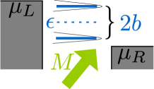
Figure 1: (Color online) Illustration of the setup. The electronic level splits due to the effective magnetic field, given by $b=b(\vartheta)$. The number of levels in the current window depends on $b$, the applied bias voltage $eV=\mu_{L}-\mu_{R}$ and the gate voltage $eV_{\mathrm{g}}=(\mu_{L}+\mu_{R})/2-\epsilon$. It changes from zero ($eV/2>eV_{\mathrm{g}}\pm b$) to one ($eV_{\mathrm{g}}+b>eV/2>eV_{\mathrm{g}}-b$) to two ($eV_{\mathrm{g}}\pm b>eV/2$) [assuming $eV,eV_{\mathrm{g}}>0$].

V Molecular switches with axial symmetry

From now on we specify to the case of axial symmetry, where both the magnetic field and the polarization of the leads point along the anisotropy axis. In this section, we will derive explicit expressions for the current-induced forces, including their dependence on the molecular spin $\mathbf{M}$.

We first consider the average torque which is determined by the average electronic spin. Given that there are two basic vectors in the problem, namely $\hat{\bf e}_{z}$ and $\hat{\mathbf{M}}=\mathbf{M}/M$, the spin can be decomposed as

$${\bf s}^{0}({\bf M})=s_{M}({\bf M})\hat{{\bf M}}+s_{z}({\bf M})\hat{\bf e}_{z}+s_{t}({\bf M})(\hat{\bf e}_{z}\times\hat{{\bf M}}).$$ (40)

Hence, the average torque exerted on the molecular spin by the conduction electrons is

$$-\alpha{\bf M}\times J\mathbf{s}^{0}=-\alpha{\bf M}\times\left[s_{z}\,\hat{\bf e}_{z}+s_{t}\,(\hat{\bf e}_{z}\times\hat{{\bf M}})\right]$$ (41)

which is obtained by inserting Eq. (40) into the Landau-Lifshitz-Gilbert equation (31). The first term inside the bracket can be derived from a potential, since its curl vanishes. This becomes more evident from the explicit expressions below using that the $\mathbf{M}$-dependence of the coefficients stems from the effective magnetic field $\mathbf{b}$ experienced by the electrons and that the length of $\mathbf{M}$ is conserved. This contribution modifies the precession frequency around the $z$-axis. In contrast, the second term on the right hand side of Eq. (41) has a non-vanishing curl, $\nabla_{\mathbf{M}}\times\left[s_{t}\,(\hat{\bf e}_{z}\times\hat{{\bf M}})\right]\neq 0$, so that $s_{t}$ introduces a non-conservative torque, providing the possibility of energy exchange between the conduction electrons and the molecule.

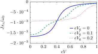
Figure 2: (Color online) Component of the average current-induced torque in a uniaxial situation for unpolarized leads. $Js_{z}(\mathbf{M})$ is plotted as a function of the applied bias voltage for different gate voltages $eV_{\mathrm{g}}$. As discussed in the text, $Js_{z}$ changes when the number of levels in the current window varies at $V_{\mathrm{g}}\pm eV/2=\pm b$ (see also Fig. 1). The plots are obtained at zero temperature at the potential minimum $\vartheta=0$ for the values $JM/2=0.2$, $\Gamma=0.1$, $g_{e}B/2=0.002$ and $g_{e}=g_{d}$. The precession frequency in the absence of coupling to electron spin and magnetic field is $\omega_{0}=2DM=0.01$. All energies are measured in units of the barrier height without magnetic field $DM^{2}$.

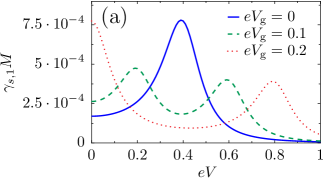
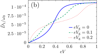
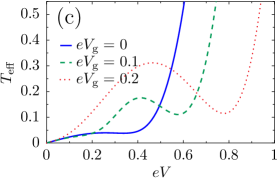
Figure 3: (Color online) Damping and fluctuations as a function of the applied bias voltage. (a) The damping coefficient $\gamma_{s,1}$ is plotted for three different gate voltages. It is peaked when the number of levels in the current region changes from zero to one to two at $V_{\mathrm{g}}\pm eV/2=\pm b$ (see also Fig. 1). (b) At these points the fluctuation kernel $\tilde{D}_{1}$ increase steplike. The level broadening results from the interaction with the leads encapsulated in $\Gamma$. (c) The effective temperature $T_{\mathrm{eff}}=\tilde{D}_{1}/(2\gamma_{s,1})$ is shown as a function of the bias voltage. The plots are obtained at the potential minimum $\vartheta=0$ with the same parameters as in Fig. 2. All energies are measured in units of the barrier height without magnetic field $DM^{2}$.

Concrete expressions for these contributions to the current-induced torque can be obtained from

$$s_{z}({\bf M})= -i\int\frac{d\omega}{2\pi}[G^{<}_{z}({\bf M},\omega)$$

$$+G^{<}_{b}({\bf M},\omega)\Bigl{(}\frac{g_{e}B}{2}+\mbox{Re}[\Sigma_{s}^{R}]\Bigr{)}],$$ (42)

$$s_{t}({\bf M})= -\frac{iJ}{M}\int\frac{d\omega}{2\pi}G^{<}_{t}({\bf M},\omega),$$ (43)

as derived by substituting Eq. (65) into Eq. (23) and taking into account possibly spin-polarized leads with the notation $\Sigma^{R}_{\alpha,c(s)}=[\Sigma^{R}_{\alpha,\uparrow}\pm\Sigma^{R}_{\alpha,\downarrow}]/2$ for the self-energies.

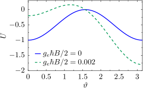
Figure 4: (Color online) Potential experienced by the molecular spin in the absence of coupling to the electrons. $U(\vartheta)$ is shown for different magnetic fields. All energies are measured in units of the barrier height without magnetic field $DM^{2}$.

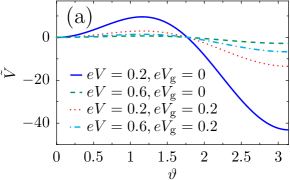
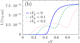
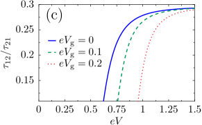
Figure 5: (Color online) Switching dynamics for unpolarized leads. (a) $\tilde{V}$ is plotted for different bias and gate voltages. (b) The switching rate $1/\tau_{12}$ is plotted as a function of the applied bias voltage for different gate voltages. (c) The ratio between the switching rates $1/\tau_{21}$ and $1/\tau_{12}$ is shown. The plots are obtained with the same parameters as in Fig. 2. All energies are measured in units of the barrier height without magnetic field $DM^{2}$.

These general expressions simplify significantly for unpolarized leads, which corresponds to $\Sigma^{R}_{\alpha,s}=0$. Indeed, one finds that then $G^{<}_{t}$ and $G^{<}_{z}$ vanish, see Eq. (A). This implies in particular that the component $s_{t}$ of the average torque vanishes. The remaining conservative contribution $s_{z}$ is then found to be $s_{z}=s_{z}^{-}-s_{z}^{+}$ with

$$s_{z}^{\pm}(\mathbf{M})= \sum_{\alpha}\frac{\Gamma_{\alpha}}{\pi\Gamma}\Bigl{(}\arctan\left[\frac{\mu_{\alpha}-\epsilon\pm b}{\Gamma/2}\right]+\frac{\pi}{2}\Bigr{)}\frac{g_{e}B}{2b}.$$ (44)

Here we assume the limit of zero temperature and introduce the shorthand $\epsilon=\epsilon_{0}+\mbox{Re}[\Sigma_{c}]$.

It is instructive to study the dependence of the average torque on bias and gate voltage. Notice that, due to the effective magnetic field acting on the electron spin, the electronic level splits, see Fig. 1. The average torque is finite when just one level, corresponding to e.g. spin-up electrons, is occupied. In contrast, for sufficiently high bias voltages both spin-up and spin-down electrons participate in the transport so that no net electron spin acts on the molecule. This is illustrated in Fig. 2, where the average electronic spin on the molecule is plotted as a function of the applied bias voltage $eV$ for three different values of the molecular level $\epsilon_{0}$ (as tunable by the gate voltage $eV_{\mathrm{g}}$).

For Gilbert damping and the fluctuating torque, we restrict ourselves to unpolarized leads. This choice is motivated by the fact that switching of the molecular spin (as discussed in the next two sections) is dominated by the average torque for polarized leads (and thus weakly affected by higher orders in the adiabatic expansion) and by the fluctuating force for unpolarized leads. (We mention in passing that expressions for Gilbert damping and fluctuating force for polarized leads can be readily derived but are rather cumbersome.)

For unpolarized leads, we can split the Gilbert damping tensor into one part proportional to the unit matrix and another proportional to a projector onto the $z$-axis,

$${\bf M}\times\gamma_{s}\dot{{\bf M}}=\gamma_{s,1}{\bf M}\times\dot{\mathbf{M}}+\gamma_{s,2}(\dot{\mathbf{M}}\cdot\hat{\mathbf{e}}_{z}){\bf M}\times\hat{\mathbf{e}}_{z},$$ (45)

where $\gamma_{s,1}$ and $\gamma_{s,2}$ are scalars. The first term in Eq. (45) tends to (anti-)align the molecular spin with the anisotropy axis while the second modifies the precession frequency.

The coefficients $\gamma_{s,1}$ and $\gamma_{s,2}$ are calculated by inserting $G_{0}^{<}$ and $G_{0}^{>}$ from Eq. (A) into Eq. (A), resulting in

$$\gamma_{s,1}(\mathbf{M})=\int\frac{d\omega}{8\pi}\sum_{\alpha\beta}\frac{J^{2}\,\Gamma_{\alpha}\Gamma_{\beta}(-\partial_{\omega}f_{\beta})}{\prod_{\pm}\left[(\omega-\epsilon\pm b)^{2}+(\Gamma/2)^{2}\right]},$$ (46)

and

$$\gamma_{s,2}(\mathbf{M})=\int\frac{d\omega}{16\pi}\sum_{\alpha\beta}\frac{(g_{e}BJ)^{2}\,\Gamma_{\alpha}\Gamma_{\beta}(-\partial_{\omega}f_{\beta})(\omega-\epsilon)^{2}}{\prod_{\pm}\left[(\omega-\epsilon\pm b)^{2}+(\Gamma/2)^{2}\right]}.$$ (47)

The damping coefficient is peaked when the number of levels between $\mu_{L}$ and $\mu_{R}$ changes and thus vanishes at large voltages when both levels are in the transport window. We illustrate this dependence of $\gamma_{s,1}$ on gate and bias voltage in Fig. 3. The prefactor $\alpha$ in Eq. (31) is calculated in the same way as the damping coefficients, and the resulting expression is relegated to the appendix, see Eq. (72).

We close this section with the corresponding expression for the variance of the fluctuating Zeeman field, Eq. (27), which becomes $\tilde{D}^{kl}(\mathbf{M})=\tilde{D}_{1}(\mathbf{M})\delta_{kl}+\tilde{D}_{2}(\mathbf{M})b_{k}b_{l}$, where

$$\tilde{D}_{1}(\mathbf{M}) =\frac{J^{2}}{2}\int\frac{d\omega}{2\pi}\sum_{\alpha\beta}\frac{\Gamma_{\alpha}\Gamma_{\beta}f_{\alpha}(1-f_{\beta})}{\prod_{\pm}\left[(\omega-\epsilon\pm b)^{2}+(\Gamma/2)^{2}\right]}$$

$$\tilde{D}_{2}(\mathbf{M}) =J^{2}\int\frac{d\omega}{2\pi}\sum_{\alpha\beta}\frac{\Gamma_{\alpha}\Gamma_{\beta}f_{\alpha}(1-f_{\beta})\,(\omega-\epsilon)^{2}}{\prod_{\pm}\left[(\omega-\epsilon\pm b)^{2}+(\Gamma/2)^{2}\right]^{2}},$$ (48)

for unpolarized leads. As illustrated in Fig. 3, the strength of the fluctuations changes with the number of electronic levels in the transport window and saturates at high bias voltages when both levels lie within.

VI Fluctuation-induced switching of the molecular moment for unpolarized leads.

We now apply our results to discuss the switching dynamics for unpolarized leads. In the absence of coupling to the electrons the molecular spin moves in the potential $U=g_{d}BM_{z}-DM_{z}^{2}$. For sufficiently small magnetic fields, two minima are present, corresponding to parallel and antiparallel alignment of the spin to the magnetic field, see Fig. 4.

Assume that the molecular spin is initially aligned parallel to the magnetic field. Due to the interaction with the electrons the molecular spin fluctuates about this initial state, causing spin flips at a certain rate which we calculate in this section. Clearly, these fluctuations depend on temperature and applied bias voltage. If the system is in thermal equilibrium, this is a standard problem.brown-1963 Our approach allows us to extend these standard results to out-of-equilibrium situations in the presence of a bias voltage in addition to finite temperature. We also demonstrate that the orientation of the molecular spin can be read out by tracking the current through the molecule.

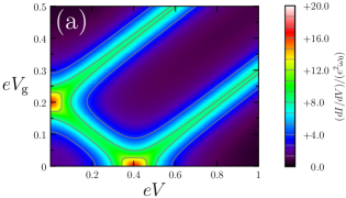
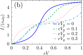
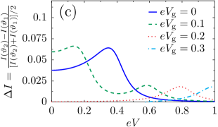
Figure 6: (Color online) Current-voltage characteristics. (a) The differential conductance $dI/dV$ is peaked when the number of levels in the current window changes at $V_{\mathrm{g}}\pm eV/2=\pm b$. (b) Obviously, the current changes when the number of level with energy between the chemical potentials of the two leads changes. (c) The level splitting $2b(\vartheta)$ depends on the orientation of the molecular spin. The relative difference of the current evaluated at the two potential minima is plotted as a function of the bias voltage. [(a) and (b) are evaluated at $\vartheta=0$. The plots are obtained with the same parameters as in Fig. 2 and all energies are measured in units of the barrier height without magnetic field $DM^{2}$.]

VI.1 Fokker-Planck equation

Our approach is based on an equivalent Fokker-Planck formulation of the Langevin dynamics of the molecular spin. We first rewrite the Langevin equation (31) for unpolarized leads. Describing the orientation of the molecular spin in terms of a polar angle $\vartheta$, measured relative to the applied magnetic field, and an azimuthal angle $\varphi$, and noting that $\dot{\mathbf{M}}/M=\dot{\vartheta}\hat{\mathbf{e}}_{\vartheta}+\dot{\varphi}\sin\vartheta\hat{\mathbf{e}}_{\varphi}$, we find the Langevin equation

$$\dot{\vartheta} =\alpha\left[M\gamma_{s,1}\sin\vartheta\,\dot{\varphi}-\delta{\cal B}_{\varphi}\right]$$

$$\sin\vartheta\,\dot{\varphi} =\alpha\bigl{[}-\partial_{\vartheta}U/M-Js_{z}\sin\vartheta+\delta{\cal B}_{\vartheta}$$

$$\qquad-M\left(\gamma_{s,1}+\gamma_{s,2}\sin^{2}\vartheta\right)\dot{\vartheta}\bigr{]},$$ (49)

where the noise correlator is given in polar coordinates by $\tilde{D}^{\varphi\varphi}=\tilde{D}^{\vartheta\varphi}=\tilde{D}_{1}$ and $\tilde{D}^{\vartheta\vartheta}=\tilde{D}_{1}+\left[(g_{e}B/2)\cos\vartheta\sin\vartheta\right]^{2}\tilde{D}_{2}$, with $\tilde{D}_{i}$ defined in Eq. (V).

Following standard procedures,zwanzig-2001 we now derive the corresponding Fokker-Planck equation for the probability distribution $P(\mathbf{M},t)$ of the magnetization vector $\mathbf{M}$ at time $t$. In the uniaxial situation under consideration, this probability distribution is independent of $\varphi$ and depends on the angle $\vartheta$ only. As outlined in Appendix B for the convenience of the reader, we then obtain the Fokker-Planck equation

$$\partial_{t}P(\vartheta,t) =\frac{1}{\sin\vartheta}\partial_{\vartheta}\sin\vartheta e^{-\tilde{V}(\vartheta)}\partial_{\vartheta}e^{\tilde{V}(\vartheta)}\tilde{\beta}(\vartheta)\,P(\vartheta,t).$$ (50)

This equation has the stationary solution $P(\vartheta)_{\mathrm{stat}}\propto\exp[{-\tilde{V}(\vartheta)}]/\tilde{\beta}$. Here we have introduced

$$\tilde{\beta}(\vartheta) =\frac{\alpha^{2}\tilde{D}_{1}/2}{1+\alpha^{2}M^{2}\gamma_{s,1}\left(\gamma_{s,1}+\gamma_{s,2}\sin^{2}\vartheta\right)},$$ (51)

and

$$\tilde{V}(\vartheta) =\int^{\vartheta}d\vartheta^{\prime}\,\frac{\partial_{\vartheta^{\prime}}U+Ms_{z}J\sin\vartheta^{\prime}}{\tilde{D}_{1}/(2\gamma_{s,1})}.$$ (52)

As long as the anisotropy is sufficiently large, $U(\vartheta)$ has a minimum $U_{1}$ at $\vartheta=\vartheta_{1}=0$, another minimum $U_{2}$ at $\vartheta=\vartheta_{2}=\pi$ and a maximum $U_{m}$ at $0<\vartheta<\pi$. We assume that this holds also for $\tilde{V}(\vartheta)$ and visualize the dependence of $\tilde{V}(\vartheta)$ on gate and bias voltage in Fig. 5. One clearly sees that the difference between the values of $\tilde{V}$ at the minima and the maximum decreases with increasing bias voltage, as one expects from the behavior of fluctuations and damping, cf. Fig. 3.

Note that in equilibrium the ratio $\tilde{D}_{1}/(2\gamma_{s,1})=T$, as dictated by the fluctuation-dissipation theorem. For zero temperature but finite bias voltages $V$ it is sometimes instructive to interpret this ratio as an effective temperature in each potential well, $T_{\mathrm{eff}}\simeq\tilde{D}_{1}/(2\gamma_{s,1})$ (as done for instance in Refs. mozyrsky-2006, ; pistolesi-2008, ; nunez-2008, ), see Fig. 3. Generally however, both coefficients, $\tilde{D}_{1}$ and $\gamma_{s,1}$ are angle dependent and non trivial functions of voltage, as we have seen explicitly above.

We calculate how long the molecular spin remains on one half of the Bloch sphere. The mean time between passing the energy barrier $\tau_{ij}$ due to the interaction with the electrons is then found by a standard procedure.zwanzig-2001 We consider an adjoint equation to Eq. (50),

$$\frac{\tilde{\beta}(\vartheta)}{\sin\vartheta}e^{\tilde{V}(\vartheta)}\partial_{\vartheta}e^{-\tilde{V}(\vartheta)}\sin\vartheta\partial_{\vartheta}\,\tau_{ij}(\vartheta)=-1/2,$$ (53)

with an absorbing boundary condition $\tau_{ij}(\vartheta_{m})=0$ in order to get the mean first passage time, as briefly outlined in Appendix B. The factor $1/2$ takes into account that it is equally likely to go to $\vartheta\gtrless\vartheta_{\mathrm{m}}$ at $\vartheta=\vartheta_{\mathrm{m}}$. Solving the equation yields

$$\tau_{12}(\vartheta)=2\int_{\vartheta}^{\vartheta_{m}}d\vartheta^{\prime}\,\frac{e^{\tilde{V}(\vartheta^{\prime})}}{\sin\vartheta^{\prime}}\int_{\vartheta_{1}}^{\vartheta^{\prime}}d\vartheta^{\prime\prime}\,\frac{\sin\vartheta^{\prime\prime}}{\tilde{\beta}(\vartheta^{\prime\prime})}e^{-\tilde{V}(\vartheta^{\prime\prime})}$$ (54)

for passing from $\vartheta<\vartheta_{m}$ to $\vartheta>\vartheta_{m}$ and an analogous expression for the opposite process.

When the potential minima are well separated and the fluctuations are small, we can give an analytical expression for the switching rate. In this limit, the integrals in (54) can be evaluated by saddle-point integration (cp. Ref. brown-1963, for the situation in which the coefficients do not depend on $\vartheta$), yielding

$$\frac{1}{\tau_{ij}}\simeq\frac{1}{\sqrt{2\pi}}\sin\vartheta_{m}\sqrt{|\tilde{V}^{\prime\prime}(\vartheta_{m})|}\tilde{\beta}(\vartheta_{i})\tilde{V}^{\prime\prime}(\vartheta_{i})e^{-[\tilde{V}(\vartheta_{m})-\tilde{V}(\vartheta_{i})]}.$$ (55)

Hence, the rate depends exponentially on the difference between $\tilde{V}$ evaluated at its maximum and minimum, respectively, so that it can be tuned by varying bias voltage and gate potential. The general behavior of $1/\tau_{ij}$, as given by Eq. (54), is shown in Fig. 5 for typical values as a function of gate and bias voltages. We discussed above that the fluctuations increase with the number of levels in the current window. This is also reflected in the fluctuation induced transition rates which increase with the bias voltage accordingly.

VI.2 Current

The current through lead $\alpha$ is given by the change of the number of particles in the lead times the electronic charge, $I_{\alpha}=-ie\langle\left[H,\sum_{k_{\alpha},\sigma}c^{\dagger}_{k_{\alpha},\sigma}c_{k_{\alpha},\sigma}\right]\rangle$. In the adiabatic limit this becomesjauho

$$I_{\alpha}=e\int\frac{d\omega}{2\pi}\mathrm{tr}\left[\left(G_{0}^{R}-G_{0}^{A}\right)\Sigma_{\alpha}^{<}+G_{0}^{<}\left(\Sigma_{\alpha}^{A}-\Sigma_{\alpha}^{R}\right)\right],$$ (56)

where $\Sigma_{\alpha}=\Sigma_{\alpha,c}$ for unpolarized leads. Noting that $I_{L}=-I_{R}=I/2$ and assuming symmetric coupling to the leads, $\Gamma_{L}=\Gamma_{R}=\Gamma/2$, we obtain, by inserting the expressions for the Green’s functions [Eqs. (63) and (65)] and the self-energies [Eqs. (60) and (20)] after straightforward algebra

$$I=\frac{e}{4\pi}\Gamma\sum_{\pm}\left[\arctan\left(\frac{\mu_{L}-\epsilon\mp b}{\Gamma/2}\right)-(L\leftrightarrow R)\right],$$ (57)

which is valid at zero temperature. As discussed above, the electronic level splits due to the interaction with the effective magnetic field $\mathbf{b}$, defined in Eq. (14). When this level splitting is larger than the level broadening $\Gamma$, the current increases as the number of levels in the transport window increases, see Fig. 1. This is reflected in peaks of the differential conductance $dI/dV$ as a function of gate and bias voltage. Note that the splitting of the electronic levels and thus the number of levels in the transport window depends on the molecular spin orientation since $b=b(\vartheta)$. As a consequence, the current is also a function of $\vartheta$. In principle, this allows one to read out the molecular switch via current measurements, see Fig. 6.

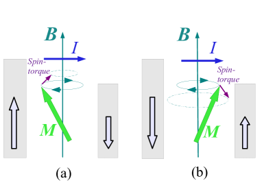
Figure 7: (Color online) Sketch of the effect of polarized leads inducing spin-torque-transfer (indicated by the magenta arrow) on the molecular moment. Depending on the polarization and the current, the spin-torque tends to align the molecular moment either (a) along or (b) against the magnetic field.

VII Spin-torque-induced switching with polarized leads

The switching mechanism discussed in the previous section originates in fluctuations of the molecular magnetic moment, introduced by the coupling to the itinerant electrons. In Sec. IV we have seen that the presence of polarized leads opens the possibility of negative Gilbert damping which could favor the switching of the molecular spin. This mechanism strongly depends on the details of the system, like the value of the mean chemical potential $\mu$ and the applied bias voltage. However, for spin-polarized leads, switching of the molecular moment under general non-equilibrium conditions will typically be dominated by a different mechanism which is driven by the non-conservative (or spin-transfer) torque exerted by the coupling to the current carrying electrons. The generic effect of the spin-torque in the dynamics of ${\bf M}$ has been reviewed in Ref. spin-torque, . This term appears already in leading order of the Born-Oppenheimer approximation in which Gilbert damping and fluctuations can be neglected.

In this section we focus on this spin-torque $-Js_{t}(\hat{\bf e}_{z}\times\hat{{\bf M}})$, see Eq. (41), in the Landau-Lifshitz-Gilbert equation (31), where $s_{t}$ is given by Eq. (43). We analyze under which microscopic conditions it is expected to drive switching in our molecular setup. In the present case it is clear that it moves the vector ${\bf M}$ along the azimuthal direction, tending to align it along the magnetic field. Thus, given a tilted molecular magnetic moment ${\bf M}$ precessing around the magnetic field, for $s_{t}<0$ the spin torque induces a spiral trajectory moving ${\bf M}$ toward orbits of smaller radius around the magnetic field. Instead, for $s_{t}>0$ it induces orbits of larger radius enabling the switching to the opposite hemisphere, with ${\bf M}$ tending to align opposite to the external magnetic field.

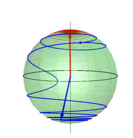
Figure 8: (Color online) Motion of the molecular moment in the presence of spin-polarized leads. For negative bias voltage $eV=-0.4$, the magnetic moment is driven toward the positive $z$ axis (red curve) while inverting the voltage $eV\rightarrow-eV$ causes a flip of the magnetic moment (blue curve). (We consider $\Gamma_{L}^{\uparrow}=\Gamma_{R}^{\downarrow}=0.1$, $\Gamma_{L}^{\downarrow}=\Gamma_{R}^{\uparrow}=0$ and $eV_{\mathrm{g}}=0$; the other parameters are the same as in Fig. 2.)

In our model, the behavior of $s_{t}$ can be rather easily analyzed in the limit of completely polarized leads, e.g. $\Gamma_{L}^{\uparrow}=\Gamma_{R}^{\downarrow}=\Gamma/2$. In this limit Eq. (43) simplifies to

$$s_{t}=-\frac{J\Gamma^{2}}{4\pi M}\int d\omega\frac{f_{L}-f_{R}}{\prod_{\pm}\left[(\omega-\epsilon\pm b)^{2}+(\Gamma/2)^{2}\right]}.$$ (58)

More generally, the sign of $s_{t}$ is determined by the condition

$$\mbox{sgn}[s_{t}]=\mbox{sgn}\left[\left(\Gamma_{L}^{\downarrow}\Gamma_{R}^{\uparrow}-\Gamma_{L}^{\uparrow}\Gamma_{R}^{\downarrow}\right)\left(f_{L}-f_{R}\right)\right].$$ (59)

Thus, when we consider a $\uparrow$-polarized left lead with $\Gamma_{L}^{\uparrow}\Gamma_{R}^{\downarrow}>\Gamma_{L}^{\downarrow}\Gamma_{R}^{\uparrow}$, a current flowing from left to right, $\mu_{L}>\mu_{R}$, results in $s_{t}<0$ and thus antialignment of magnetic moment and magnetic field. For the opposite spin-polarization, the spin-torque tends to align the magnetic moment with the magnetic field, as sketched in Fig. 7.

For a given spin-polarization, inverting the direction of the current can switch the orientation of the magnetic moment in the same way. This is studied by solving numerically the equation of motion for the molecular spin in the strictly adiabatic limit, hence neglecting Gilbert damping and fluctuations, in the presence of strongly polarized leads. In Fig. 8 we show the time evolution of the molecular spin initially slightly deviating from the magnetic field axis for two different voltages. Clearly, the motion of the molecular spin is determined by the direction of the current through the molecule, showing that inverting the bias voltage causes spin-flips in this setup.

VIII Summary and conclusions

In this work we have considered an anisotropic magnetic molecule in a single-molecule junction in which conduction electrons couple via exchange to the localized magnetic moment. The resulting current-induced torques have been analyzed by means of the non-equilibrium Born-Oppenheimer approximation, which gives rise to Langevin dynamics of the magnetic moment, described by a generalized Landau-Lifshitz-Gilbert equation. This approximation is valid in the high-current limit when the precessional frequency of the molecular spin is small compared to the electronic time scales. Unlike previous works, our approach does not follow a perturbative route either in the tunneling between leads and the molecule or in the coupling between the electronic spin and the molecular magnetic moment. Accordingly, we can render the full dependence of the parameters of the LLG equation on the state of the molecular moment as well as on the applied bias and gate voltages.

The strictly adiabatic approximation causes a mean torque exerted by the conduction electrons, while retardation effects result in a renormalization of the precession frequency and Gilbert damping. In addition, equilibrium and non-equilibrium fluctuations of the current cause a fluctuating (Langevin) torque. We have expressed these torques in terms of the electronic Green’s functions and have related them to scattering theory, in the latter case extending earlier work to include an applied bias voltage. We have concluded that in general out-of-equilibrium situations the conduction electrons can transfer energy to the localized moment by the fluctuations and, in the presence of spin-polarized leads, via a non-conservative (spin-transfer) torque and/or negative damping.

These mechanisms allow one to use the anisotropic magnetic molecule in an external magnetic field as a molecular switch which can be read out via the backaction of the molecular spin on the transport current. When the molecule is attached to metallic leads in a uniaxial setup, we have turned the Langevin equation into a Fokker-Planck equation allowing us to calculate the switching rates between the two stable spin orientations. Transitions between these states are driven by the fluctuations which we have analyzed– in addition to the mean torque, damping, and the current– as a function of the applied gate and bias voltages and the orientation of the molecular spin. In the presence of spin-polarized leads, the switching dynamics is dominated by the non-conservative (spin-transfer) part of the current-induced torque, which enables switching between the spin orientations by reversing the direction of the electronic current.

The above mentioned features of the dynamics of the local magnetic moment are also common in layered spintronic devices. However, in the present case, the different coefficients that govern the dynamics of the molecular magnetic moment show a strong dependence on the bias voltage determined by the electronic structure of the molecule (see Fig. 3). The latter property also determines the behavior of the electronic current, where features of the dynamics of the magnetic moment take place in combination with coherent tunneling of molecular systems, as signalized for instance in the current and the differential conductance (see Fig. 6).

We have considered a generic and standard model for the molecule which applies to a wide type of molecular systems, provided that a sufficiently large current flows through the molecule and that the magnetic moment is sufficiently large to fulfill the adiabatic condition assumed in the NEBO treatment. In particular, good candidates can be the Mn₁₂- or Fe₈-based devices. These systems are described by microscopic Hamiltonians of the type we considered in this work, and have rigid magnetic cores with $M=10$, and an anisotropy barrier $DM^{2}$ of the order of a few meV.fried ; revs Classical descriptions of their spin dynamics have been presented for these molecules in contact to phononic environments. zueco The crucial parameters in order to achieve the adiabatic regime in our setup, should be a good enough contact to the electrodes and a sufficiently high applied bias voltage, leading to a short dwell time of the electrons in the molecule. To be more specific, we estimate for the Mn₁₂- or Fe₈ systems with a rather large magnetic anisotropy that the Born-Oppenheimer approximation can be applied when the current through the device exceeds $\sim 10\mathrm{nA}$.

Appendix A Green’s functions, $s_{l}^{0}(t,{\bf M})$, $\gamma_{s}^{lk}(t,{\bf M})$ and noise correlator

We approximate the self-energy to be independent of energy. In this wide band limit Eq. (13) becomes

$$\Sigma_{\alpha,\sigma}^{R}(\omega) \simeq\mathrm{Re}\left(\Sigma_{\alpha,\sigma}^{R}\right)-\pi i\,\nu_{\alpha,\sigma}\left|w_{\alpha}\right|^{2}.$$ (60)

with the approximately constant density of states $\nu_{\alpha,\sigma}(\omega)\simeq\nu_{\sigma}$ and $\left|w\right|^{2}=\left(\left|w_{L}\right|^{2}+\left|w_{R}\right|^{2}\right)/2$. We introduce the abbreviations

$$\epsilon_{\sigma} = \epsilon_{0}+\sum_{\alpha}\mathrm{Re}\left(\Sigma_{\alpha,\sigma}^{R}\right)$$ (61)

$$\Gamma_{\sigma}/2 = -\mathrm{Im}\left[\Sigma_{L,\sigma}^{R}(\omega)+\Sigma_{R,\sigma}^{R}(\omega)\right]\simeq\pi\,\nu_{\sigma}\left|w\right|^{2},$$ (62)

and we will use the notation $\Sigma^{R}_{c,s}=[\Sigma^{R}_{\uparrow}\pm\Sigma^{R}_{\downarrow}]/2$ and $\Gamma_{c,s}=\sum_{\alpha}\Gamma_{\alpha,c(s)}$, with $\Gamma_{\alpha,c(s)}=(\Gamma_{\alpha,\uparrow}\pm\Gamma_{\alpha,\downarrow})/2$, taking into account possibly spin-polarized leads.

From Eq. (18) we find for the frozen retarded Green’s function

$$G_{0}^{R}(\bf{M},\omega) =\frac{1}{\tilde{\omega}^{2}-\tilde{b}^{2}}\,\left[\tilde{\omega}\,1+\mathbf{\tilde{b}}\cdot\boldsymbol{\sigma}\right]$$

$$=\frac{1}{2}\frac{1+\boldsymbol{\sigma}\cdot\mathbf{\tilde{b}}/\tilde{b}}{\tilde{\omega}-\tilde{b}}+\frac{1}{2}\frac{1-\boldsymbol{\sigma}\cdot\mathbf{\tilde{b}}/\tilde{b}}{\tilde{\omega}+\tilde{b}},$$ (63)

with $\tilde{\omega}=\left(\omega-\epsilon_{0}-\Sigma^{R}_{c}\right)\simeq\omega-\epsilon+i\Gamma_{c}/2$. Here, we include the antisymmetric part of the self-energy in the effective magnetic field,

$$\mathbf{\tilde{b}}(t)=\frac{1}{2}(J\mathbf{M}(t)+g_{e}\mathbf{B})+\Sigma^{R}_{s}\hat{\mathbf{e}}_{z}.$$ (64)

After some algebra we find the following expression for the lesser Green’s function (21):

$$G^{<}_{0}(\mathbf{M},\omega)= G_{I}^{<}(\mathbf{M},\omega)+G_{b}^{<}(\mathbf{M},\omega){\bf b}\cdot\boldsymbol{\sigma}+G_{z}^{<}(\mathbf{M},\omega)\sigma^{z}$$

$$+G_{t}^{<}(\mathbf{M},\omega)\boldsymbol{\sigma}\cdot(\hat{\mathbf{e}}_{z}\times{\bf b}),$$ (65)

where the coefficients are given by

$$G_{I}^{<}(\bf{M},\omega)= \frac{1}{|\Delta(\mathbf{M},\omega)|^{2}}\{\Sigma_{c}^{<}(\omega)[|\tilde{\omega}|^{2}+|\mathbf{\tilde{b}}|^{2}]$$

$$+\Sigma_{s}^{<}(\omega)\,2[\mbox{Re}[\tilde{\omega}]b_{z}-\frac{\Gamma_{c}\Gamma_{s}}{4}]\},$$

$$G_{b}^{<}(\bf{M},\omega)= \frac{2}{|\Delta(\mathbf{M},\omega)|^{2}}\{\Sigma_{c}^{<}(\omega)\mbox{Re}[\tilde{\omega}]+\Sigma_{s}^{<}(\omega)b_{z}\},$$

$$G_{z}^{<}(\bf{M},\omega)= \frac{1}{|\Delta(\mathbf{M},\omega)|^{2}}\{-\Sigma_{c}^{<}(\omega)\frac{\Gamma_{c}\Gamma_{s}}{2}$$

$$+\Sigma_{s}^{<}(\omega)[|\tilde{\omega}|^{2}-|\mathbf{\tilde{b}}|^{2}+\frac{\Gamma_{s}^{2}}{2}]\},$$

$$G_{t}^{<}(\bf{M},\omega)= \frac{1}{|\Delta(\mathbf{M},\omega)|^{2}}\{\Sigma_{c}^{<}(\omega)\Gamma_{s}-\Sigma_{s}^{<}(\omega)\Gamma_{c}\}.$$ (66)

We use $\Delta(\mathbf{M},\omega)=\tilde{\omega}^{2}-\tilde{b}^{2}$ and $\mathbf{\tilde{b}}\simeq\mathbf{b}-i(\Gamma_{s}/2)\hat{\mathbf{e}}_{z}$. Substituting the above expressions for $\Gamma_{c,s}$, it can be seen that $G_{t}^{<}(\mathbf{M},\omega)=0$, for $\Gamma_{L,\sigma}=\Gamma_{R,\sigma}$, implying that this component of the Green’s function contributes only for polarized leads. Note that the corresponding expressions for the larger Green’s function $G^{>}_{0}(\mathbf{M},\omega)$ are obtained by replacing $\Sigma^{<}_{c,s}$ by $\Sigma^{>}_{c,s}=-i\sum_{\alpha}\left(1-f_{\alpha}(\omega)\right)\Gamma_{\alpha,c(s)}$ in the expressions above.

Using the Green’s functions expressions, we find for the mean value of the electronic spin at the molecule

$$\mathbf{s}^{0}({\bf M})=\int\frac{d\omega}{2\pi i}\{G^{<}_{b}\mathbf{b}+G^{<}_{z}\hat{\mathbf{e}}_{z}+G^{<}_{t}(\hat{\mathbf{e}}_{z}\times{\bf b})\},$$ (67)

resulting in Eq. (40) in the case of axial symmetry. The explicit expression for the component parallel to $\mathbf{M}$ reads

$$s_{M}({\bf M}) =-\frac{iJ}{M}\int\frac{d\omega}{2\pi}G^{<}_{b}({\bf M},\omega).$$ (68)

The correction due to retardation effects associated with the slow dynamics of the molecular spin are captured by the matrix $\gamma^{lk}$, see Eq. (III.3). The symmetric part of this matrix,

$$\gamma_{s}^{lk}(\mathbf{M})=\frac{J^{2}}{4}\int\frac{d\omega}{2\pi}\mbox{tr}[\sigma^{l}\partial_{\omega}G_{0}^{>}\sigma^{k}G_{0}^{<}]_{s},$$ (69)

describes Gilbert damping of the molecular spin, induced by the coupling to the electrons. The antisymmetric part of the matrix $\gamma$ is given by

$$\gamma^{lk}_{a}(\mathbf{M}) =\frac{J^{2}}{4}\int\frac{d\omega}{2\pi}\mbox{tr}[\sigma^{l}\partial_{\omega}\left(G_{0}^{R}+G_{0}^{A}\right)\sigma^{k}G_{0}^{<}]_{a}.$$ (70)

Considering a setup with unpolarized leads and the external magnetic field pointing along the anisotropy axis, hence $\mathbf{b}=\left(J\mathbf{M}+g_{e}B\hat{\mathbf{e}}_{z}\right)/2$, Eq. (69) becomes

$$\gamma^{kl}_{s}(\mathbf{M})= \frac{J^{2}}{4}\int\frac{d\omega}{2\pi}\sum_{\alpha\beta}\frac{\Gamma_{\alpha}\Gamma_{\beta}(-\partial_{\omega}f_{\beta})}{\prod_{\pm}\left[(\omega-\epsilon\pm b)^{2}+(\Gamma/2)^{2}\right]}\delta_{kl}$$

$$+ \frac{J^{2}}{2}\int\frac{d\omega}{2\pi}\sum_{\alpha\beta}\frac{\Gamma_{\alpha}\Gamma_{\beta}(-\partial_{\omega}f_{\beta})\,(\omega-\epsilon)^{2}}{\prod_{\pm}\left[(\omega-\epsilon\pm b)^{2}+(\Gamma/2)^{2}\right]^{2}}b_{k}b_{l}.$$ (71)

This will be decomposed into a term proportional to the unit matrix and a projector onto the $z$-axis, as described in Sec. V. Note that the sign of the eigenvalues of $\gamma^{kl}_{s}$ is fixed, corresponding to damping in and out-of equilibrium. As described in the main text, the prefactor $\alpha$ in Eq. (31) is given by $\alpha(\mathbf{M})=1/\left(1+\mathbf{C}\cdot\mathbf{M}\right)$, with $\mathbf{C}$ defined in Eq. (29). This becomes

$$\mathbf{C}(\mathbf{M})=\int\frac{d\omega}{2\pi}\sum_{\alpha}\frac{J^{2}\Gamma^{2}\,\Gamma_{\alpha}f_{\alpha}\,(\omega-\epsilon)}{\prod_{\pm}\left[(\omega-\epsilon\pm b)^{2}+(\Gamma/2)^{2}\right]^{2}}\mathbf{b},$$ (72)

where we have inserted $G_{0}^{<}$, Eq. (65), and the corresponding expression for $G_{0}^{>}$ into Eq. (70).

Appendix B Fokker-Planck equation

In this appendix we derive the Fokker-Planck equation from the Langevin equation and obtain an expression for the mean first passage time, following standard arguments.zwanzig-2001

We note that the probability distribution for the molecular spin is conserved for all $t$, $\int\mathrm{d}\mathbf{M}\,f(\mathbf{M},t)=1$. Hence, we can write a continuity equation for the probability distribution,

$$\partial_{t}f(\mathbf{M},t)+\partial_{\mathbf{M}}\cdot\left(\dot{\mathbf{M}}\,f(\mathbf{M},t)\right)=0.$$ (73)

Inserting Eq. (31) for $\dot{\mathbf{M}}$ we get

$$\partial_{t}f(\mathbf{M},t)=-L\,f(\mathbf{M},t)-\partial_{\mathbf{M}}\cdot\left(\alpha\boldsymbol{\xi}(t)f(\mathbf{M},t)\right),$$ (74)

where $\boldsymbol{\xi}(t)={\bf M}\times\boldsymbol{\delta{\cal B}}$ and the differential operator $L$ is defined via its action on the function $f(\mathbf{M},t)$ as

$$L\,f =\partial_{\mathbf{M}}\cdot\left(\alpha{\bf M}\times\left[-\partial_{\mathbf{M}}U-J\mathbf{s}^{0}-\gamma_{s}\dot{\mathbf{M}}\right]f\right).$$ (75)

From this follows the implicit solution

$$f(\mathbf{M},t)= e^{-tL}f(\mathbf{M},0)$$

$$-\int_{0}^{t}\mathrm{d}t^{\prime}\,e^{-(t-t^{\prime})L}\partial_{\mathbf{M}}\cdot\left(\boldsymbol{\xi}(t^{\prime})\,f(\mathbf{M},t^{\prime})\right).$$ (76)

Inserting this again in Eq. (74) and averaging over noise, denoted by $P(\mathbf{M},t)=\langle f(\mathbf{M},t)\rangle$, yields the Fokker-Planck equation

$$\partial_{t}P(\mathbf{M},t) =-L\,P(\mathbf{M},t)+\frac{1}{2}\partial_{\mathbf{M}}\cdot(\alpha^{2}\mathbf{\tilde{D}})\cdot\partial_{\mathbf{M}}P(\mathbf{M},t)$$

$$=F\,P(\mathbf{M},t),$$ (77)

where we use that the noise is Gaussian and delta-function correlated, $\langle\xi_{k}(t)\xi_{l}(t^{\prime})\rangle=\tilde{D}^{kl}\delta(t-t^{\prime})$ and introduce the Fokker-Planck operator $F$.

We consider the distribution $P(\mathbf{M},t)$ of $\mathbf{M}$ which have been at $\mathbf{M}_{0}$ at time $t=0$ and are inside a given volume at time $t$. The mean first passage time is then given by

$$\tau(\mathbf{M}_{0})=\int dt\,t\int d\mathbf{M}\frac{-dP(\mathbf{M},t)}{dt},$$ (78)

where $-\int d\mathbf{M}\frac{dP(\mathbf{M},t)}{dt}$ is the distribution of first passage times and $\int d\mathbf{M}P(\mathbf{M},t)$ gives the number of $\mathbf{M}$ which are still in the volume of consideration at time $t$. The distribution of $\mathbf{M}$ is $P(\mathbf{M},t)=e^{tF}\delta(\mathbf{M}-\mathbf{M}_{0})$ with $P(\mathbf{M},t)=0$ when $\mathbf{M}$ is at the boundary of the volume. We insert this into Eq. (78) so that after integration by parts

$$\tau(\mathbf{M}_{0})=\int dt\int\mathbf{M}e^{tF}\delta(\mathbf{M}-\mathbf{M}_{0})=\int dte^{tF^{\dagger}}1,$$ (79)

with the adjoint Fokker Planck operator $F^{\dagger}$. This results in the differential equation

$$F^{\dagger}\tau(\mathbf{M})=-1$$ (80)

for the mean first passage time with an absorbing boundary condition.

References

- (1) M. A. Reed, C. Zhou, C. J. Muller, T. P. Burgin, and J. M. Tour, Science 278, 252 (1997); A. Nitzan and M. A. Ratner, Science 300, 1384 (2003); T. Dadosh, Y. Gordin, R. Krahne, I. Khivrich, D. Mahalu, V. Frydman, J. Sperling, A. Yacoby, and I. Bar-Joseph, Nature (London) 436, 677 (2005).
- (2) H. G. Craighead, Science 290, 1532 (2000); M. L. Roukes, Phys. World 14, 25 (2001).
- (3) M. Galperin, M. A. Ratner, and A. Nitzan, J. Phys.: Cond. Matt. 19, 103201 (2007).
- (4) H. Park, J. Park, A. K. L. Lim, E. H. Anderson, A. P. Alivisatos, and P. L. McEuen, Nature (London) 407, 57 (2000); R. H. M. Smit, Y. Noat, C. Untiedt, N. D. Lang, M. C. van Hemert, and J. M. van Ruitenbeek, ibid. 419, 906 (2002).
- (5) P. S. Cornaglia, H. Ness, and D. R. Grempel, Phys. Rev. Lett. 93, 147201 (2004); J. Koch and F. von Oppen, ibid. 94, 206804 (2005); L. Arrachea and M. J. Rozenberg, Phys. Rev. B 72, 041301 (2005).
- (6) I. Z̆utić, J. Fabian, and S. Das Sarma, Rev. Mod. Phys. 76, 323 (2004).
- (7) A. Fert, Rev. Mod. Phys. 80, 1517 (2008).
- (8) L. Bogani and W. Wernsdorfer, Nature Mater. 7, 179 (2008).
- (9) J. R. Friedman and M. P. Sarachik, Annu. Rev. Condens. Matter Phys. 1, 109 (2010).
- (10) M. Misiorny and J. Barnas, Phys. Status Solidi B 246 695 (2009); S. Sanvito, Chem. Soc. Rev. 40, 3336 (2011).
- (11) M.-H. Jo, J. E. Grose, K. Baheti, M. M. Deshmukh, J. J. Sokol, E. M. Rumberger, D. N. Hendrickson, J.R. Long, H. Park, and D. C. Ralph, Nano Lett. 6, 2014 (2006).
- (12) J. R. Friedman, M. P. Sarachik, J. Tejada, and R. Ziolo, Phys. Rev. Lett. 76, 3830 (1996); H. B. Heersche, Z. de Groot, J. A. Folk, H. S. J. van der Zant, C. Romeike, M. R. Wegewijs, L. Zobbi, D. Barreca, E. Tondello, and A. Cornia, ibid. 96, 206801 (2006).
- (13) J. Park, A. N. Pasupathy, J. I. Goldsmith, C. Chang, Y. Yaish, J. R. Petta, M. Rinkoski, J. P. Sethna, H. D. Abruña, P. L. McEuen, and D. C. Ralph, Nature (London) 417, 722 (2002); W. Liang, M. P. Shores, M. Bockrath, J. R. Long, and H. Park, ibid. 417, 725 (2002); L. H. Yu, Z. K. Keane, J. W. Ciszek, L. Cheng, J. M. Tour, T. Baruah, M. R. Pederson, and D. Natelson, Phys. Rev. Lett. 95, 256803 (2005); C. Romeike, M. R. Wegewijs, W. Hofstetter, and H. Schoeller, ibid. 96, 196601 (2006); S. Florens, A. Freyn, N. Roch, W. Wernsdorfer, F. Balestro, P. Roura-Bas, A. A. Aligia, Topical Reviews in J. Phys. Condens. Matter 23, 243202 (2011); J. J. Parks, A. R. Champagne, T. A. Costi, W. W. Shum, A. N. Pasupathy, E. Neuscamman, S. Flores-Torres, P. S. Cornaglia, A. A. Aligia, C. A. Balseiro, G. K.-L. Chan, H. D. Abruña and D. C. Ralph, Science 328, 1370 (2010) K. J. Franke, G. Schulze, J. I. Pascual, ibid. 332, 940 (2011).
- (14) A. R. Rocha, V. Garcia Suarez, S. W. Bailey, C. J. Lambert, J. Ferrer and S. Sanvito, Nature Mater. 4, 335 (2005); A. N. Pasupathy, R. C. Bialczak, J. Martinek, J. E. Grose, L. A. Donev, P. L. McEuen and D. C. Ralph, Science 306, 86 (2004).
- (15) M. Urdampilleta, S. Klyatskaya, J. P. Cleziou, M. Ruben and W. Wernsdorfer, Nature Mater. 10, 502 (2011).
- (16) O. Kahn and C. Jay Martinez, Science 279, 44 (1998); R. Ssessoli, D. Gatteschi, A. Caneschi, and M. A. Novak, Nature (London) 365, 141 (1993); W. Wernsdorfer, N. Aliaga-Alcalde, D. N. Hendrickson, and G. Christou, ibid. 416, 406 (2002).
- (17) C. Timm and F. Elste, Phys. Rev. B 73, 235304 (2006).
- (18) R. Leturcq, C. Stampfer, K. Inderbitzin, L. Durrer, C. Hierold, E. Mariani, M.G. Schultz, F. von Oppen, and K. Ensslin, Nature Phys. 5, 327 (2009).
- (19) F. Delgado, J.J. Palacios, and J. Fernández-Rossier, Phys. Rev. Lett. 104, 026601 (2010).
- (20) F. Delgado and J. Fernández-Rossier, Phys. Rev. B 82, 134414 (2010).
- (21) R.-Q. Wang, L. Sheng, R. Shen, B. Wang, and D. Y. Xing Phys. Rev. Lett. 105, 057202 (2010).
- (22) D. Mozyrsky, M. B. Hastings, and I. Martin, Phys. Rev. B 73, 035104 (2006).
- (23) F. Pistolesi, Y. M. Blanter, and I. Martin, Phys. Rev. B 78 085127 (2008).
- (24) G. Weick, F. Pistolesi, E. Mariani, and F. von Oppen, Phys. Rev. B 81, 121409(R) (2010).
- (25) G. Weick, F. von Oppen, and F. Pistolesi, Phys. Rev. B 83, 035420 (2011).
- (26) G. A. Steele, A. K. Hüttel, B. Witkamp, M. Poot, H. B. Meerwaldt, L.P. Kouwenhoven, and H. S. J. van der Zant, Science 325, 1103 (2009).
- (27) A. Naik, O. Buu, M. D. LaHaye, A. D. Armour, A. A. Clerk, M. P. Blencowe, and K. C. Schwab, Nature (London) 443, 193 (2006).
- (28) J. Stettenheim, M. Thalakulam, F. Pan, M. Bal, Z. Ji, W. Xue, L. Pfeiffer, K. W. West, M. P. Blencowe, and A.J. Rimberg, Nature (London) 466, 86 (2010).
- (29) T. N. Todorov, D. Dundas, and E. J. McEniry, Phys. Rev. B 81, 075416 (2010).
- (30) J. T. Lü, M. Brandbyge, and P. Hedegard, Nano Lett. 10, 1657 (2010).
- (31) N. Bode, S. Viola Kusminskiy, R. Egger, and F. von Oppen, Phys. Rev. Lett. 107, 036804 (2011).
- (32) N. Bode, S. Viola Kusminskiy, R. Egger, and F. von Oppen, Beilstein J. Nanotechnol. 3, 144 (2012).
- (33) H. Katsura, A. V. Balatsky, Z. Nussinov, and N. Nagaosa, Phys. Rev. B 73, 212501 (2006).
- (34) J. N. Kupferschmidt, S. Adam, and P. W. Brouwer, Phys. Rev. B 74, 134416 (2006).
- (35) J. Fransson, Phys. Rev. B 77, 205316 (2008).
- (36) A. S. Núñez and R. A. Duine, Phys. Rev. B 77, 054401 (2008).
- (37) D. M. Basko and M. G. Vavilov, Phys. Rev. B 79, 064418 (2009).
- (38) T. Dunn and A. Kamenev, Appl. Phys. Lett. 98, 143109 (2011).
- (39) C. López-Monís, C. Emary, G. Kiesslich, G. Platero, and T. Brandes, Phys. Rev. B 85, 045301 (2012).
- (40) Y. Tserkovnyak, A. Brataas, and G. E. W. Bauer, Phys. Rev. Lett. 88, 117601 (2002).
- (41) A. Brataas, Y. Tserkovnyak, and G. E. W. Bauer, Phys. Rev. Lett. 101, 037207 (2008).
- (42) A. Brataas, Y. Tserkovnyak, and G. E. W. Bauer, Phys. Rev. B 84, 054416 (2011).
- (43) K. M. D. Hals, A. Brataas, Y. Tserkovnyak, EPL 90, 47002 (2010).
- (44) J. C. Slonczweski, J. Magn. Magn. Mater. 159, L1 (1996).
- (45) L. Berger, Phys. Rev. B 54, 9353 (1996).
- (46) D. C. Ralph and M. D. Stiles, J. Magn and Magn. Mater. 320, 1190 (2008).
- (47) Y. V. Nazarov and Y. M. Blanter, Quantum Transport (Cambridge University Press, Cambridge, 2010).
- (48) H. Haug and A.-P. Jauho, Quantum Kinetics in Transport and Optics of Semiconductors (Springer, Berlin, Heidelberg, New York 2008).
- (49) M. V. Berry and J. M. Robbins, Proc. R. Soc. London, Ser. A 442, 659 (1993).
- (50) M. Moskalets and M. Büttiker, Phys. Rev. B 69, 205316 (2004).
- (51) L. Arrachea and M. Moskalets, Phys. Rev. B 74, 245322 (2006).
- (52) W. F. Brown, Phys. Rev. 130 1677 (1963).
- (53) R. Zwanzig, Nonequilibrium Statistical Mechanics (Oxford University Press, Oxford, 2001).
- (54) D. Zueco and J. L. García-Palacios, Phys. Rev. B 73, 104448 (2006).