The Impact of Circumplantary Jets on Transit Spectra and Timing Offsets for Hot-Jupiters

Abstract

We present theoretical wavelength-dependent transit light curves for the giant planet HD209458b based on a number of state of the art 3D radiative hydrodynamical models. By varying the kinematic viscosity in the model we calculate observable signatures associated with the emergence of a super-rotating circumplanetary jet that strengthens with decreased viscosity. We obtain excellent agreement between our mid-transit transit spectra and existing data from Hubble and Spitzer, finding the best fit for intermediate values of viscosity. We further exploit dynamically driven differences between eastern and western hemispheres to extract the spectral signal imparted by a circumplanetary jet. We predict that: (i) the transit depth should decrease as the jet becomes stronger; (ii) the measured transit times should show timing offsets of up to 6 seconds at wavelengths with higher opacity, which increases with jet strength; (iii) wavelength-dependent differences between ingress and egress spectra increase with jet strength; (iv) the color-dependent transit shape should vary more strongly with wavelength for stronger jets. These techniques and trends should be valid for other hot Jupiters as well. Observations of transit timing offsets may be accessible with current instrumentation, though the other predictions may require the capabilities JWST and other future missions. Hydrodynamical models utilized solve the 3D Navier-Stokes equations together with decoupled thermal and radiative energy equations and wavelength dependent stellar heating.

1 Introduction

Recent decades have witnessed an explosion of observed extrasolar planets with a wide range of physical properties. Amongst these planets, a subset transit their host star and allow for a number of new observational techniques aimed at determining interior and atmospheric composition, dayside temperature, and efficiency of energy redistribution. In addition to primary transit measurements (Charbonneau et al., 2000, eg) these tools include secondary eclipse (Deming et al., 2005, eg), differential spectroscopy (Charbonneau et al., 2002, eg), phase-curve monitoring (Harrington et al., 2006; Cowan et al., 2007, eg), Doppler absorption spectroscopy (Snellen et al., 2010), and transit spectra (Brown et al., 2002, eg).

In hopes of understanding the nature of the atmospheric dynamics and its role in both redistributing incident stellar energy throughout the atmosphere and (potentially) influencing the overall evolution of the interior, multiple groups are working on coupled radiation-hydrodynamical solutions. Multiple assumptions and approaches have been taken to both the radiative and dynamical components, including relaxation methods (i.e. Newtonian heating) (Showman & Guillot, 2002; Showman et al., 2008; Cooper & Showman, 2005, 2006; Langton & Laughlin, 2007, 2008; Menou & Rauscher, 2009; Rauscher & Menou, 2010), kinematic constraints designed to represent incident flux (Cho et al., 2003, 2008; Rauscher et al., 2008), 3D flux-limited diffusion with (Dobbs-Dixon et al., 2010) and without (Burkert et al., 2005; Dobbs-Dixon & Lin, 2008) a separate radiation component, 1D two-stream approximation (Heng et al., 2011), and 1D frequency-dependent radial radiative transfer (Showman et al., 2009). Approaches to the dynamical portion of the model have included solving the equivalent barotropic equations (Cho et al., 2003, 2008; Rauscher et al., 2008), the shallow water equations (Langton & Laughlin, 2007, 2008), the primitive equations (Showman & Guillot, 2002; Showman et al., 2008, 2009; Cooper & Showman, 2005, 2006; Menou & Rauscher, 2009; Rauscher & Menou, 2010; Heng et al., 2011), Euler’s equations (Burkert et al., 2005; Dobbs-Dixon & Lin, 2008), and the Navier-Stokes equations (Dobbs-Dixon et al., 2010).

Multiple approaches to solving this difficult problem are quite valuable. However, as observational capabilities improve we would like to begin to distinguish between different numerical approaches and parameter choices. The day-night temperature contrast from primary transit and secondary eclipse measurements and phase dependent measurements have proven useful in this respect. Many simulations listed above produce strong circumplanetary eastward equatorial jets which predict that the hottest point will be advected downwind. An analytic model for the formation of these jets by Showman & Polvani (2011) suggests that the planetary-scale temperature differential excites eddies associated with Rossby and Kelvin waves which lead to the transfer of zonal angular momentum toward the equator. Calculations of eddy angular momentum transport within the simulations presented here seem to corroborate their theory. Observations of HD189733b (Knutson et al., 2007, 2009; Agol et al., 2010) appear to have convincingly demonstrated the existence of equatorial super-rotation, showing that the hottest point in the phase curve appears slightly before secondary eclipse, as first predicted by (Showman & Guillot, 2002). However, the $3.5$-hour ($24^{\circ}$) offset of the phase variation observed at 8 microns is smaller than that predicted by General Circulation Models (GCM) with solar abundance and synchronously rotating interiors (Showman et al., 2009), which may indicate that the atmospheric velocities may have been overestimated. As GCMs are incompressible, it is possible that the velocity, which is supersonic, may have been overestimated resulting in a larger phase offset than observed. Observations of $\upsilon$-Andromeda b (Crossfield et al., 2010) indicate a much larger phase shift of $89^{\circ}$, completely out of the range of current model predictions. This large phase shift also appears at odds with the large amplitude of the phase curve (which has decreased and shifted by 90 degrees with a re-observation and re-analysis of the original data); however, the fact that this planet does not transit its host star makes it a difficult case to decipher due to the unknown mass, radius, and orbital inclination of the planet. Suffice it to say, more work is necessary before we can assemble a coherent picture of these objects.

Unfortunately, much of the detailed spatial and temporal structure that is seen in numerical simulations is hidden in the necessarily hemispherically averaged phase curves (Cowan & Agol, 2008). The phase curve can be translated into the longitudinal brightness distribution on the planet, but higher frequencies are strongly suppressed, so only coarse features may be resolved (Cowan & Agol, 2008). Temperature differences across jets, latitudinal dependence, vortices, and other interesting sub-hemisphere scale phenomena largely disappear. However, one technique that may prove quite useful in this respect is transit spectroscopy. Taken as the planet transits its host star, transit spectroscopy measures the absorption of stellar light by the upper limbs of the planetary atmosphere yielding a wavelength-dependent radius for the planet (Seager & Sasselov, 2000). Given the viewing geometry of the star, planet, and observer, such a measurement probes the meridians delineating the day and night hemispheres (the terminators). The variation in opacity with wavelength can cause the planet to vary in absorption radius by $\sim 5h$ (Burrows et al., 2003), where $h$ is the atmospheric scale-height, leading to depth variations on the order of $10R_{p}h/R_{*}^{2}\approx$0.1% for $5h\approx 3500$ km, $R_{p}\approx R_{J}$, and $R_{*}\approx R_{\odot}$.

Dynamics plays a crucial role in shaping the temperatures across the terminators both at the surface and at depth. It is here that one expects the largest deviations from radiative equilibrium. As high-velocity jets advect energy across the terminator to the nightside, the flow will cool radiatively, thus one would expect the largest nightside temperatures to be closest to the terminator. Indeed simulations show similar behavior, but the exact temperature distribution depends sensitively on the details of the flow structure and radiative and advective efficiencies. Transit spectra taken both at mid-transit and during ingress and egress have great potential to help distinguish between models and adopted parameters. Several models presented in Dobbs-Dixon et al. (2010) show pronounced variability, with the largest amplitudes at the terminator region. Targeting the terminator regions with multiple transit spectra measurements may reveal spectral changes due to such dynamically driven weather.

Several other groups have also explored the differences between transit spectra calculated with 1D or 3D models. Fortney et al. (2010) and Burrows et al. (2010) perform similar calculations utilizing the 3D GCM models of Showman et al. (2009) and Rauscher & Menou (2010), respectively. As mentioned above, the dynamical and radiative methods differ amongst these models and ours, but the method for calculating the resulting spectra from the results is largely equivalent.

In this paper we utilize the 3D pressure-temperature profiles calculated using the 3D Navier-Stokes equations coupled to wavelength-dependent stellar heating and 3D flux-limited diffusion for the re-radiated component. Models differ from Dobbs-Dixon et al. (2010) in several respects; we now allow for advective flow over the polar regions, stellar heating is modified to be both wavelength dependent and to account for the slant optical depth of stellar light, and the upper boundary condition for the radiation is improved. We describe these modifications in Section 2 along with the method for calculating transit spectra. In Section 3 we illustrate variations in the predicted transit spectra of models with varying viscosity. In essence, this is a proxy for the presence or absence of a super-rotating equatorial jet discussed above. Because the variations at mid-transit are somewhat small we also propose three methods for extracting the signal utilizing the temporally dependent transit spectra. Finally, we compare our models to existing data in the literature. We conclude in Section 4 with a discussion of the results and future detectability of such effects with the next generation of instruments.

2 Modeling Methodologies

Calculating theoretical transit spectra has been done in a number of ways, the most common of which involves a 1D solution coupling a radiative transfer routine to the assumption of vertical hydrostatic equilibrium. Here we move away from assumptions of both spherical symmetry and hydrostatic equilibrium by utilizing 3D radiation hydrodynamic models coupled together with post-processing calculations to determine the detailed wavelength dependent spectra. This allows us to produce potentially observable metrics by which we may constrain the initial 3D models. We first discuss the hydrodynamical models (particularly recent modifications to the stellar energy deposition, flow in the polar regions, and flux-limited diffusion) followed by the methods used to calculate the spectra.

2.1 3D Dynamical Modeling

To calculate the pressure and temperature throughout the atmosphere of HD209458b we utilize a fully non-linear, coupled radiative hydrodynamical code. We solve the fully compressible Navier-Stokes equations throughout the 3D atmosphere together with coupled thermal and radiation energy equations. Direct stellar heating of the planet is calculated using a fully wavelength-dependent procedure. Local 3D radiative transfer and cooling is included through multi-temperature flux-limited diffusion. This model can self-consistently produce both the radiative and dynamically induced inversions, as suggested in the observed daytime spectra (Knutson et al., 2008).

This model has been utilized to study a range of parameters, most notably the viscosity (Dobbs-Dixon et al., 2010) and opacity (Dobbs-Dixon & Lin, 2008). Imposed viscosity, beyond that which is always present in numerical simulations, is meant to represent explicit dissipation processes that may not be captured in our numerical models due to limited resolution or neglected physics. More importantly for our present discussion, it allows us to study a range of flow structures and determine how one might distinguish between them observationally.

We have implemented several important changes to the numerical model of Dobbs-Dixon et al. (2010): allowing fluid to flow over the polar regions, altering the form of the energy deposition term in the thermal energy equation, and altering the flux-limited diffusion boundary conditions. We discuss each of these changes below. Additional details regarding the hydrodynamical method can be found in Dobbs-Dixon et al. (2010).

All simulations are run with a radial, longitudinal and latitudinal resolutions of $\left(n_{r},n_{\phi},n_{\theta}\right)=\left(200,160,64\right)$. These correspond to individual grid cells of $\left(\delta r,\delta\phi,\delta\theta\right)=\left(90km,2.25^{\circ},2.8^{\circ}\right)$. Comparing to the typical pressure scale-height in Table (1) there are more then $5$ radial cells per scale-height. Typical timesteps are quite small, averaging around $10$ seconds, primarily set by radial velocity. The pressure in the simulation ranges from $10^{4}$ to $10^{-5}$ bars. Note this is much deeper then any previous simulations and includes a fully convective interior below the radiative zone traditionally simulated in irradiated planets. The important effects of convection will be discussed elsewhere.

2.1.1 Polar-Traversing Flow

In the models of Dobbs-Dixon et al. (2010), the choice of a spherical grid, coupled with finite computational resources, necessitated implementing a meridional boundary condition at high latitudes. In spherical coordinates the size of the longitudinal grid cell decreases rapidly at high latitudes. For codes requiring satisfaction of the Courant-Levy-Fredreich (CFL) condition (Courant et al., 1928) a shrinking grid size will drive the computational timestep to very low values, grinding computation to a halt. Finding a latitude that allowed significantly unencumbered flow, while not halting computation motivated the choices in Dobbs-Dixon et al. (2010).

In the results presented here we attempt to relax this condition with an approximation that allows meridional flow over the poles. Figure (1) shows a schematic of the computational region around the northpole region. We utilize a staggered grid, with velocities calculated at the appropriate cell edges and scalars defined in the center (Kley & Hensler, 1987). In our scheme, whatever flows northward from one cell immediately flows into the cell on the opposite side of the pole, this includes all meridional fluxes required for the advection scheme. In essence, each cell along the $\pm\theta_{max}$-line behaves as though the cell at $\phi=\phi+\pi$ is adjacent to it. One can choose whatever value of $\theta_{max}$ you would like. In the limit that $\theta_{max}=\frac{\pi}{2}$ the scheme is completely accurate. In deference to the CFL limitations, we take the meridional size of the polar region ($2\theta_{max}$) to be slightly larger than the $\delta\theta$ of the rest of the grid so that we may take reasonable time steps. Strictly speaking, this violates causality, as meridional flow is able to transit the entire polar region within a single timestep.

There are three reasons we believe our treatment of the pole may be justified. The first is that, to first order, we expect the model to relax to an approximately steady-state solution characterized by a large dayside driving force (incident radiation), advection of energy to the nightside (high velocity winds), nightside heating (through compression, heating, shocks, and other sources of viscosity), and finally re-radiation on the nightside (Goodman, 2009). To first order a steady-state solution is found in the models of most other groups (see Section 1 for references) including those that use other gridding techniques that do not necessitate any polar approximations. The second reason our approximation appears valid is any temporal variation that is seen in simulations is primarily confined to latitudes that are equator-ward of $\approx 60^{\circ}$. These motions are unlikely to be influenced by slightly shorter timesteps taken at the poles. Finally, the third justification of our polar treatment is a series of runs with varying $\theta_{max}$ from $70^{\circ}$ to $90^{\circ}$. Comparing the zonal (longitudinal) velocity calculated these runs we find that increasing $\theta_{max}$ widens the latitudinal extent of the zonal jet and causes a slight shift in peak velocity. However, the results appear to have largely converged by $\theta_{max}=85^{\circ}$. For the remainder of the paper we set $\theta_{max}=85.5^{\circ}$.

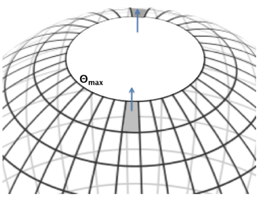
Figure 1: An illustration of the staggered grid setup near the north pole. Scalars are defined at grid centers while velocities and fluxes are defined along appropriate grid edges. Cells along the polar circle ($\left(\phi,\theta\right)=\left(\phi,\theta_{max}\right)$) utilize the cell at $\left(\phi+\pi,\theta_{max}\right)$ as a neighboring cell. For instance, the two shaded cells communicate directly and the velocities (blue arrows) across the cell edges are identical.

2.1.2 Wavelength-Dependent Stellar Energy Deposition

We have significantly improved the method by which we calculate where the stellar energy is deposited into the upper atmosphere by utilizing a wavelength-dependent prescription rather then a gray approach. Following Showman et al. (2009), we divide the spectra into $30$ wavelength bins (see Showman et al. (2009) Table 1 for a list of the bin boundaries) and calculate the opacity within each bin independently. We then calculate the spatial distribution of energy deposition in each of these bins and sum over all bins to get the net energy deposition at each location. The equation for the thermal energy can be written as

$$\left[{{\partial\epsilon}\over{\partial t}}+({\bf u}\cdot\nabla)\epsilon\right]=-P\nabla\cdot{\bf u}-\rho\kappa_{P}\left[B\left(T\right)-cE_{R}\right]$$ (1)

$$+D_{v}+\left(\frac{R_{\star}}{a}\right)^{2}\rho\sum_{b=1}^{30}\pi B\left(T_{\star}\right)_{b}\kappa_{b}e^{-\tau_{b}/\mu}\Delta\nu.$$

The second term on the left represents the advection of thermal energy and the terms on the right are the work done by compression, the exchange of energy between matter and radiation, viscous heating, and the direct heating by incident stellar irradiation, respectively. Note that we have also added a $\mu=\cos\left(\theta_{\star}\right)$, where $\theta_{\star}$ is the angle between the local normal and the incident radiation. This accounts for the additional material stellar photons encounter when traversing the limb of the planet (For a more detailed description of the derivation of this equation and the radiation energy equation see Dobbs-Dixon et al. (2010)).

In Figure (2) we show the behavior of the last term in Equation (2.1.2) at the sub-stellar point. The upper panel illustrates heating as a function of both depth and wavelength, while the lower panel shows the sum over all the wavelength bins. We find that the distribution and overall magnitude of energy deposition using this binning method matches a full wavelength-dependent calculation quite well. When compared to the gray approach of Dobbs-Dixon et al. (2010), we find the region of energy deposition is somewhat more extended. Regions of the spectra with low opacity (near $3\mu m$ for example) are able to penetrate further into the atmosphere.

Figure 2: The behavior of the stellar energy deposition term $\left(\frac{R_{\star}}{a}\right)^{2}\pi B_{b}\left(T_{\star}\right)\rho\kappa_{b}e^{-\tau_{b}/\mu}\Delta\nu$ from Equation (2.1.2) at the substellar point for each wavelength bin (upper panel) and as summed over all bins (lower panel).

2.1.3 Flux-Limited Diffusion Boundary Conditions

The classic form of flux-limited diffusion (FLD) (Levermore & Pomraning, 1981) postulates that the radiative flux can be written as ${\bf F}=-\lambda c/\left(\rho\kappa_{R}\right)\nabla E_{R}$, where $\lambda$ is a temporally and spatially variable flux limiter providing the closure relationship between flux and radiation energy density. It is typically formulated to give limits for flux in the optically-thick regime, ${\bf F}=-4acT^{3}/\left(3\rho\kappa_{R}\right)\nabla T$, and the optically-thin regime, $|{\bf F}|=cE_{R}$.

The problem lies in the application of the free-streaming, optically-thin limit to planetary atmospheres. The free-streaming limit assumes that all of the radiation is collimated and moving in the outward direction at $\tau=0$. Thus, by conservation of energy, $E_{R}=Fc$, i.e. the energy density in any given cell is determined by the rate at which radiation flows through that cell, assuming Cartesian geometry.

However, this is not the limit we are in at the photosphere of the planet. Since limb-darkening of the planet is weak, an observer placed close to $\tau=0$ near the surface of the planet will see thermal radiation that is nearly isotropic from $2\pi$ steradians towards the planet and no thermal radiation from the opposite hemisphere. Therefore, the free-streaming limit does not apply close to the planet. Instead, we must consider the energy density and flux given the non-isotropic intensity. The energy density is the first moment of the intensity and can be written $E_{R}=\int_{2\pi}I_{0}d\Omega=2\pi I_{0}$. The flux is simply the second moment and can be expressed as $F=c\int_{2\pi}I_{0}\mu d\Omega=c\pi I_{0}$. Comparing these expressions we see that the proper relation between energy density and flux at the boundary should be $F\sim cE_{R}/2$. A given flux, set by the sum of the incident and internal flux, will result in a larger energy density, and equivalently a higher temperature.

2.2 Radiative Transfer

To determine the transit spectra of HD209458b models, we calculate the wavelength dependent absorption of stellar light traversing through the limb of the planet. This allows us to determine the effective radius of the planet and a fractional reduction of stellar flux $F_{\star}$. Neglecting limb-darkening of the star, this can be expressed as

$$\left(\frac{F_{in-transit}}{F_{\star}}\right)_{\lambda}=\frac{\int\left(1-e^{-\tau\left(b,\alpha,\lambda\right)}\right)bdbd\phi}{\pi R_{\star}^{2}},$$ (2)

where $\tau\left(b,\alpha,\lambda\right)$ is the total optical depth along a given chord with impact parameter b and polar angle $\alpha$, defined on the observed planetary disk during transit. The density and temperature needed to calculate $\tau$ at each location are interpolated from the values in the 3D models.

Wavelength-dependent opacities are taken from the atomic and molecular opacity calculations of Sharp & Burrows (2007). These calculations neglect the effects of grains on absorption, assuming that grains will rain out of the upper atmosphere before they grow to any significant size.

3 Calculated Transit Spectra

In this section we present transit spectra calculated from 3D radiative-hydrodynamical models exploring the different flow structures among models with varying viscosity. While several features may influence the transit spectra at precisions already observed, others must await the next generation of instruments (as discussed in the conclusion). We highlight three methods for extracting this signal from actual data, exploiting the differences between transit spectra taken during transit ingress and egrees. We show that the time dependence of the transit signal can be used to extract information about the eastern and western hemispheres.

3.1 Varying Viscosity

The source of viscosity in the atmospheres of irradiated giant planets is a major outstanding issue (Li & Goodman, 2010) and can play an important role in shaping the overall structure of the atmospheric dynamics and energy re-distribution. Physically motivated sources of viscosity can arise from both unresolved process (sub-grid effects) or missing physics (e.g. magnetic viscosity as discussed by Batygin & Stevenson (2010) and Perna et al. (2010)). Unresolved processes may include the generation of turbulence through shocks, instabilities, or waves. Numerical viscosity, present in all numerical simulations, may also allow flow to smoothly traverse additional shocks throughout the simulation. Such shocks may, if resolved, act as an additional source of viscosity converting the kinetic energy of the jet to thermal energy that can be subsequently radiated away.

To explore the role of an isotropic viscosity disregarding its potential origin, Dobbs-Dixon et al. (2010) performed a series of simulations with varying kinematic viscosity ($\nu$). We have revisited these models allowing for the cross-pole flow as described in Section (2.1.1), wavelength-dependent heating (2.1.2), an improved FLD boundary condition (2.1.3), and significantly higher spatial resolution. Transit spectra calculated from our models during mid-transit are shown in Figure (3). The variations due to varying flow structures (See Figures (2) and (3) of Dobbs-Dixon et al. (2010) for an illustration of the differences) can be quite dramatic, including a transition from subsonic to supersonic wind speeds as the viscosity is lowered. Table (1) gives a summary of the simulation parameters.

Simulation	$\nu$ ($\mathrm{cm^{2}/s}$)	$\alpha_{eff,ph}$	$H_{ss,P}$ (km)	peak $v_{\phi}$ (km/s)
$S1$	$10^{12}$	$10^{-1}$	538	0.76
$S2$	$10^{11}$	$10^{-2}$	501	1.48
$S3$	$10^{10}$	$10^{-3}$	489	3.70
$S4$	$10^{9}$	$10^{-4}$	481	4.90
$S5$	$10^{8}$	$10^{-5}$	461	4.82

Table 1: Values of kinematic viscosity used for the simulations presented here. For reference we also quote an average effective alpha-parameter, sub-stellar pressure scale-height at the photosphere, and peak zonal velocities, increasing with decreasing viscosity.

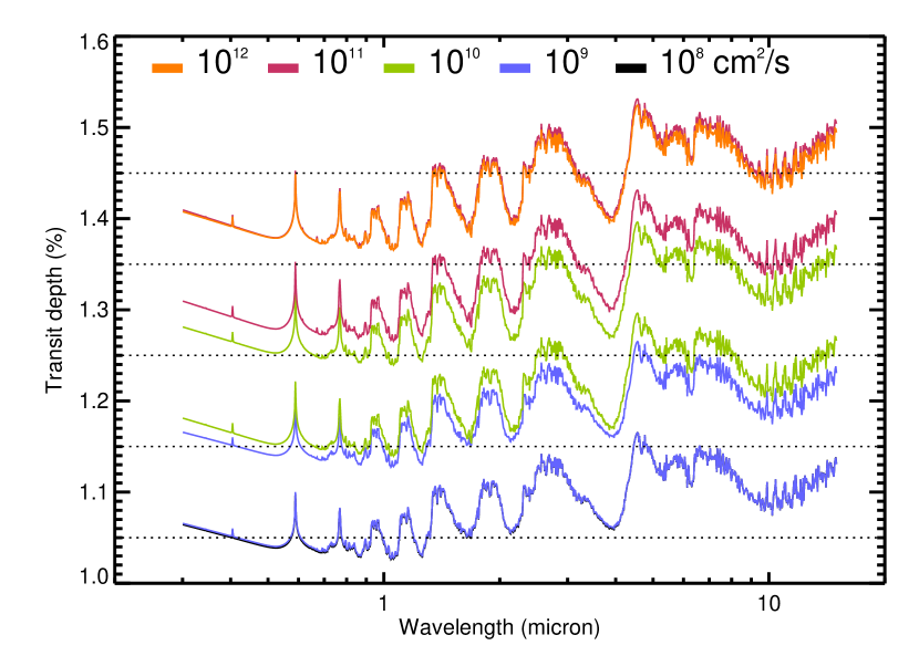
Figure 3: Difference in mid-transit transit spectra among models with varying viscosity. Successive pairs of spectra, with decreasing viscosities, are shifted downward $0.1\%$ for clarity. The reference dotted lines are similarly offset.

The transit spectra shown in Figure (3) illustrate a number of interesting features. Common to all spectra are broad absorption features due primarily to H₂O, CH₄, and CO, strong narrow features due to Na and K, and a rising signal at short wavelengths associated with Rayleigh scattering. The highest viscosity simulation has the largest overall transit depth at all wavelengths. The overall transit depth decreases roughly monotonically with decreasing viscosity, though spectra for the two highest and two lowest viscosities are virtually indistinguishable.

The trend of increasing transit depth with viscosity can be understood by examining the transition in the dynamics as viscosity is decreased. The highest viscosity simulations significantly restricts advection across the terminators. This results in symmetric flow across the eastern and western terminators, both with average scale-heights of approximately $450$ km. The zonal flow is subsonic and dies out soon after crossing the terminator. However, as the viscosity is decreased a super-rotating jet develops that circumnavigates the entire planet. This fundamentally changes the temperature of the advected gas across the terminators. For the high-viscosity simulations, the flow across both terminators is advecting gas from day to night. For the lowest viscosity simulation, the circumplanetary jet implies that the flow is still advecting gas from day to night at the eastern terminator (defined relative to the sub-stellar point), but from night to day at the western terminator. This results in scale-heights of $440$ km at the eastern terminator, but only $340$ km at the western terminator (we exploit this difference in the next sub-sections). Mid-transit spectra represent the average of the two, leading to larger overall transit depths for high-viscosity simulations.

The transition from symmetric to antisymmetric flow patterns can also be understood within the context of the work of Showman & Polvani (2011). The transport of angular momentum up-gradient to form an equatorial super-rotating circumplanetary jet is achieved primarily horizontally through eddies that have northwest/southeast (southwest/northeast) phase tilt in the northern (southern) hemisphere. The result is that eddies in both hemispheres transfer eastward angular momentum toward the equator and westward angular momentum to higher latitudes. We have performed eddy-analysis on our results utilizing the formalism of Karoly et al. (1998) and confirm that meridional eddies are the dominate source of the equatorial jet’s angular momentum. The primary excitation of these eddies are zonally propagating planetary-scale (Rossby and Kelvin) waves. High-viscosity simulations effectively inhibit the propagation of these waves and their associated eddies and thus preclude the formation of super-rotating circumplanetary jets.

3.2 Extracting the Transit shape

For number of reasons, including rotation (Seager & Hui, 2002; Barnes & Fortney, 2003), strong zonal winds (Barnes et al., 2009), equator-pole temperature gradients, and the tidal potential of the host star (Leconte et al., 2011) short period, synchronously rotating, irradiated planets are not spherical. In order to explore these variations we illustrate the shape of the planet at $4.422$ and $3.904\mu m$ in the black curve of Figure (4) for the simulation with the lowest viscosity ($10^{8}\mathrm{cm^{2}/s}$). As can be seen in Figure (3), these two wavelengths were chosen to have the largest ($4.422\mu m$) and smallest ( $3.904\mu m$) transit light depths for wavelengths shortward of $10\mu m$. This implies that $3.904\mu m$ observations will probe much deeper into the atmosphere where the planet becomes more spherically symmetric. Higher in the atmosphere at $4.422\mu m$, there are significant discrepancies between the mean surface (shown in red) and the photosphere, illustrating the dominant role of energy redistribution in determining the detailed shape of the planet. Below, we use this fact to justify extracting detailed temperature distributions from variations in the planetary shape with wavelength.

Also shown in Figure (4) is the geopotential surface (in blue) corresponding to the mean radius (in red). The geopotential combines the gravity and centrifugal forces into a single potential $\nabla Q=1/2\nabla\left({\bf\Omega}\times{\bf r}\right)^{2}+\nabla\Phi$. For a slow rotating planet such as HD209458b the temperature gradients across the planet (yielding varying scale-heights) are the largest factor in changing the planets shape. This can be seen most clearly at $3.904\mu m$ where, despite having the least amount of asymmetry, the oblateness caused by scale-height changes (black line) exceeds the rotational oblateness of the planet (red line).

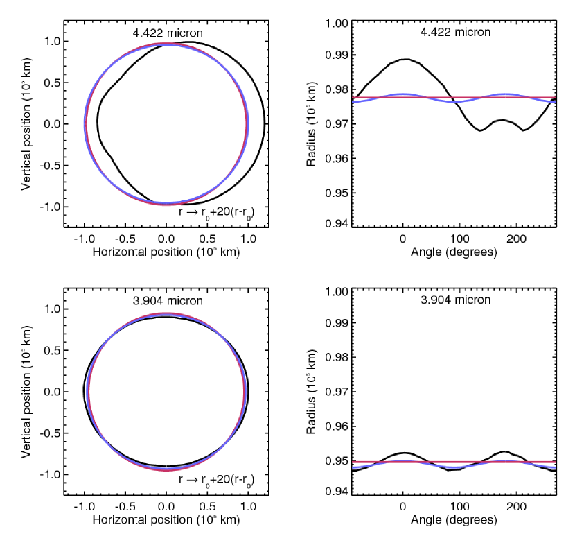
Figure 4: The wavelength dependent shape of the planet at $4.422\mu m$ (top row) and $3.904\mu m$ (bottom row) for the $\nu=10^{8}$ cm² s^-1 simulation. The left column shows the shape of the planet as seen during transit. The black curves illustrates the actual planetary shape (where $\tau\left(\lambda\right)=2/3$), the red curve illustrates a spherical planet, and the blue curve illustrates a planet filling a Roche-potential (both normalized to have the same total area). The planet shape has been exaggerated by a factor of 20 in the left column. The right column shows the same quantities as a function of latitude along the day-night delineator. An angle of $0$ corresponds to the equator and $\pi/2$ to the northpole.

Because the planet’s absorption cross-section is oblate, due primarily to the high temperatures, we can utilize observational information of the transit shape to study the efficiency of dynamical redistribution of energy throughout the atmosphere. In addition to the equator-pole differences, in models with low viscosity that have strong super-rotating recirculation, the eastern terminator has at a higher temperature than the western, and thus has a larger scale-height, so the eastern hemisphere presents a larger absorption cross-section than the western hemisphere. This is also evident in the black curve of Figure (4). Consequently, the planet has an asymmetric egg-shaped absorption cross-section which directly translates into an asymmetry in the transit shape. In the remainder of this subsection we present three methods for diagnosing this observationally: wavelength-dependent transit timing, differences between ingress and egress spectra, and color-dependent transit shape.

The first method we discuss is wavelength-dependent transit timing. Since the western terminator has a smaller scale-height and this part of the planet transits first, the ingress will be slightly delayed, while the eastern terminator is more extended, causing the end of ingress to be delayed. Likewise, the egress will be delayed as well, so the overall shift will be delay the transit relative to the center of mass of the planet. At wavelengths with larger opacity this asymmetry is stronger so the transit time delay is larger, while at wavelengths with smaller opacity it is weaker; consequently, the central time of transit will appear to vary with wavelength if one fits the transit with a symmetric planet model. Figure 5 shows the effective transit time offset versus wavelength computed for a model with no limb-darkening for the star and by fitting the transit at each wavelength with a circular planet model (Mandel & Agol, 2002). As the viscosity grows, the two hemispheres have smaller temperature differences, and hence, the transit shape is more symmetric, causing a smaller time offset.

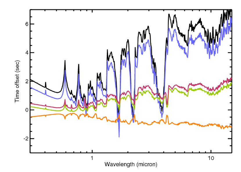
Figure 5: Effective time offset versus wavelength derived by forcing a circular fit to the planetary shape. Timing variations are primarily due to differences in the temperature structure between eastern and western terminators. Colors represent simulations with varying viscosities as in Figure (3).

A second means of diagnosing the difference between the hemispheres is to flip the light curve about the midpoint and subtract it from the original. The deviations that remain show the difference between the ingress and egress caused by a difference in shape of the east and west terminators, in addition to the time offset. To characterize this, we compute the maximum value of this deviation for each light curve computed at a specific wavelength. Figure 6 shows this maximum deviation versus wavelength. To compute this, we calculate the maximum of the absolute value of the lightcurve minus the time-reversed light curve. The largest deviations are at the $10^{-4}$ level for wavelengths dominated by water absorption opacity, and these deviations grow as the viscosity decreases due to the larger differences between the terminators for smaller viscosity. In practice, finding the midpoint of the transit around which to flip the light curve is not straightforward. As noted by Barnes et al. (2009), as transit photometry is sensitive to the shape of the planet and not the center of mass, the offset between the two cannot be determined ab initio. However, observing at multiple wavelengths, one may utilize the wavelength with the smallest transit depth to define the center of transit with the understanding that this is probing the deepest, most spherically symmetric region in the planet. This is illustrated in Figure (4).

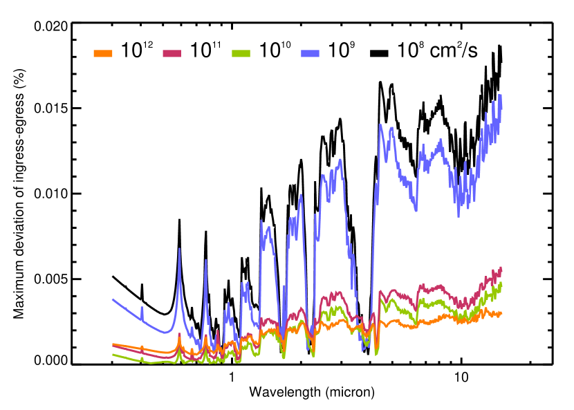
Figure 6: Maximum deviation between the ingress and egress spectra. To calculate these curves we subtract the absolute value of the lightcurve from the same lightcurve time-reversed about the central time of transit.

Finally, a third, model-independent diagnostic for the planet asymmetry is the color-dependent transit shape. Figure 7 shows the difference in the shape of transit for two wave bands: 1.55-1.70 and 2.4-3.1 micron, corresponding to the proposed JWST NIRCam F162M and F277W filters, respectively. To compute the shape difference, we subtract the two lightcurves after renormalizing the depth of the second to match the depth of the first. This model-independent measurement of the difference in the shape of the transit in these two wave-bands can be written as $C=(D_{1}-D_{2}D_{1,max}/D_{2,max})$ where $D_{1,2}$ are the depths of transit (in dimensionless units the out-of-transit flux minus the in-transit flux divided by the out-of-transit flux) and the max subscript indicates the maximum depth of transit. The asymmetry in these lightcurves clearly demonstrates that at different wavelengths the planet absorbs with a different asymmetric cross section. These filters have several advantages; they can be observed simultaneously with JWST using the dichroic and the two bands are centered at wavelengths with high and low water opacity, respectively, yielding a larger differential signal.

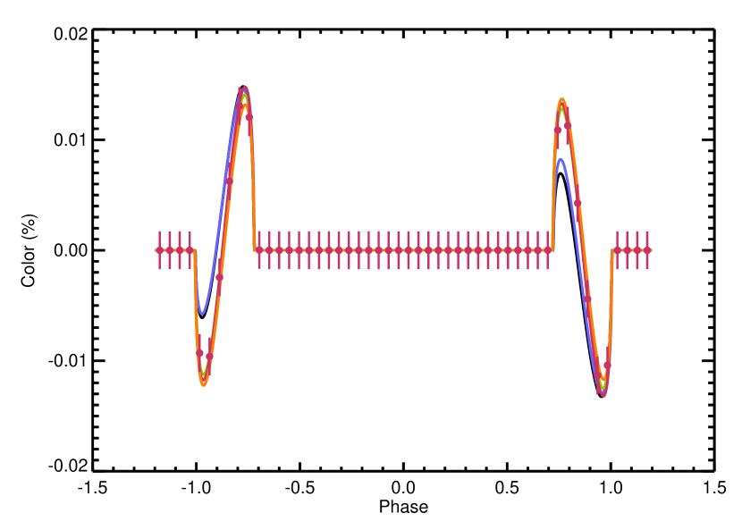
Figure 7: Color of transit for the F162M minus the re-normalized F277W JWST NIRCam filters. Vertical bars indicate predicted errors for NIRCam.

3.3 Comparison to observations

As a check on the total depth of transit, we have compared the transit depth to observations by Knutson et al. (2008) and Beaulieu et al. (2010). These observations cover wavelengths from $0.3$ to $10$ microns, and thus provide an important validation test of these numerical models. We have averaged the models over the observed bands, and have varied the value of the inner radius of the simulation zone to obtain the best agreement with the observed transit depths. This is not as accurate as carrying out additional simulations in which the model region is varied; however, this would be much more computationally expensive. Furthermore, the assumption of constant g in both these simulations and those of all other groups allows for such a shift as only the curvature terms are affected. The applied depth offset is quite small, amounting to a maximum correction of only a $1\%$ to the planetary radius. Finally, we exclude the bands with strong sodium and potassium absorption as there is evidence that potassium is depleted (which is not accounted for in our opacity tables).

There are twelve wave bands that we use, and with one free parameter, gives eleven degrees of freedom for each model. Figure 8 shows the comparison of the models to the data. We find best-fit $\chi^{2}$ of $25.41$, $25.04$, $37.62$, $45.73$, and $38.77$ for the models with viscosities of $10^{8},10^{9},10^{10},10^{11}$ and $10^{12}$ cm² s^-1 respectively. Qualitatively, the overall agreement of the models with the data is quite good: (1) the transit depth is weakly dependent on the viscosity; (2) there are no discrepancies between the data and model greater than $2-\sigma$; (3) the observed transit spectrum with wavelength shows the expected features due to water and Rayleigh scattering. In general, the success of this model is comparable to transit spectra calculated from other models which utilize GCM simulations (Fortney et al., 2010; Burrows et al., 2010).

However, in detail there are significant discrepancies; in particular, the observed IRAC transit depths appear to vary more strongly with wavelength than the model predicts. This is reflected in the larger $\chi^{2}$ of the fits, of which one-half to two-thirds is due to the infrared discrepancies. The fit to the infrared data obtained by Beaulieu et al. (2010) has an extremely good $\chi^{2}$; however, their model was one-dimensional, and allowed the abundances and temperature/pressure profile to float, so it is not surprising that they obtain a good fit with so many degrees of freedom. Another possibility is that systematic errors still exist in the IRAC data reduction. For example, for the transiting planet HD 189733b, different groups have obtained markedly different transit depths at infrared wavelengths using the same IRAC data sets; consequently, there may be some remaining systematic error present in the data (Désert et al., 2009). The final possibility is that there is still physics that is not included in our models which is causing the discrepancies; for example, varied chemical abundances, non-equilibrium chemistry, and magnetic drag have not been included in these models.

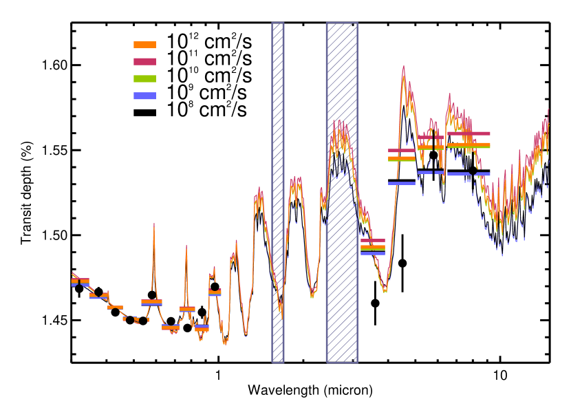
Figure 8: Transit depth versus wavelength. The black dots with error bars are the data from Knutson et al. (2007) and Beaulieu et al. (2010). The thick horizontal bars are the four models averaged over the measured wave bands. The curves show model spectra binned by a factor of 10 in wavelength.

4 Discussion

In this paper we have presented wavelength-dependent transit spectra for a series of simulations utilizing a state of the art, 3D radiative hydrodynamical model. The simulations presented here have been updated from Dobbs-Dixon et al. (2010) to allow for flow over the polar regions, wavelength-dependent stellar energy deposition which accounts for the slant optical depth, and an improved boundary condition for flux-limited diffusion. By ‘observing’ these simulations we are able to explore potentially detectable diagnostics of the overall state of the atmospheric dynamics.

We have explored the role of changing viscosity on the observable transit spectra. Larger viscosity (potentially caused by unresolved instabilities, shocks, magnetic fields, etc.) significantly alters the overall flow structure. These changes lead to variations in the observed transit spectra during the center of primary transit, but are much more evident in differential spectral measurements. We explore three separate methods to detect such variation: wavelength-dependent transit timing, differences in absorption between ingress and egress, and color-dependent transit shape. We also explored the the observable variations in transit spectra due to exo-weather. Dobbs-Dixon et al. (2010) identified dynamically-induced variation in their intermediate viscosity simulation. Based on these results and the range of observational evidence both for and against variability (Grillmair et al., 2008; Agol et al., 2010) we found sufficient motivation to look for signatures of variability. However, we find that the observable variations in transit spectra due to exo-weather are somewhat limited and likely undetectable, even with JWST. However, one final note of caution is in order. The weather related phenomena we explore are limited to dynamically induced variations. Chemically-induced variations due to clouds, non-equilibrium chemistry, etc. may potentially couple positively to dynamical variations and amplify the observability of exo-weather.

We have compared our analytical results for simulations with varying viscosity to the observations of HD209458b by Knutson et al. (2007) and Beaulieu et al. (2010). In general, we find quite good agreement, with none of the discrepancies greater then $2-\sigma$. Overall, our best fit model is the simulation with viscosity set to $10^{9}\mathrm{cm^{2}/s}$, which has developed a super-rotating circumplanetary jet at the equator. The largest differences between our models and the observations occur in the IR where we find that we consistently over-predict the transit depth in the observed $3.6$ and $4.5\mu m$ IRAC bands. Fortney et al. (2010) and Burrows et al. (2010) have performed an analysis similar to ours utilizing GCM dynamical models. They find disagreements with the IRAC bands as well, over-predicting the shorter bands and under-predicting the longer IRAC bands. Shabram et al. (2011) also discusses difficulties matching the models of Beaulieu et al. (2010) to analytic models of Lecavelier Des Etangs et al. (2008).

Although the measurements presented here are likely beyond our current capabilities it is informative to speculate on future possibilities. The quoted error bars in Beaulieu et al. (2010) are $0.013$, $0.017$, $0.015$ and $0.011$ for the four IRAC wavebands (with increasing $\lambda$). The James Webb Space Telescope (JWST) will have approximately $43$ times the collecting area of the Spitzer telescope. Assuming that the S/N is photon-limited, this will yield errors for the full transit that are $6.6$ times smaller. A similar measurement would thus have errors of approximately $0.0022\%$. Given the results presented here, distinguishing between models with varying viscosity is potentially accessible to JWST observations.

Utilizing the difference between ingress and egress spectra through one of the methods described here remains the most viable mechanism to distinguish between dynamical models. Errors in this measurement increase due to the decreased time of observation. Ingress or egress would be shorter than the transit duration by $\frac{R_{p}}{2R_{\star}}\frac{1}{1-b^{2}}\approx 0.08$, where $b$ is the impact parameter of the orbit. This gives total errors in a JWST measurement of the order of $0.0076$. Figure (6) shows wavelength-dependent deviations are detectable given this level of error. The color dependent transit light curve shown in Figure (7) explicitly shows the expected error, again illustrating the clear detectability of this signal.

References

- Agol et al. (2010) Agol, E., Cowan, N. B., Knutson, H. A., et al. 2010, ApJ, 721, 1861
- Barnes et al. (2009) Barnes, J. W., Cooper, C. S., Showman, A. P., & Hubbard, W. B. 2009, ApJ, 706, 877
- Barnes & Fortney (2003) Barnes, J. W. & Fortney, J. J. 2003, ApJ, 588, 545
- Batygin & Stevenson (2010) Batygin, K. & Stevenson, D. J. 2010, ArXiv e-prints
- Beaulieu et al. (2010) Beaulieu, J. P., Kipping, D. M., Batista, V., et al. 2010, MNRAS, 409, 963
- Brown et al. (2002) Brown, T. M., Libbrecht, K. G., & Charbonneau, D. 2002, PASP, 114, 826
- Burkert et al. (2005) Burkert, A., Lin, D. N. C., Bodenheimer, P. H., Jones, C. A., & Yorke, H. W. 2005, ApJ, 618, 512
- Burrows et al. (2010) Burrows, A., Rauscher, E., Spiegel, D. S., & Menou, K. 2010, ApJ, 719, 341
- Burrows et al. (2003) Burrows, A., Sudarsky, D., & Hubbard, W. B. 2003, ApJ, 594, 545
- Charbonneau et al. (2000) Charbonneau, D., Brown, T. M., Latham, D. W., & Mayor, M. 2000, ApJ, 529, L45
- Charbonneau et al. (2002) Charbonneau, D., Brown, T. M., Noyes, R. W., & Gilliland, R. L. 2002, ApJ, 568, 377
- Cho et al. (2003) Cho, J. Y.-K., Menou, K., Hansen, B. M. S., & Seager, S. 2003, ApJ, 587, L117
- Cho et al. (2008) —. 2008, ApJ, 675, 817
- Cooper & Showman (2005) Cooper, C. S. & Showman, A. P. 2005, ApJ, 629, L45
- Cooper & Showman (2006) —. 2006, ApJ, 649, 1048
- Courant et al. (1928) Courant, R., Friedrichs, K., & Lewy, H. 1928, Mathematische Annalen, 100, 32
- Cowan & Agol (2008) Cowan, N. B. & Agol, E. 2008, ArXiv e-prints
- Cowan et al. (2007) Cowan, N. B., Agol, E., & Charbonneau, D. 2007, MNRAS, 379, 641
- Crossfield et al. (2010) Crossfield, I. J. M., Hansen, B. M. S., Harrington, J., et al. 2010, ApJ, 723, 1436
- Deming et al. (2005) Deming, D., Seager, S., Richardson, L. J., & Harrington, J. 2005, Nature, 434, 740
- Désert et al. (2009) Désert, J.-M., Lecavelier des Etangs, A., Hébrard, G., et al. 2009, ApJ, 699, 478
- Dobbs-Dixon et al. (2010) Dobbs-Dixon, I., Cumming, A., & Lin, D. N. C. 2010, ApJ, 710, 1395
- Dobbs-Dixon & Lin (2008) Dobbs-Dixon, I. & Lin, D. N. C. 2008, ApJ, 673, 513
- Fortney et al. (2010) Fortney, J. J., Shabram, M., Showman, A. P., et al. 2010, ApJ, 709, 1396
- Goodman (2009) Goodman, J. 2009, ApJ, 693, 1645
- Grillmair et al. (2008) Grillmair, C. J., Burrows, A., Charbonneau, D., et al. 2008, Nature, 456, 767
- Harrington et al. (2006) Harrington, J., Hansen, B. M., Luszcz, S. H., et al. 2006, Science, 314, 623
- Heng et al. (2011) Heng, K., Frierson, D. M. W., & Phillipps, P. J. 2011, ArXiv e-prints
- Karoly et al. (1998) Karoly, D. J., Vincentt, D. G., & Schrage, J. M., eds. 1998, General Circulation. Meterology of the Southern Hemisphere, Vol. 27
- Kley & Hensler (1987) Kley, W. & Hensler, G. 1987, A&A, 172, 124
- Knutson et al. (2008) Knutson, H. A., Charbonneau, D., Allen, L. E., Burrows, A., & Megeath, S. T. 2008, ApJ, 673, 526
- Knutson et al. (2007) Knutson, H. A., Charbonneau, D., Allen, L. E., et al. 2007, Nature, 447, 183
- Knutson et al. (2009) Knutson, H. A., Charbonneau, D., Cowan, N. B., et al. 2009, ApJ, 690, 822
- Langton & Laughlin (2007) Langton, J. & Laughlin, G. 2007, ApJ, 657, L113
- Langton & Laughlin (2008) —. 2008, ApJ, 674, 1106
- Lecavelier Des Etangs et al. (2008) Lecavelier Des Etangs, A., Vidal-Madjar, A., Désert, J., & Sing, D. 2008, A&A, 485, 865
- Leconte et al. (2011) Leconte, J., Lai, D., & Chabrier, G. 2011, A&A, 528, A41+
- Levermore & Pomraning (1981) Levermore, C. D. & Pomraning, G. C. 1981, ApJ, 248, 321
- Li & Goodman (2010) Li, J. & Goodman, J. 2010, ApJ, 725, 1146
- Mandel & Agol (2002) Mandel, K. & Agol, E. 2002, ApJ, 580, L171
- Menou & Rauscher (2009) Menou, K. & Rauscher, E. 2009, ApJ, 700, 887
- Perna et al. (2010) Perna, R., Menou, K., & Rauscher, E. 2010, ArXiv e-prints
- Rauscher & Menou (2010) Rauscher, E. & Menou, K. 2010, ApJ, 714, 1334
- Rauscher et al. (2008) Rauscher, E., Menou, K., Cho, J. Y.-K., Seager, S., & Hansen, B. M. S. 2008, ApJ, 681, 1646
- Seager & Hui (2002) Seager, S. & Hui, L. 2002, ApJ, 574, 1004
- Seager & Sasselov (2000) Seager, S. & Sasselov, D. D. 2000, ApJ, 537, 916
- Shabram et al. (2011) Shabram, M., Fortney, J. J., Greene, T. P., & Freedman, R. S. 2011, ApJ, 727, 65
- Sharp & Burrows (2007) Sharp, C. M. & Burrows, A. 2007, ApJS, 168, 140
- Showman et al. (2008) Showman, A. P., Cooper, C. S., Fortney, J. J., & Marley, M. S. 2008, ApJ, 682, 559
- Showman et al. (2009) Showman, A. P., Fortney, J. J., Lian, Y., et al. 2009, ApJ, 699, 564
- Showman & Guillot (2002) Showman, A. P. & Guillot, T. 2002, A&A, 385, 166
- Showman & Polvani (2011) Showman, A. P. & Polvani, L. M. 2011, ArXiv e-prints
- Snellen et al. (2010) Snellen, I. A. G., de Kok, R. J., de Mooij, E. J. W., & Albrecht, S. 2010, Nature, 465, 1049