Probing Ricci dark energy model with perturbations by using WMAP seven-year cosmic microwave background measurements, BAO and Type Ia supernovae

Abstract

In this paper, we investigate the Ricci dark energy model with perturbations through the joint constraints of current cosmological data sets from dynamical and geometrical perspectives. We use the full cosmic microwave background information from WMAP seven-year data, the baryon acoustic oscillations from the Sloan Digital Sky Survey and the Two Degree Galaxy Redshift Survey, and type Ia supernovae from the Union2 compilation of the Supernova Cosmology Project Collaboration. A global constraint is performed by employing the Markov chain Monte Carlo method. With the best-fitting results, we show the differences of cosmic microwave background power spectra and background evolutions for the cosmological constant model and Ricci dark energy model with perturbations.

I Introduction

The present observations from WMAP seven-year cosmic microwave background (CMB) radiation measurements ref:wmap7 , large-scale structure surveys ref:Tegmark1 ; ref:Tegmark2 , and updated type Ia supernovae (SNIa) ref:sn ; ref:SN557 have confirmed at a high confidence level the first implication from SNIa in 1998 ref:Riess98 ; ref:Perlmuter99 that our Universe is undergoing an accelerated expansion. It has been an important issue of modern cosmology to unveil the mysterious face of the driving force of current accelerated expansion. One of the theoretical viewpoints is that dark energy with negative pressure drives current expansion. A flood of dark energy models have been proposed, such as a natural cosmological constant ($\Lambda$CDM model), dynamical dark energy models with scalar fields ref:scal or with exotic equation of state ref:GCG ; ref:holo , and so on. Please see ref:review for an up-to-date review on dark energy.

Although the cosmological constant model keeps a good fit to the current observations, it suffers from the fine-tuning problem and the cosmic coincidence problem. In the final analysis, both are related to the energy density of vacuum energy. Therefore, the cosmological constant problem is in essence an issue of quantum gravity. Before the complete theory of quantum gravity is established, the dark energy model on the basis of the holographic principle of quantum gravity theory was built in Ref. ref:holo by applying the energy bound proposed by Cohen, Kaplan, and Nelson ref:energybound to cosmology. Namely, for a system with size $L$ and UV cutoff $\Lambda$ without decaying into a black hole, it is required that the total energy in a region of size $L$ should not exceed the mass of a black hole of the same size; thus $L^{3}\rho_{\Lambda}\leq LM_{pl}^{2}$. It reveals a duality between the UV cutoff and IR cutoff. In cosmology, the UV cutoff is related to the dark energy density, and the IR cutoff is related to the large scale of the Universe. The holographic dark energy models with different IR cutoffs have been studied and the detailed discussions can be seen in Refs. ref:holo ; ref:holo2 ; ref:holo3 ; ref:holo4 ; ref:holo5 .

In Ref. ref:holo2 , Gao, Chen, and Shen first proposed that dark energy density is in direct proportion to the Ricci scalar curvature, $R$, and referred to this as the Ricci dark energy (RDE) model. The distinct characteristic of the RDE model is that the cosmic coincidence problem and causality problem can be naturally solved. However, the physical motivation for such a model was vague in Ref. ref:holo2 . Subsequently, Cai, Hu, and Zhang ref:motivation were inspired by the motivation of the causal entropy bound in the framework of holography, found the causal connection scale, $R_{CC}$, and put forward an appropriate physical mechanism for this model. In ref:motivation , it was pointed out that the scale on which the black hole can be formed must be within $R_{CC}$, which is set by the ”Jeans” length of the perturbations to $R_{CC}^{-2}=Max(\dot{H}+2H^{2},-\dot{H})$, while one assumes a black hole in the Universe is formed by gravitational collapse of perturbations of cosmological spacetime. Only if one takes the causal connection scale with $R_{CC}^{-2}=\dot{H}+2H^{2}$ as the IR cutoff, can the dark energy model be consistent with current observations ref:motivation . It is found that $R_{CC}^{-2}\propto$ $R$. Therefore, the RDE is stressed to be the holographic dark energy with the IR cutoff of the causal connection scale. The RDE density reads

$$\rho_{de}=3M_{pl}^{2}\alpha\left(\dot{H}+2H^{2}\right),$$ (1)

where $M_{pl}$ is the reduced Planck mass $M_{pl}\equiv 1/\sqrt{8\pi G}$, and $\alpha$ is the dimensionless parameter and has been constrained by using the distance measurements from different joint observations ref:previousRicci1 ; ref:previousRicci2 . In particular, in these studies, the compressed CMB information is used, including the ”shift parameter,” the ”acoustic scale,” and the photon decoupling epoch, the values of which are obtained on the basis of a given model in advance ref:lAR . That is to say, before these distance parameters are used to constrain a model, one should renew to get their values basing on the constrained model. In this paper, we revisit the cosmological parameters in the RDE model by using the full CMB power spectrum data from WMAP7 and additional distance measurements from baryon acoustic oscillations (BAOs) and Union2 SNIa including 557 data points. Compared with the previous works, we not only focus on the constraint of background evolution, but also take dark energy perturbations into account. For there will be dark energy perturbations according to the perturbed conservation equations when the dark energy is not a cosmological constant. What is more, the perturbations of dark energy play an important role when the dark energy model is confronted with the current observations ref:perrole . The inclusion of dark energy perturbations leaves an imprint on the CMB power spectrum ref:0307100 ; ref:0307104 and leads to the changes of parameters’ spaces in the complete fitting to observational data ref:0307104 ; ref:quintomfirst ; ref:quintomused1 ; ref:quintomused2 ; ref:quintomused3 ; ref:quintomused4 . In particular, there are the significant changes on the large-scale CMB power spectra by the late integrated Sachs-Wolfe (ISW) effect ref:ISW0 , which arises from a time-dependent gravitational potential when dark energy dominates in the Universe at late time for a flat dark energy model. The magnitude of the ISW-power spectrum is dependent on dark energy models and dark energy perturbations ref:0307100 ; ref:0307104 ; ref:ISW1 ; ref:ISW2 ; ref:ISW3 ; ref:ISW4 ; ref:ISW5 ; ref:ISW6 . Therefore, a complete constraint on the RDE model with perturbations is performed by employing the Markov chain Monte Carlo (MCMC) method.

The paper is organized as follows. In the next section, we review the background equations for the RDE model and the perturbation equations in the conformal Newtonian gauge. In Sec. III, we perform a global fitting to observational data by using the MCMC method and discuss the constraint results. The last section is the conclusion.

II Review of the dynamics of Ricci dark energy: Background and Perturbation evolution

First of all, we give a brief review on the background evolution of the RDE model in the framework of the unperturbed and spatially flat Friedmann-Robertson-Walker metric. The Einstein field equation is written as

$$H^{2}=\frac{1}{3M_{pl}^{2}}(\rho_{m}+\rho_{de}),$$ (2)

where the energy density of RDE, $\rho_{de}$, is rewritten with the variable $x=\ln a$ as

$$\rho_{de}=3\alpha M_{pl}^{2}\left(\frac{1}{2}\frac{dH^{2}}{dx}+2H^{2}\right).$$ (3)

After using the dimensionless definitions $E=\frac{H}{H_{0}}$ and $\Omega_{m0}=\frac{\rho_{m0}}{3M_{pl}^{2}H_{0}^{2}},$ we can rewrite Eq. (2) as

$$E^{2}=\Omega_{m0}e^{-3x}+\alpha\left(\frac{1}{2}\frac{dE^{2}}{dx}+2E^{2}\right).$$ (4)

The solution of this first order differential equation with the initial condition $E^{2}(x=0)=1$ is obtained:

$$E^{2}=\frac{2}{2-\alpha}\Omega_{m0}e^{-3x}+\left(1-\frac{2}{2-\alpha}\Omega_{m0}\right)e^{-(4-\frac{2}{\alpha})x}.$$ (5)

From Eqs. (3,5), we can get the dimensionless energy density of RDE

$$\Omega_{de}(x)=\frac{\rho_{de}}{3M_{pl}^{2}H_{0}^{2}} {=}\frac{\alpha}{2-\alpha}\Omega_{m0}e^{-3x}+\left(1-\frac{2}{2-\alpha}\Omega_{m0}\right)e^{-(4-\frac{2}{\alpha})x}$$ (6)

$${=}\frac{\alpha}{2-\alpha}\Omega_{m0}e^{-3x}+\left(\Omega_{de0}-\frac{\alpha}{2-\alpha}\Omega_{m0}\right)e^{-(4-\frac{2}{\alpha})x},$$

where $\Omega_{de0}$ is the present value of the dimensionless energy density of RDE. Then the corresponding equation of state (EOS) of RDE is obtained by the conservation equation

$$w(x) {=}-1-\frac{1}{3}\frac{d\ln\Omega_{de}(x)}{dx}$$ (7)

$${=}\frac{(\Omega_{de0}-\frac{\alpha}{2-\alpha}\Omega_{m0})\frac{\alpha-2}{\alpha}e^{-(4-\frac{2}{\alpha})x}}{3\Omega_{de}(x)}.$$

When the EOS of dark energy is not constantly equal to -1, it is necessary to consider dark energy perturbations. We work in the conformal Newtonian gauge , the perturbed metric being

$$ds^{2}=-a(\eta)^{2}\{(1+2\psi)d\eta^{2}-(1-2\phi)\delta_{ij}dx^{i}dx^{j}\}.$$ (8)

The perturbed conservation equations of dark energy perturbations ref:perturbationreview3 read

$$\delta^{\prime}=-(1+w)(\theta-3\phi^{\prime})-3\mathcal{H}(c_{s}^{2}-w)\delta,$$ (9)

$$\theta^{\prime}=-\mathcal{H}(1-3w)\theta-\frac{w^{\prime}}{1+w}\theta+\frac{c_{s}^{2}}{1+w}k^{2}\delta+k^{2}\psi,$$ (10)

where $\delta$ is the energy density perturbation, and $\theta$ is the velocity divergence perturbation and is related to the velocity by $\theta=ik^{j}\upsilon_{j}$ref:perturbationreview3 . Where the primes denote the derivatives with respect to conformal time $\eta$, $\mathcal{H}$ is the conformal Hubble function and $c_{s}^{2}$ is the general sound speed, being defined as

$$c_{s}^{2}\equiv\frac{\delta p}{\delta\rho}.$$ (11)

From the intrinsic entropy perturbation $\Gamma$ ref:0307100 ; ref:perturbationreview2 ,

$$w\Gamma\equiv(c_{s}^{2}-c_{a}^{2})\delta=\frac{p^{\prime}}{\rho}\left(\frac{\delta p}{p^{\prime}}-\frac{\delta\rho}{\rho^{\prime}}\right),$$ (12)

where the adiabatic speed of sound, $c_{a}^{2}$, is purely determined by the EOS,

$$c_{a}^{2}\equiv\frac{p^{\prime}}{\rho^{\prime}}=w-\frac{w^{\prime}}{3\mathcal{H}(1+w)},$$ (13)

it is found that only in the rest frame where $\delta$ keeps gauge invariant can the general sound speed be a gauge invariant quantity since $\Gamma$ and $c_{a}^{2}$ are gauge and scale independent.

The following transformation gives the useful relation between the gauge invariant, rest frame density perturbation, $\hat{\delta}$, the density and velocity divergence perturbations in a general frame, $\delta$ and $\theta$ ref:0307100 ; ref:perturbationreview2 :

$$\hat{\delta}=\delta+3\mathcal{H}(1+w)\frac{\theta}{k^{2}}.$$ (14)

Thus we can express the pressure perturbation in a general frame, $\delta p$, in terms of the general sound speed in the rest frame, $\hat{c}_{s}^{2}$, by using Eqs. (12,14)

$$\delta p=\hat{c}_{s}^{2}\delta\rho+3\mathcal{H}(1+w)(\hat{c}_{s}^{2}-c_{a}^{2})\rho\frac{\theta}{k^{2}}.$$ (15)

Using the above equation and Eq. (13), we have

$$\delta^{\prime}=-(1+w)(\theta-3\phi^{\prime})-3\mathcal{H}(\hat{c}_{s}^{2}-w)\delta-3\mathcal{H}(w^{\prime}+3\mathcal{H}(1+w)(\hat{c}_{s}^{2}-w))\frac{\theta}{k^{2}},$$ (16)

$$\theta^{\prime}=-\mathcal{H}(1-3\hat{c}_{s}^{2})\theta+k^{2}\left(\frac{\hat{c}_{s}^{2}\delta}{1+w}+\psi\right).$$ (17)

III Constraint Method and Results from date sets: WMAP, BAOS, and SNIA

III.1 Constraint Method and Data

In the process of performing the observational constraints on cosmological parameters, we adopt the MCMC method by working with the publicly available CosmoMC package ref:MCMCweb ; ref:MCMC , including the CAMB ref:cambweb code of calculating the theoretical CMB power spectrum. We modified the code for the RDE model with dark energy perturbations. In the first instance, work including perturbations of dark energy with EOS on either side of the cosmological constant boundary, i.e., $w>-1$ or $w<-1$, was studied ref:noqunitom . In this case, the perturbed equations of dark energy can be solved well. However, when one encounters the perturbations of dark energy with EOS crossing the cosmological constant boundary -1, there inevitably exists a divergent problem due to the term $1+w$ in the denominator in Eq.(17). As pointed out in ref:previousRicci2 , RDE behaves like a ”quintom” when $\alpha<\frac{1}{2}$. Here, we use the method proposed in ref:quintomfirst , dividing the whole range of $w$ into three regions with a small positive parameter $\epsilon$: (1) $w>-1+\epsilon$; (2) $-1+\epsilon\geq w\geq-1-\epsilon$; and (3) $w<-1-\epsilon$. Equations (16,17) are well satisfied in regions (1) and (3). The divergence happens in region (2). In order to deal with the divergence and keep dark energy perturbations continuous, the perturbations in region (2) are set as follows ref:quintomfirst :

$$\delta^{\prime}=0,~{}~{}~{}~{}\theta^{\prime}=0.$$ (18)

While in the process of running the program, we set $\epsilon=10^{-7}$, which is within the limited range, $\epsilon<10^{-5}$ref:quintomfirst . By using the method, Refs. ref:quintomused1 ; ref:quintomused2 ; ref:quintomused3 ; ref:quintomused4 gave the global fittings on the quintomlike dark energy with parametrized EOS when the dark energy perturbations were included.

We adopt the following seven-dimensional cosmological spaces:

$$P\equiv(\omega_{b},\omega_{c},\Theta_{S},\tau,\alpha,n_{s},\log[10^{10}A_{s}])$$ (19)

where $\omega_{b}=\Omega_{b}h^{2}$ and $\omega_{c}=\Omega_{c}h^{2}$ are the physical baryon and cold dark matter densities, $\Theta_{S}$ is the ratio (multiplied by 100) of the sound horizon and angular diameter distance, $\tau$ is the optical depth, $\alpha$ is the newly added Ricci parameter, $n_{s}$ is the scalar spectral index, and $A_{s}$ is defined as the amplitude of the initial power spectrum. The pivot scale of the initial scalar power spectrum we have used is $k_{s0}=0.05\textmd{Mpc}^{-1}$. The corresponding priors are taken as follows: $\Omega_{b}h^{2}\in[0.005,0.1]$, $\Omega_{c}h^{2}\in[0.01,0.99]$, $\Theta_{S}\in[0.5,10]$, $\tau\in[0.01,0.8]$, $\alpha\in[0.1,0.8]$, $n_{s}\in[0.5,1.5]$, and $\log[10^{10}A_{s}]\in[2.7,4]$. In addition, we use a top-hat prior of the cosmic age, i.e., $10\textmd{Gyr}<t_{0}<20\textmd{Gyr}$, impose a weak Gaussian prior on the physical baryon density $\Omega_{b}h^{2}=0.022\pm 0.002$ from big bang nucleosynthesis ref:bbn , and use the new value of the Hubble constant $H_{0}=74.2\pm 3.6{\rm km~{}s}^{-1}{\rm Mpc}^{-1}$ ref:0905 by a Gaussian likelihood function.

In our calculations, we have taken the total likelihood $L\propto e^{-\chi^{2}/2}$ to be the products of the separate likelihoods of CMB, BAOs, and SNIa. Thus we have

$$\chi^{2}=\chi^{2}_{CMB}+\chi^{2}_{BAO}+\chi^{2}_{SNIa}.$$ (20)

The full CMB data are used, including the new temperature and polarization power spectra from WMAP seven-year data wmapdata7 . We combine the additional distance measurements from BAOs and SNIa. For BAO information, we use the values of $[r_{s}(z_{d})/D_{V}(0.2),r_{s}(z_{d})/D_{V}(0.35)]$ and their inverse covariance matrix ref:Percival2 . For SNIa, we use the 557 Union2 SNIa data with systematic errors ref:SN557 . In order to assess the goodness of fit between the RDE model and $\Lambda$CDM model on the basis of the same observational data, we also perform the best fitting to the WMAP+BAO+SNIa data sets in the $\Lambda$CDM model.

III.2 Fitting Results and Discussions

In this section, we first present the constraint results from observational data. Then using the fitting results, we investigate the imprints on CMB temperature anisotropy, background evolution, and evolutions of perturbations for the RDE model with perturbations.

The constraint results of full basic parameters and derived parameters are showed in Table 1, where we list the mean values with $1\sigma,2\sigma$ regions and best-fit values from WMAP alone in the RDE model, WMAP+BAO+SNIa in the RDE model, and WMAP+BAO+SNIa in the $\Lambda$CDM model, respectively. It is seen that the inclusion of distance information from BAOs and SNIa leads to a significant change for best-fit value of parameter $\alpha$. Both the best-fit values of the scalar spectral index, $n_{s}$, in the RDE model are greater than 1. That is to say, the scalar spectrum is ”blue” tilted. This result is different from that in the $\Lambda$CDM model, where within $2\sigma$ regions the initial power spectrum with a blue tilt is not favored. For the combined constraint, the total best-fit $\chi^{2}$ of the RDE model is 8056.1, while $\chi^{2}=8002.6$ for the best-fit $\Lambda$CDM model. Therefore, the $\Lambda$CDM model still shows a better fit to the current data than the RDE model. In Fig. 1, we give the one-dimensional (1D) marginalized distributions of parameters and 2D contours with confidence level (C.L.) from the combination of WMAP, BAOs, and SNIa. The respective contributions of WMAP, BAOs, and SNIa to cosmological parameters can be seen in Fig. 2, which shows the 2D contours of parameters $(\alpha,\Omega_{m0})$ from WMAP alone, BAOs alone, SNIa alone, and their combinations. The stringent results can be obtained from the joint constraints of dynamical and geometrical aspects.

Model and data		RDE and WMAP alone		RDE and WMAP+BAO+SNIa		$\Lambda$CDM and WMAP+BAO+SNIa
Parameters		Mean              Best fit		Mean               Best fit		Mean               Best fit
$\Omega_{b}h^{2}$		$0.0222^{+0.0006+0.0012}_{-0.0006-0.0011}$       $0.0222$		$0.0241^{+0.0007+0.0014}_{-0.0007-0.0013}$         $0.0241$		$0.0225^{+0.0005+0.0010}_{-0.0005-0.0010}$         $0.0226$
$\Omega_{c}h^{2}$		$0.1289^{+0.0064+0.0121}_{-0.0063-0.0125}$       $0.1313$		$0.1087^{+0.0052+0.0104}_{-0.0055-0.0103}$         $0.1086$		$0.1124^{+0.0033+0.0065}_{-0.0033-0.0063}$         $0.1123$
$\Theta_{S}$		$1.0296^{+0.0024+0.0047}_{-0.0023-0.0048}$       $1.0293$		$1.0302^{+0.0024+0.0048}_{-0.0025-0.0048}$         $1.0303$		$1.0392^{+0.0026+0.0051}_{-0.0025-0.0050}$         $1.0393$
$\tau$		$0.0986^{+0.0077+0.0309}_{-0.0092-0.0285}$       $0.0931$		$0.1374^{+0.0107+0.0417}_{-0.0122-0.0385}$         $0.1382$		$0.0877^{+0.0063+0.0245}_{-0.0070-0.0230}$         $0.0877$
$\alpha$		$0.2310^{+0.0252+0.0526}_{-0.0257-0.0470}$       $0.2180$		$0.3484^{+0.0217+0.0433}_{-0.0215-0.0407}$         $0.3452$		-                                  -
$n_{s}$		$1.0159^{+0.0186+0.0385}_{-0.0186-0.0355}$       $1.0080$		$1.0887^{+0.0181+0.0374}_{-0.0185-0.0351}$         $1.0871$		$0.9680^{+0.0119+0.0238}_{-0.0119-0.0235}$         $0.9691$
$\log[10^{10}A_{s}]$		$3.113^{+0.036+0.073}_{-0.037-0.072}$          $3.109$		$3.120^{+0.048+0.100}_{-0.047-0.090}$            $3.122$		$3.187^{+0.036+0.072}_{-0.037-0.071}$            $3.180$
$\Omega_{de0}$		$0.744^{+0.026+0.047}_{-0.025-0.056}$          $0.745$		$0.741^{+0.017+0.031}_{-0.017-0.034}$            $0.746$		$0.727^{+0.014+0.027}_{-0.015-0.03}$             $0.728$
$Age/Gyr$		$14.00^{+0.12+0.23}_{-0.11-0.22}$             $14.03$		$13.83^{+0.12+0.23}_{-0.12-0.23}$               $13.82$		$13.76^{+0.011+0.021}_{-0.011-0.021}$             $13.75$
$\Omega_{m0}$		$0.256^{+0.025+0.056}_{-0.026-0.047}$          $0.255$		$0.259^{+0.017+0.035}_{-0.017-0.031}$            $0.254$		$0.273^{+0.015+0.03}_{-0.014-0.027}$             $0.272$
$z_{re}$		$12.36^{+1.50+2.99}_{-1.50-2.96}$             $12.02$		$14.49^{+1.68+3.28}_{-1.69-3.41}$               $14.61$		$10.51^{+1.18+2.34}_{-1.17-2.35}$              $10.32$
$H_{0}$		$77.13^{+3.35+6.56}_{-3.31-6.57}$             $77.54$		$71.63^{+1.66+3.30}_{-1.63-3.21}$               $72.26$		$70.32^{+1.28+2.52}_{-1.27-2.47}$               $70.38$

Table 1: The mean values with $1\sigma$, $2\sigma$ regions and best-fit values for the RDE model from WMAP alone and the combination of WMAP, BAOs, and SNIa, respectively, and the mean values with $1\sigma$, $2\sigma$ regions and best-fit values for the $\Lambda$CDM model from the combination of WMAP, BAOs and SNIa.

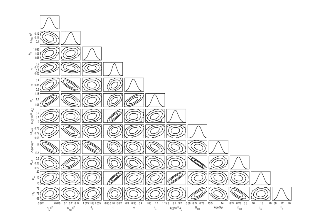
Figure 1: The 1D marginalized distributions on individual parameters and 2D contours with 68%C.L., 95 %C.L., and 99.7%C.L. between each other using the combination of the observational data from WMAP, BAOs and SNIa for the RDE model.

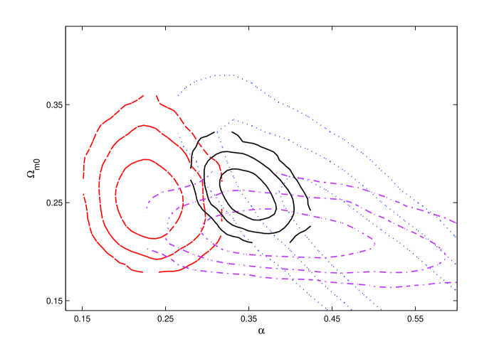
Figure 2: The 2D contours with 68%C.L., 95 %C.L., and 99.7%C.L. between $\alpha$ and $\Omega_{m0}$ for the RDE model from WMAP alone (red dashed line), BAOs alone (magenta dash-dotted line), SNIa alone (blue dotted line), and the combination of WMAP, BAOs and SNIa (solid black line).

In Fig. 3, we show CMB temperature power spectra for the RDE model by using the best-fitting results in Table 1 and for the $\Lambda$CDM model with the best-fit values from the WMAP alone constraint ref:wmap7 and WMAP+BAO+SNIa in Table 1. It is found that there are significant discrepancies of CMB temperature power spectra in the two models on large angular scales, where the contribution to the secondary CMB temperature power spectrum is mainly from the late ISW effect. Both the curves of the CMB temperature power spectra for the RDE model on large angular scales almost tend to be plat. A large-scale ($l<10$) plateau happens in the RDE model. In order to understand the imprint on the CMB temperature power spectrum from parameter $\alpha$ alone, we illustrate the CMB temperature power spectra for different $\alpha$ in Fig. 4. It is shown that the CMB temperature power spectra on all the scales decrease as the value of $\alpha$ becomes smaller. Because $\alpha$ has an effect on the expansion rate, the angular diameter distance to recombination becomes larger when $\alpha$ decreases. So there is the rightward shift of the positions of peaks. What is more, the usual dimensionless densities of the RDE and matter component are changed for different parameters, $\alpha$, as shown in Fig. 5. That is to say, the change in the expansion rate brings about the differences of usual dimensionless densities when there is the same matter density, $\Omega_{m0}$. We can see at early times the usual dimensionless matter density decreases when $\alpha$ become larger. We try to look into the role of the change of $\alpha$ by taking another point of view. We consider that this effect can be viewed as coming from the different effective matter densities based on the same expansion rate, i.e., $\Omega^{eff}_{m0}(1+z)^{3}/E^{2}_{s}$. So there is a lower effective matter density with the increase in $\alpha$. The lower effective matter density causes the delay of the epoch of matter-radiation equality, i.e., the smaller $z_{eq}$. This change in redshift of equality leads to the enhanced late ISW effect on large scales and power spectra on small scales. Furthermore, the delay of the time of dark energy domination for smaller $\alpha$ also leads to the suppressed late ISW effect on large scales. In Fig. 6, we show the evolutions of cold dark matter and dark energy perturbations on the large scale, i.e., $k=0.001\textmd{Mpc}^{-1}$.

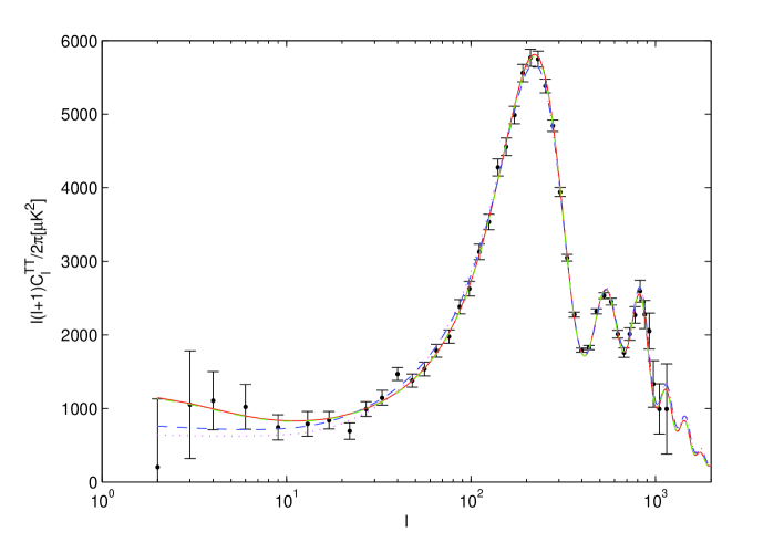
Figure 3: CMB temperature power spectra vs multipole moment $l$, where the black dots with black error bars denote the observed data with their corresponding uncertainties from WMAP, the red solid line is for the $\Lambda$CDM model with the best-fit values from the WMAP alone constraint ref:wmap7 , the green dash-dotted line is for the $\Lambda$CDM model with the best-fit values from the WMAP+BAO+SNIa joint constraint, the blue dashed line is for RDE with the best-fit values from the WMAP alone constraint, and the magenta dotted line is for the RDE model with the best-fit values from the WMAP+BAO+SNIa joint constraint.

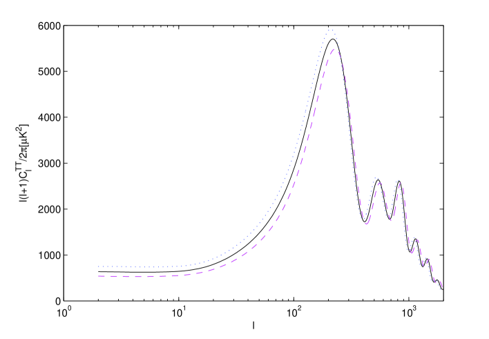
Figure 4: CMB temperature power spectra vs multipole moment $l$ for the RDE model with different parameters, $\alpha$, where the blue dotted line is the power spectrum with $\alpha=0.44$, the black solid line is the power spectrum with the best-fit value of $\alpha$ from the WMAP+BAO+SNIa joint constraint, and the magenta dashed line is the power spectrum with $\alpha=0.24$.

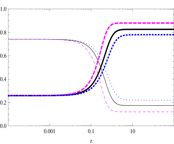
Figure 5: The usual dimensionless energy densities of RDE (thin) $\left(\frac{\Omega_{de}}{E^{2}}\right)$ and matter component (thick) $\left(\frac{\Omega_{m0}(1+z)^{3}}{E^{2}}\right)$ vs redshift $z$ for the RDE model with different parameters, $\alpha$, where the blue dotted lines are dimensionless energy densities with $\alpha=0.44$, the black solid lines are dimensionless energy densities with the best-fit value of $\alpha$ from the WMAP+BAO+SNIa joint constraint, and the magenta dashed lines are dimensionless energy densities with $\alpha=0.24$.

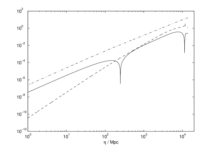
Figure 6: The evolutions of cold dark matter density perturbation, $\delta_{c}$ (dash-dotted line), dark energy density perturbation, $|\delta_{de}|$ (solid line), and its velocity perturbation, $\upsilon_{de}$ (dashed line).

The differences of background evolutions between the $\Lambda$CDM model and RDE model can be seen through the evolutions of the distance moduli and relative distance moduli in Fig. 7. Then following the method of the propagation of errors by the Fisher matrix analysis ref:werror1 ; ref:werror2 ; ref:werror3 , we plot the evolution of EOS with $1\sigma$ errors in Fig. 8 by using the mean values from WMAP+BAO+SNIa. The current value of the EOS is -1.0853, less than -1. What is more, it is seen that the EOS of RDE crosses the cosmological constant boundary at $z\sim 0.05$.

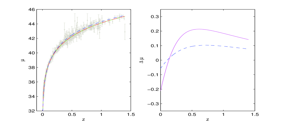
Figure 7: Left panel: The distance moduli $\mu$ vs redshift $z$, where the grey dots with grey error bars denote the observed data with their corresponding uncertainties from SNIa, the red solid line is for the $\Lambda$CDM model with the best-fit values from the WMAP alone constraint ref:wmap7 , the green dash-dotted line is for the $\Lambda$CDM model with the best-fit values from the WMAP+BAO+SNIa joint constraint, the blue dashed line is for the RDE model with the best-fit values from the WMAP alone constraint, and the magenta dotted line is for the RDE model with the best-fit values from the WMAP+BAO+SNIa joint constraint. Right panel: The relative distance moduli $\Delta\mu=\mu_{\textmd{RDE}}-\mu_{\Lambda\textmd{CDM}}$ vs redshift $z$, where the magenta solid line is for the best-fit values from the WMAP alone constraint, and the blue dashed line is for the best-fit values from the WMAP+BAO+SNIa joint constraint.

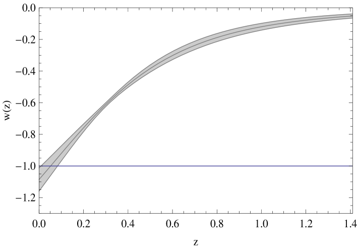
Figure 8: The evolution of the equation of state with $1\sigma$ errors, where the mean values with $1\sigma$ errors for the RDE model from the WMAP+BAO+SNIa joint constraint are used.

IV Summary

In summary, we perform a global fitting on the RDE model with perturbations to the combined constraints from the full CMB data, BAOs, and SNIa by using the MCMC method. All the cosmological parameters for the RDE model are well determined, as shown in Table 1. It is worth noting that the initial power spectrum with a blue tilt is favored for the RDE model. Making use of the constraint results, we investigate the CMB temperature power spectra. It is found that the differences of CMB temperature power spectra on large angular scales are significant between the $\Lambda$CDM model and the RDE model with perturbations. The main feature of CMB temperature power spectra on large angular scales for the RDE model with perturbations is that there exists a flat plateau. In view of the differences of large-scale power spectra, on which the ISW effect plays an important role, the effects on RDE parameters made by the ISW data from the cross correlations of CMB andlarge-scale structure will be worth investigating in future work.

- (1) E. Komatsu et al., Astrophys. J. Suppl. 192, 18 (2011), arXiv:1001.4538.
- (2) M. Tegmark et al., Phys. Rev. D 69, 103501 (2004), astro-ph/0310723.
- (3) M. Tegmark et al., Astrophys. J. 606, 702 (2004), astro-ph/0310725.
- (4) A. Clocchiatti et al., Astrophys. J. 642, 1 (2006).
- (5) R. Amanullah et al., [Supernova Cosmology Project Collaboration], Astrophys. J. 716, 712 (2010), arXiv:1004.1711.
- (6) A. G. Riess et al., Astron. J. 116, 1009 (1998), astro-ph/9805201.
- (7) S. Perlmutter et al., Astrophys. J. 517, 565 (1999), astro-ph/9812133.
- (8) B. Ratra and P. J. E. Peebles, Phys. Rev. D. 37, 3406 (1988); M. S. Turner and M. White, Phys. Rev. D 56, 4439 (1997); R. R. Caldwell, R. Dave, and P. J. Steinhardt, Phys. Rev. Lett. 80, 1582 (1998); P. J. Steinhardt, M. L. Wang, and I. Zlatev, Phys. Rev. D 59, 123504 (1999); R. R. Caldwell, Phys. Lett. B 545, 23 (2002); N. N. Weinberg, Phys. Rev. Lett. 91, 071301 (2003); S. Nojiri and S. D. Odintsov, Phys. Rev. D 72, 023003 (2005); B. Feng, X. L. Wang, and X. M. Zhang, Phys. Lett. B 607, 35 (2005); Z. K. Guo, Y. S. Piao, X. N. Zhang, and Y. Z. Zhang, Phys. Lett. B 608, 177 (2005).
- (9) A. Y. Kamenshchik, U. Moschella, and V. Pasquier, Phys. Lett. B 511, 265 (2001); M. C. Bento, O. Bertolami, and A. A. Sen, Phys. Rev. D 66, 043507 (2002); M. C. Bento, O. Bertolami, M. J. Reboucas, and P. T. Silva, Phys. Rev. D 73, 043504 (2006).
- (10) M. Li, Phys. Lett. B 603, 1 (2004).
- (11) M. Li, X. D. Li, S. Wang, and Y. Wang, arXiv:1103.5870.
- (12) A. G. Cohen, D. B. Kaplan, and A. E. Nelson, Phys. Rev. Lett. 82, 4971 (1999), hep-th/9803132.
- (13) C. Gao, X. Chen, and Y. G. Shen, Phys. Rev. D 79, 043511 (2009), arXiv:0712.1394.
- (14) L. N. Granda and A. Oliveros, Phys. Lett. B 669, 275 (2008), arXiv:0810.3149; Y. T. Wang and L. X. Xu, arXiv:1004.3340.
- (15) L. X. Xu, J. B. Lu, and W. B. Li, Eur. Phys. J. C 64, 89 (2009).
- (16) R.-J. Yang, Z.-H. Zhu, and F. Wu, Int. J. Mod. Phys. A 26, 317 (2011).
- (17) R. G. Cai, B. Hu and Y. Zhang, Commun. Theor. Phys. 51, 954 (2009).
- (18) L. Xu, W. Li, J. Lu, and B. Chang, Mod. Phys. Lett. A 24, 1355 (2009); M. Li, X. Li, and X. Zhang, arXiv:0912.3988; M. Li, X. D. Li, S. Wang, and X. Zhang, JCAP 0906, 036 (2009); L. X. Xu and Y. T. Wang, JCAP 06, 002 (2010).
- (19) X. Zhang, Phys. Rev. D 79, 103509 (2009);
- (20) H. Li, J. Q. Xia, G. B. Zhao, Z. H. Fan, and X. M. Zhang, Astrophys. J. 683, L1-L4 (2008).
- (21) C. G. Park, J. C. Hwang, J. H. Lee, and H. Noh, Phys. Rev. Lett. 103, 151303 (2009).
- (22) R. Bean and O. Dore, Phys. Rev. D 69, 083503 (2004), astro-ph/0307100.
- (23) J. Weller and A. M. Lewis, Mon. Not. Roy. Astron. Soc. 346, 987 (2003).
- (24) G. B. Zhao, J. Q. Xia, M. Li, B. Feng, and Xinmin Zhang, Phys. Rev. D 72, 123515 (2005), astro-ph/0507482.
- (25) J. Q. Xia, G. B. Zhao, B. Feng, H. Li, and Xinmin Zhang, Phys. Rev. D 73, 063521 (2006), astro-ph/0511625.
- (26) G. B. Zhao, J. Q. Xia, B. Feng, and Xinmin Zhang, Int. J. Mod. Phys. D 16, 1229 (2007), astro-ph/0603621.
- (27) J. Q. Xia, Y. F. Cai, T. T. Qiu, G. B. Zhao, and Xinmin Zhang, Int. J. Mod. Phys. D 17, 1229 (2008), astro-ph/0703202.
- (28) J. Q. Xia, H. Li, G. B. Zhao, and Xinmin Zhang, Phys. Rev. D 78, 083524 (2008), arXiv:0807.3878;
- (29) R. K. Sachs and A. M. Wolfe, Astrophys. J. 147, 73 (1967).
- (30) B. M. Schaefer, Mon. Not. Roy. Astron. Soc. 388, 1403 (2008), arXiv:0803.2239.
- (31) Y. T. Wang, Y. X. Gui, L. X. Xu, and J. B. Lu, Phys. Rev. D 81, 083514 (2010).
- (32) G. Olivares, F. A. Brandela, and D. Pavon, Phys. Rev. D 77, 103520 (2008).
- (33) J. B. Dent, S. Dutta, and T. J. Weiler, Phys. Rev. D 79, 023502 (2009).
- (34) D. Sapone and M. Kunz, Phys. Rev. D 80, 083519 (2009).
- (35) Y. T. Wang, L. X. Xu, and Y. X. Gui, Phys. Rev. D 82, 083522 (2010).
- (36) J. M. Bardeen, Phys. Rev. D 22, 1882 (1980).
- (37) H. Kodama, and M. Sasaki, Prog. Theo. Phys. Supp. 78, 1 (1984).
- (38) C. P. Ma and E. Bertschinger, Astrophys. J. 455, 7 (1995).
- (39) W. Hu and D. J. Eisenstein, Phys. Rev. D 59, 083509 (1999).
- (40) K. A. Malik and D. Wands, Phys. Rept. 475, 1 (2009).
- (41) http://cosmologist.info/cosmomc/.
- (42) A. Lewis and S. Bridle, Phys. Rev. D 66, 103511 (2002).
- (43) http://camb.info/.
- (44) Ch. Yeche, A. Ealet, A. Refregier, C. Tao, A. Tilquin, J.-M. Virey, and D. Yvon, astro-ph/0507170; P. S. Corasaniti, M. Kunz, D. Parkinson, E. J. Copeland, and B. A. Bassett, Phys. Rev. D 70, 083006 (2004).
- (45) S. Burles, K. M. Nollett, and M. S. Turner, Astrophys. J. 552, L1 (2001).
- (46) A. G. Riess et al., Astrophys. J. 699, 539 (2009), arXiv:0905.0695.
- (47) http://lambda.gsfc.nasa.gov/product/map/current/.
- (48) W. J. Percival et al., Mon. Not. Roy. Astron. Soc. 401, 2148 (2010), arXiv:0907.1660.
- (49) W. H. Press et al., Numerical Recipes, Cambridge University Press (1994).
- (50) U. Alam, V. Sahni, T. D. Saini, and A. A. Starobinsky, astro-ph/0406672.
- (51) S. Nesseris and L. Perivolaropoulos, Phys. Rev. D 72, 123519 (2005), astro-ph/0511040.
- (52) T. D. Kitching and A. Amara, arXiv:0905.3383.