Kolmogorov scaling bridges linear hydrodynamic stability and turbulence

Abstract

The way in which kinetic energy is distributed over the multiplicity of inertial (intermediate) scales is a fundamental feature of turbulence. According to Kolmogorov’s 1941 theory, on the basis of a dimensional analysis, the form of the energy spectrum function in this range is the $-5/3$ spectrum. Experimental evidence has accumulated to support this law. Until now, this law has been considered a distinctive part of the nonlinear interaction specific to the turbulence dynamics. We show here that this picture is also present in the linear dynamics of three-dimensional stable perturbation waves in the intermediate wavenumber range. Through extensive computation of the transient life of these waves, in typical shear flows, we can observe that the residual energy they have when they leave the transient phase and enter into the final exponential decay shows a spectrum that is very close to the $-5/3$ spectrum. The observation times also show a similar scaling. The scaling depends on the wavenumber only, i.e. it is not sensitive to the inclination of the waves to the basic flow, the shape-symmetry of the initial condition and the Reynolds number.

In fluid systems, stability and turbulence are the two faces of the same coin. The existence of equilibrium: in one case laminar, and steady in the mean in the other. The link between these two faces is transition D2002 ; CJJ2003 ; SH2001 ; K41 ; F95 ; SA97 .

Unfortunately, or fortunately, depending on the circumstances, turbulence is the rule and not the exception in fluid motion. When the energy forcing in the system is sufficiently high, transition to turbulence occurs in the short or in the long term. In principle, stability and turbulence studies are intimately connected. In practice, the relevant literature is split into two quite distinct fields (however, counterexamples exist, see e.g. Hof2004 ; Hof2006 ). The main reason is that the stability can be defined physically as the ability of a dynamical system to be immune to small disturbances, which necessarily leads to the linearization of the mathematical formulation. This is something which cannot occur in turbulence where a great number of several interacting scales are always active and experimentally observable.

However, at any instant, laminar systems host a multiplicity of scales: the small perturbations which randomly enter the system and, in the linear framework, evolve independently from each other. Although linearity on one hand allows each evolution to be determined singularly, on the other, it should be recalled that a large number of perturbations (not even bounded, in principle) are present at the same time. In this work, we have tried to consider and observe the collective behavior of small perturbations, in particular, those filling the intermediate range of wave lengths that the system can host. The aim is the understanding and discovering of possible similarities with turbulence behavior.

As an example, in order to understand whether, and to what extent, spectral representation can effectively highlight the nonlinear interaction that occurs among different scales, it could be useful to consider the state that precedes the onset of both instability and turbulence in flows. In this condition, even if stable, the system is however subject to a swarming of small arbitrary three-dimensional perturbations that constitutes a system of multiple spatial and temporal scales subject to all the processes included in the Navier-Stokes equations: linearized convective transport, linearized vortical stretching and tilting, and molecular diffusion. If we leave nonlinear interaction of the different scales, the other features are tantamount to the features of the turbulent state.

If it were possible to observe such a system, by computing and comparing a large set of three dimensional waves, and build spectra, it would be possible, among others, to determine if a power scaling in the intermediate range exists and, in case, to compare it with the exponent of the corresponding developed turbulent state (notoriously equal to - 5/3). In the case a power scaling exists, two possible situations can therefore appear. A - The exponent difference is large, and as such, is a quantitative measure of the nonlinear interaction in spectral terms. B - The difference is small. This would indicate a higher level of universality on the value of the exponent of the intermediate range (the inertial range in turbulence), not necessarily associated to the nonlinear interaction.

For this purpose, by solving a large number of initial-value problems, we have determined a large set of transient solutions (a database of 2400 solutions, see the Supplemental Material, section 5) for two typical shear flows: a plane channel flow, archetype of wall flows, and a two-dimensional bluff-body wake, archetype of free-flows, see Fig. 1 a. Perturbations that randomly arrive in the system undergo a transient evolution which is ruled by the initial-value problem associated to the Navier-Stokes linearized formulation K1880 ; O1907a ; O1907b . These problems must be parameterized through the principal physical and geometrical quantities that can influence the life of perturbation waves, the angle of obliquity, the symmetry, the polar wavenumber and Reynolds number. For instance, the wavelength of the waves can be varied in a range as large as the range of scales that typically fill the field when the system is in the so-called fully developed turbulent state.

There exists many kinds of transient behavior, very different and not all of which is trivial (for a description, see the text below and in particular the overview presented in figure 2). The transient lives can last a few basic time scales (external length referred to the velocity scale of the basic flow) as well as order $10^{4}$ time scales. During these lives energy can be accumulated, then smoothly lost or lost and acquired again. Usually, different inner time scales appear. For instance, the pulsation can change in a discontinuous way before the asymptotic state is reached. This very rich scenario is met out of any self-interaction and interaction with other waves and, to some degree, is reminiscent, at least qualitatively, of the turbulence phenomenology.

So, the question arises: how to compare spectrally the set of very different transients of large, intermediate and short waves? Our answer is that whatever be the difference in the wave lives, a common phase exits: the time interval where the wave exits the transient and enters the exponential asymptotic state. We thus consider the residual kinetic energy owned by the waves in this interval and build a spectrum in the wavenumber space.

Let us now describe synthetically the basic flows we have here analyzed, as well as the relevant transient computation. The basic flows for a channel flow are represented by the Poiseuille solution (see Fig. 1b and SM, section 4), and for a wake by the first two order terms of the Navier-Stokes asymptotic solution described in TB03 (see Fig. 1c and SM, section 4). The channel flow is homogeneous along the streamwise and spanwise directions ($x$ and $z$). The profiles only vary with the coordinate $y$. In the case of the wake, the profiles also slowly evolve with $x$. As a consequence, the flow is not perfectly parallel and we consider two fixed longitudinal stations in the region of the wake where entrainment is present TS09 , $x_{0}=10,50$ ($x_{0}$ is the distance from the body normalized over the body length). Different Reynolds numbers (the dimensionless control parameter that gives the order of magnitude of the ratio between convection and molecular diffusion) are considered for each example of flow: subcritical (steady laminar solution: $Re=30$ for the wake, $Re=500$ for the channel), supercritical (unstable laminar wake $Re=50,100$ and turbulent channel $Re=10000$). An initial-value problem (IVP) for small arbitrary three-dimensional vorticity perturbations imposed on the basic shear flows is then considered. The viscous perturbation equations are combined in terms of the vorticity and velocity CD90 , and are solved by means of a combined Fourier–Fourier (channel) and Laplace–Fourier (wake) transform in the plane normal to the basic flow, see SM section 4 and CJJ2003 ; STC09 ; STC10 . The exploration is conducted with respect to physical quantities, such as the polar wavenumber, the angle of obliquity, the symmetry of the perturbation, the flow control parameter, and, for the wake, which is not parallel, the position downstream of the body. For further details on the formulation and the numerical methods used to solve the initial-value problems see the Supplemental Material (SM, section 4).

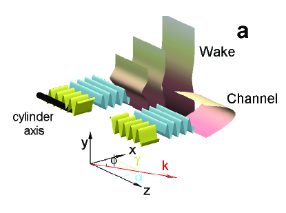
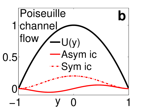
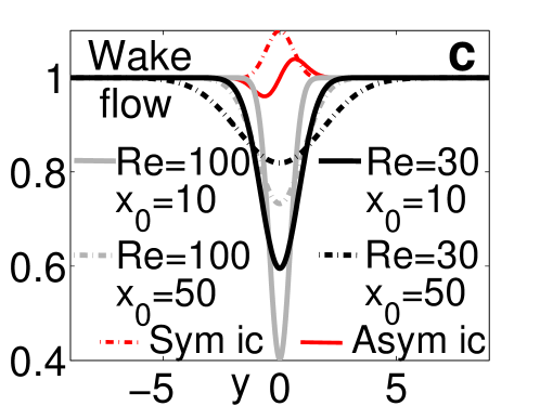
Figure 1: (a) Base flows and perturbation scheme. The flow profiles are qualitatively represented in pink. The perturbation is represented by the blue and the yellow waves which propagate in the $x$ and $z$ directions, respectively. $k=\alpha\textbf{i}+\gamma\textbf{k}$ is the wavenumber, $\phi$ is its inclination angle with respect to the basic flow. (b)-(c) Initial conditions and velocity profiles. The red dotted and solid lines are the symmetric and asymmetric parts of the initial perturbations, respectively. The grey and black lines in the wake panel (c) schematically show the velocity variation with the Reynolds number ($Re$) and the position in the wake, $x_{0}$. Grey lines: supercritical $Re$ (the critical value is $47$), black lines: subcritical value. Dotted lines: far wake field, solid lines: intermediate field.

To measure the temporal evolution of the energy of each perturbation, we define the kinetic energy density, $\displaystyle{e(t;\alpha,\gamma)=\frac{1}{2}\int_{-y_{f}}^{+y_{f}}(|\hat{u}|^{2}+|\hat{v}|^{2}+|\hat{w}|^{2})dy}$, where $-y_{f}$ and $y_{f}$ are the computational limits of the domain, $\hat{u}$, $\hat{v}$ and $\hat{w}$ are the transformed velocity components of the perturbation. We can also define the amplification factor, $G$, as the kinetic energy density normalized with respect to its initial value, $G(t;\alpha,\gamma)=e(t;\alpha,\gamma)/e(t=0;\alpha,\gamma)$.

In terms of amplification factors, the early transient evolution offers very different scenarios for which we present in the following a summary of relevant cases. For example, for both base flows, we have observed that the orthogonal waves are always asymptotically stable. However, the perturbations are able to reach very high maxima of the amplification factor $G$ (of the order of $10^{4}$, see Fig. 2b) before the transients are extinguished. Non-orthogonal asymmetric waves present as well transients which are not trivial at all (see blue and red solid lines in Fig. 2a and 2c). These perturbations are slightly amplified in the early stage of their lives, then decrease for several hundreds of time scales and in the end they grow with the same slope of the correspondent symmetric waves (compare the asymptotic trends of non-orthogonal solid and dotted curves in panels a and c of Fig. 2). During the decreasing phase, these transients clearly show an initial oscillatory time scale associated to a modulation in amplitude of the average value of the pulsation in the early transient, and which is different from the asymptotic value of the pulsation (see the insets in panels a-c in Fig. 2)STC09 . Here the pulsation (angular frequency), $\omega$, is defined as the time derivative of the wave phase at a fixed transversal position (see SM, section 4). Thus, the system exhibits two distinct temporal oscillatory patterns, the first, of transient nature, and, the second one, of asymptotic nature.

As a general comment, the most important parameters affecting these configurations are the angle of obliquity, the symmetry, and the polar wavenumber. While the symmetry of the disturbance influences the transient behavior to a great extent and leaves the asymptotic fate unaltered, a variation in the obliquity and in polar wavenumber can significantly change the early trend as well as the final stability configuration.

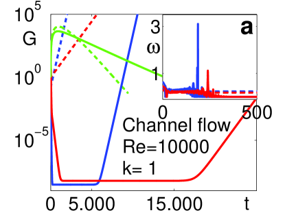
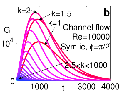
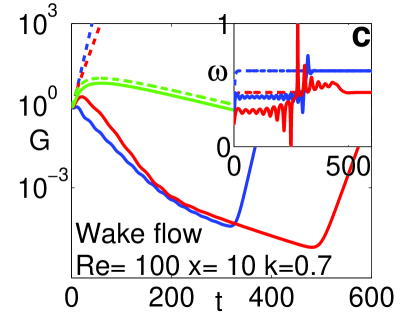
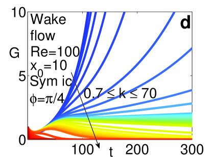
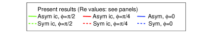
Figure 2: Collection of transient lives of the perturbations observed through the amplification factor $G$. Left column: the magnitude of the wavenumber is fixed, while the obliquity and symmetry vary (see the legend on the bottom). The insets (temporal evolution of the pulsation, $\omega$) highlight the typical formation of time scales others than the flow external time scale and the wave period. Right column: transients variation with changes in the wavenumber magnitude.

The asymptotic behavior for the plane wake, for disturbances aligned to the flow, is shown to be in excellent agreement ETC12 with 2D spatio-temporal modal analyses TSB06 ; BT06 and with the laboratory determined frequency and wave length of the parallel vortex shedding at $Re=50$ and $100$ W89 . See also in the SM, the section Asymptotic pulsation (section 3, figure S3) where information on the channel flow pulsation measured in the laboratory and from the present IVP computations are given.

We now come back to the spectral analysis of common phase in the lives of the perturbations, that is the transition between the end of the transients and the settlement of the asymptotic condition. To compare the residual kinetic energy of the waves in correspondence to this transition, we assumed that when the asymptotic exponential temporal behavior is reached, the temporal growth rate, $r$, defined as $r(t;\alpha,\gamma)=log(e)/(2t)$ CJJ2003 , must approach a real constant.

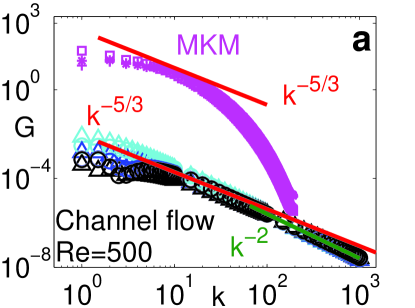
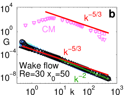
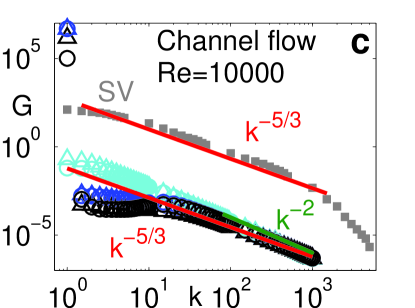
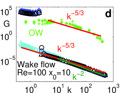
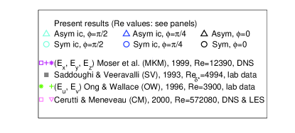
Figure 3: Spectra of the amplification factor G for the collections of linear traveling waves observed at the time, $T_{e}$, where the perturbations are out of their transient. The spectra obtained in this study have been compared qualitatively with the turbulent field spectra available in the literature and obtained from laboratory or numerical experiments. The legend in the bottom panel specifies the symbols associated with either the results of the present study or those of the laboratory, and numerical experiments carried out on fully turbulent flow fields by other authors.

In order to determine the temporal region in which the evolution behaves exponentially, it is necessary to monitor the instants beyond which the condition $r\rightarrow const$ is satisfied. Doing this, we introduce a necessary condition, that, however, is not sufficient to determine the instants where the perturbations can be compared. In fact, the transition toward the exponential behavior is smooth, very long, and different from case to case (in some instances, it can be oscillatory). As a result, it is not numerically efficient to obtain the instants where $r$ starts to be constant. We have thus associated a second condition to be satisfied together with the constancy of the growth rate, which directly acts on the energy temporal rate of variation. To this aim, we have selected the instants at which the amplification factor reaches a given rate of variation, either in growth or in decay. This situation is represented by the instant, that we call observation time, $T_{e}$, where $dG/dt<\epsilon$ or $dG/dt>1/\epsilon$, with $\epsilon=10^{-n}$. Here, $n$ is an arbitrary positive quantity (for instance, a positive integer) that we have fixed equal to 4. It is possible to show that the present results – in particular, the existence of an intermediate spectral range where the spectral decay exponent is very close to that of the Kolmogorov theory – do not depend on the choice of $n$ (see SM, section 1).

In Fig. 3 and 4, the results of the measure of the energy residuals out of the transients are shown. The spectral values of $G$, for both the channel flow case (panels a,c) and the wake flow case (panels b,d) show a scaling in the intermediate range of the polar wavenumber ($k\in[10,200]$ for the channel, $k\in[2,50]$ for the wake) that is amazingly close to the turbulent canonical value of $-5/3$. For shorter wavelengths, characterized by very short transients, the scaling is a little higher in magnitude, approximatively equal to $-2$. This result does not appear to be influenced to any great extent by the wave obliquity, the symmetry, or the $Re$. However, it is possible to observe that purely orthogonal waves show a closer scaling to $-2$ than to $-5/3$, even at intermediate wavenumbers. In general, a full decade of intermediate wavenumbers can be observed for both the wall flow and the free flow. These data gather all the stable waves occurring in the intermediate range and in the dissipative range. We would like to point out that the data do not highlight a dependence on $Re$, the flow control parameter. For longer waves ($k<10$ and $k<1-2$ for the plane Poiseuille flow and the bluff-body wake, respectively), the results depend on the perturbation inclination, the symmetry of the initial condition, and on the boundary conditions (geometry of the system). As expected, they do not reveal any universal behavior. In Fig. 3, panels a-b-c-d, experimental (laboratory and numerical) measurements MKM1999 ; SV1993 ; CM2000 ; OW1996 in the turbulent states have been included for the sake of comparison of stable linear perturbations and turbulent scales.

These results appear strengthened by the fact that even the observation times, $T_{e}$, present the same scaling, see Fig. 4. This outcome is not at all trivial. It is sufficient to consider that the observation time includes the transient, and that the different kind of transients we observed are very complex and can vary in length over 4 orders of magnitude when moving across the space of parameters (the wavenumber, the symmetry, the obliquity, the flow control parameter, Re, and, in the case of a basic evolving spatial flow, the position).

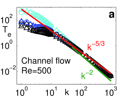
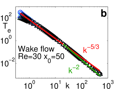
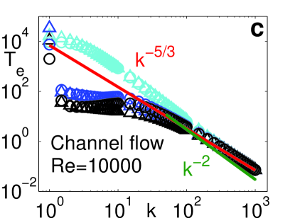
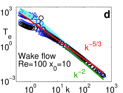
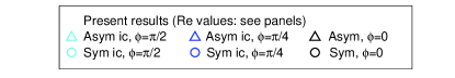
Figure 4: Spectrum of the observation time where the wave energy is measured and compared. The data refer to the entire collection of linear perturbations shown in figure 3. Stable basic flows (top panels), unstable flows (bottom panels). The plane channel flow is on the left, the bluff body wake is on the right. Symmetric (circles) and asymmetric (triangles) initial perturbations. Obliquity angles: $\phi=0$ (black), $\phi=\pi/4$ (blue) and $\phi=\pi/2$ (cyan). It is possible to observe an abundant decade where longitudinal, oblique and orthogonal perturbations present a power-law decay which is close to -5/3 (red curves). Larger wavenumbers, which are influenced more by diffusion-dissipative processes, steep towards a decay exponent of about -2.

A possible scenario for fields with a sufficiently high Reynolds number to be in a turbulent state, which includes the present findings, could be the following. The nonlinear interaction works intensively on the long waves that are unstable by blocking the linear growth and by settling their kinetic energy to a level that can be associated with the global Reynolds number of the system. The surplus of energy that the unstable waves potentially gain during the linear evolution is then transferred to shorter waves, that are longitudinal, oblique or orthogonal to the basic velocity field. The transfer is particularly intense for asymptotically stable intermediate waves (namely the inertial scales, according to the terminology used in turbulence). It is possible to suppose that the transfer is physically triggered during the phases where the amplification factor is maximum, see Figure 2. This process continues and the energy in the range of intermediate waves reaches values that can be experimentally observed, in the laboratory, or in the so called Navier-Stokes direct numerical solutions. Taking into account the present results, it is possible to say that the nonlinear interaction distributes the relative energy over different wavenumbers in a way that corresponds to the relative residual energy each wave has when, after the transient, it reaches a common decay threshold. This process is less efficient on short waves. For these waves, the maximum of the amplification factor becomes progressively smaller as the wavenumber magnitude increases (see Figure 2b) and, as a consequence, it is more difficult for them to couple with longer waves. A rapid fall in energy to levels many orders of magnitude lower, and, thus closer to the specific levels of their linear evolution, is therefore observed in the experimental spectra (see Figure 3).

In conclusion, we have observed a fingerprint of the Kolmogorov scaling inside the collective behavior of transient intermediate perturbation waves, which always are asymptotically stable. These new observations are not specific of a peculiar kind of flow (wall bounded or free). This can mean that this scaling is not only one of the major signatures of the turbulence interaction, but it also exists hidden inside the dynamics of linear stable waves, where even the self-interaction is absent. Since our observations do not depend on the system control parameter (Reynolds number), on the kind of initial condition and on geometrical parameters, such as the wave inclination, they could also reveal a new set of structural properties of the Navier-Stokes equation solutions. In particular, we think that they can be used to build a bridge between the linear and the nonlinear interaction in multi-scale systems. Given the high variability of the shape and length of the transient life, we consider remarkable that the Kolmogorov scaling does not appear only in the energy spectra, but also in the spectra of the observation times.

For the critical and useful exchanges had during her visit, D.T. acknowledges the 2011 program The Nature of Turbulence, held at the Kavli Institute for Theoretical Physics of the University of California Santa Barbara. For helpful comments D.T. acknowledges Katepalli R. Sreenivasan, and, together with S.S., William O. Criminale and B. Eckhardt. The authors thank Marco Mastinu for his contribution to the numerical simulations. This study is in part supported by the Progetto Lagrange Foundation.

References

- (1) P. G. Drazin, Introduction to hydrodynamic stability (Cambridge University Press, 2002).
- (2) W. O. Criminale, T. L. Jackson, R. D. Joslin, Theory and Computation in Hydrodynamic Stability (Cambridge University Press, 2003).
- (3) P. J. Schmid, D. S. Henningson, Stability and Transition in Shear Flows (Springer, 2001).
- (4) A. N. Kolmogorov, Dokl. Akad. Nauk SSSR 30, 299-303 (1941).
- (5) U. Frisch, Turbulence: The Legacy of A. N. Kolmogorov (Cambridge University Press, 1995).
- (6) K. R. Sreenivasan, R. A. Antonia, Annu. Rev. Fluid Mech. 29, 35-72 (1997).
- (7) B. Hof, C. W. H. van Doorne, J. Westerweel, F. T. M. Nieuwstadt, H. Faisst, B. Eckhardt, H. Wedin, R. R. Kerswell, F. Waleffe, Science 305, 1594-1598 (2004).
- (8) B. Hof, J. Westerweel, T. M. Schneider, B. Eckhardt, Nature 445, 59-62 (2006).
- (9) Lord Kelvin, Nature 23, 45-46 (1880).
- (10) W. M’F. Orr, Proc. R. Irish. Acad. 27, 9-68 (1907).
- (11) W. M’F. Orr, Proc. R. Irish. Acad. 27, 69-138 (1907).
- (12) D. Tordella, M. Belan, Phys. Fluids 15, 1897-1906 (2003).
- (13) D. Tordella, S. Scarsoglio, Phys. Lett. A 373, 1159-1164 (2009).
- (14) W. O. Criminale, P. G. Drazin, Stud. Applied Math. 83, 123-157 (1990).
- (15) S. Scarsoglio, D. Tordella, W. O. Criminale, Stud. Applied Math. 123, 153-173 (2009).
- (16) S. Scarsoglio, D. Tordella, W. O. Criminale, Phys. Rev. E 81, 036326 (2010).
- (17) S. Scarsoglio, D. Tordella, W. O. Criminale, Springer Proceedings in Physics - Advances in Turbulence XII 132, 155-158 (2009).
- (18) D. Tordella, S. Scarsoglio, M. Belan, Phys. Fluids 18, 054105 (2006).
- (19) M. Belan, D. Tordella, J. Fluid Mech. 552, 127-136 (2006).
- (20) C. H. K. Williamson, J. Fluid Mech. 206, 579-627 (1989).
- (21) R. D. Moser, J. Kim, N. N. Mansour, Phys. Fluids 11, 943-945 (1999).
- (22) S. G. Saddoughi, S. V. Veeravalli, J. Fluid Mech. 268, 333-372 (1994).
- (23) S. Cerutti, C. Meneveau, Phys. Fluids 12, 1143-1165 (2000).
- (24) L. Ong, J. Wallace, Exp. Fluids 20, 441-453 (1996).