Timelike Constant Mean Curvature Surfaces with Singularities

Abstract.

We use integrable systems techniques to study the singularities of timelike non-minimal constant mean curvature (CMC) surfaces in the Lorentz-Minkowski 3-space. The singularities arise at the boundary of the Birkhoff big cell of the loop group involved. We examine the behaviour of the surfaces at the big cell boundary, generalize the definition of CMC surfaces to include those with finite, generic singularities, and show how to construct surfaces with prescribed singularities by solving a singular geometric Cauchy problem. The solution shows that the generic singularities of the generalized surfaces are cuspidal edges, swallowtails and cuspidal cross caps.

1. Introduction

The study of singularities of timelike constant mean curvature (CMC) surfaces in Lorentz-Minkowski $3$-space $\mathbb{L}^{3}$, initiated in this article, has two contexts in current research: One context is the use of loop group techniques in geometry, whereby special submanifolds are constructed from, or represented by, simple data via loop group decompositions. When the underlying Lie group is non-compact the decomposition used in the construction breaks down on certain lower dimensional subvarieties. It is of interest to understand what effect this has on the special submanifold.

The second context is the study of surfaces with singularities. This has gained some attention in recent years: see, for example [9, 10, 11, 13, 14, 16, 18, 19] and related works. Singularities arise naturally and frequently in geometry: one motivation for their study is that many surface classes have either no, or essentially no, complete regular examples, the most famous case being pseudospherical surfaces. One generalizes the definition of a surface to that of a frontal, a map which is immersed on an open dense subset of the domain and has a well defined unit normal everywhere. A basic question is to find the generic singularities for a given surface class. For example, the generic singularities of constant Gauss curvature surfaces in Euclidean $3$-space are cuspidal edges and swallowtails [12], whilst spacelike mean curvature zero surfaces in $\mathbb{L}^{3}$ have cuspidal cross caps in addition to the two singularities just mentioned [20]. The point is that different geometries have different generic singularities. The first-named of the present authors studied singularities of spacelike non-zero CMC surfaces in $\mathbb{L}^{3}$ in [2], of which more below, but the singularities of timelike CMC surfaces appear to be uninvestigated.

In the loop group context, solutions are generally obtained via either the Iwasawa decomposition $\Lambda G^{\mathbb{C}}=\Omega G\,\cdot\,\Lambda^{+}G^{\mathbb{C}}$, a situation which includes harmonic maps into symmetric spaces, or via the Birkhoff decomposition $\Lambda G=\Lambda^{-}G\cdot\Lambda^{+}G$, a situation which includes Lorentzian harmonic maps into Riemannian symmetric spaces. Both of these types of harmonic maps correspond to various well-known surfaces classes, such as constant Gauss or mean curvature surfaces in space forms – for surveys of some of these, see [1, 8]. When the real form $G$ is non-compact, the left hand side of the decomposition is replaced by an open dense subset, the big cell, of the loop group, rather than the whole. Since, at the global level, there is no general way to avoid the big cell boundary, there remains the question of what happens to the surface at this boundary.

The Riemannian-harmonic (Iwasawa) case was investigated in [2, 4], through the study of spacelike CMC surfaces in $\mathbb{L}^{3}$. The big cell boundary is a disjoint union $\mathcal{P}_{\pm 1}\cup\mathcal{P}_{\pm 2}\cup....$ of smaller cells, with increasing codimension. The lowest codimension small cells, $\mathcal{P}_{\pm 1}$, where generic singularities would occur, were analyzed, and it was found that finite singularities occur on one of these, whilst the surface blows up at the other. In [2] a singular Björling construction was devised to construct prescribed singularities, and the generic singularities for the generalized surface class defined there were found to be cuspidal edges, swallowtails and cuspidal cross caps.

In the present work, we turn to the Lorentzian-harmonic (Birkhoff) situation, and study the example of timelike CMC surfaces. The loop group construction differs from the spacelike case in that the basic data are now two functions of one variable, rather than the one holomorphic function of the Riemannian harmonic case. The Birkhoff decomposition construction compared to the Iwasawa construction, as well as the hyperbolic as opposed to elliptic nature of the problem, pose new challenges. However, we obtain analogous results to those of the spacelike case in [2] and [4].

1.1. Results of this article

The generalized d’Alembert representation used here, which was given by Dorfmeister, Inoguchi and Toda [6], allows one to construct all timelike CMC surfaces from pairs of functions of one variable $\hat{X}(x)$ and $\hat{Y}(y)$ which take values in a certain real form of the loop group $\Lambda G^{\mathbb{C}}$, where $G=\mathrm{SL}(2,{\mathbb{R}})$. The construction depends crucially on a pointwise Birkhoff decomposition of the map $\hat{\Phi}(x,y):=\hat{X}^{-1}(x)\hat{Y}(y)$. The data are thus at the big cell boundary at $z_{0}=(x_{0},y_{0})$ if $\hat{\Phi}(z_{0})$ is not in the Birkhoff big cell. The complement of the big cell is a disjoint union $\bigcup_{j=1}^{\infty}\mathcal{P}_{L}^{\pm j}$ of subvarieties. The codimension of the small cells increases with $|j|$, and therefore generic singularities should occur only on $\mathcal{P}_{L}^{\pm 1}$. We prove in Theorem 5.2 that if $\hat{\Phi}(z_{0})\in\mathcal{P}_{L}^{1}$ then the surface has a finite singularity, and at $\mathcal{P}_{L}^{-1}$ the surface blows up. To investigate the type of the finite singularity, we define generalized timelike CMC surfaces to be surfaces that can locally be represented by d’Alembert data which maps into the union of the the big cell and $\mathcal{P}_{L}^{1}$.

We restrict the discussion to singularities that are semi-regular, that is, where the differential of the surface $f$ has rank $1$, a condition that can be prescribed in the data $\hat{X}$ and $\hat{Y}$. These surfaces are frontals, and there is a well defined (up to local choice of orientation) Euclidean unit normal ${\bf n}_{E}$, which can be locally expressed by $f_{x}\times f_{y}=\chi{\bf n}_{E}$. The function $\chi$ obviously vanishes at points where $f$ is not immersed, and we generally study non-degenerate singularities, that is, points where $\textup{d}\chi\neq 0$.

On generalized timelike CMC surfaces, one finds that singularities come in two classes, which we call class I and class II, respectively characterized geometrically by the property that the direction ${\bf n}_{E}$ is not or is lightlike in $\mathbb{L}^{3}$. Class I singularities never occur at the big cell boundary, but rather due to one of the maps $\hat{X}$ or $\hat{Y}$ not satisfying the regularity condition for a smooth surface. We discuss these singularities in Section 4 and prove that the generic singularities are cuspidal edges. Such singularities can easily be prescribed by choosing $\hat{X}$ and $\hat{Y}$ accordingly, but there is no unique solution for the Cauchy problem for such a singular curve, because it is always a characteristic curve for the underlying PDE.

Class II singularities, on the other hand, always occur at the big cell boundary, and are the real object of interest in this article. Note that, although in this case the tangent to the singular curve is lightlike, this does not mean that the curve is characteristic in the coordinate domain, in contrast to the situation on an immersed surface. The curve can be either non-characteristic or characteristic, and generic non-degenerate singularities, studied in Section 6, are non-characteristic. In Section 6.1, we prove that all generalized timelike CMC surfaces with non-characteristic class II singular curves can be produced by certain "singular potentials".

In Section 6.3, Theorem 6.7, we find the singular potentials which solve the non-characteristic singular geometric Cauchy problem, (Problem 6.6), which is to find the generalized timelike CMC surface with prescribed non-characteristic singular curve, and an additional (geometrically relevant) vector field prescribed along the curve. The non-singular version of this problem was solved in [5], using the generalized d’Alembert setup. It is not possible to apply the non-singular solution to the singular case because the solution depends on the construction of an $\mathrm{SL}(2,{\mathbb{R}})$ frame for the surface, along the curve, directly from the geometric Cauchy data. However, the $\mathrm{SL}(2,{\mathbb{R}})$ frame blows up and is not defined at the big cell boundary, necessitating a work-around.

The solution of the singular geometric Cauchy problem is critical to the study of generic singularities in Section 6.4. The geometric Cauchy data consists of three functions $s(v)$, $t(v)$ and $\theta(v)$ along a curve, which are more or less arbitrary. The singularity at the point $v=0$ is non-degenerate if and only if $\theta^{\prime}(0)\neq 0$ and $s(0)\neq\pm t(0)$. Given this assumption, the main result of this section, Theorem 6.8, states that we have the following correspondences:

cuspidal edge $$\leftrightarrow s(0)\neq 0\neq t(0),$$

swallowtail $$\leftrightarrow s(0)=0,\textup{ and }s^{\prime}(0)\neq 0,$$

cuspidal cross cap $$\leftrightarrow t(0)=0,\textup{ and }t^{\prime}(0)\neq 0.$$

This shows that the generic non-degenerate singularities are just these three, since the only other possibility is a higher order zero.

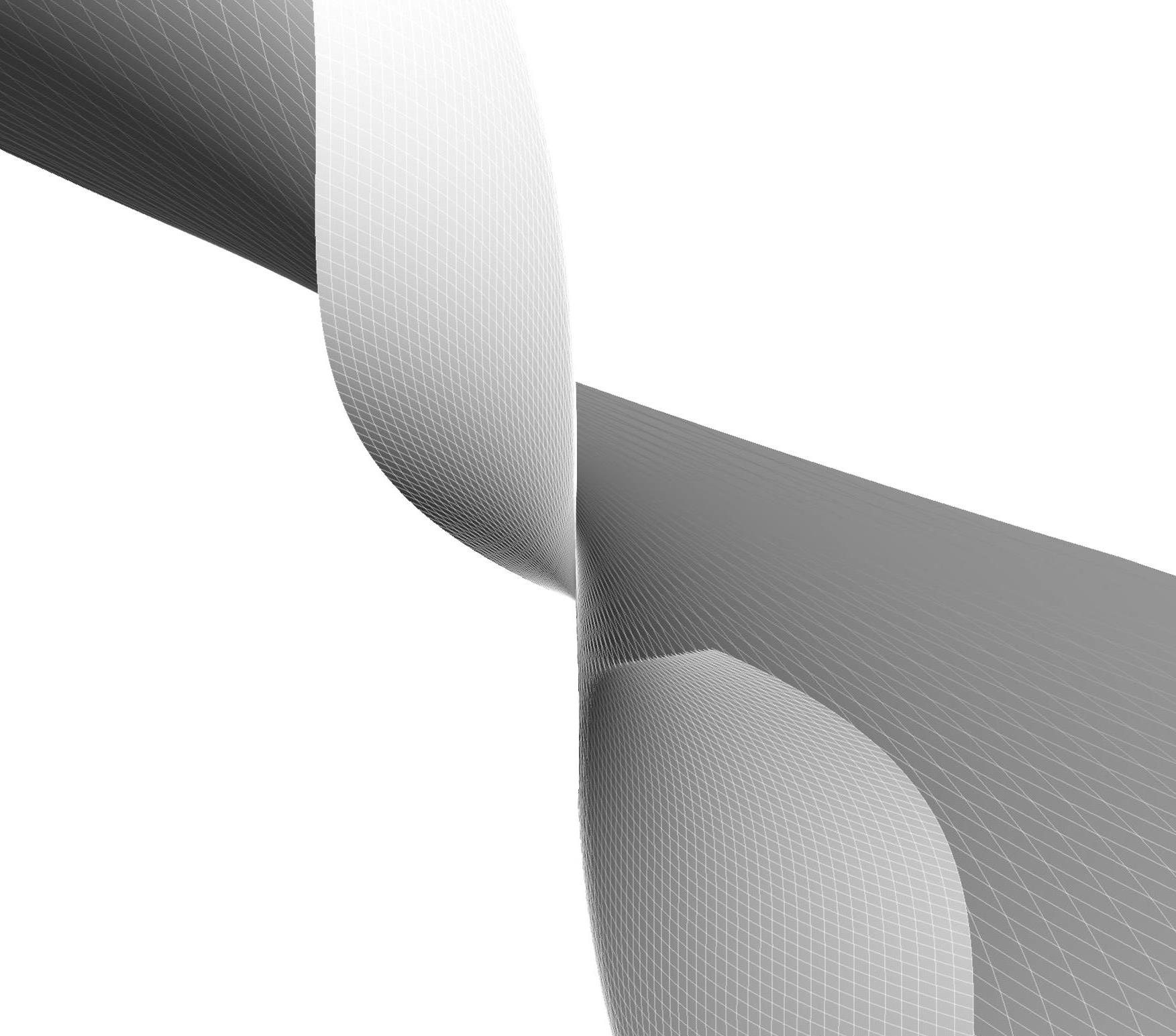
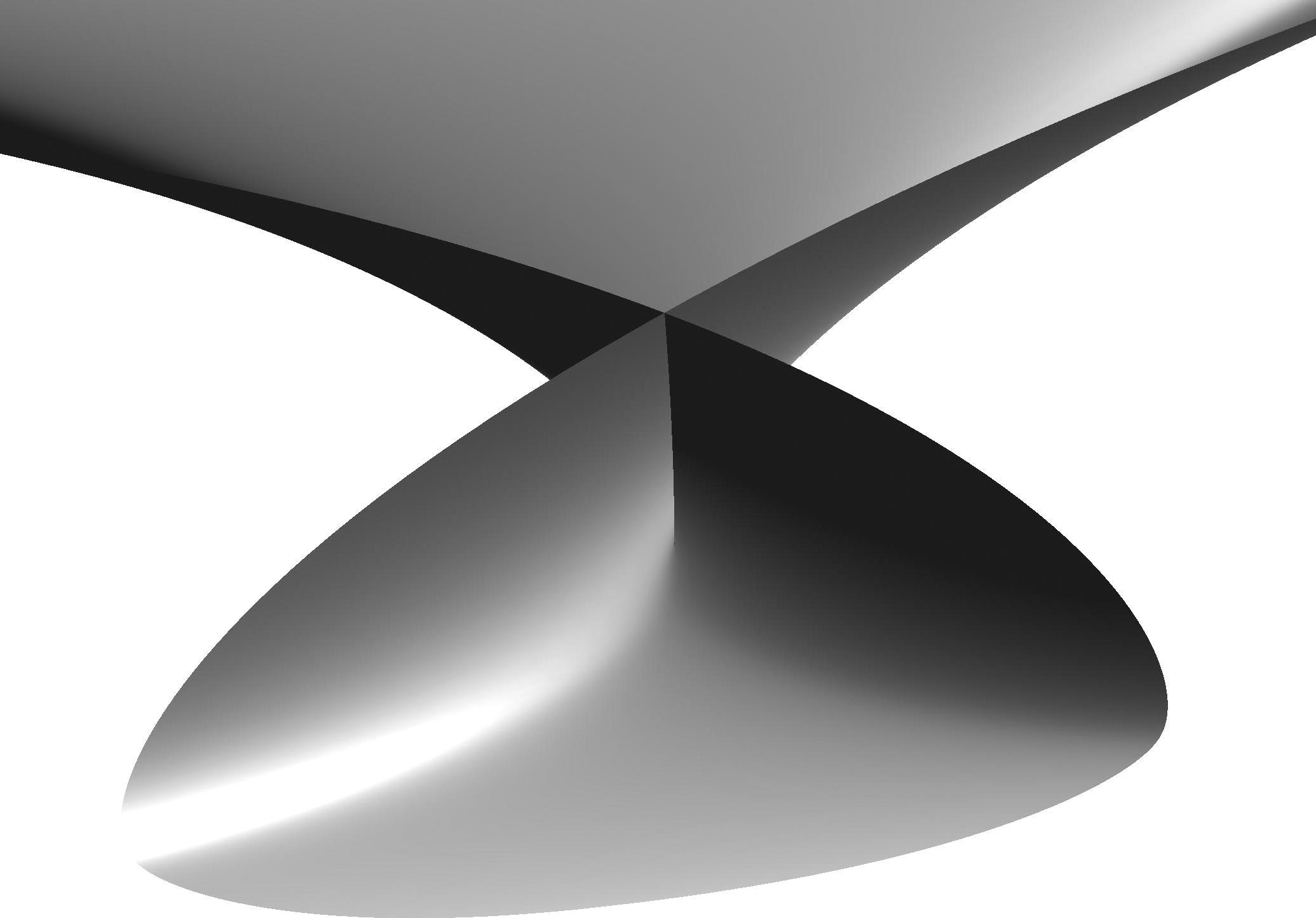
Figure 1. Numerical plots of solutions to the geometric Cauchy problem. Left: $s(v)=2+0.2v^{2}$, $t(v)=v$ (cuspidal cross cap). Right: $s(v)=v$, $t(v)=1$ (swallowtail).

In the last two sections we consider non-generic singularities. In Section 7 we solve the geometric Cauchy problem for characteristic data, where there are infinitely many solutions. The singular curve is always a straight line in this case. In Section 8 we compute numerically some examples of degenerate singularities.

In conclusion, we remark that the results of this article, combined with the results on Riemannian harmonic maps in [2, 4], ought to give a good indication of the typical situation at the big cell boundary for surfaces associated to harmonic or Lorentzian harmonic maps.

Notation: If $\hat{X}$ is a map into a loop group or loop algebra, we will sometimes use $X^{\lambda}$ for the corresponding group or algebra valued map $\hat{X}\big{|}_{\lambda}$, obtained by evaluating at a particular value $\lambda$ of the loop parameter. We also use $X:=X^{1}$. We use $\langle\cdot,\cdot\rangle_{E}$ and $\langle\cdot,\cdot\rangle_{L}$ for Euclidean and Lorentzian inner products respectively. We use $O(\lambda^{k})$ for an expression $g(\lambda)$ such that $\lim_{\lambda\to 0}g(\lambda)/\lambda^{k}$ is finite, and $O_{\infty}(\lambda^{k})$ for the anlogue when $\lambda\to\infty$.

2. Background material

We give a brief summary of the method given by Dorfmeister, Inoguchi and Toda [6] for constructing all timelike CMC surfaces from pairs of functions of one variable. The conventions we will use are mostly the same as those we used in [5], and the reader is therefore referred to that article for more details of the following sketch.

2.1. Loop groups

Let $\mathcal{G}=\Lambda\mathrm{SL}(2,{\mathbb{C}})_{\sigma\rho}$ be the group of loops in $\mathrm{SL}(2,{\mathbb{C}})$, with loop parameter $\lambda$, that are fixed by the commuting involutions

$$(\rho\gamma)(\lambda)=\overline{\gamma(\bar{\lambda})},\quad(\sigma\gamma)(\lambda)=\operatorname{Ad}_{P}\gamma(-\lambda),\quad P=\textup{diag}(1,-1).$$

The group $\mathcal{G}$ is a real form of $\mathcal{G}^{\mathbb{C}}=\Lambda\mathrm{SL}(2,{\mathbb{C}})_{\sigma}$, the group of loops fixed by $\sigma$.

Let $\Lambda^{\pm}\mathrm{SL}(2,{\mathbb{C}})_{\sigma}$ denote the subgroup of $\mathcal{G}^{\mathbb{C}}$ consisting of loops that extend holomorphically to ${\mathbb{D}}^{\pm}$, where ${\mathbb{D}}^{+}$ is the unit disc and ${\mathbb{D}}^{-}={\mathbb{S}}^{2}\setminus\{{\mathbb{D}}^{+}\cup{\mathbb{S}}^{1}\}$, the exterior disc in the Riemann sphere. Define

$$\mathcal{G}^{\pm}=\mathcal{G}\cap\Lambda^{\pm}\mathrm{SL}(2,{\mathbb{C}})_{\sigma},\quad\mathcal{G}^{+}_{*}=\{\gamma\in\mathcal{G}^{+}\ |\ \gamma(0)=I\},\quad\mathcal{G}^{-}_{*}=\{\gamma\in\mathcal{G}^{-}\ |\ \gamma(\infty)=I\}.$$

We define the complex versions $\mathcal{G}^{{\mathbb{C}}\pm}$ analogously by substituting $\mathcal{G}^{\mathbb{C}}$ for $\mathcal{G}$ in the above definitions.

The essential tool from loop groups needed is the Birkhoff decomposition, due to Pressley and Segal [17]. See [3] for a more general statement which includes the following case:

Theorem 2.1 (The Birkhoff decomposition).

The sets $\mathcal{B}_{L}=\mathcal{G}^{-}\cdot\mathcal{G}^{+}$ and $\mathcal{B}_{R}=\mathcal{G}^{+}\cdot\mathcal{G}^{-}$ are both open and dense in $\mathcal{G}$. The multiplication maps

$$\mathcal{G}^{-}_{*}\times\mathcal{G}^{+}\to\mathcal{B}_{L}\ \text{ and }\ \mathcal{G}^{+}_{*}\times\mathcal{G}^{-}\to\mathcal{B}_{R}$$

are both real analytic diffeomorphisms.

Note that the analogue also holds, substituting $\mathcal{G}^{\mathbb{C}}$, $\mathcal{G}^{{\mathbb{C}}\pm}$ and $\mathcal{G}^{{\mathbb{C}}\pm}_{*}$ for $\mathcal{G}$, $\mathcal{G}^{\pm}$ and $\mathcal{G}^{\pm}_{*}$, respectively, writing $\mathcal{B}_{L}^{\mathbb{C}}=\mathcal{G}^{{\mathbb{C}}-}\cdot\mathcal{G}^{{\mathbb{C}}+}$ and $B_{R}^{\mathbb{C}}=\mathcal{G}^{{\mathbb{C}}+}\cdot\mathcal{G}^{{\mathbb{C}}-}$.

The basis of the loop group approach is that timelike CMC surfaces correspond to a particular type of map into $\mathcal{G}$:

Definition 2.2.

Let $M$ be a simply connected open subset of ${\mathbb{R}}^{2}$, and let $(x,y)$ denote the standard coordinates. An admissible frame on $M$ is a smooth map $\hat{F}:M\to\mathcal{G}$ such that the Maurer-Cartan form of $\hat{F}$ is a Laurent polynomial in $\lambda$ of the form:

$$\hat{F}^{-1}\textup{d}\hat{F}=\lambda\,A_{1}\,\textup{d}x+\alpha_{0}+\lambda^{-1}A_{-1}\,\textup{d}y,$$

where the $\mathfrak{sl}(2,{\mathbb{R}})$-valued 1-form $\alpha_{0}$ is constant in $\lambda$. The admissible frame $\hat{F}$ is said to be regular if the components $[A_{1}]_{21}$ and $[A_{-1}]_{12}$ are non-vanishing.

2.2. Timelike CMC surfaces as admissible frames

We identify the Lie algebra $\mathfrak{sl}(2,{\mathbb{R}})$ with Lorentz-Minkowski space $\mathbb{L}^{3}$, with basis:

$$e_{0}=\begin{pmatrix}0&-1\\ 1&0\end{pmatrix}, e_{1}=\begin{pmatrix}0&1\\ 1&0\end{pmatrix}, e_{2}=\begin{pmatrix}-1&0\\ 0&1\end{pmatrix},$$

which are orthonormal with respect to the inner product $\langle X,Y\rangle_{L}=\frac{1}{2}\operatorname{trace}(XY)$, and with $\langle e_{0},e_{0}\rangle_{L}=-1$.

Let $M$ be a simply connected domain in ${\mathbb{R}}^{2}$, and $f:M\to\mathbb{L}^{3}$ a timelike immersion. The induced metric determines a Lorentz conformal structure on $M$. For any lightlike (also called null) coordinate system $(x,y)$ on $M$, we define a function $\omega:M\to{\mathbb{R}}$ by the condition that the induced metric is given by

$$\textup{d}s^{2}=\varepsilon e^{\omega}\,\textup{d}x\,\textup{d}y,\hskip 28.45274pt\varepsilon=\pm 1.$$

Let $N$ be a unit normal field for the immersion $f$, and define a coordinate frame for $f$ to be a map $F:M\to\mathrm{SL}(2,{\mathbb{R}})$ which satisfies

$$f_{x}=\dfrac{\varepsilon_{1}}{2}e^{\omega/2}\operatorname{Ad}_{F}(e_{0}+e_{1}),\quad f_{y}=\dfrac{\varepsilon_{2}}{2}e^{\omega/2}\operatorname{Ad}_{F}(-e_{0}+e_{1}),\quad N=\operatorname{Ad}_{F}(e_{2}),$$

where $\varepsilon_{1},\varepsilon_{2}\in\{-1,1\}$, so that $\textup{d}s^{2}$ is as above with $\varepsilon=\varepsilon_{1}\varepsilon_{2}$. Conversely, since $M$ is simply connected, we can always construct a coordinate frame for a timelike conformal immersion $f$.

The Maurer-Cartan form $\alpha$ for the frame $F$ is defined by

$$\alpha=F^{-1}\textup{d}F=U\textup{d}x+V\textup{d}y=A_{1}\textup{d}x+\alpha_{0}+A_{-1}\textup{d}y,$$

where $A_{\pm 1}$ are off-diagonal and $\alpha_{0}$ is a diagonal matrix valued 1-form. Let $\textup{Lie}(X)$ denote the Lie algebra of any group $X$. We extend $\alpha$ to a $\textup{Lie}(\mathcal{G})$-valued $1$-form $\hat{\alpha}$ by inserting the paramater $\lambda$ as follows:

$$\hat{\alpha}=A_{1}\lambda\textup{d}x+\alpha_{0}+A_{-1}\lambda^{-1}\textup{d}y,$$

where $\lambda$ is the complex loop parameter. The surface $f$ is of constant mean curvature if and only if $\hat{\alpha}$ satisfies the Maurer-Cartan equation $\textup{d}\hat{\alpha}+\hat{\alpha}\wedge\hat{\alpha}=0$, and one can then integrate the equation $\hat{F}^{-1}\textup{d}\hat{F}=\hat{\alpha}$, with $\hat{F}(0)=I$, to obtain the extended coordinate frame $\hat{F}:M\to\mathcal{G}$, which is a regular admissible frame.

It is important to note that the $1$-forms $A_{1}\textup{d}x$, $A_{-1}\textup{d}y$ and $\alpha_{0}$ are well-defined, independently of the choice of (oriented) lightlike coordinates, because any other lightlike coordinate system with the same orientation is given by $(\tilde{x}(x,y),\tilde{y}(x,y))=(\tilde{x}(x),\tilde{y}(y))$. This means that the extension of $F$ to $\hat{F}$ does not depend on coordinates.

One can reconstruct the surface $f$ as follows: define the map $\mathcal{S}:\Lambda\mathrm{SL}(2,{\mathbb{C}})\to\Lambda\mathfrak{sl}(2,{\mathbb{C}})$,

$$\mathcal{S}(\hat{G})=2\lambda\partial_{\lambda}\hat{G}\hat{G}^{-1}-\operatorname{Ad}_{\hat{G}}(e_{2}).$$

For any $\lambda_{0}\neq 0$, define $\mathcal{S}_{\lambda_{0}}(\hat{G})=\mathcal{S}(\hat{G})\big{|}_{\lambda=\lambda_{0}}$. Assume coordinates are chosen such that $f(p)=0$ for some point $p\in M$. Then $f$ is recovered by the Sym formula

$$f(z)=\frac{1}{2H}\left\{\mathcal{S}_{1}(\hat{F}(z))-\mathcal{S}_{1}(\hat{F}(p))\right\}.\\$$

Conversely, every regular admissible frame gives a timelike CMC surface: first note that a regular admissible frame can be written $\hat{F}^{-1}\textup{d}\hat{F}=\hat{U}\textup{d}x+\hat{V}\textup{d}y$, with

$$\hat{U}=\begin{pmatrix}a_{1}&b_{1}\lambda\\ c_{1}\lambda&-a_{1}\end{pmatrix}\quad\text{ and }\quad\hat{V}=\begin{pmatrix}a_{2}&b_{2}\lambda^{-1}\\ c_{2}\lambda^{-1}&-a_{2}\end{pmatrix}.$$

where $c_{1}$ and $b_{2}$ are non-zero.

Proposition 2.3.

Let $\hat{F}:M\to\mathcal{G}$ be a regular admissible frame and $H\neq 0$. Set $\varepsilon_{1}=\mathrm{sign}(c_{1})$, $\varepsilon_{2}=-\mathrm{sign}(b_{2})$ and $\varepsilon=\varepsilon_{1}\varepsilon_{2}$. Define a Lorentz metric on $M$ by

$$\textup{d}s^{2}=\varepsilon e^{\omega}\textup{d}x\,\textup{d}y,\quad\varepsilon e^{\omega}=-\dfrac{4c_{1}b_{2}}{H^{2}}.$$

Set

$$f^{\lambda}=\frac{1}{2H}\mathcal{S}_{\lambda}(\hat{F}):M\to\mathbb{L}^{3}\qquad(\lambda\in{\mathbb{R}}\setminus\{0\}).$$

Then, with respect to the choice of unit normal $N^{\lambda}=\operatorname{Ad}_{\hat{F}}e_{2}$, and the given metric, the surface $f^{\lambda}$ is a timelike CMC $H$-surface. Set

$$\rho=\left|\frac{b_{2}}{c_{1}}\right|^{\frac{1}{4}},\qquad T=\begin{pmatrix}\rho&0\\ 0&\rho^{-1}\end{pmatrix},$$

and set $\hat{F}_{C}=\hat{F}T:M\to\mathcal{G}$. Then $\hat{F}_{C}$ is the extended coordinate frame for the surface $f=f^{1}$. For general values of $\lambda\in{\mathbb{R}}\setminus\{0\}$ we have:

(2.1) $$\begin{split}f^{\lambda}_{x}=&\frac{\lambda c_{1}\rho^{2}}{H}\operatorname{Ad}_{F^{\lambda}_{C}}(e_{1}+e_{0})=\frac{\lambda\varepsilon_{1}e^{\omega/2}}{2}\operatorname{Ad}_{F^{\lambda}_{C}}(e_{1}+e_{0}),\\ f^{\lambda}_{y}=&\frac{b_{2}\rho^{-2}}{\lambda H}\operatorname{Ad}_{F^{\lambda}_{C}}(e_{1}-e_{0})=\frac{\varepsilon_{2}e^{\omega/2}}{2\lambda}\operatorname{Ad}_{F^{\lambda}_{C}}(e_{1}-e_{0}),\\ N^{\lambda}=&\operatorname{Ad}_{F^{\lambda}_{C}}e_{2}=\operatorname{Ad}_{F^{\lambda}}e_{2},\end{split}$$

where $N^{\lambda}$ is the unit normal to $f^{\lambda}$.

2.3. The d’Alembert type construction

We now explain how to construct all admissible frames, and thereby all timelike CMC surfaces, from simple data.

Definition 2.4.

Let $I_{x}\subset{\mathbb{R}}$ and $I_{y}\subset{\mathbb{R}}$ be open sets, with coordinates $x$ and $y$, respectively. A potential pair $(\psi^{X},\psi^{Y})$ is a pair of smooth $\textup{Lie}(\mathcal{G})$-valued 1-forms on $I_{x}$ and $I_{y}$ respectively with Fourier expansions in $\lambda$ as follows:

$$\psi^{X}=\sum_{j=-\infty}^{1}\psi^{X}_{i}\lambda^{i}\textup{d}x,\qquad\psi^{Y}=\sum_{j=-1}^{\infty}\psi^{Y}_{i}\lambda^{i}\textup{d}y.$$

The potential pair is called regular at a point $(x,y)$ if $[\psi^{X}_{1}]_{21}(x)\neq 0$ and $[\psi^{Y}_{-1}]_{12}(y)\neq 0$, and semi-regular if at most one of these functions vanishes at $(x,y)$, and the zero is of first order. The pair is called regular or semi-regular if the corresponding property holds at all points in $I_{x}\times I_{y}$.

The following theorem is a straightforward consequence of Theorem 2.1. Note that the potential pair in Item 1 of the theorem is well defined, independent of the choice of lightlike coordinates:

Theorem 2.5.

1. Let $M$ be a simply connected subset of ${\mathbb{R}}^{2}$ and $\hat{F}:M\to\mathcal{B}\subset\mathcal{G}$ an admissible frame. The pointwise (on $M$) Birkhoff decomposition

   $$\hat{F}=\hat{Y}_{-}\hat{H}_{+}=\hat{X}_{+}\hat{H}_{-},$$

   where $\hat{Y}_{-}(y)\in\mathcal{G}^{-}_{*}$, $\hat{X}_{+}(x)\in\mathcal{G}^{+}_{*}$, and $\hat{H}_{\pm}(x,y)\in\mathcal{G}^{\pm}$, results in a potential pair $(\hat{X}_{+}^{-1}\textup{d}\hat{X}_{+}\,,\,\hat{Y}_{-}^{-1}\textup{d}\hat{Y}_{-})$, of the form

   $$\hat{X}_{+}^{-1}\textup{d}\hat{X}_{+}=\psi^{X}_{1}\lambda\,\textup{d}x,\qquad\hat{Y}_{-}^{-1}\textup{d}\hat{Y}_{-}=\psi^{Y}_{-1}\lambda^{-1}\,\textup{d}y.\\$$

2. Conversely, given any potential pair, $(\psi^{X},\psi^{Y})$, define $\hat{X}:I_{x}\to\mathcal{G}$ and $\hat{Y}:I_{y}\to\mathcal{G}$ by integrating the differential equations

   $$\hat{X}^{-1}\textup{d}\hat{X}=\psi^{X}, \hat{X}(x_{0})=I,$$

   $$\hat{Y}^{-1}\textup{d}\hat{Y}=\psi^{Y}, \hat{Y}(y_{0})=I.$$

   Define $\hat{\Phi}=\hat{X}^{-1}\hat{Y}:I_{x}\times I_{y}\to\mathcal{G}$, and set $M=\hat{\Phi}^{-1}(\mathcal{B}_{L})$. Pointwise on $M$, perform the Birkhoff decomposition $\hat{\Phi}=\hat{H}_{-}\hat{H}_{+}$, where $\hat{H}_{-}:M\to\mathcal{G}^{-}_{*}$ and $\hat{H}_{+}:M\to\mathcal{G}^{+}$. Then $\hat{F}=\hat{Y}\hat{H}_{+}^{-1}$ is an admissible frame.
   

3. In both items (1) and (2), the admissible frame is regular if and only if the corresponding potential pair is regular. Moreover, with notation as in Definitions 2.2 and 2.4, we have $\textup{sign}[A_{1}]_{21}=\textup{sign}[\psi^{X}_{1}]_{21}$ and $\textup{sign}[A_{-1}]_{12}=\textup{sign}[\psi^{Y}_{-1}]_{12}$. In fact, we have

   (2.2) $$\hat{F}^{-1}\textup{d}\hat{F}=\lambda\psi^{X}_{1}\textup{d}x+\alpha_{0}+\lambda^{-1}\hat{H}_{+}\big{|}_{\lambda=0}\psi^{Y}_{-1}\hat{H}_{+}^{-1}\big{|}_{\lambda=0}\textup{d}y,$$

   where $\alpha_{0}$ is constant in $\lambda$.
   

3. Frontals and fronts

For the rest of this article we will be interested in timelike CMC surfaces with singularities. An appropriate class of generalized surface is a frontal. Here we briefly outline some definitions and results from [15] and [11].

Let $M$ be a $2$-dimensional manifold. A map $f:M\to{\mathbb{E}}^{3}$, into the three-dimensional Euclidean space, is called a frontal if, on a neighbourhood $U$ of any point of $M$, there exists a unit vector field ${\bf n}_{E}:U\to{\mathbb{S}}^{2}$, well-defined up to sign, such that ${\bf n}_{E}$ is perpendicular to $\textup{d}f(TM)$ in ${\mathbb{E}}^{3}$. The map $L=(f,\,[{\bf n}_{E}]):M\to{\mathbb{E}}^{3}\times{\mathbb{R}}P^{2}$ is called a Legendrian lift of $f$. If $L$ is an immersion, then $f$ is called a front. A point $p\in M$ where a frontal $f$ is not an immersion is called a singular point of $f$.

Suppose that the restriction of a frontal $f$, to some open dense set, is an immersion, and some Legendrian lift $L$ of $f$ is given. Then, around any point in $M$, there exists a smooth function $\chi$, given in local coordinates $(x,y)$ by the Euclidean inner product $\chi=\langle(f_{x}\times f_{y}),{\bf n}_{E}\rangle_{E}$, such that

$$f_{x}\times f_{y}=\chi{\bf n}_{E}.$$

In this situation, a singular point $p$ is called non-degenerate if $\textup{d}\chi$ does not vanish there, and the frontal $f$ is called non-degenerate if every singular point is non-degenerate. The set of singular points is locally given as the zero set of $\chi$, and is a smooth curve (in the coordinate domain) around non-degenerate points. At such a point, $p$, there is a well-defined direction, that is a non-zero vector $\eta\in T_{p}M$, unique up to scale, such that $\textup{d}f(\eta)=0$, called the null direction.

3.1. The Euclidean unit normal

In order to use the framework above, we need the Euclidean unit normal to a CMC surface. The orthonormal basis, $e_{0}$, $e_{1}$, $e_{2}$ for $\mathbb{L}^{3}$ satisfy the commutation relations $[e_{0},e_{1}]=2e_{2}$, $[e_{1},e_{2}]=-2e_{0}$ and $[e_{2},e_{0}]=2e_{1}$. Defining the standard cross product on the vector space ${\mathbb{R}}^{3}=\mathbb{L}^{3}$, with $e_{0}\times e_{1}=e_{2}$, $e_{1}\times e_{2}=e_{0}$ and $e_{2}\times e_{0}=e_{1}$, we have the formula:

$$A\times B=-\frac{1}{2}\operatorname{Ad}_{e_{0}}[A,B].\\$$

From Proposition 2.3, the coordinate frame for a regular timelike surface associated to an admissible frame is $f_{x}=\varepsilon_{1}e^{\omega/2}\operatorname{Ad}_{F_{C}}(e_{0}+e_{1})/2$, $f_{y}=\varepsilon_{2}e^{\omega/2}\operatorname{Ad}_{F_{C}}(-e_{0}+e_{1})/2$ and $N=\operatorname{Ad}_{F_{C}}e_{2}=\operatorname{Ad}_{F}e_{2}.$ We can use these to compute the cross product

(3.1) $$f_{x}\times f_{y}=-\frac{e^{\omega}}{2}\varepsilon\operatorname{Ad}_{e_{0}}\operatorname{Ad}_{F_{C}}(e_{2})=-\frac{e^{\omega}}{2}\varepsilon\operatorname{Ad}_{e_{0}}N,$$

where $\varepsilon=\varepsilon_{1}\varepsilon_{2}$. This formula is valid provided the surface is regular, that is, $c_{1}\neq 0\neq b_{2}$. However, the formula $N=\operatorname{Ad}_{F}e_{2}$ is valid everywhere, and gives a smooth vector field on $M$. Therefore, we define the Euclidean unit normal ${\bf n}_{E}$ to $f$ to be

(3.2) $${\bf n}_{E}:=\frac{\operatorname{Ad}_{e_{0}}\operatorname{Ad}_{F}(e_{2})}{||\operatorname{Ad}_{F}(e_{2})||},$$

where $||\cdot||$ is the standard Euclidean norm on the vector space ${\mathbb{R}}^{3}$ representing $\mathbb{L}^{3}$. At points where the surface is regular, we have

$${\bf n}_{E}=-\varepsilon\frac{f_{x}\times f_{y}}{||f_{x}\times f_{y}||}.$$

For other values of $\lambda\in{\mathbb{R}}\setminus\{0\}$ one defines the analogue ${\bf n}_{E}^{\lambda}$ for $f^{\lambda}$, by replacing $F$ with $F^{\lambda}$.

4. Singularities of class I: On the big cell

We now want to study the singularities occurring on a timelike CMC surface produced from a semi-regular potential pair $(\psi^{X},\psi^{Y})$, as in Theorem 2.5.

We first consider the case that the map $\hat{\Phi}=\hat{X}^{-1}\hat{Y}$ takes values in the big cell $\mathcal{B}_{L}$. In this case, the formula (3.2) for ${\bf n}_{E}$ shows that the Euclidean unit normal is never lightlike, regardless of whether the surface is immersed or not. Conversely, we will later show that, for singularities occurring at the big cell boundary, the Euclidean normal is always lightlike; this is the geometric difference between the two cases, which we will call class I and class II respectively. We now consider the generic singularity of the first case.

Given a potential pair, $(\psi^{X},\psi^{Y})=(O_{\infty}(1)+\psi^{X}_{1}\lambda\,,\,\psi^{Y}_{-1}\lambda^{-1}+O(1))$, we can write

$$\psi^{X}_{1}:=\begin{pmatrix}0&\alpha\\ \beta&0\end{pmatrix},\quad\psi^{Y}_{-1}:=\begin{pmatrix}0&\gamma\\ \delta&0\end{pmatrix},$$

where $\alpha$ and $\beta$ are real and depend on $x$ only, and $\gamma$ and $\delta$ are real and depend on $y$ only. From the converse part of Theorem 2.5, we see that these functions are otherwise completely arbitrary. If $\hat{\Phi}$ takes values in $\mathcal{B}_{L}$, the surface $f=\frac{1}{2H}\mathcal{S}_{1}(\hat{F})$ will have singularities when either of $\beta$ or $\gamma$ are zero, and is immersed otherwise. Thus, for a semi-regular potential, for which at most one of these is allowed to vanish, and this to first order, a singularity occurs at $z_{0}=(x_{0},y_{0})$ if and only if $\beta(x_{0})=0$, $\frac{\textup{d}\beta}{\textup{d}x}(x_{0})\neq 0$ and $\gamma(y_{0})\neq 0$ (or the analogue, switching $y$ with $x$ and $\beta$ with $\gamma$). For the generic case, the function $\alpha$ is also non-zero at $z_{0}$.

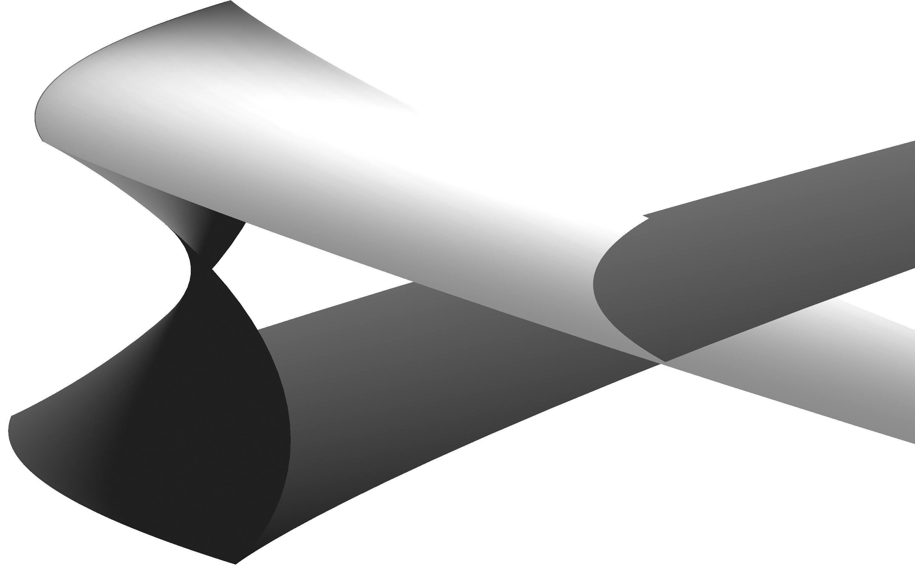
Figure 2. A numerical plot of a timelike CMC surface with cuspidal edges along the two coordinate lines $x=\pm 1$, produced by a pair of potentials with $\beta=(x-1)(x+1)$ and $\alpha=\gamma=\delta=1$.

We quote a characterization of the cuspidal edge from Proposition 1.3 in [15]:

Lemma 4.1.

Let $f$ be a front and $p$ a non-degenerate singular point. The image of $f$ in a neighbourhood of $p$ is diffeomorphic to a cuspidal edge if and only if the null direction $\eta(p)$ is transverse to the singular curve.

Now we can describe the generic singularities of a semi-regular surface on the big cell:

Proposition 4.2.

If the map $\hat{\Phi}=\hat{X}^{-1}\hat{Y}$ corresponding to a semi-regular potential pair takes values in $\mathcal{B}_{L}$, then a generic singularity of the surface $f:=\frac{1}{2H}\mathcal{S}_{1}(\hat{F})$ is a cuspidal edge.

Proof.

Clearly $(f,{\bf n}_{E})$ defines a frontal, where ${\bf n}_{E}$ is defined by equation (3.2). Assume now that, at $z_{0}=(0,0)$, we have $\beta=0$, $\frac{\textup{d}\beta}{\textup{d}x}\neq 0$ and $\alpha\neq 0$. Writing ${\bf n}_{E}=\mu\operatorname{Ad}_{e_{0}}\operatorname{Ad}_{F}e_{2}$, with $\mu=||\operatorname{Ad}_{F}e_{2}||^{-1}$, and examining the off-diagonal components in

$$\operatorname{Ad}_{F^{-1}}\operatorname{Ad}_{e_{0}}(\textup{d}{\bf n}_{E})=\mu[F^{-1}\textup{d}F,e_{2}]+\textup{d}\mu\,e_{2},$$

shows that ${\bf n}_{E}$ is an immersion. Hence the map $(f,{\bf n}_{E})$ is regular, and $f$ is a front.

To show that the singular point is non-degenerate we need to show that $\textup{d}\chi(z_{0})\neq 0$, where

$$\chi = \langle(f_{x}\times f_{y}),{\bf n}_{E}\rangle_{E}=-\dfrac{e^{\omega}}{2}\varepsilon\biggl{\langle}\operatorname{Ad}_{e_{0}}\operatorname{Ad}_{F}(e_{2}),\dfrac{\operatorname{Ad}_{e_{0}}\operatorname{Ad}_{F}(e_{2})}{||\operatorname{Ad}_{F}(e_{2})||}\biggr{\rangle}_{E}$$

$$= -\dfrac{\varepsilon e^{\omega}}{2}||\operatorname{Ad}_{F}(e_{2})||$$

$$= \dfrac{2b_{2}c_{1}}{H^{2}}||\operatorname{Ad}_{F}(e_{2})||,$$

in the notation of Proposition 2.3. Now using the expression (2.2) for $\hat{F}^{-1}\textup{d}\hat{F}$, we observe that $c_{1}=\beta$. Hence we obtain, at $(0,0)$,

$$\dfrac{\partial\chi}{\partial x}=\dfrac{\textup{d}\beta}{\textup{d}x}\dfrac{2b_{2}}{H^{2}}||\operatorname{Ad}_{F}(e_{2})||.$$

This is non-zero, since we assumed that $\frac{\textup{d}\beta}{\textup{d}x}\neq 0$, and, as mentioned in Theorem 2.5, $b_{2}$ vanishes if and only if $\gamma$ vanishes. Hence $\textup{d}\chi$ does not vanish at $(0,0)$.

According to Lemma 4.1, we need to show that the singular curve is transverse to the null direction. In a neighbourhood of $(0,0)$, the singular curve is given by the equation $x=0$, that is, it is tangent to $\partial_{y}$. Finally, since $f_{x}=0$ and $f_{y}\neq 0$ at $(0,0)$, the null direction at this point is $\eta(0)=\partial_{x}$.
∎

5. Singularities of class II: At the big cell boundary

We now turn to singularities that occur due to the failure of the loop group splitting at the boundary of the big cell. We again assume that the potentials corresponding to the surface are semi-regular at the points in question.

We need the Birkhoff decomposition of the whole group $\mathcal{G}^{\mathbb{C}}$:

Theorem 5.1.

[17, 4] Every element $\gamma\in\mathcal{G}^{\mathbb{C}}$ which is not in the left big cell $\mathcal{B}_{L}$ can be written as a product

$$\gamma=\gamma_{-}\,\omega\,\gamma_{+},$$

where $\gamma_{\pm}\in\mathcal{G}^{{\mathbb{C}}\pm}$ and the middle term $\omega$ is uniquely determined by $\gamma$ and has the form

$$\omega=\begin{pmatrix}\lambda^{2n}&0\\ 0&\lambda^{-2n}\end{pmatrix},\,\,n\in{\mathbb{Z}\setminus\{0\}},\,\,\,\textup{or}\,\,\,\omega=\begin{pmatrix}0&\lambda^{2n+1}\\ -\lambda^{-(2n+1)}&0\end{pmatrix},\,\,n\in{\mathbb{Z}}.$$

The same statement holds replacing $\mathcal{B}_{L}$ with $\mathcal{B}_{R}$ and interchanging $\gamma_{-}$ and $\gamma_{+}$.

We write

$$\omega_{k}=\begin{pmatrix}\lambda^{k}&0\\ 0&\lambda^{-k}\end{pmatrix}\ \ (\text{$k$ even}),\quad\omega_{k}=\begin{pmatrix}0&\lambda^{k}\\ -\lambda^{-k}&0\end{pmatrix}\ \ (\text{$k$ odd}),$$

and

$$\mathcal{P}_{L}^{k}=\{\gamma_{-}\,\omega_{k}\,\gamma_{+}\ |\ \gamma_{\pm}\in\mathcal{G}^{{\mathbb{C}}\pm}\}\qquad(k\in{\mathbb{Z}}).$$

We note that

$$\operatorname{Ad}_{e_{0}}(\mathcal{P}_{L}^{k})=\mathcal{P}_{L}^{-k}\ \ (\text{$k$ odd}),\qquad\operatorname{Ad}_{e_{1}}(\mathcal{P}_{L}^{k})=\mathcal{P}_{L}^{-k}\ \ (\text{$k$ even}).\\$$

5.1. Behaviour of the surface at $\mathcal{P}_{L}^{\pm 1}$ and $\mathcal{P}_{L}^{\pm 2}$.

The behaviour of the surface and its admissible frame at the smaller cells $\mathcal{P}_{L}^{\pm 1}$ and $\mathcal{P}_{L}^{\pm 2}$ is explained in the following result.

Theorem 5.2.

Let $\hat{X}:I_{x}\to\mathcal{G}$ and $\hat{Y}:I_{y}\to\mathcal{G}$ be obtained from a real analytic semi-regular potential pair as in Theorem 2.5. Set $M=I_{x}\times I_{y}$ and $\hat{\Phi}=\hat{X}^{-1}\hat{Y}$. Suppose that $M^{\circ}=\hat{\Phi}^{-1}(\mathcal{B}_{L})$ is non-empty. If for some $z_{0}=(x_{0},y_{0})\in M$, $\hat{\Phi}(z_{0})=\omega_{j}$ for $j=\pm 1$ or $\pm 2$, then

1. $M^{\circ}$ is open and dense in $M$;
   

2. if $j=1$, then the surface $f^{\lambda}:M^{\circ}\to\mathbb{L}^{3}$ obtained as $f^{\lambda}=\frac{1}{2H}\mathcal{S}_{\lambda}(\hat{F})$, for $\lambda\in{\mathbb{R}}\setminus\{0\}$, where $\hat{F}=\hat{Y}\hat{H}_{+}^{-1}$ as in Theorem 2.5, extends continuously to $z_{0}$, is real analytic in a neighbourhood of $z_{0}$, but is not immersed at $z_{0}$; moreover, the Euclidean unit normal is lightlike at $z_{0}$;
   

3. if $j=-1$, or $2$, then $\lim_{z\to z_{0}}\|f^{\lambda}\|=\infty$, where the limit is over values $z\in M^{\circ}$;
   

4. if $j=-2$ then $\lim_{z\to z_{0}}\|f^{\lambda}\|$ may be finite or infinite, depending on the sequence $z\to z_{0}$, but $f$ is not an immersed timelike surface at $z_{0}$.
   

Remark 5.3.

In the statement of the theorem, the assumption that the potential pair is real analytic is only used in item (1). By adding (1) as an assumption, (2), (3) and (4) still remain true (replacing real analytic with smooth in (2)) if the potential pair is only assumed smooth.

To prove the theorem we need two lemmas, both of which are verified by simple algebra.

Lemma 5.4.

Let $H_{-}=\begin{pmatrix}a&b\\ c&d\end{pmatrix}\in\mathcal{G}_{-}$.

1. If $c_{-1}\neq 0$, then $\omega_{1}H_{-}\in\mathcal{B}_{L}$ has a left Birkhoff decomposition

   $$\omega_{1}\hat{H}_{-}=\begin{pmatrix}\lambda c&\lambda d-u_{0}\lambda^{2}c\\ -\lambda^{-1}a&u_{0}a-\lambda^{-1}b\end{pmatrix}\begin{pmatrix}1&u_{0}\lambda\\ 0&1\end{pmatrix},$$

   where $u_{0}=d_{0}/c_{-1}$.

2. If $c_{-1}=0$, then $\omega_{1}\hat{H}_{-}\in\mathcal{P}_{L}^{1}$ has a left Birkhoff decomposition

   $$\omega_{1}\hat{H}_{-}=\begin{pmatrix}d&-\lambda^{2}c\\ -\lambda^{-2}b&a\end{pmatrix}\omega_{1}.$$

3. If $b_{-1}\neq 0$ then $\omega_{-1}\hat{H}_{-}\in\mathcal{B}_{L}$ has a left Birkhoff factorization

   $$\omega_{-1}\hat{H}_{-}=\begin{pmatrix}\lambda^{-1}c-v_{0}d&\lambda^{-1}d\\ -\lambda a+\lambda^{2}bv_{0}&-\lambda b\end{pmatrix}\begin{pmatrix}1&0\\ \lambda v_{0}&1\end{pmatrix},$$

   where $v_{0}=a_{0}/b_{-1}$.

4. If $b_{-1}=0$, then $\omega_{-1}\hat{H}_{-}\in\mathcal{P}_{L}^{-1}$ has a left Birkhoff decomposition

   $$\omega_{-1}\hat{H}_{-}=\begin{pmatrix}d&-\lambda^{-2}c\\ -\lambda^{2}b&a\end{pmatrix}\omega_{-1}.\\$$

Lemma 5.5.

Let $\hat{H}_{-}=\begin{pmatrix}a&b\\ c&d\end{pmatrix}\in\mathcal{G}_{-}$. Suppose that $b_{-1}\neq 0$ and $a_{-2}b_{-1}-a_{0}b_{-3}\neq 0$. Then $\omega_{2}\hat{H}_{-}\in\mathcal{B}_{L}$ has a left Birkhoff factorization $\omega_{2}\hat{H}_{-}=G_{-}G_{+}\,$, where

$$G_{+}=\begin{pmatrix}1+\dfrac{a_{0}b_{-1}}{a_{-2}b_{-1}-a_{0}b_{-3}}\lambda^{2}&\dfrac{b_{-1}^{2}}{a_{-2}b_{-1}-a_{0}b_{-3}}\lambda\vspace{1ex}\\ \dfrac{a_{0}}{b_{-1}}\lambda&1\end{pmatrix}.$$

Proof of Theorem 5.2.

Item (1): The big cell $\mathcal{B}_{L}$ is the complement of the zero set of a holomorphic section in a line bundle over the complex loop group [7]. Thus $M^{\circ}$ is the complement of the zero set of a real analytic section of the pull-back of this bundle by $\hat{\Phi}$. Since we have assumed that this set is non-empty, it must be open and dense.

Item (2): On $M^{\circ}$, we perform a left normalized Birkhoff decomposition $\hat{\Phi}=\hat{H}_{-}\hat{H}_{+}$. Since $\omega_{1}^{-1}\hat{\Phi}$ takes values in $\mathcal{B}_{L}$ in a neighbourhood $U$ of $z_{0}$, we perform a left normalized Birkhoff decomposition $\omega_{1}^{-1}\hat{\Phi}=\hat{G}_{-}\hat{G}_{+}$ in $U$. Thus, in $M^{\circ}\cap U$, we have $\hat{H}_{-}\hat{H}_{+}=\omega_{1}\hat{G}_{-}G_{+}$. Applying Lemma 5.4 to

$$\hat{G}_{-}=\begin{pmatrix}a&b\\ c&d\end{pmatrix},$$

gives

$$\hat{H}_{-}\hat{H}_{+}=\omega_{1}\hat{G}_{-}\hat{G}_{+}=\begin{pmatrix}\lambda c&\lambda d-\lambda^{2}\dfrac{c}{c_{-1}}\\ -\lambda^{-1}a&\dfrac{a}{c_{-1}}-\lambda^{-1}b\end{pmatrix}\begin{pmatrix}1&\dfrac{1}{c_{-1}}\lambda\\ 0&1\end{pmatrix}\hat{G}_{+}.$$

By uniqueness of the normalized Birkhoff factorization, we see that

$$\hat{H}_{-}=\omega_{1}\hat{G}_{-}\hat{U}_{+}^{-1}D^{-1},\quad\quad\hat{H}_{+}=D\hat{U}_{+}\hat{G}_{+},$$

where

$$\hat{U}_{+}=\begin{pmatrix}1&\dfrac{1}{c_{-1}}\lambda\\ 0&1\end{pmatrix},\qquad D=\begin{pmatrix}c_{-1}&0\\ 0&\dfrac{1}{c_{-1}}\end{pmatrix}.$$

Then

(5.1) $$\mathcal{S}_{\lambda}(\hat{F})=\mathcal{S}_{\lambda}(\hat{Y}\hat{H}_{+}^{-1})=\mathcal{S}_{\lambda}(\hat{Y}\hat{G}_{+}^{-1}\hat{U}_{+}^{-1}D^{-1})=\mathcal{S}_{\lambda}(\hat{Y}\hat{G}_{+}^{-1}),$$

because $\mathcal{S}_{\lambda}$ is invariant under postmultiplication by matrices of the form $\hat{U}_{+}$ and $D$ . Setting $\tilde{F}:=\hat{Y}\hat{G}_{+}^{-1}$, which is well defined and analytic in a neighbourhood of $z_{0}$, we have just shown that $\mathcal{S}_{\lambda}(\tilde{F})=\mathcal{S}_{\lambda}(\hat{F})$ on the intersection of their domains of definition. Hence $f^{\lambda}$ is well defined and analytic around $z_{0}$.

To see that $f^{\lambda}$ is not immersed at $z_{0}$, we have by Theorem 2.5,

$$\hat{F}^{-1}\textup{d}\hat{F}=\lambda\psi^{X}_{1}\textup{d}x+\alpha_{0}+\hat{H}_{+}\big{|}_{\lambda=0}\,\psi^{Y}_{-1}\hat{H}_{+}^{-1}\big{|}_{\lambda=0}\,\lambda^{-1}\textup{d}y.$$

We can write $\hat{G}_{+}=\textup{diag}(A_{0}\,,\,A_{0}^{-1})+O(\lambda)$. Then $\hat{H}_{+}=\textup{diag}(c_{-1}A_{0}\,,\,(c_{-1}A_{0})^{-1})+O(\lambda)$. Hence, if

$$\psi^{X}_{1}=\begin{pmatrix}0&\beta\\ \gamma&0\end{pmatrix},\quad\psi^{Y}_{-1}=\begin{pmatrix}0&\delta\\ \sigma&0\end{pmatrix},$$

then

$$\hat{H}_{+}\big{|}_{\lambda=0}\psi^{Y}_{-1}\hat{H}_{+}^{-1}\big{|}_{\lambda=0}=\begin{pmatrix}0&(c_{-1}A_{0})^{2}\delta\\ \dfrac{\sigma}{(c_{-1}A_{0})^{2}}&0\end{pmatrix}.$$

As the potential is semi-regular, $\gamma$ and $\delta$ do not vanish simultaneously, and their zeros are of first order, and therefore isolated. At points where these functions are non-zero, we set, as in Proposition 2.3,

$$\rho=\bigg{|}\dfrac{(c_{-1}A_{0})^{2}\delta}{\gamma}\bigg{|}^{1/4}\ \text{ and }\ T=\begin{pmatrix}\rho&0\\ 0&\rho^{-1}\end{pmatrix}$$

and $\hat{F}_{C}=\hat{F}T$. We have $\hat{F}=\hat{Y}\hat{H}_{+}^{-1}=\hat{Y}\hat{G}_{+}^{-1}\hat{U}_{+}^{-1}D^{-1}$, hence, by the formulae (2.1),

$$f^{\lambda}_{x} = \dfrac{\lambda\gamma\rho^{2}}{H}\operatorname{Ad}_{F^{\lambda}_{C}}(e_{0}+e_{1})=\dfrac{\lambda\gamma}{H}\operatorname{Ad}_{F}^{\lambda}(e_{0}+e_{1})$$

$$= \dfrac{\lambda\gamma}{H}\operatorname{Ad}_{Y^{\lambda}(G^{\lambda})_{+}^{-1}}((c_{1}^{2}+1)e_{0}+(c_{-1}^{2}-1)e_{1}-2c_{-1}e_{2}).$$

The last expression is well-defined and smooth, even at a point where $\gamma$ or $\delta$ vanishes, and therefore valid everywhere. Similarly,

$$f^{\lambda}_{y}=\dfrac{(c_{-1}A_{0})^{2}\delta\rho^{-2}}{\lambda H}\operatorname{Ad}_{F^{\lambda}_{C}}(e_{0}-e_{1})=\dfrac{A_{0}^{2}\delta}{\lambda H}\operatorname{Ad}_{Y^{\lambda}(G^{\lambda}_{+})^{-1}}(e_{0}-e_{1}).$$

As $A_{0}\to 1$ and $c_{-1}\to 0$ when $z\to z_{0}$, we have

(5.2) $$\begin{split}f^{\lambda}_{x}(z_{0})=\frac{\lambda\gamma}{H}\operatorname{Ad}_{Y^{\lambda}(G^{\lambda}_{+})^{-1}}(e_{0}-e_{1}),\\ f^{\lambda}_{y}(z_{0})=\frac{\delta}{\lambda H}\operatorname{Ad}_{Y^{\lambda}(G_{+}^{\lambda})^{-1}}(e_{0}-e_{1}).\end{split}$$

Thus we have proved that $f^{\lambda}$ is not immersed at $z_{0}$.

To see that the Euclidean normal is lightlike, see the explicit formula given below in Lemma 6.3. Alternatively, one can first show that the Minkowski unit normal $N^{\lambda}$ blows up (and therefore is asymptotically lightlike) by considering the surface $f^{\lambda}_{P}$ obtained from $\operatorname{Ad}_{e_{1}}\hat{F}$, which (one computes from the Sym formula) is the parallel surface to $f^{\lambda}$. Since $\operatorname{Ad}_{e_{1}}\hat{\Phi}(z_{0})=\omega_{-1}$, we show below that $f^{\lambda}_{P}$ blows up, and therefore so does $N^{\lambda}$. Hence the formula $(\ref{enormaldef})$ for the Euclidean normal shows that ${\bf n}_{E}^{\lambda}$ is lightlike at $z_{0}$.

Item (3): As in item (2), we write $\omega_{-1}^{-1}\hat{\Phi}=\hat{G}_{-}\hat{G}_{+}$ in a neighbourhood $U$ of $z_{0}$, and $\hat{\Phi}=H_{-}H_{+}$ in $U\cap M^{\circ}$. Again denoting the components of $\hat{G}_{-}$ by $a$, $b$, $c$ and $d$, Lemma 5.4 says that $\hat{H}_{+}=D\hat{U}_{+}\hat{G}_{+}$, where now

$$D=\begin{pmatrix}-b_{-1}^{-1}&0\\ 0&-b_{-1}\end{pmatrix},\qquad\hat{U}_{+}=\begin{pmatrix}1&0\\ \lambda b_{-1}^{-1}&1\end{pmatrix}.$$

Hence

$$2Hf^{\lambda}=\mathcal{S}_{\lambda}(\hat{Y}\hat{G}_{+}^{-1}\hat{U}_{+}^{-1})=\operatorname{Ad}_{Y^{\lambda}(G^{\lambda}_{+})^{-1}}(\mathcal{S}_{1}(\hat{U}_{+}^{-1}))+\mathcal{S}_{1}(\hat{Y}\hat{G}_{+}^{-1}).$$

Since $\hat{Y}\hat{G}_{+}^{-1}$ are well defined and real analytic in $U$, the second term is finite in $U$, while the first term is given by

$$\operatorname{Ad}_{Y^{\lambda}(G^{\lambda}_{+})^{-1}}(\mathcal{S}_{1}(\hat{U}_{+}^{-1}))=-2b_{-1}^{-1}\operatorname{Ad}_{Y^{\lambda}(G^{\lambda}_{+})^{-1}}(e_{0}+e_{1})-\operatorname{Ad}_{Y^{\lambda}(G^{\lambda}_{+})^{-1}}e_{2}.$$

The second term is finite in $U$, while the first term goes to infinity as $z\to z_{0}$, since $b_{-1}\to 0$ in this case. This proves item (3) for $j=-1$.

If $\hat{\Phi}(z_{0})=\omega_{2}$, we proceed as in the case just described, choosing a suitable neighbourhood $U$ of $z_{0}$ and write $\omega_{2}^{-1}\hat{\Phi}=\omega_{2}^{-1}\hat{H}_{-}\hat{H}_{+}=\hat{G}_{-}\hat{G}_{+}$ on $U\cap M^{\circ}$. Using the same notation for the components of $\hat{G}_{-}$, we have by Lemma 5.5, $\hat{H}_{+}=D\hat{U}_{+}\hat{G}_{+}$, where $D$ is a diagonal matrix constant in $\lambda$, and

$$\hat{U}_{+}=\begin{pmatrix}1+\dfrac{b_{-1}}{a_{-2}b_{-1}-b_{-3}}\lambda^{2}&\dfrac{b_{-1}^{2}}{a_{-2}b_{-1}-b_{-3}}\lambda\\ \dfrac{1}{b_{-1}}\lambda&1\end{pmatrix}.$$

We have

$$2Hf^{\lambda}=\mathcal{S}_{1}(\hat{Y}\hat{G}_{+}^{-1}\hat{U}_{+}^{-1}D^{-1})=\operatorname{Ad}_{Y^{\lambda}(G^{\lambda}_{+})^{-1}}\left(\mathcal{S}_{1}(\hat{U}_{+}^{-1}))+\mathcal{S}_{1}(\hat{Y}\hat{G}_{+}^{-1})\right).$$

The second term is finite, while the first term is given by

$$\operatorname{Ad}_{Y^{\lambda}(G^{\lambda}_{+})^{-1}}\mathcal{S}_{1}(\hat{U}_{+}^{-1}))=-2b_{-1}^{-1}\operatorname{Ad}_{Y^{\lambda}(G^{\lambda}_{+})^{-1}}(e_{0}+e_{1})-\operatorname{Ad}_{Y^{\lambda}(G^{\lambda}_{+})^{-1}}e_{2},$$

and the conclusion follows as in the case when $j=-1$.

Item (4): The case when $j=-2$ can be computed in an analogous way to $j=2$. Instead of the equation above, one is led to:

$$\operatorname{Ad}_{Y^{\lambda}(G^{\lambda}_{+})^{-1}}\mathcal{S}_{1}(\hat{U}_{+}^{-1}))=\operatorname{Ad}_{Y^{\lambda}(G^{\lambda}_{+})^{-1}}\begin{pmatrix}4\Delta\lambda^{2}&4\Delta c_{-1}^{-1}\lambda^{3}\\ -4c_{-1}\Delta\lambda&-4\Delta\lambda^{2}\end{pmatrix}-\operatorname{Ad}_{Y^{\lambda}(G^{\lambda}_{+})^{-1}}e_{2},$$

where $\Delta=c_{-1}/(d_{-2}c_{-1}-c_{-3})$, and the functions $c_{-1}$, $d_{-2}$ and $c_{-3}$ all approach zero as $z\to z_{0}$. Since it is possible to choose sequences such that the right hand side of the above equation is either finite or infinite as $z\to z_{0}$, we can say nothing about this limit. If the limit is finite, we can deduce that the map $f$ is not an immersion as follows: by the same argument described above for $j=1$, namely considering the surface $f_{P}^{\lambda}$, which blows up, since $f_{P}^{\lambda}(z_{0})\in\mathcal{P}_{L}^{2}$, one deduces that the Minkowski normal must be lightlike at $z_{0}$. This cannot happen on an immersed timelike surface.
∎

Note that generic singularities should not occur at points in $\mathcal{P}_{L}^{j}$ for $|j|>1$, because the codimension of the small cells in the loop group increases with $|j|$. In view of the previous theorem, and with the aim of studying surfaces with finite, generic singularities, we make the following definition:

Definition 5.6.

A generalized timelike CMC $H$ surface is a smooth map $f:\Sigma\to\mathbb{L}^{3}$, from an oriented surface $\Sigma$, such that, at every point $z_{0}$ in $\Sigma$, the following holds: there exists a neighbourhood $U$ of $z_{0}$ such that the restriction $f\big{|}_{U}$ can be represented by a semi-regular potential pair $(\psi^{X},\psi^{Y})$, where the corresponding map $\hat{\Phi}=\hat{X}^{-1}\hat{Y}$ maps $U$ into $\mathcal{B}_{L}\cup\mathcal{P}_{L}^{1}$, and where $\hat{\Phi}^{-1}(\mathcal{B}_{L})$ is open and dense in $U$. If the potential pair is regular, the surface is called weakly regular.

Note that if $f$ is weakly regular, that is, represented by a regular potential pair at each point, then $f$ is immersed precisely at those points for which the corresponding map $\hat{\Phi}$ maps into the big cell $\mathcal{B}_{L}$. In other words, there is a well defined open dense set $\Sigma^{\circ}$ on which $f$ is an immersion and $f$ will have singularities precisely at points which map into $\mathcal{P}_{L}^{1}$.

6. Prescribing class II singularities of non-characteristic type

We have seen that the Euclidean unit normal ${\bf n}_{E}$ is well defined at a singularity occurring on the big cell. Below we will show that this is also the case for those at the big cell boundary. Then we have seen in the previous sections that singularities in the two cases can be distinguished by the property that ${\bf n}_{E}$ is not lightlike in the first case, and is lightlike in the second case, which we have already named class I and class II respectively.

Constructing surfaces with a prescribed singular curve of the class I is simple: it is a matter of solving the geometric Cauchy problem for the characteristic case (see [5]), which has infinitely many solutions, and choosing the second potential to be non-regular at the point in question. Therefore, we henceforth discuss only singularities of class II.

6.1. Singular potentials

Assume now that we are at a non-degenerate singular point $p=f(0,0)$, so that the pre-image of the singular set in a neighbourhood of $p$ is given by some curve $\Gamma:(\alpha,\beta)\to M$. Assume that $\Gamma$ is never parallel to a lightlike coordinate line $y=\textup{constant}$ or $x=\textup{constant}$, which means that the singular curve is non-characteristic for the associated PDE. The characteristic case will be discussed in the next section.

With the non-characteristic assumption, one can express $\Gamma$ as a graph, $y=h(x)$, with $h^{\prime}(x)$ non-vanishing, and, after a change of coordinates $(\tilde{x},\tilde{y})=(h(x),y)$, which are still lightlike coordinates for the regular part of the surface, one can even assume that $\Gamma$ is given by $y=x$, which is to say $u=0$ in the coordinates

$$u=\frac{1}{2}\left(x-y\right),\hskip 28.45274ptv=\frac{1}{2}\left(x+y\right).$$

Note that we could distinguish the cases $h^{\prime}>0$ and $h^{\prime}<0$, which corresponds to the curve being spacelike/timelike in the coordinate domain, but nothing fundamentally new is gained by doing this.

The issues discussed below are local in nature, and therefore we assume that our parameter space is a square, $M=J\times J\subset{\mathbb{R}}^{2}$, where $J$ is an open interval containing $0$. In these coordinates, along the line $y=x=v$ we have, by definition of $\mathcal{P}_{L}^{1}$,

$$\hat{\Phi}(v)=\hat{X}^{-1}(v)\hat{Y}(v)=\hat{G}_{-}(v)\,\omega_{1}\,\hat{G}_{+}(v),$$

with $\hat{G}_{-}(v)\in\mathcal{G}^{-}$ and $\hat{G}_{+}(v)\in\mathcal{G}^{+}$. It is also easy to show, using the expressions in Lemma 5.4, that if $\hat{\Phi}$ is smooth then $\hat{G}_{-}$ and $\hat{G}_{+}$ can also be chosen to be smooth. We can replace the map $\hat{X}(x)$ by $\hat{X}(x)\hat{G}_{-}(x)$, and $\hat{Y}(y)$ by $\hat{Y}(y)\hat{G}_{+}^{-1}(y)$, which correspond to the standard potential pair

$$\psi^{X}=\hat{G}_{-}^{-1}(\hat{X}^{-1}\textup{d}\hat{X})\hat{G}_{-}+\hat{G}_{-}^{-1}\textup{d}\hat{G}_{-},$$

$$\psi^{Y}=\hat{G}_{+}(\hat{Y}^{-1}\textup{d}\hat{Y})\hat{G}_{+}^{-1}+\hat{G}_{+}\textup{d}\hat{G}_{+}^{-1},$$

and it is simple to check that the surface constructed from these potentials is the same as the original surface. Thus one can, in fact, assume that

$$\hat{\Phi}(v)=\hat{X}^{-1}(v)\hat{Y}(v)=\omega_{1}.\\$$

Finally, choosing a normalization point $z_{0}=(0,0)$ on the singular set, one can also assume that

$$\hat{X}(z_{0})=\omega_{1}^{-1},\quad\hat{Y}(z_{0})=I.$$

This is achieved by premultiplying both $\hat{Y}$ and $\hat{X}$ by $\hat{Y}^{-1}(z_{0})$. This leaves $\hat{\Phi}$ unchanged, and alters the surface $f=(1/2H)\mathcal{S}_{1}(\hat{Y}\hat{H}_{+}^{-1})$ of Theorem 2.5 only by an isometry consisting of conjugation by $Y^{-1}(z_{0})$ plus a translation.

As shown by equation (5.1) in Theorem 5.2, we can equivalently consider the map $\tilde{\Phi}:=\omega_{1}^{-1}\hat{\Phi}$, which is the same as replacing $\hat{X}$ by $\tilde{X}:=\hat{X}\omega_{1}$. Therefore, we first look at the Maurer-Cartan form of $\tilde{X}$, given that $\hat{X}^{-1}\textup{d}\hat{X}$ is a standard potential of the form:

$$\begin{pmatrix}\alpha_{0}+O_{\infty}(\lambda^{-2})&\beta_{1}\lambda+\beta_{-1}\lambda^{-1}\beta_{-3}\lambda^{-3}+O_{\infty}(\lambda^{-5})\\ \gamma_{1}\lambda+\gamma_{-1}\lambda^{-1}+\gamma_{-3}\lambda^{-3}+O_{\infty}(\lambda^{-5})&-\alpha_{0}+O_{\infty}(\lambda^{-2})\end{pmatrix}\textup{d}x.$$

Then

$$\tilde{X}^{-1}\textup{d}\tilde{X} = \omega_{1}^{-1}(\hat{X}^{-1}\textup{d}\hat{X}^{-1})\omega_{1}$$

$$= \begin{pmatrix}-\alpha_{0}&-\gamma_{1}\lambda^{3}-\gamma_{-1}\lambda-\gamma_{-3}\lambda^{-1}\\ -\beta_{1}\lambda^{-1}&\alpha_{0}\end{pmatrix}\textup{d}x+O_{\infty}(\lambda^{-2}).$$

Now we observe that, since $\tilde{X}^{-1}(v)Y(v)=I$ for all $v$, we actually have

$$\tilde{X}(v)=Y(v)$$

for all $v$. It follows that, along $y=x$, we have $\tilde{X}^{-1}\textup{d}\tilde{X}=\psi^{Y}$, which was assumed to be a standard potential, and so all the terms of order $-2$ or lower in $\lambda$ are zero.

Definition 6.1.

A singular potential on an open interval $J\subset{\mathbb{R}}$, is a $\textup{Lie}(\mathcal{G})$-valued 1-form $\tilde{\psi}$ on $J$ which has the Fourier expansion in $\lambda$:

$$\tilde{\psi}=\begin{pmatrix}-\alpha_{0}&-\gamma_{1}\lambda^{3}-\gamma_{-1}\lambda-\gamma_{-3}\lambda^{-1}\\ -\beta_{1}\lambda^{-1}&\alpha_{0}\end{pmatrix}\textup{d}v=:A(v)\textup{d}v.$$

Any zeros of $\gamma_{1}$ and $\gamma_{-3}$ are of at most first order. The potential is regular at points where $\gamma_{1}$ and $\gamma_{-3}$ do not vanish. The potential is non-degenerate at points where $\beta_{1}$ does not vanish.

We have seen by the above argument that a timelike CMC surface that has a non-degenerate singular point gives us a singular potential $\tilde{\psi}(v)=A(v)\textup{d}v$, and moreover is reconstructed, up to an isometry of the ambient space, by integrating $\tilde{X}^{-1}\textup{d}\tilde{X}(x)=A(x)\textup{d}x$ and $\hat{Y}^{-1}\textup{d}\hat{Y}(y)=A(y)\textup{d}y$, both with initial condition the identity, Birkhoff splitting $\tilde{\Phi}=\tilde{X}^{-1}\hat{Y}=\hat{G}_{-}\hat{G}_{+}$ and setting $f=(1/2H)\mathcal{S}_{1}(\hat{Y}\hat{G}_{+}^{-1})$. Conversely, we have the following:

Proposition 6.2.

Let $\tilde{\psi}(v)$ be a singular potential which is non-degenerate along $J$. Integrate $\tilde{X}^{-1}\textup{d}\tilde{X}=\tilde{\psi}$, with initial condition the identity, to obtain a map, $\tilde{X}:J\to\mathcal{G}$. Define $\tilde{\Phi}:J\times J\to\mathcal{G}$ by

$$\tilde{\Phi}(x,y):=\tilde{X}^{-1}(x)\hat{Y}(y),\quad\hat{Y}(y):=\tilde{X}(y).$$

Let $\lambda\in{\mathbb{R}}\setminus\{0\}$.

1. Set $\hat{\Phi}:=\omega_{1}\tilde{\Phi}$. Then the set $\Sigma^{\circ}:=\hat{\Phi}^{-1}(\mathcal{B}_{L})$ is non-empty. The map $f^{\lambda}:\Sigma^{\circ}\to\mathbb{L}^{3}$ obtained from $\hat{\Phi}$ as in Theorem 2.5 is a timelike CMC surface, regular at points where $\tilde{\psi}$ is regular.
   

2. Let $\Delta:=\{(x,x)~{}|~{}x\in J\}\subset J\times J$. The set $\Sigma_{s}:=\Sigma^{\circ}\cup\Delta$ is open in $J\times J$, and the map $f^{\lambda}$ extends to a map $\Sigma_{s}\to\mathbb{L}^{3}$ as follows: Set $U:=\Sigma_{s}\cap\tilde{\Phi}^{-1}(\mathcal{B}_{L})$, which is an open set containing $\Delta$. On $U$ perform the pointwise left normalized Birkhoff factorization $\tilde{\Phi}=\hat{G}_{-}\hat{G}_{+}$. Set

   $$f^{\lambda}:=\mathcal{S}_{\lambda}(\hat{Y}\hat{G}_{+}^{-1}).$$

   The extended map $f^{\lambda}:\Sigma_{s}\to\mathbb{L}^{3}$ is a generalized timelike CMC $H$ surface. Moreover $\Delta$ is contained in the singular set, and is equal to the singular set if the potential is regular.
   

3. Along $\Delta$, we have the expressions

   (6.1) $$f^{\lambda}_{x}=\lambda\dfrac{\gamma_{1}}{H}\operatorname{Ad}_{Y^{\lambda}}(e_{0}-e_{1}),\quad f^{\lambda}_{y}=-\dfrac{1}{\lambda}\dfrac{\gamma_{-3}}{H}\operatorname{Ad}_{Y^{\lambda}}(e_{0}-e_{1}).\\$$

Proof.

Item (1): We need to show that $\hat{\Phi}^{-1}(\mathcal{B}_{L})$ is non-empty. The rest of the statement then follows from Theorem 5.2. Factorizing $\tilde{\Phi}=\tilde{X}^{-1}\hat{Y}=\hat{G}_{-}\hat{G}_{+}$ as in item (2) around $\Delta$, and writing

$$\hat{G}_{-}=O_{\infty}(\lambda^{-2})+\begin{pmatrix}1&b_{-1}\lambda^{-1}\\ c_{-1}\lambda^{-1}&1\end{pmatrix},\quad\quad\hat{G}_{+}=\begin{pmatrix}A_{0}&B_{1}\lambda\\ C_{1}\lambda&A_{0}^{-1}\end{pmatrix}+O(\lambda^{2}),$$

we recall from the proof of Theorem 5.2 that $\hat{\Phi}:=\omega_{1}\hat{G}_{-}\hat{G}_{+}$ is in the big cell if and only if $c_{-1}\neq 0$. Thus we need to show that $c_{-1}$ is non-zero away from $\Delta$, for which it is enough to show that the derivative of $c_{-1}$ is non-zero along $\Delta$. Differentiating $\tilde{X}^{-1}\hat{Y}=\hat{G}_{-}\hat{G}_{+}$ and evaluating along $\Delta$, along which $\hat{G}_{-}=\hat{G}_{+}=I$, we have

$$-\tilde{X}^{-1}\textup{d}\tilde{X}+\hat{Y}^{-1}\textup{d}\hat{Y}=\textup{d}\hat{G}_{-}+\textup{d}\hat{G}_{+}.$$

Using that $\tilde{X}$ is a function of $x$ only and $\hat{Y}$ is a function of $y$, and that they take the same value along $x=y=v$, this becomes

$$\textup{d}\hat{G}_{-}+\textup{d}\hat{G}_{+} = -A\textup{d}x+A\textup{d}y$$

$$= -2A\textup{d}u.$$

Comparing the coefficients of $\lambda^{-1}$, $\lambda^{0}$ and $\lambda$, we conclude that, for $x=y=v$,

(6.2) $$\textup{d}\hat{G}_{-}=\begin{pmatrix}0&2\gamma_{-3}\\ 2\beta_{1}&0\end{pmatrix}\lambda^{-1}\textup{d}u,\quad\quad\textup{d}\hat{G}_{+}=2\begin{pmatrix}\alpha_{0}&\gamma_{-1}\lambda+\gamma_{1}\lambda^{3}\\ 0&-\alpha_{0}\end{pmatrix}\textup{d}u.$$

Thus, $\textup{d}c_{-1}=2\beta_{1}\textup{d}u$, and the condition that $\beta_{1}$ does not vanish guarantees that $\partial_{u}c_{-1}$ is non-vanishing on $\Delta$.

Item (2): Follows from Theorem 5.2.

Item (3): This is (5.2) of Theorem 5.2, substituting $\gamma=\gamma_{1}$, $\delta=-\gamma_{3}$, since the potentials $\psi^{X}$ and $\psi^{Y}$ referred to there are here represented by $\psi^{X}=\hat{X}^{-1}\textup{d}\hat{X}=\omega_{1}\tilde{\psi}\omega_{1}^{-1}$ and $\psi^{Y}=\tilde{\psi}$.
∎

6.2. Extending the Euclidean normal to the singular set

Let $f$ be a generalized timelike CMC $H$ surface. We earlier defined the Euclidean unit normal ${\bf n}_{E}:=\operatorname{Ad}_{e_{0}}\operatorname{Ad}_{F}(e_{2})/||\operatorname{Ad}_{F}(e_{2})||$, which is well defined on $\Sigma^{\circ}=\hat{\Phi}^{-1}(\mathcal{B}_{L})$. For a point $z_{0}\in\Sigma\setminus\Sigma^{\circ}=\hat{\Phi}^{-1}(\mathcal{P}_{L}^{1})$ one has, on some neighbourhood $U$ of $z_{0}$, that the singular set is locally given as the set $c_{-1}=0$, where $c$ is the $(2,1)$-component of $\hat{G}_{-}$ in the proof of Theorem 5.2. To extend ${\bf n}_{E}$ continuously over $\hat{\Phi}^{-1}(\mathcal{P}_{L}^{1})$, we need to multiply it by the sign of $c_{-1}$, and so we redefine it:

(6.3) $${\bf n}_{E}\,\,:=\,\,\mathrm{sign}(c_{-1})\frac{\operatorname{Ad}_{e_{0}}\operatorname{Ad}_{F}(e_{2})}{||\operatorname{Ad}_{F}(e_{2})||}\,\,=\,\,-\varepsilon\,\mathrm{sign}(c_{-1})\frac{f_{x}\times f_{y}}{\|f_{x}\times f_{y}\|},$$

where $\varepsilon=\varepsilon_{1}\varepsilon_{2}$ as before.

Lemma 6.3.

Let $f$ be a generalized timelike CMC surface, locally represented by $\hat{\Phi}=\hat{X}^{-1}\hat{Y}$, and let $z_{0}$ be a point such that $\hat{\Phi}(z_{0})=\omega_{1}$. Then ${\bf n}_{E}$ is well defined and smooth on a neighbourhood $U$ of $z_{0}$, and we have:

$${\bf n}_{E}=\frac{\operatorname{Ad}_{e_{0}}\operatorname{Ad}_{YG_{+}^{-1}}(c_{-1}e_{2}+e_{0}-e_{1})}{||\operatorname{Ad}_{YG_{+}^{-1}}(c_{-1}e_{2}+e_{0}-e_{1})||},$$

where $c_{-1}:U\to{\mathbb{R}}$ and $G_{+}:U\to\mathrm{SL}(2,{\mathbb{C}})$ are smooth, $c_{-1}(z_{0})=0$ and $G_{+}(z_{0})=I$.

Proof.

With notation as in the proof Theorem 5.2, we have

$$\hat{F}=\hat{Y}\hat{H}_{+}^{-1}=\hat{Y}\hat{G}_{+}^{-1}\hat{U}_{+}^{-1}D^{-1},$$

and

$$U_{+}^{-1}D^{-1}=\begin{pmatrix}c_{-1}^{-1}&-1\\ 0&c_{-1}\end{pmatrix},\quad\operatorname{Ad}_{U_{+}^{-1}D^{-1}}(e_{2})=c_{-1}^{-1}(c_{-1}e_{2}+e_{0}-e_{1}).$$

Substituting into the definition for ${\bf n}_{E}$ proves the lemma. ∎

Note that if $Y(z_{0})=I$ then this simplifies to ${\bf n}_{E}(z_{0})=(e_{0}+e_{1})/{\sqrt{2}}$.

Lemma 6.4.

Let $f$ be a generalized timelike CMC surface, locally represented by $\hat{\Phi}$, and let $z_{0}$ be a point such that $\hat{\Phi}(z_{0})=\omega_{1}$ and $\hat{Y}(z_{0})=I$. Then

$$\lim_{z\to z_{o}}\textup{d}{\bf n}_{E}(z)=-\frac{1}{\sqrt{2}}((\sigma+\beta)\textup{d}u+(\sigma-\beta)\textup{d}v)e_{2}.$$

where,

$$\psi^{X}=\left(O_{\infty}(1)+\begin{pmatrix}0&\beta\\ \gamma&0\end{pmatrix}\lambda\right)\textup{d}x,\quad\psi^{Y}=\left(\begin{pmatrix}0&\delta\\ \sigma&0\end{pmatrix}\lambda^{-1}+O(1)\right)\textup{d}y,$$

are a regular potential pair corresponding to the surface.

Proof.

As in Lemma 6.3, we have $\hat{F}=\hat{Y}\hat{H}_{+}^{-1}=\hat{Y}\hat{G}_{+}^{-1}\hat{U}_{+}^{-1}D^{-1}$. Differentiating ${\bf n}_{E}$ gives:

$$\textup{d}{\bf n}_{E}= \dfrac{\mathrm{sign}(c_{-1})}{\|\operatorname{Ad}_{F}(e_{2})\|}\operatorname{Ad}_{e_{0}}\biggl{(}\operatorname{Ad}_{F}[F^{-1}\textup{d}F,e_{2}]$$

$$-\dfrac{1}{\|\operatorname{Ad}_{F}(e_{2})\|^{2}}\langle\operatorname{Ad}_{F}[F^{-1}\textup{d}F,e_{2}],\operatorname{Ad}_{F}(e_{2})\rangle_{E}\operatorname{Ad}_{F}(e_{2})\biggr{)}.$$

According to Theorem 2.5 (3), we have

$$F^{-1}\textup{d}F=\psi^{X}_{1}\textup{d}x+\alpha_{0}+\hat{H}_{+}\big{|}_{\lambda=0}\psi^{Y}_{-1}\hat{H}_{+}^{-1}\big{|}_{\lambda=0},$$

where $\alpha_{0}$ is a diagonal matrix of $1$-forms. As in the proof of Theorem 5.2, we write

$$\psi^{X}_{1}=\begin{pmatrix}0&\beta\\ \gamma&0\end{pmatrix},\qquad\hat{H}_{+}\big{|}_{\lambda=0}\psi^{Y}_{-1}\hat{H}_{+}^{-1}\big{|}_{\lambda=0}=\begin{pmatrix}0&g^{2}\delta\\ g^{-2}\sigma&0\end{pmatrix},$$

where $g=c_{-1}A_{0}\to 0$ as $z_{0}$. Writing $c=c_{-1}$ to simplify notation, one obtains from $\operatorname{Ad}_{YG_{+}^{-1}}=I+o(1)$, the following formula:

$$\operatorname{Ad}_{F}[F^{-1}\textup{d}F,e_{2}]= 2\begin{pmatrix}c\gamma&\gamma+c^{-2}\beta\\ -c^{2}\gamma&-c\gamma\end{pmatrix}\textup{d}x$$

$$+2\begin{pmatrix}cg^{-2}\sigma g^{-2}\sigma+c^{-2}g^{2}\delta\\ -s_{-1}^{2}g^{-2}\sigma&-cg^{-2}\sigma\end{pmatrix}\textup{d}y+o(1).$$

Using that $\operatorname{Ad}_{F}(e_{2})=c^{-1}(e_{0}-e_{1})+e_{2}+o(1)$, we obtain

$$\begin{split}\langle\operatorname{Ad}_{F}[F^{-1}\textup{d}F,e_{2}],\operatorname{Ad}_{F}(e_{2})\rangle_{E}=&-2(c\gamma+c^{-1}(c^{-2}\beta+\gamma))\textup{d}x\\ &-2(cg^{-2}\sigma+c^{-1}(c^{-2}g^{2}\delta+g^{-2}\sigma))\textup{d}y+o(1),\end{split}$$

and so we have

$$\begin{split}\operatorname{Ad}_{e_{0}}(\textup{d}{\bf n}_{E})=&o(1)+\frac{1}{\sqrt{2}}\begin{pmatrix}c^{2}\gamma-c^{4}\gamma-\beta&2c^{2}\gamma-2c^{3}\gamma-2c\gamma\\ -2c^{2}\gamma&-c^{2}\gamma+c^{4}\gamma+\beta\end{pmatrix}\textup{d}x\\ &+\dfrac{c^{2}}{g^{2}\sqrt{2}}\begin{pmatrix}\dfrac{c^{2}}{g^{2}}\sigma-\dfrac{c^{4}}{g^{2}}\sigma+g^{2}\delta&-2g^{-2}\sigma\\ -2g^{-2}\sigma&-\dfrac{c^{2}}{g^{2}}\sigma+\dfrac{c^{4}}{g^{2}}\sigma+g^{2}\delta\end{pmatrix}\textup{d}y.\end{split}$$

As $z\to z_{0}$ we have $c\to 0$ and $g/c\to 1$; hence

$$\operatorname{Ad}_{e_{0}}(\textup{d}{\bf n}_{E})\to\frac{1}{\sqrt{2}}(\beta e_{2}\textup{d}x-\sigma e_{2}\textup{d}y)=\frac{1}{\sqrt{2}}((\beta+\sigma)\textup{d}u+(\beta-\sigma)\textup{d}v)e_{2}.$$

Since $\operatorname{Ad}_{e_{0}}(e_{2})=-e_{2}$, the result follows.
∎

Proposition 6.5.

Let $f$ be the surface constructed from a singular potential $\tilde{\psi}$ in accordance with Proposition 6.2. The map $f:\Sigma_{s}\to\mathbb{L}^{3}$ is a frontal. A singular point on $\hat{\Phi}^{-1}(\mathcal{P}_{L}^{1})$ is non-degenerate if and only if $\tilde{\psi}$ is non-degenerate and regular at the point.

Proof.

That $f$ is a frontal follows from Lemma 6.3. To show that the frontal is non-degenerate, we must show that $\textup{d}\chi\neq 0$ at a singular point $z_{0}$, where $f_{x}\times f_{y}=\chi{\bf n}_{E}$. By the definition (6.3), we have

$$\chi=-\varepsilon\mathrm{sign}(c_{-1})\|f_{x}\times f_{y}\|.$$

In the notation of Theorem 5.2 we have

$$\varepsilon\frac{e^{\omega}}{2}=\langle f_{x},f_{y}\rangle_{L}=-2\frac{\gamma\delta A_{0}^{2}c_{-1}^{2}}{H^{2}}.$$

Substituting into the expression (3.1) we obtain

$$\chi=-\varepsilon\mathrm{sign}(c_{-1})\frac{e^{\omega}}{2}\|\operatorname{Ad}_{F}(e_{2})\|=2\mathrm{sign}(c_{-1})\frac{\gamma\delta A_{0}^{2}c_{-1}^{2}}{H^{2}}\|\operatorname{Ad}_{F}(e_{2})\|.$$

The derivative is

$$\textup{d}\chi= \mathrm{sign}(c_{-1})\dfrac{\gamma\delta A_{0}^{2}}{H^{2}}\biggl{(}2c_{-1}^{2}\dfrac{\langle\operatorname{Ad}_{F}[F^{-1}\textup{d}F,e_{2}],\operatorname{Ad}_{F}(e_{2})\rangle_{E}}{\|\operatorname{Ad}_{F}(e_{2})\|}$$

$$+4c_{-1}\|\operatorname{Ad}_{F}(e_{2})\|\textup{d}c_{-1}\biggr{)}+o(1).$$

From the proof of Lemma 6.4 and the fact that $c_{-1}\|\operatorname{Ad}_{F}(e_{2})\|=\mathrm{sign}(c_{-1})\sqrt{2}+o(1)$, an easy calculation gives

$$c_{-1}^{2}\frac{\langle\operatorname{Ad}_{F}[F^{-1}\textup{d}F,e_{2}],\operatorname{Ad}_{F}(e_{2})\rangle_{E}}{\|\operatorname{Ad}_{F}(e_{2})\|}=-\sqrt{2}\mathrm{sign}(c_{-1})(\beta\textup{d}x+\sigma\textup{d}y)+o(1).$$

With our choice of potentials, we have

$$\beta=\beta_{1},\quad\gamma=\gamma_{1}\quad\sigma=-\beta_{1},\quad\delta=-\gamma_{-3},$$

so that ($\beta\textup{d}x+\sigma\textup{d}y)=2\beta_{1}\textup{d}u$. From (6.2) we have $\textup{d}c_{-1}=2\beta_{1}\textup{d}u$. Hence

$$\textup{d}\chi=-4\sqrt{2}\dfrac{\beta_{1}\gamma_{1}\gamma_{-3}}{H^{2}}\textup{d}u.$$

Hence the singular point is non-degenerate if and only if $\gamma_{1}$, $\gamma_{-3}$ and $\beta_{1}$ are non-zero, which is the condition that the potential is regular and non-degenerate.

∎

6.3. The singular geometric Cauchy problem

The goal of this section is to construct generalized timelike CMC surfaces with prescribed singular curves. As above, we assume the curve in the coordinate domain is non-characteristic, that is, never parallel to a coordinate line.

In order to obtain a unique solution, we need to specify the derivatives of $f$ as well, as follows:

Problem 6.6.

The (non-characteristic) singular geometric Cauchy problem: Let $J$ be a real interval with coordinate $v$. Given a smooth map $f_{0}:J\to\mathbb{L}^{3}$, and a vector field $V:J\to\mathbb{L}^{3}$ such that $f_{0}^{\prime}(v)$ is lightlike, $V$ is proportional to $f_{0}^{\prime}(v)$ and the two vector fields do not vanish simultaneously. Find a generalized timelike CMC surface $f:\Sigma\to\mathbb{L}^{3}$, where $\Sigma$ is some open subset of the $uv$-plane which contains the interval $J\subset\{u=0\}$, that, away from $J$, is conformally immersed with lightlike coordinates $x=u+v$, $y=-u+v$, and such that along $J$ the following hold:

$$\left.f\right|_{J}=f_{0},\quad\left.f_{u}\right|_{J}=V.$$

After an isometry of the ambient space, we can assume that $f_{0}^{\prime}(v)=s(v)(-e_{0}+\cos\theta(v)e_{1}+\sin\theta(v)e_{2})$, for some smooth functions $s$ and $\theta$, with $\theta(0)=0$, and so the derivatives of a solution $f$ must satisfy:

(6.4) $$\begin{split}f_{v}=s(-e_{0}+\cos\theta e_{1}+\sin\theta e_{2}),\\ f_{u}=t(-e_{0}+\cos\theta e_{1}+\sin\theta e_{2}),\end{split}$$

where $s$, $t$ are smooth and do not vanish simultaneously, and the function $t$ is deduced from $V$.

We want to construct a singular potential

$$\tilde{\psi}=\begin{pmatrix}-\alpha_{0}&-\gamma_{1}\lambda^{3}-\gamma_{-1}\lambda-\gamma_{-3}\lambda^{-1}\\ -\beta_{1}\lambda^{-1}&\alpha_{0}\end{pmatrix}\textup{d}v.$$

for the surface. Our task is to find $\gamma_{1}$, $\gamma_{\pm 1}$, $\gamma_{-3}$ and $\alpha_{0}$. We begin by looking for a "singular frame" $F_{0}=\tilde{X}\big{|}_{\lambda=1}=\hat{Y}\big{|}_{\lambda=1}$ along $y=x$, such that $F_{0}^{-1}\textup{d}F_{0}=\tilde{\psi}\big{|}_{\lambda=1}$. According to Proposition 6.2, using the formulae (6.1) for $f_{y}$ and $f_{x}$ along $\Delta$, we must have

$$f_{v} = \frac{1}{H}(-\gamma_{1}+\gamma_{-3})\operatorname{Ad}_{F_{0}}(e_{1}-e_{0}),$$

$$f_{u} = -\frac{1}{H}(\gamma_{1}+\gamma_{-3})\operatorname{Ad}_{F_{0}}(e_{1}-e_{0}).$$

Comparing with (6.4) a solution for $F_{0}$ is given by:

$$F_{0}=\begin{pmatrix}\cos(\theta/2)&-\sin(\theta/2)\\ \sin(\theta/2)&\cos(\theta/2)\end{pmatrix},$$

and with that choice of $F_{0}$, the functions $\gamma_{1}$ and $\gamma_{-3}$ are determined as:

$$\gamma_{1}=\frac{-H(s+t)}{2},\quad\gamma_{-3}=\frac{H(s-t)}{2}.\\$$

Next we have the expression

$$F_{0}^{-1}(F_{0})_{v}=\frac{\theta^{\prime}}{2}\begin{pmatrix}0&-1\\ 1&0\end{pmatrix}.$$

Comparing this with $\tilde{\psi}$, evaluated at $\lambda=1$, we obtain: $\alpha_{0}=0$, $\theta^{\prime}/2=-\beta_{1}$, and $\theta^{\prime}/2=\gamma_{1}+\gamma_{-1}+\gamma_{-3}$, and so:

$$\alpha_{0}=0,\quad\beta_{1}=-\frac{\theta^{\prime}}{2},\quad\gamma_{-1}=\frac{\theta^{\prime}}{2}+Ht.\\$$

Hence, provided that $\hat{\Phi}^{-1}(\mathcal{B}_{L})$ is not empty, a solution for the singular geometric Cauchy problem with data given by (6.4) is obtained from the singular potential,

$$\tilde{\psi}=\frac{1}{2}\begin{pmatrix}0&H(s+t)\lambda^{3}-\left(\theta^{\prime}+2Ht\right)\lambda+H(t-s)\lambda^{-1}\\ \theta^{\prime}\lambda^{-1}&0\end{pmatrix}\textup{d}v.$$

According to Proposition 6.5, the singular curve is non-degenerate if and only if the three functions $s+t$, $t-s$ and $\theta^{\prime}$ do not vanish. The non-degeneracy condition is thus:

$$s\neq\pm t\quad\textup{and}\quad\theta^{\prime}\neq 0.\\$$

Theorem 6.7.

The surface $f:J\times J\to\mathbb{L}^{3}$ obtained from the singular potential $\tilde{\psi}$ given above is the unique solution for the non-characteristic geometric Cauchy problem given by the equations (6.4).

Proof.

We know that any solution surface is given locally by the the construction in Proposition 6.2. So suppose we have another solution $\check{f}$, with corresponding singular potential $\check{\tilde{\psi}}$. From the formulae (6.1) for $f^{\lambda}_{x}$ and $f^{\lambda}_{y}$, we must have, along $\Delta$,

$$\gamma_{1}\operatorname{Ad}_{Y^{\lambda}}(e_{1}-e_{0})=\check{\gamma}_{1}\operatorname{Ad}_{\check{Y}^{\lambda}}(e_{1}-e_{0}).$$

We conclude that

$$\check{Y}^{\lambda}(y)=Y^{\lambda}(y)T^{\lambda}(y),$$

where $T^{\lambda}$ commutes, up to a scalar, with $(e_{1}-e_{0})$, and is therefore of the form

$$T^{\lambda}=\begin{pmatrix}\mu&\nu\\ 0&\mu^{-1}\end{pmatrix}.$$

Now computing $(\check{Y}^{\lambda})^{-1}\textup{d}\check{Y}^{\lambda}=\operatorname{Ad}_{T^{\lambda}}\tilde{\psi}+(T^{\lambda})^{-1}\textup{d}T^{\lambda}$, we obtain for the $(1,1)$ and $(2,1)$ components respectively:

$$-\check{\alpha}_{0}=-\alpha_{0}+\mu\nu\beta_{1}\lambda^{-1}+\mu^{-1}\textup{d}\mu,$$

$$-\check{\beta}_{1}\lambda^{-1}=-\mu^{2}\beta_{1}\lambda^{-1}.$$

It follows that

$$\mu=\mu_{0},\quad\nu=\nu_{1}\lambda,$$

where $\mu_{0}$ and $\nu_{1}$ are constant in $\lambda$.

Now the surface $f$ is obtained as $2Hf=\mathcal{S}_{1}\left(\hat{Y}\,\hat{G}_{+}^{-1}\right)$, where

(6.5) $$\hat{X}^{-1}\,\hat{Y}=\hat{G}_{-}\,\hat{G}_{+}$$

is a normalized Birkhoff factorization. Likewise, since $\hat{\check{Y}}=\hat{Y}\,\hat{T}$, and $\hat{\check{X}}(x)=\hat{\check{Y}}(x)=\hat{X}(x)\,\hat{S}(x)$, where we set $\hat{S}(x)=\hat{T}(x)$, the map $\check{f}$ is obtained as $2H\check{f}=\mathcal{S}_{1}(\hat{Y}\,\hat{T}\,\hat{\check{G}}_{+}^{-1})$, where

$$\hat{S}^{-1}\,\hat{X}^{-1}\,\hat{Y}\,\hat{T}=\hat{\check{G}}_{-}\,\hat{\check{G}}_{+}.$$

Now, inserting the Birkhoff factorization at (6.5), we have

$$\hat{\check{G}}_{-}\,\hat{\check{G}}_{+} = \hat{S}^{-1}\,\hat{G}_{-}\,\hat{G}_{+}\,\hat{T}$$

$$= \hat{H}_{-}\,\hat{D}_{+}\,\hat{G}_{+}\,\hat{T},$$

where $\hat{H}_{-}$ takes values in $\mathcal{G}_{*}^{-}$ and, writing $\hat{G}_{-}=\small{\begin{pmatrix}A&B\\ C&D\end{pmatrix}}$, we have, if $v\neq 0$,

$$\hat{D}_{+}=\begin{pmatrix}r&\lambda\\ 0&r^{-1}\end{pmatrix},\quad r=\frac{\mu_{0}A_{0}+\nu_{1}C_{-1}}{\nu_{0}D_{0}},$$

and $\hat{D}_{+}=\hat{S}$ if $\nu=0$. Since $\hat{T}$ takes values in $\mathcal{G}^{+}$, we conclude by uniqueness of the normalized Birkhoff factorization of $\hat{\check{G}}_{-}\,\hat{\check{G}}_{+}$ that

$$\hat{\check{G}}_{+}=\hat{D}_{+}\,\hat{G}_{+}\,\hat{T},$$

and

$$2H\check{f}(x,y) = \mathcal{S}_{1}\left(\hat{Y}\,\hat{T}\,\,\hat{T}^{-1}\hat{G}_{+}^{-1}\hat{D}_{+}^{-1}\right)$$

$$= \mathcal{S}_{1}\left(\hat{Y}\,\hat{G}_{+}^{-1}\hat{D}_{+}^{-1}\right)$$

$$= \mathcal{S}_{1}\left(\hat{Y}\,\hat{G}_{+}^{-1}\right),$$

because right multiplication by either of the candidates for $\hat{D}_{+}^{-1}$ leaves the Sym formula unchanged. Thus $\check{f}=f$, and the solution is unique.
∎

6.4. Generic singularities

The object of this section is to prove:

Theorem 6.8.

Let $f$ be a generalized timelike CMC surface, and $z_{0}$ a non-degenerate singular point. Assume that the singular curve is non-characteristic at $z_{0}$. By Theorem 6.7, we may assume that $f$ is locally represented by a singular potential:

$$\tilde{\psi}=\frac{1}{2}\begin{pmatrix}0&H(s+t)\lambda^{3}-\left(\theta^{\prime}+2Ht\right)\lambda+H(t-s)\lambda^{-1}\\ \theta^{\prime}\lambda^{-1}&0\end{pmatrix}\textup{d}v,$$

where $s$, $t$ and $\theta^{\prime}$ are the geometric Cauchy data described in that section, $z_{0}=(0,0)$, and $\tilde{X}(0)=\hat{Y}(0)=I$.

Then, at $z_{0}=(0,0)$, the surface is locally diffeomorphic to a :

1. cuspidal edge if and only if both $s(0)$ and $t(0)$ are nonzero,
   

2. swallowtail if and only if

   $$s(0)=0,\quad s^{\prime}(0)\neq 0,\quad t(0)\neq 0,\\$$

3. cuspidal cross cap if and only if

   $$t(0)=0,\quad t^{\prime}(0)\neq 0,\quad s(0)\neq 0.\\$$

Before proving this, we state conditions suitable for our context that characterize swallowtails, cuspidal edges and cuspidal cross caps:

Proposition 6.9.

[15]. Let $f:U\to{\mathbb{R}}^{3}$ be a front, and $p$ a non-degenerate singular point. Suppose that $\gamma:(-\delta,\delta)\to U$ is a local parameterization of the singular curve, with parameter $x$ and tangent vector $\dot{\gamma}$, and $\gamma(0)=p$. Then:

1. The image of $f$ in a neighbourhood of $p$ is diffeomorphic to a cuspidal edge if and only if $\eta(0)$ is not proportional to $\dot{\gamma}(0)$.

2. The image of $f$ in a neighbourhood of $p$ is diffeomorphic to a swallowtail if and only if $\eta(0)$ is proportional to $\dot{\gamma}(0)$ and

   $$\frac{\textup{d}}{\textup{d}x}\det\left(\dot{\gamma}(x),\eta(x)\right)\Big{|}_{x=0}\neq 0.$$

   
   

Theorem 6.10.

[11]. Let $f:U\to{\mathbb{R}}^{3}$ be a frontal, with Legendrian lift $L=(f,{\bf n}_{E})$, and let $z_{0}$ be a non-degenerate singular point. Let $Z:V\to{\mathbb{R}}^{3}$ be an arbitrary differentiable function on a neighbourhood $V$ of $z_{0}$ such that:

1. $Z$ is orthogonal to ${\bf n}_{E}$.

2. $Z(z_{0})$ is transverse to the subspace $\textup{d}f(T_{z_{0}}(V))$.
   

Let $x$ be the parameter for the singular curve, $\eta(x)$ a choice vector field for the null direction, and set

$$\tau(x):=\langle{\bf n}_{E},\textup{d}Z(\eta)\rangle_{E}\big{|}_{x}.$$

The frontal $f$ has a cuspidal cross cap singularity at $z=z_{0}$ if and only:

• $\eta(z_{0})$ is transverse to the singular curve;

• $\tau(z_{0})=0$ and $\tau^{\prime}(z_{0})\neq 0$.
  

Proof of Theorem 6.8.

First, note that $f$ is a front if and only if $t$ does not vanish, since, from Lemma 6.4 we have $\textup{d}{\bf n}_{E}\big{|}_{z=z_{0}}=-\sqrt{2}\theta^{\prime}/2\,\textup{d}v\,e_{2}$, and, from the geometric Cauchy construction, $\textup{d}f\big{|}_{z=z_{0}}=(s\textup{d}v+t\,\textup{d}u)(e_{1}-e_{0})$. Thus, writing $L=(f,{\bf n}_{E})$, we have

$$L_{u}=\left(t(e_{1}-e_{0}),\,0\right),\quad L_{v}=\left(s(e_{1}-e_{0}),\,-\frac{\sqrt{2}\theta^{\prime}}{2}e_{2}\right).$$

The curve is assumed non-degenerate, so $\theta^{\prime}\neq 0$, and therefore $L$ has rank $2$ at $z_{0}$ if and only if $t(0)\neq 0$.

The singular curve is given by $u=0$ and hence tangent to $\partial_{v}=\partial_{x}+\partial_{y}$, and the null direction is defined by the vector field $\eta=s\partial_{u}-t\partial_{v}$. Hence, by Proposition 6.9 the surface is locally diffeomorphic to a cuspidal edge around the singular point $z_{0}$ if and only if both $s$ and $t$ are non-zero. This proves item (1). To prove item (2), we just need to notice that $\det(\dot{\gamma},\eta)=-s$.

To prove item (3), we will choose a suitable vector field $Z$ and apply Theorem 6.10 above. We use the setup from Lemma 6.3, whence we see that the Euclidean normal around the singular point is parallel to

$$\operatorname{Ad}_{e_{0}}\operatorname{Ad}_{YG_{+}^{-1}}(e_{0}-e_{1}+c_{-1}e_{2}).$$

Furthermore, $f_{x}$ and $f_{y}$ are both parallel to $\operatorname{Ad}_{F_{0}}(e_{0}-e_{1})=\operatorname{Ad}_{e_{0}}\operatorname{Ad}_{F_{0}}(e_{0}+e_{1})$ along the singular curve. Thus, the vector field $Z$ defined by

$$Z=\operatorname{Ad}_{e_{0}}\operatorname{Ad}_{YG_{+}^{-1}}(e_{0}-e_{1}+c_{-1}e_{2})\times\operatorname{Ad}_{e_{0}}\operatorname{Ad}_{YG_{+}^{-1}}(e_{0}+e_{1}),$$

is orthogonal to the Euclidean normal in a neighbourhood of $z_{0}$ and transverse to $f_{x}$ and $f_{y}$ along the singular curve in this neighbourhood. From Section 3.1, we have $e_{0}\times e_{1}=e_{2}$, $e_{1}\times e_{2}=e_{0}$ and $e_{2}\times e_{0}=e_{1}$, and for any vectors $a$ and $b$ and matrix $X$ we have $(\operatorname{Ad}_{e_{0}}\operatorname{Ad}_{X}(a))\,\times\,(\operatorname{Ad}_{e_{0}}\operatorname{Ad}_{X}(b))=\operatorname{Ad}_{X}\operatorname{Ad}_{e_{0}}(a\times b)$. Thus,

$$Z= \operatorname{Ad}_{YG_{+}^{-1}}\operatorname{Ad}_{e_{0}}(c_{-1}(e_{1}-e_{0})+2e_{2})$$

$$= \operatorname{Ad}_{YG_{+}^{-1}}(-2e_{2}-c_{-1}(e_{1}+e_{0})).$$

Write $\tilde{\psi}=\hat{A}(v)\textup{d}v$, so that $\hat{Y}^{-1}\textup{d}\hat{Y}=\hat{A}(y)\textup{d}y$. Along the singular curve, where $c_{-1}=0$, we have

$$\textup{d}Z=-\operatorname{Ad}_{F_{0}}([A\,\textup{d}y-\textup{d}G_{+},2e_{2}]+(e_{0}+e_{1})\textup{d}c_{-1}).$$

From (6.2) with $\lambda=1$, we have

$$\textup{d}G_{+}=\frac{1}{2}(\theta^{\prime}+H(t-s))(e_{1}-e_{0})\textup{d}u,\quad\quad\textup{d}c_{-1}=-\theta^{\prime}\textup{d}u,$$

and we also have $A=\hat{A}\big{|}_{\lambda=1}=\theta^{\prime}e_{0}/2$.

Hence

$$(A\textup{d}y-\textup{d}G_{+})(\eta) = \frac{1}{2}(\theta^{\prime}e_{0}(\textup{d}v-\textup{d}u)-(\theta^{\prime}+H(t-s))(e_{1}-e_{0})\textup{d}u)(s\partial_{u}-t\partial v)),$$

$$= \frac{1}{2}\left((sH(t-2)-t\theta^{\prime})e_{0}-s(\theta^{\prime}+H(t-s))e_{1}\right),$$

and

$$\textup{d}c_{-1}(\eta)=-s\theta^{\prime}.\\$$

Putting all these together:

$$\textup{d}Z(\eta)\big{|}_{u=0}=-\operatorname{Ad}_{F_{0}}\left(s\left(2H(t-s)+\theta^{\prime}\right)(e_{0}-e_{1})+2t\theta^{\prime}e_{1}\right).$$

Along the singular curve the expression for ${\bf n}_{E}$ simplifies to

$${\bf n}_{E}=\frac{1}{\sqrt{2}}\operatorname{Ad}_{F_{0}}(e_{0}+e_{1}).$$

Since $F_{0}$ is in $\textup{SU}(2)$ and preserves the Euclidean inner product, we finally arrive at

$$\tau(v)=\langle{\bf n}_{E},\textup{d}Z(\eta)\rangle_{E}(0,v)=-\sqrt{2}t\theta^{\prime}.$$

Since $\theta^{\prime}\neq 0$, the condition (B) of Theorem 6.10 is equivalent to: $t=0$ and $t^{\prime}\neq 0$; finally, condition (A) is equivalent to: $s\neq 0$. This proves item (3).
∎

7. Prescribing class II singularities of characteristic type

Suppose now that we have a generalized timelike CMC surface with non-degenerate singular curve that is always tangent to a characteristic direction, that is, the curve is given in local lightlike coordinates $(x,y)$ as $y=0$.

If $\hat{X}$ and $\hat{Y}$ are the associated data, and the singularity is of class II, then we must have $\hat{\Phi}(x,0)=\hat{X}^{-1}(x)\,\hat{Y}(0)=\hat{H}_{-}(x)\omega_{1}\hat{H}_{+}(x)$, where $\hat{H}_{\pm}$ take values in $\mathcal{G}^{\pm}$. By a similar argument to that in Section 6.1, no generality is lost in assuming that $\hat{H}_{-}(x)=I$, and

$$\hat{X}(x)=\hat{H}_{+}(x)\omega_{1}^{-1},\quad\hat{H}_{+}(x)\in\mathcal{G}^{+},\quad\hat{H}_{+}(0)=I,\quad\hat{Y}(0)=I.$$

Now writing

$$\hat{X}^{-1}\textup{d}\hat{X}=(...+A_{-1}\lambda^{-1}+A_{0}+A_{1}\lambda)\textup{d}x,\quad\hat{H}_{+}^{-1}\textup{d}\hat{H}_{+}=(B_{0}+B_{1}\lambda+....)\textup{d}x,$$

and computing $\hat{X}^{-1}\textup{d}\hat{X}=\omega_{1}(\hat{H}_{+}^{-1}\textup{d}\hat{H}_{+})\omega_{1}^{-1}$, we conclude, comparing coefficients of like powers of $\lambda$, that

$$\hat{X}^{-1}\textup{d}\hat{X}=\begin{pmatrix}\alpha_{0}&0\\ \gamma_{-1}\lambda^{-1}+\gamma_{1}\lambda&-\alpha_{0}\end{pmatrix}\textup{d}x,$$

where $\alpha_{0}$, $\gamma_{-1}$ and $\gamma_{1}$ are independent of $\lambda$ and all other coefficients are zero. The "singular frame" $\tilde{X}=\hat{X}\omega_{1}=\hat{H}_{+}$ then has Maurer-Cartan form

$$\tilde{X}^{-1}\textup{d}\tilde{X}=\begin{pmatrix}-\alpha_{0}&-\gamma_{-1}\lambda-\gamma_{1}\lambda^{3}\\ 0&\alpha_{0}\end{pmatrix}\textup{d}x.$$

Definition 7.1.

Let $J_{x}$ and $J_{y}$ be a pair of open intervals each containing $0$. A characteristic singular potential pair $(\tilde{\psi}^{X},\psi^{Y})$ is a pair of $\textup{Lie}(\mathcal{G})$-valued 1-forms on $J_{x}\times J_{y}$, the Fourier expansions in $\lambda$ of which are of the form

$$\tilde{\psi}^{X}=\begin{pmatrix}-\alpha_{0}&-\gamma_{-1}\lambda-\gamma_{1}\lambda^{3}\\ 0&\alpha_{0}\end{pmatrix}\textup{d}x,\quad\psi^{Y}=\left(\begin{pmatrix}0&\delta\lambda^{-1}\\ \sigma\lambda^{-1}&0\end{pmatrix}+O(1)\right)\textup{d}y.$$

The potential is semi-regular if $\gamma_{1}$ and $\delta$ do not vanish simultaneously, and regular at points where both are non-zero.

By Theorem 5.2, integrating $\tilde{X}^{-1}\textup{d}\tilde{X}=\tilde{\psi}^{X}$, and $\hat{Y}^{-1}\textup{d}\hat{Y}=\psi^{Y}$, both with initial condition the identity, a generalized timelike CMC surface is produced, provided $\hat{\Phi}=\omega_{1}\tilde{X}^{-1}\hat{Y}$ maps some open set into the big cell. Since $\omega_{1}^{-1}\hat{\Phi}(x,0)=\tilde{X}(x)^{-1}=\hat{H}_{+}(x)^{-1}$, the Birkhoff decomposition $\omega_{1}^{-1}\hat{\Phi}=\hat{G}_{-}\hat{G}_{+}$ used in Theorem 5.2 reduces to

$$\hat{G}_{+}(x,0)=\tilde{X}(x)^{-1},\quad\hat{G}_{-}(x,0)=I,$$

and the surface along $y=0$ is given by

$$f^{\lambda}(x,0)=\mathcal{S}_{\lambda}(\tilde{X}(x)).$$

The limiting derivatives of $f^{\lambda}$ along $y=0$ are given, by (5.2), as

$$f_{x}^{\lambda}=\lambda\frac{\gamma_{1}}{H}\operatorname{Ad}_{\tilde{X}}(e_{0}-e_{1}),\quad f_{y}^{\lambda}=\lambda^{-1}\frac{\delta}{H}\operatorname{Ad}_{\tilde{X}}(e_{0}-e_{1}).\\$$

As in the non-characteristic case, the general geometric Cauchy problem is to find a solution $f$, this time with $f(x,0)=f_{0}(x)$ prescribed and which, along $y=0$, satisfies:

$$f_{x}=s(-e_{0}+\cos\theta e_{1}+\sin\theta e_{2}),$$

$$f_{y}=t(-e_{0}+\cos\theta e_{1}+\sin\theta e_{2}),$$

with $\theta(0)=0$. Comparing with the above equations for $\tilde{X}$, a solution $F_{0}$ for $\tilde{X}\big{|}_{\lambda=1}$, together with the functions $\gamma_{1}$ and $\delta$, is:

$$F_{0}=\begin{pmatrix}\cos(\theta/2)&-\sin(\theta/2)\\ \sin(\theta/2)&\cos(\theta/2)\end{pmatrix},\quad\gamma_{1}=-sH,\quad\delta=-tH.$$

Since $\delta$ is a function of $y$ only, we must have

$$t(x)=t_{0}=\textup{constant},$$

which is one way to see that these singularities are not generic.

Computing $F_{0}^{-1}\textup{d}F_{0}$ and equating it with $\tilde{\psi}^{X}\big{|}_{\lambda=1}$, we conclude that $\theta^{\prime}=0$, so that the curve is a straight line, with:

$$\theta=0,\quad\alpha_{0}=0,\quad\gamma_{-1}=sH.$$

Thus the general characteristic geometry Cauchy problem is in fact:

$$f_{x}=s(-e_{0}+e_{1}),$$

$$f_{y}=t_{0}(-e_{0}+e_{1}),$$

with a solution given by the characteristic singular potential pair:

$$\tilde{\psi}^{X}=\begin{pmatrix}0&-sH\lambda+sH\lambda^{3}\\ 0&0\end{pmatrix}\textup{d}x,$$

$$\psi^{Y}=\left(\begin{pmatrix}0&\delta\lambda^{-1}\\ \sigma\lambda^{-1}&0\end{pmatrix}+O(\lambda^{2})\right)\textup{d}y,\quad\delta(0)=-t_{0}H,$$

where $\sigma$ is an arbitrary function of $y$, as are the higher order terms of $\psi^{Y}$.

As in the proof of Theorem 6.7, one can show that any other solution $\check{X}$ for $\hat{X}$ must be of the form $\check{X}=\hat{X}T$ where $T$ is a diagonal matrix constant in $\lambda$ and has no effect on the solution surface. Hence the potential pair $\left(\tilde{\psi}^{X},\,\psi^{Y}\right)$ above represents the most general solution for the characteristic singular geometric Cauchy problem of class II.

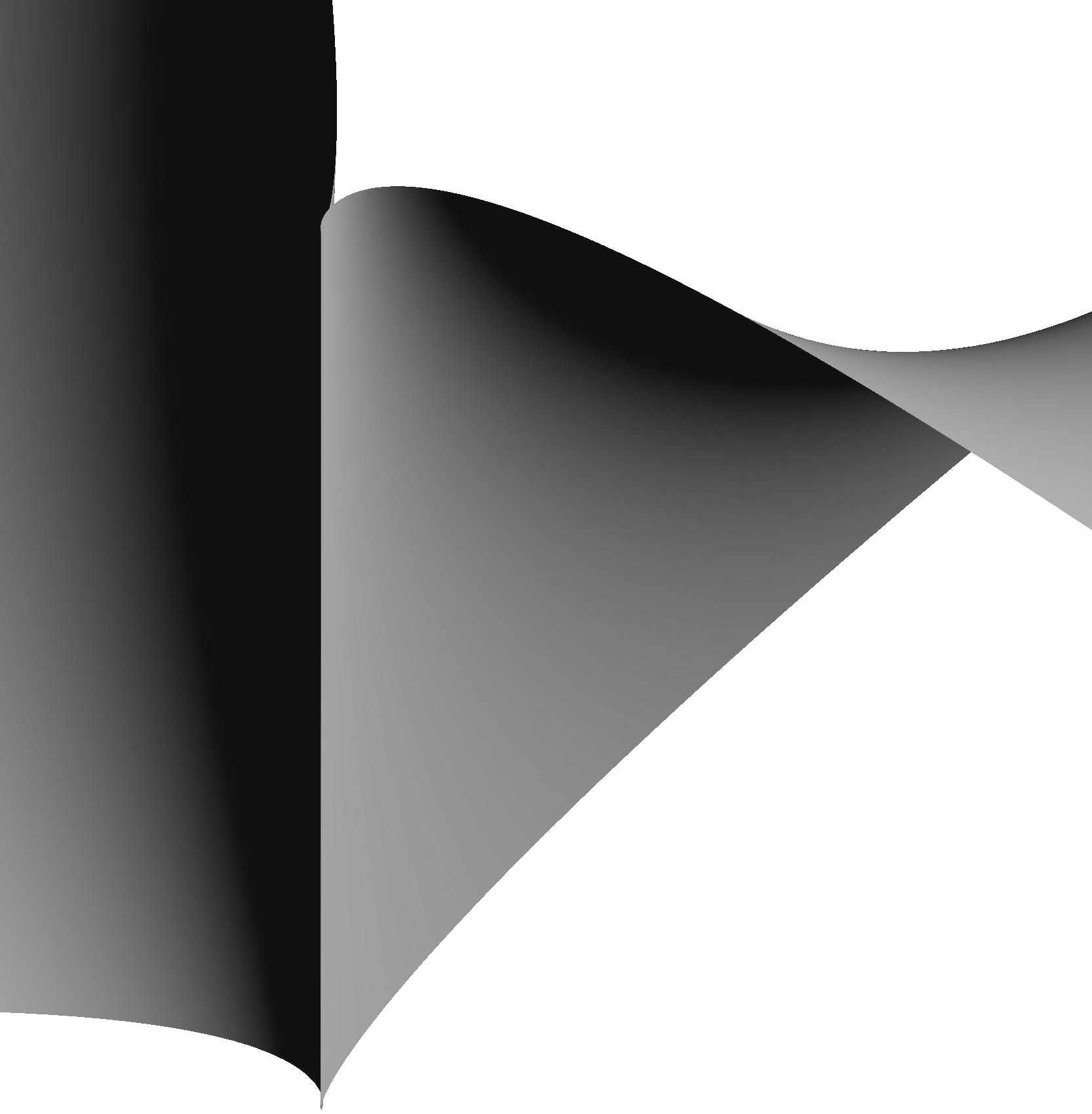
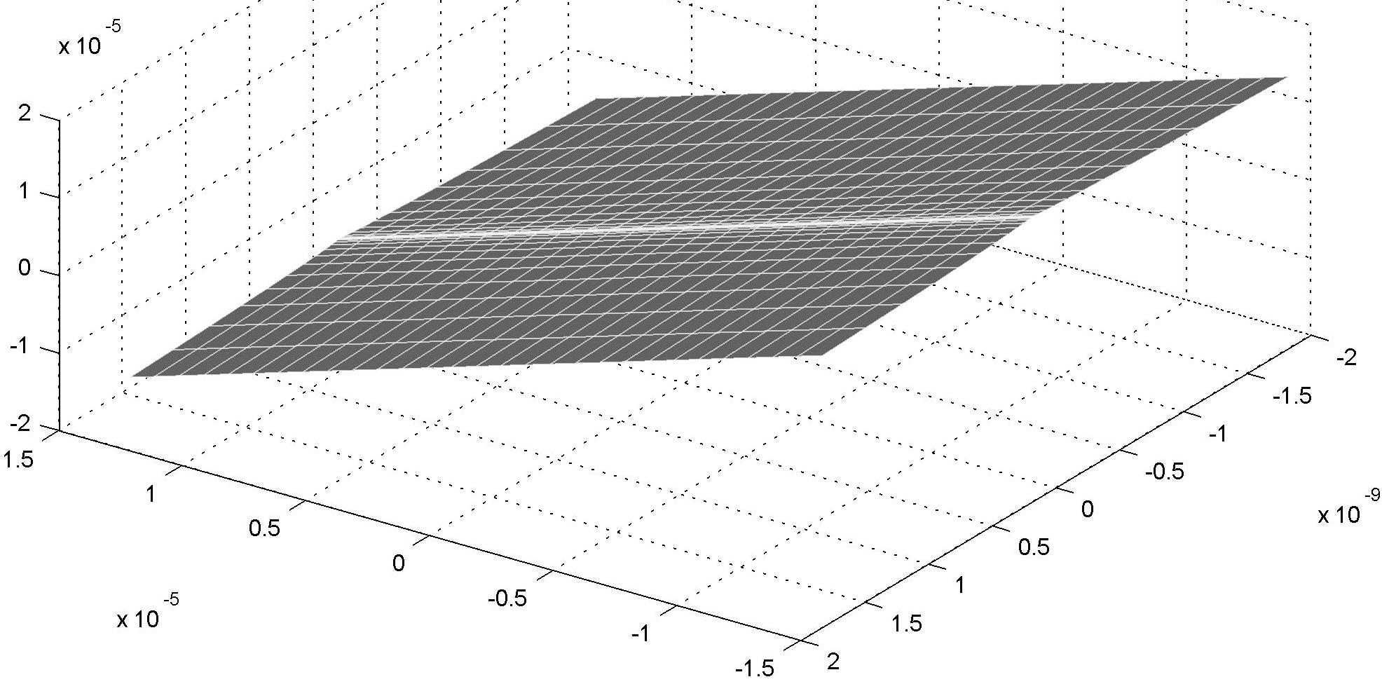
Figure 3. Numerical plots of solutions to the characteristic geometric Cauchy problem. Left: $s(x)=1$, $\delta=\sigma=1$. Right: $s(x)=1$, $\delta(y)=y$, $\sigma(y)=1$.

Finally, to determine the condition that ensures that the values of the map $\hat{\Phi}$ are not constrained to the small cell: as in Theorem 5.2, the surface is obtained from $\tilde{\Phi}=\tilde{X}^{-1}\hat{Y}=\hat{G}_{-}\hat{G}_{+}$, and $\hat{\Phi}=\omega_{1}\tilde{\Phi}$ maps some point into the big cell provided that, at some point, $\textup{d}c_{-1}\neq 0$, where

$$\hat{G}_{-}=O_{\infty}(\lambda^{-2})+\begin{pmatrix}1&b_{-1}\lambda^{-1}\\ c_{-1}\lambda^{-1}&1\end{pmatrix},$$

Evaluating derivatives at $(0,0)$, we find that $\textup{d}c_{-1}(0,0)=\sigma(0,0)$, and so the non-degeneracy condition for the potential is

$$\sigma(0)\neq 0.\\$$

We do not analyze the types of singularities involved here, but two examples of solutions are illustrated in Figure 3, one appearing to be a cuspidal edge and the other appearing to be a singularity of the parameterization, rather than a true geometric singularity.

8. Examples of degenerate singularities

Examples of the way various degenerate geometric Cauchy data impact the resulting construction are illustrated in Figures 4 and 5.

$\begin{array}[]{cc}\includegraphics[height=71.13188pt]{images/degen1E}&\quad\includegraphics[height=71.13188pt]{images/degen3E}\\ s(v)=t(v)=1,\,\,\theta^{\prime}(v)=0.1.&\quad s(v)=3,\,\,t(v)=2,\,\,\theta^{\prime}(v)=0.\end{array}$

Figure 4. "Surfaces" constructed from data which never enters the big cell.

The images in Figure 4 are degenerate along the entire curve $u=0$. They are completely degenerate in the big cell sense, because in one $s=t$ along the whole line, and in the other $\theta^{\prime}=0$ along the whole line. The map $\hat{\Phi}$ never takes values in the big cell, and the map $f$ is just a curve.

$\begin{array}[]{cc}\includegraphics[height=99.58464pt]{images/degen4_2E}&\quad\includegraphics[height=99.58464pt]{images/degen5_2E}\\ s(v)=1,\,\,t(v)=0,\,\,\theta^{\prime}(v)=0.0001&\quad s(v)=1,\,\,t(v)=2,\,\,\theta^{\prime}(v)=0.01v\end{array}$

Figure 5. Surfaces with degenerate singularities.

The first image in Figure 5 is also degenerate along the whole line, because $t(v)=0$, but this time only from the point of view of the theory of frontals. The potential is non-degenerate, but not regular, which results in a degenerate singularity (see Proposition 6.5). The surface folds back over itself along the curve $u=0$, which is the curve along the right hand side of this image.

The last surface is degenerate only at the point $u=v=0$. It has the appearance of a cuspidal cross cap.

References

- [1] A I Bobenko, Surfaces in terms of 2 by 2 matrices. Old and new integrable cases, Harmonic maps and integrable systems, Aspects Math., no. E23, Vieweg, 1994, pp. 83–127.
- [2] D Brander, Singularities of spacelike constant mean curvature surfaces in Lorentz-Minkowski space, Math. Proc. Cambridge Philos. Soc. 150 (2011), 527–556.
- [3] D Brander and J Dorfmeister, Generalized DPW method and an application to isometric immersions of space forms, Math. Z. 262 (2009), 143–172.
- [4] D Brander, W Rossman, and N Schmitt, Holomorphic representation of constant mean curvature surfaces in Minkowski space: Consequences of non-compactness in loop group methods, Adv. Math. 223 (2010), 949–986.
- [5] D Brander and M Svensson, The geometric Cauchy problem for surfaces with Lorentzian harmonic Gauss maps, arXiv:1009.5661 [math.DG].
- [6] J Dorfmeister, J Inoguchi, and M Toda, Weierstrass-type representation of timelike surfaces with constant mean curvature, Contemp. Math. 308 (2002), 77–99, Amer. Math. Soc., Providence, RI.
- [7] J Dorfmeister, F Pedit, and H Wu, Weierstrass type representation of harmonic maps into symmetric spaces, Comm. Anal. Geom. 6 (1998), 633–668.
- [8] J F Dorfmeister, Generalized Weierstraß representations of surfaces, Adv. Stud. Pure Math. (2008), 55–111.
- [9] I Fernandez and F J Lopez, Periodic maximal surfaces in the Lorentz-Minkowski space , Math. Z. 256 (2007), 573–601.
- [10] I Fernandez, F J Lopez, and R Souam, The space of complete embedded maximal surfaces with isolated singularities in the 3-dimensional Lorentz-Minkowski space, Math. Ann. 332 (2005), 605–643.
- [11] S Fujimori, K Saji, M Umehara, and K Yamada, Singularities of maximal surfaces, Math. Z. 259 (2008), 827–848.
- [12] G Ishikawa and Y Machida, Singularities of improper affine spheres and surfaces of constant Gaussian curvature, Internat. J. Math. 17 (2006), 269–293.
- [13] Y W Kim, S-E Koh, H Shin, and S-D Yang, Spacelike maximal surfaces, timelike minimal surfaces, and Björling representation formulae, J. Korean Math. Soc. 48 (2011), 1083–1100.
- [14] Y W Kim and S D Yang, Prescribing singularities of maximal surfaces via a singular Björling representation formula, J. Geom. Phys. 57 (2007), 2167–2177.
- [15] M Kokubu, W Rossman, K Saji, M Umehara, and K Yamada, Singularities of flat fronts in hyperbolic space, Pacific J. Math. 221 (2005), 303–351.
- [16] S Murata and M Umehara, Flat surfaces with singularities in Euclidean 3-space, J. Differential Geom. 82 (2009), 279–316.
- [17] A Pressley and G Segal, Loop groups, Oxford Mathematical Monographs, Clarendon Press, Oxford, 1986.
- [18] K Saji, M Umehara, and K Yamada, The geometry of fronts, Ann. of Math. (2) 169 (2009), 491–529.
- [19] Y Umeda, Constant-mean-curvature surfaces with singularities in Minkowski 3-space, Experiment. Math. 18 (2009), 311–323.
- [20] M Umehara and K Yamada, Maximal surfaces with singularities in Minkowski space, Hokkaido Math. J. 35 (2006), 13–40.