Hawking temperature in the eternal BTZ black hole: an example of Holography in AdS spacetime

We review the relation between AdS spacetime in 1+2 dimensions and the BTZ black hole. Later we show that a ground state in AdS spacetime becomes a thermal state in the BTZ black hole. We show that this is true in the bulk and in the boundary of AdS spacetime. The existence of this thermal state is tantamount to say that the Unruh effect exists in AdS spacetime and becomes the Hawking effect for an eternal BTZ black hole. In order to make this we use the correspondence introduced in Algebraic Holography between algebras of quasi-local observables associated to wedges and double cones regions in the bulk of AdS spacetime and its conformal boundary respectively. Also we give the real scalar quantum field as a concrete heuristic realization of this formalism.

1 Introduction

In recent years there has been great interest in the so-called AdS/CFT correspondence. It seems fair to say that the majority of works on this topic belong to the string theory framework. However, in the context of Quantum Field Theory (QFT), also some approaches to the AdS/CFT correspondence have been proposed. More precisely, in the context of Algebraic Quantum Field Theory (AQFT) there appeared Algebraic Holography (AH) [1]. Algebraic Holography relates a covariant quantum field theory in the bulk and a conformally covariant quantum field theory on the conformal boundary of AdS spacetime. In this sense AH gives an AdS/CFT correspondence too. Also there has appeared the boundary-limit holography [2] where it has been constructed a correspondence between $n$-point functions of a covariant quantum field theory in the bulk and a conformally covariant quantum field theory in the boundary of AdS spacetime. More recently, partly motivated for these works, there appeared Pre-Holography [3], which studied some aspects of the correspondence between field theories in the bulk and in the boundary of AdS spacetime by using the symplectic structure associated to the phase space of the Klein-Gordon operator. When we take into account these works, it is clear that even at the level of QFT there are interesting aspects of the AdS/CFT correspondence which deserve to be studied. Amongst these aspects of the AdS/CFT in QFT which has been studied so far it is, for example, how the global ground state in the bulk of AdS spacetime maps to a state in its boundary [3].

In QFT besides ground states the equilibrium thermal states are outstanding elements in the theory. So, after studying the mapping of a ground state it is very natural to ask how an equilibrium thermal state maps from the bulk to the boundary of AdS spacetime. This issue is more appealing when one knows that models of black holes can be obtained from AdS spacetime. In particular it is known that in three dimensions there exists a solution to the Einstein’s field equations which can be considered as a model of a black hole, the BTZ black hole (BTZbh) [4]. This solution can be obtained directly from the Einstein’s field equations or by making identifications in a proper subset of AdS spacetime [4].

The purpose of this work is to study how a ground state in AdS spacetime in three dimensions is related to an equilibrium thermal state in the BTZbh and how it maps to its boundary. We address this issue by using the abstract setting of Algebraic Holography and by considering a quantum real scalar field. One conclusion we obtain from this investigation is that the Unruh effect takes place in the boundary and in the bulk of AdS spacetime in 1+2 dimensions, and that after a quotient procedure this effect becomes the Hawking effect for the eternal BTZ black hole. This work also will give details of calculations that will be used in the complementary work [5].

In our study the symmetries of AdS spacetime are fundamental. The principal fact is that the group $SO_{0}(2,2)$ acts in AdS spacetime and in its conformal boundary. In AdS spacetime it acts as the isometry group and in its conformal boundary as the global conformal group. This is fundamental in making AH possible. Also, although indirectly, the Tomita-Takesaki and Wichmann-Bisogano theorems play a fundamental rôle. These mathematical aspects are relevant when addressing our problem in the abstract setting. When we give a concrete heuristic example of this formalism we use the procedure given in [2] to obtain a two point function in the boundary of AdS spacetime from a two point function in its bulk.

This work is organized as follows: in section 2 we introduce some aspects of AdS spacetime in 1+2 dimensions relevant for this work. In section 3 we give the generalities of the BTZbh. In section 4 we study the relation of the BTZbh and the boundary of AdS spacetime. In section 5 we define wedge regions in AdS spacetime and show that the exterior of the BTZbh is a wedge regions. Also we proof that the subgroup of AdS group which leaves invariant the exterior of the BTZbh corresponds to the Lorentz boost which leaves invariant the Rindler wedge of the $2$-dimensional Minkowski spacetime at infinity of AdS spacetime. In section 6 we proof that an equilibrium thermal state in AdS spacetime maps to an equilibrium thermal state in the BTZbh. This state is invariant under translations of BTZ time. Also we give as a heuristic realization of this formalism the real quantum scalar field. In appendix A we construct the finite transformations of the global conformal group in two dimensions.

2 AdS spacetime in 1+2 dimensions

In 1+2 dimensions AdS spacetime can be introduced as follows: Let us consider $\mathbb{R}^{4}$ endowed with metric

$$ds^{2}=-du^{2}-dv^{2}+dx^{2}+dy^{2}.$$ (1)

We denote the resulting semi-Euclidian space by $\mathbb{R}^{2,2}$. AdS spacetime in 1+2 dimensions can be identified with the hypersurface in $\mathbb{R}^{2,2}$ defined by

$$-u^{2}-v^{2}+x^{2}+y^{2}=-\ell^{2}$$ (2)

for fixed $\ell$ and with metric induced by the pull back of (1) to (2) under the inclusion map.

At infinity the limit of (2) is [6]

$$-u^{2}-v^{2}+x^{2}+y^{2}=0,$$ (3)

which we call the null cone and denote by $\mathcal{C}^{4}$. The projective cone obtained from the null cone is the compactification of a two dimensional Minkowski spacetime. In this Minkoswski spacetime we can introduce coordinates [7] p. 15

$$\xi^{1}=\frac{u}{v+x}\hskip 28.45274pt\xi^{2}=\frac{y}{v+x}$$ (4)

and a metric $\eta_{\mu\nu}=\textrm{diag}(-1,1)$. These coordinates do not cover all the manifold, points at infinity are left out. Both manifolds, (2) and (3), are invariant under $X\leftrightarrow-X$, hence AdS spacetime modulo this identification has a compactified Minkowski spacetime at infinity. From (3) we see that the topology of $\mathcal{C}^{4}$ is the topology of $\mathbb{S}^{1}\times\mathbb{S}^{1}/{\pm I}$.

The expressions (2) and (3) both are invariant under the orthogonal group $O(2,2)$. In particular they are invariant under its connected component, namely $SO_{0}(2,2)$. However the action of this group has a different meaning when acting on the hypersurfaces defined by these expressions. In the first case it acts as rotations of $\mathbb{R}^{2,2}$ which preserve (2), and we call it AdS group; whereas by preserving (3) it acts on (4) as the global conformal group in $2$-dimensional Minkowski spacetime.

Now let us introduce global and Poincaré charts.

2.1 Global coordinates

Global coordinates $(\lambda,\rho,\theta)$ can be defined by

$$v=\ell\sec\rho\cos\lambda\hskip 28.45274ptu=\ell\sec\rho\sin\lambda$$

$$x=\ell\tan\rho\cos\theta\hskip 28.45274pty=\ell\tan\rho\sin\theta,$$ (5)

where $(\lambda,\rho,\theta)\in[-\pi,\pi)\times[0,\pi/2)\times[-\pi,\pi)$. In these coordinates the metric is

$$ds^{2}=\ell^{2}\sec^{2}\rho\left(-d\lambda^{2}+d\rho^{2}+\sin^{2}\rho d\theta^{2}\right).$$ (6)

From (2.1) we see that $\rho\rightarrow\pi/2$ corresponds to infinity. The metric (6) is not defined on this point, however we can define an usually called unphysical metric as $d\tilde{s}^{2}=\Omega^{2}ds^{2}$ with $\Omega=\frac{1}{\ell}\cos\rho$ and get $d\tilde{s}^{2}=-d\lambda^{2}+d\rho^{2}+\sin^{2}\rho d\theta^{2}$. This metric is well defined for $\rho\in[0,\pi/2]$. When constructing a Penrose diagram for AdS spacetime this is the metric most commonly used [8]. This is the metric of the Einstein universe, but it cover just half of it since $\rho\in[0,\pi/2]$. Using this conformal mapping we can attach a boundary to AdS spacetime. This boundary is given by $\rho=\pi/2$ and its metric is

$$d\tilde{s}^{2}_{b}=-d\lambda^{2}+d\theta^{2}.$$ (7)

The boundary is $\mathbb{S}^{1}\times\mathbb{S}^{1}$ if we make the identification of $-\pi$ and $\pi$ in the domain of $\lambda$ and $\theta$. We can implement $X\leftrightarrow-X$ by antipodal identification in these two circles. In order to avoid close timelike curves it is customary to work with the covering space of AdS spacetime (CAdS), i.e., by letting $\lambda$ to vary on $\mathbb{R}$, and then the boundary of CAdS is an infinite long cylinder $\mathbb{R}\times\mathbb{S}^{1}$. It is again an Einstein universe but in two dimensions.

2.2 Poincaré coordinates

Poincaré coordinates $(T,k,z)$ are given by [9]

$$v=\frac{1}{2z}\left(z^{2}+\ell^{2}+k^{2}-T^{2}\right)\hskip 28.45274ptu=\frac{\ell T}{z}$$

$$x=\frac{1}{2z}\left(\ell^{2}-z^{2}+T^{2}-k^{2}\right)\hskip 28.45274pty=\frac{\ell k}{z}.$$ (8)

In these coordinates the metric is

$$ds^{2}=\frac{\ell^{2}}{z^{2}}\left(-dT^{2}+dk^{2}+dz^{2}\right)$$ (9)

where $(T,k,z)\in(-\infty,\infty)\times(-\infty,\infty)\times(0,\infty)$. In these coordinates, $X\leftrightarrow-X$ can be implemented by $z\leftrightarrow-z$.

3 The BTZ black hole

It is well known there exists a solution to the Einstein’s field equations with negative cosmological constant in three dimensions which can be considered as a model of a black hole [4], better known as the BTZ black hole (BTZbh). The metric of this spacetime is

$$ds^{2}=-f^{2}dt^{2}+f^{-2}dr^{2}+r^{2}(d\phi+N^{\phi}dt)^{2},$$ (10)

where $f^{2}=\left(-M+\frac{r^{2}}{\ell^{2}}+\frac{J^{2}}{4r^{2}}\right)$ and $N^{\phi}=-\frac{J}{2r^{2}}$ with $|J|\leq M\ell$. We call $(t,r,\phi)\in(-\infty,\infty)\times(0,\infty)\times[0,2\pi)$ BTZ coordinates. This metric is asymptotically AdS spacetime since when $r\rightarrow\infty$

$$ds^{2}\sim r^{2}\left(-dt^{2}+d\phi^{2}\right).$$ (11)

Hence the BTZbh is asymptotically $\mathbb{R}\times\mathbb{S}^{1}$, an infinite long cylinder. The horizons are given by

$$r_{\pm}^{2}=\frac{M\ell^{2}}{2}\left(1\pm\left(1-\left(\frac{J}{Ml}\right)^{2}\right)^{1/2}\right)$$ (12)

The BTZ metric can be obtained directly from the Einstein’s field equations by imposing time and axial symmetry [4]. Also, it can be obtained by identifying points in AdS spacetime along the orbits of an appropriate Killing vector of the AdS spacetime [4]. When expressed in BTZ coordinates this Killing vector turns out to be $\partial_{\phi}$.

For the purposes of this work we are interested in the exterior region of the black hole, $r>r_{+}$. This region can be parameterized by [4]

$$u=\sqrt{B(r)}\sinh\tilde{t}\left(t,\phi\right)\hskip 28.45274ptv=\sqrt{A(r)}\cosh\tilde{\phi}\left(t,\phi\right)$$

$$y=\sqrt{B(r)}\cosh\tilde{t}\left(t,\phi\right)\hskip 28.45274ptx=\sqrt{A(r)}\sinh\tilde{\phi}\left(t,\phi\right).$$ (13)

where

$$A(r)=\ell^{2}\left(\frac{r^{2}-r_{-}^{2}}{r_{+}^{2}-r_{-}^{2}}\right),\hskip 28.45274ptB(r)=\ell^{2}\left(\frac{r^{2}-r_{+}^{2}}{r_{+}^{2}-r_{-}^{2}}\right)$$ (14)

and

$$\tilde{t}=\frac{1}{\ell}\left(r_{+}t/\ell-r_{-}\phi\right),\hskip 28.45274pt\tilde{\phi}=\frac{1}{\ell}\left(r_{+}\phi-r_{-}t/\ell\right).$$ (15)

In this parametrization the coordinate $\phi$ must be $2\pi$-periodic in order to obtain the BTZ metric.

An important quantity in our study of thermal states in BTZbh is the surface gravity, $\kappa$. This turns out to be [10] $\kappa=\frac{r_{+}^{2}-r_{-}^{2}}{\ell^{2}r_{+}}$.

For further reference we give in figure 1 the Penrose diagram for the non-rotating BTZbh.

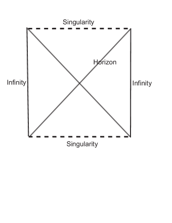
Figure 1: Penrose diagram for the non-rotating BTZ black hole.

4 The BTZ black hole and its relation to the boundary of AdS spacetime

We mentioned before that the BTZbh can be obtained by a quotient procedure from AdS spacetime. This quotient is made by a discrete subgroup of $SO_{0}(2,2)$. Because we want the resulting spacetime not to have closed timelike curves, it is required the Killing vector which generates this subgroup to be spacelike. This criterion turns out to be not just necessary but also sufficient [4]. First let us restrict ourselves to the non-rotating case. In this case, when expressed in embedding coordinates this generator turns out to be

$$\partial_{\phi}=\frac{r_{+}}{\ell}\left(x\partial_{v}+v\partial_{x}\right).$$ (16)

We are interested in studying quantum field theory in the boundary of AdS spacetime and consequently of the BTZbh. So it is useful to find out which regions of the boundary of AdS spacetime correspond to the covering space of the BTZbh. Because the maximally extended BTZbh have two exterior regions analogously to Schwarzschild spacetime, there will be two regions in the boundary which cover the maximally extended BTZbh. If we want to know explicitly these two regions, we can express $\partial_{\phi}$ in global coordinates, take the limit $\rho\rightarrow\pi/2$, and impose on it the condition of being spacelike in the metric (7).

Using (2.1) and (16), in global coordinates

$$\frac{\ell}{r_{+}}\partial_{\phi}=-\sin\lambda\sin\rho\cos\theta\partial_{\lambda}+\cos\lambda\cos\rho\cos\theta\partial_{\rho}-\frac{\cos\lambda\sin\theta}{\sin\rho}\partial_{\theta}.$$ (17)

On the boundary $J_{\phi}\equiv\frac{\ell}{r_{+}}\partial_{\phi}|_{\rho=\pi/2}=-\sin\lambda\cos\theta\partial_{\lambda}-\cos\lambda\sin\theta\partial_{\theta}$. Its norm is given by $||J_{\phi}||^{2}=-\sin^{2}\lambda\cos^{2}\theta+\cos^{2}\lambda\sin^{2}\theta=-\sin u\sin v$, where we have introduced null coordinates $u=\lambda-\theta$ and $v=\lambda+\theta$. Clearly this vector can be timelike, spacelike or null. The regions where it is null are given by $u,v=n\pi$ with $n=0,\pm 1,\pm 2...$ Hence the covering space of the exterior of the BTZbh is the region inside the lines defined by,

$$u=\pi,0,-\pi\hskip 28.45274ptv=\pi,0,-\pi,$$ (18)

see figure 2.

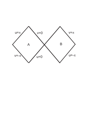
Figure 2: This figure represents the covering space of the BTZbh in the boundary of AdS spacetime in 1+2 dimensions.

This figure has been given in [11] and [12] too.

On the boundary the BTZ coordinates are $(t,\phi)$. We have found already the generator of translations in $\phi$, let us see what the translations in time is. In embedding coordinates

$$\partial_{t}=\frac{r_{+}}{\ell^{2}}\left(y\partial_{u}+u\partial_{y}\right).$$ (19)

Using (2.1) and (19), in global coordinates

$$\frac{\ell^{2}}{r_{+}}\partial_{t}=\sin\lambda\cos\rho\sin\theta\partial_{\rho}+\cos\lambda\sin\rho\sin\theta\partial_{\lambda}+\frac{\sin\lambda\cos\theta}{\sin\rho}\partial_{\theta}.$$ (20)

On the boundary $J_{t}\equiv\frac{\ell^{2}}{r_{+}}\partial_{t}|_{\rho=\pi/2}=\cos\lambda\sin\theta\partial_{\lambda}+\sin\lambda\cos\theta\partial_{\theta}$. The norm of $J_{t}$ is given by $||J_{t}||^{2}=-\cos^{2}\lambda\sin^{2}\theta+\sin^{2}\lambda\cos^{2}\theta=\sin u\sin v$. Clearly ${J_{t}}^{\mu}{J_{\phi}}_{\mu}=0$ and when $J_{\phi}$ is spacelike $J_{t}$ is timelike and viceversa.

Now let us see what the region of the boundary of CAdS covered by the Poincaré chart is. Here we are going to consider just one fundamental region of CAdS, $\lambda\in[-\pi,\pi)$. From (2.1) and (2.2) it follows that

$$\cos\lambda=\frac{z^{2}+\ell^{2}+k^{2}-T^{2}}{\sqrt{\left(z^{2}+\ell^{2}+k^{2}-T^{2}\right)^{2}+\left(2\ell T\right)^{2}}}$$ (21)

and

$$\cos\theta=-\frac{z^{2}-\ell^{2}+k^{2}-T^{2}}{\sqrt{\left(z^{2}+\ell^{2}+k^{2}-T^{2}\right)^{2}+\left(2\ell T\right)^{2}-\left(2\ell z\right)^{2}}}.$$ (22)

By following the analysis in [9] it can be shown that the equality $\cos\lambda=-\cos\theta$ can be satisfied on the surface $\rho=\pi/2$ and it corresponds to, let us say, the boundary of one Poincaré chart in the boundary, see figure 3. We see that the covering region of the maximally extended BTZbh is half of the Poincaré chart. Let us see what the relation between BTZ coordinates and Poincaré coordinates is.

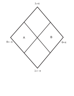
Figure 3: This figure shows how the covering space of BTZ on the boundary is related to the Poincaré chart. The big diamond is the Poincaré chart whereas the covering space of BTZ is the A and B small diamonds.

From (2.2) and (3) it follows that in the boundary

$$T=\ell e^{-\ell\kappa\phi}\sinh\kappa t\hskip 28.45274ptk=\ell e^{-\ell\kappa\phi}\cosh\kappa t.$$ (23)

From (23) we see that the relation between BTZ coordinates and Poincaré coordinates is analogous to the relation between Rindler and Minkowski coordinates [13]. This fact suggests that some kind of Unruh effect is taking place in the boundary of the CAdS spacetime. In the next sections we shall show this is indeed the case.

The vector fields of $\partial_{t}$ and $\partial_{\phi}$ for the non-rotating case are given in figure 4.

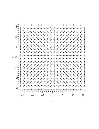
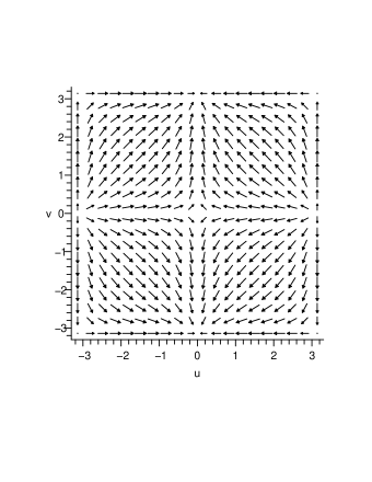
Figure 4: These figures show the vector fields $\partial_{\phi}$ and $\partial_{t}$ respectively for the nonrotating BTZ black hole. These figures were made with Maple 10.

5 Wedge regions in AdS spacetime

In the context of Algebraic Holography [1] wedge regions in AdS spacetime play a prominent rôle. In this section we will show that the exterior of the BTZbh is a wedge region.

Following [1] we define a wedge region in AdS spacetime as follows. Let us take two light-like vectors ($e,f$) in the embedding space $\mathbb{R}^{2,2}$ such that $e\cdot f>0$, then a wedge region in AdS spacetime is defined by

$$\widetilde{W}(e,f)=\{X\in\mathbb{R}^{2+2}:X^{2}=-\ell^{2},e\cdot X<0,f\cdot X<0\}.$$ (24)

This region has two connected components. One where the resulting vector by acting on the tangent vector at the point $X\in\widetilde{W}(e,f)$ with the boost in the $e$-$f$ plane is future directed and other where it is past directed. This is a consequence of the fact that the vector $\delta_{e,f}X=(f\cdot X)e-(e\cdot X)f$ is time-like, $(\delta_{e,f}X)^{2}=-2(e\cdot f)(e\cdot X)(f\cdot X)<0$. The wedges regions are defined in [1] as these regions module the identification $X\leftrightarrow-X$. Hence in order to check that a region in AdS spacetime is a wedge region we just have to verify that it has these properties. Let us do this for the exterior of the BTZbh.

5.1 The exterior of the BTZ black hole is a wedge region

Let us take $e=(1,0,0,-1)$ and $f=(-1,0,0,-1)$. These light-like vectors satisfy $e\cdot f>0$. By using the parametrization (3)-(15) we get

$$e\cdot X=-\sqrt{B(r)}\left(\sinh\tilde{t}+\cosh\tilde{t}\right)<0$$ (25)

and

$$f\cdot X=\sqrt{B(r)}\left(\sinh\tilde{t}-\cosh\tilde{t}\right)<0.$$ (26)

Hence the exterior of the rotating BTZ black hole is a wedge region. It is also true for the non-rotating case. As explained in [1] this wedge intersects the boundary in a double cone. In the previous section we have found this double cone explicitly. These regions are preserved by the action of the subgroup generated by the Killing vector $\partial_{t}$. This group acts on the wedge as a subgroup of the AdS group and as subgroup of the conformal group on the boundary.

5.2 The exterior of BTZ black hole and the Rindler wedge in Minkowski spacetime

We have found that the exterior of BTZ black hole is invariant under the one-parameter subgroup of the AdS group generated by $\partial_{t}$. Let us calculate explicitly this one-parameter subgroup. The generator of this subgroup is given by (19), hence a matrix representation of it on the vector space $\mathbb{R}^{2,2}$ is given by

$$\partial_{t}=\kappa\left(\begin{array}[]{cccc}0&0&0&1\\ 0&0&0&0\\ 0&0&0&0\\ 1&0&0&0\end{array}\right).$$ (27)

The matrix (27) is an element of the Lie algebra of $SO_{0}(2,2)$ and the one-parameter subgroup generated by it is given by

$$\Lambda(t)=e^{t\partial_{t}}=\left(\begin{array}[]{cccc}\cosh\kappa t&0&0&\sinh\kappa t\\ 0&1&0&0\\ 0&0&1&0\\ \sinh\kappa t&0&0&\cosh\kappa t\end{array}\right).$$ (28)

This one-parameter group acts on the vector space $\mathbb{R}^{2,2}$ leaving the exterior of the BTZbh invariant.

As we said in section 2, AdS spacetime has a compactified Minkowski spacetime at infinity. Also we know that $SO_{0}(2,2)$ acts as the conformal group on this Minkowski spacetime [7]. Let us see to which element of the conformal group in two dimensions the element (28) corresponds.

Remembering the definition of the coordinates of Minkowski spacetime at infinity we have

$$\xi^{1}=\frac{u}{v+x}\hskip 28.45274pt\xi^{2}=\frac{y}{v+x}.$$ (29)

If now we let $\Lambda(t)$ to act on $X^{T}=(u,v,x,y)$ we obtain

$$\Lambda(t)x=\left(\begin{array}[]{c}u\cosh\kappa t+y\sinh\kappa t\\ v\\ x\\ u\sinh\kappa t+y\cosh\kappa t\end{array}\right)=\left(\begin{array}[]{c}u^{\prime}\\ v^{\prime}\\ x^{\prime}\\ y^{\prime}\end{array}\right).$$ (30)

This transformation on the null cone, $\mathcal{C}^{4}$, induces a transformation on $\xi^{1}$ and $\xi^{2}$.

$$\xi^{1}\rightarrow\xi^{\prime 1}=\frac{u^{\prime}}{v^{\prime}+x^{\prime}}\hskip 28.45274pt\xi^{2}\rightarrow\xi^{\prime 2}=\frac{y^{\prime}}{v^{\prime}+x^{\prime}}.$$ (31)

From (30) and (29) it follows that

$$\xi^{\prime 1}=\xi^{1}\cosh\kappa t+\xi^{2}\sinh\kappa t\hskip 28.45274pt\xi^{\prime 2}=\xi^{1}\sinh\kappa t+\xi^{2}\cosh\kappa t.$$ (32)

Then the subgroup of the AdS group generated by $\partial_{t}$ corresponds to a Lorentz boost in the two dimensional Minkowski spacetime. From this we can see that the Rindler wedge in this two dimensional Minkowski spacetime is invariant under the action of the subgroup of the global conformal group corresponding to the subgroup of the AdS group generated by $\partial_{t}$. The Rindler wedge just mentioned is the double cone which results from the intersection of the wedge corresponding to the exterior of the BTZ black hole with the boundary.

The correspondence between the others one-parameter subgroups can be found analogously. For example let us analyze the subgroup generated by $\partial_{\phi}$.

The matrix representation of this generator on the vector space $\mathbb{R}^{2,2}$ is given by

$$\partial_{\phi}=\kappa\ell\left(\begin{array}[]{cccc}0&0&0&0\\ 0&0&1&0\\ 0&1&0&0\\ 0&0&0&0\end{array}\right).$$ (33)

Hence the finite transformation is given by

$$\Lambda(\phi)=e^{\phi\partial_{\phi}}=\left(\begin{array}[]{cccc}1&0&0&0\\ 0&\cosh\kappa\ell\phi&\sinh\kappa\ell\phi&0\\ 0&\sinh\kappa\ell\phi&\cosh\kappa\ell\phi&0\\ 0&0&0&1\end{array}\right).$$ (34)

If we let this transformation to act on $X^{T}=(u,v,x,y)$ we obtain

$$\Lambda(\phi)x=\left(\begin{array}[]{c}u\\ v\cosh\kappa\ell\phi+x\sinh\kappa\ell\phi\\ v\sinh\kappa\ell\phi+x\cosh\kappa\ell\phi\\ y\end{array}\right)=\left(\begin{array}[]{c}u^{\prime}\\ v^{\prime}\\ x^{\prime}\\ y^{\prime}\end{array}\right).$$ (35)

This transformation induces a transformation on $\xi^{1}$ and $\xi^{2}$ given by

$$\xi^{\prime 1}=e^{-\kappa\ell\phi}\xi^{1}\hskip 28.45274pt\xi^{\prime 2}=e^{-\kappa\ell\phi}\xi^{1}.$$ (36)

Then the subgroup of AdS group generated by $\partial_{\phi}$ corresponds to the dilation group on the two dimensional Minkowski spacetime.

6 Thermal state in AdS spacetime and in the BTZ black hole

In this section we show that there exists an equilibrium thermal state in AdS spacetime in 1+2 dimensions and discuss its relation to an equilibrium thermal state in the BTZbh.

In the previous section we showed that the exterior of the BTZbh is a wedge region. Now, also the Poincaré chart is likely to be a wedge region. If so we can associate a net of algebras to these regions. This can be done, for example, by adapting the formalism introduced in [15] to the present case. Due to the invariance of these wedges regions under the action of the subgroups generated by $\partial_{T}$ and $\partial_{t}$ we have

$$\omega(\alpha_{T}a)=\omega(a)\hskip 28.45274pta\in A(W_{T})$$ (37)

and

$$\omega(\alpha_{t}a)=\omega(a)\hskip 28.45274pta\in A(W_{t}),$$ (38)

where $W_{T}$ and $W_{t}$ are the wedge regions associated to the Poincaré chart and the exterior of the BTZbh respectively, and $A$ is a von Neumann algebra. The symbol $\omega$ denote a state on these algebras, below we explain more about this state. The symbols $\alpha_{T}$ and $\alpha_{t}$ denote the automorphisms of the algebras associated to $W_{T}$ and $W_{t}$ respectively. We assume that these automorphisms satisfy

$$\alpha_{T}A(W_{T})=A(\Lambda(T)W_{T})$$ (39)

and

$$\alpha_{t}A(W_{t})=A(\Lambda(t)W_{t})$$ (40)

where $\Lambda(T)$ and $\Lambda(t)$ are the transformations which leave invariant $W_{T}$ and $W_{t}$ respectively. The last four expressions deserve some comments. The existence of $\Lambda(T)$ and $\Lambda(t)$ is a consequence of the existence of the Killing vectors $\partial_{T}$ and $\partial_{t}$, which is a geometrical property of AdS spacetime. The equations (39) and (40) are part of the assumptions about the structure of the algebras. The equations (37) and (38) are a consequence of analogous expressions in the boundary assuming AH. Hence once we are in AdS spacetime and its geometry and we postulate the algebraic structure on its boundary these four equations should be valid. Now let us make some comments about the state $\omega$. As we have said the last four equations have a bulk and boundary counterpart. In the boundary we have a Minkowski spacetime whereas in the bulk a spacetime with constant curvature. If we want to make quantum field theory on both and both should be equivalent there should be no preference for one of these two perspectives a priori. However if we take into account that Quantum Field Theory in Minkowski spacetime has a well establish theory it seems that we should go from the boundary to the bulk, because in this way we can use all the formalism at hand for QFT in Minkowski spacetime and try to apply it to the bulk of AdS spacetime. It could be possible that some tools for Minkowski spacetime do not apply to AdS spacetime however we will notice this if we get a contradiction or an unphysical result. By taking this philosophy it seems that we should take the ground state on the boundary defined with respect to $\partial_{T}$ as the vacuum of the theory on the boundary. If we do this then in the bulk $\omega$ will be our vacuum, i.e., if we make the GNS construction [7] of this state then the unitary operator associated with translations in $T$ has a self-adjoint generator operator, $H_{T}$, with spectrum $[0,\infty]$. This hamiltonian satisfies

$$H_{T}|\Psi_{\omega}\rangle=0,$$ (41)

where $|\Psi_{\omega}\rangle$ is the cyclic vector associated with $\omega$ through the GNS construction. Also we have assumed the unitary operator implementing translation in $T$ is strongly continuos with respect to $T$. Hence in this case the Von Neumann’s theorem [16] assures the existence of $H_{T}$.

As was proven in [1], once we have set up this scenario we can apply the well-known theorems of Takesaki-Tomita and Bisognano-Wichmann to the theory on the boundary. From this it follows that the vacuum in the boundary becomes an equilibrium thermal state with respect to $t$ when restricted to the double cone associated with the exterior region of the BTZbh. This is on the boundary. Now, by applying Algebraic Holography we obtain that the same is valid in the bulk, so $\omega$ in the bulk is also an equilibrium equilibrium thermal state with respect to $t$ when restricted to the exterior of the BTZbh. Put in other way, it satisfies the KMS condition with respect to $t$. Let us find what the temperature of this state is.

From (30) we can see that the parameter of the boost is $t^{\prime}=\kappa t$ with $\kappa=\frac{r_{+}}{\ell^{2}}$. Using the theorem 4.1.1 (Bisognano-Wichmann theorem) in [7] we have that the parameter of the modular group which appears in the Tomita-Takesaki theorem is given by

$$\tau=-\frac{t^{\prime}}{2\pi}=-\frac{\kappa}{2\pi}t.$$ (42)

Using the theorem 2.1.1 (Tomita-Takesaki theorem) in [7] it is possible to proof the state invariant under the modular group satisfies the KMS condition with $\beta=-1=\frac{1}{\textsf{T}}$, see [7] p. 218

$$\omega\left(\left(\alpha_{\tau}A\right)B\right)=\omega\left(B\left(\alpha_{\tau-i}A\right)\right).$$ (43)

Hence from (42) it follows the temperature of the thermal state with respect to $t$ is

$$\textsf{T}=\frac{\kappa}{2\pi}.$$ (44)

This is the so-called temperature of the black hole. The local temperature measure by an observer at constant radius $r$ is

$$\textsf{T}(r)=\frac{1}{(-g_{00})^{1/2}}\frac{\kappa}{2\pi}.$$ (45)

This is because the proper time of this observer, $\lambda$, and the time $t$ are related as $\lambda=(-g_{00})^{1/2}t$.

So far we have shown that $\omega$ satisfies the KMS condition on the covering space of one exterior of the BTZbh, however the exterior of the BTZbh is obtained after making $\phi$ 2$\pi$-periodic. This periodicity introduces new features because we have a non simply connected spacetime, a cylinder, instead of a simply connected spacetime, a plane. We shall assume that there is a way to construct the thermal state on the cylinder from one on the plane algebraically. Let us call the state on the covering space of one exterior region of the BTZbh $\omega_{AdS}$ and on the exterior region of the BTZbh $\omega_{BTZ}$.

The state $\omega_{BTZ}$ is defined in $\mathbb{R}^{1}\times\mathbb{S}^{1}$ which is one exterior region of the BTZ black hole whereas $\omega_{AdS}$ is defined on $\mathbb{R}^{1}\times\mathbb{R}^{1}$ which is the covering space of one exterior region of the BTZ black hole. Put in this way, the state $\omega_{BTZ}$ is a thermal state on a black hole, i.e., the Hawking effect for an eternal black hole takes place and corresponds to the Unruh effect on AdS after making $\phi$ 2$\pi$-periodic. Put in this form we can say that the Hawking effect in the eternal BTZbh has its origin in the Unruh effect in the boundary of AdS spacetime and in the topological relation between $\mathbb{R}^{1}\times\mathbb{R}^{1}$ and $\mathbb{R}^{1}\times\mathbb{S}^{1}$.

In the rotating case there is a tiny modification in the analysis. From the form of the parametrization of the exterior of BTZ black hole (3) we see that in the rotating case the subgroup of the AdS group which leaves invariant the wedge $W$ is generated by $\partial_{\tilde{t}}$. Following the analysis of the previous section, now the parameter of the modular group which appears in Tomita-Takesaki theorem is related to the time $\tilde{t}$ as

$$\tau=-\frac{\tilde{t}}{2\pi}.$$ (46)

Hence the state is thermal with respect to $\tilde{t}$ at temperature $\textsf{T}=\frac{1}{2\pi}$. Put in this form, because the state $\omega$ satisfies

$$\omega\left(\left(\alpha_{\tilde{t}-2\pi}A\right)B\right)=\omega\left(B\left(\alpha_{\tilde{t}}A\right)\right),$$ (47)

then there is a periodicity of the state in $t$ and $\phi$ given by

$$(t,\phi)\rightarrow(t-i\beta,\phi+i\Omega_{H}\beta)\hskip 28.45274pt\beta=\frac{1}{\textsf{T}}=\frac{2\pi}{\kappa}.$$ (48)

where $\beta=\frac{2\pi}{\kappa}$. Hence again the black hole is hot at temperature $\textsf{T}=\frac{\kappa}{2\pi}$.

6.1 Thermal state for a real quantum scalar field

In this section we show how an equilibrium thermal state in the bulk of AdS spacetime maps to an equilibrium thermal state on its boundary for a real quantum scalar field.

The equation the field satisfies is

$$\left(\nabla_{\mu}\nabla^{\mu}-\xi R-m^{2}\right)\phi=0,$$ (49)

where $\xi$ is a coupling constant, $R$ is the Ricci scalar and $m$ can be considered as the mass of the field. For the metric of AdS spacetime, $R=6\Lambda=-\frac{6}{\ell^{2}}$. Hence the last equation can be written as

$$\left(\nabla_{\mu}\nabla^{\mu}-\widetilde{m}^{2}\right)\phi=0,$$ (50)

where $\widetilde{m}^{2}=m^{2}-\frac{6\xi}{\ell^{2}}$. For our purposes it is convenient to use Poincaré coordinates. In these coordinates $g=-\frac{\ell^{6}}{z^{6}}$. Because $\partial_{T}$ and $\partial_{k}$ are Killing vectors we propose the ansatz $\phi(T,k,z)\propto e^{-i\omega T}e^{ink}f_{\omega n}(z)$.

The normalized modes turns out to be [18]

$$F_{na}(T,k,z)=\left(\frac{a}{4\ell\pi\omega}\right)^{\frac{1}{2}}e^{-i\omega T}e^{ink}zJ_{p}(az).$$

It follows that the two point function is [18]

$$F(\Delta T,\Delta k;z,z^{\prime}) = \frac{(zz^{\prime})^{1+p}}{2\ell\pi}\lim_{\epsilon\rightarrow 0_{+}}\Bigg{\{}$$

$$\frac{F_{4}\left(\alpha,\alpha;\alpha,\alpha;-\frac{z^{2}}{(\Delta k)^{2}-(\Delta T+i\epsilon)^{2}},-\frac{z^{\prime 2}}{(\Delta k)^{2}-(\Delta T+i\epsilon)^{2}}\right)}{((\Delta k)^{2}-(\Delta T+i\epsilon)^{2})^{1+p}}\Bigg{\}}$$

where $\alpha=1+p$, $p^{2}=1+\ell^{2}\widetilde{m}^{2}$ and $F_{4}$ is a Hypergeometric function of two variables. Following [2] we now make $z=z^{\prime}$ and multiply (6.1) by $z^{-2(1+p)}$ and take the limit $z\rightarrow 0$ we obtain

$$F_{b}(\Delta T,\Delta k) \equiv \lim_{z\rightarrow 0}z^{-2(1+p)}F(\Delta T,\Delta k;z,z)$$ (52)

$$= \frac{1}{2\ell\pi}\lim_{\epsilon\rightarrow 0_{+}}\frac{1}{((\Delta k)^{2}-(\Delta T+i\epsilon)^{2})^{1+p}}.$$

Now let us analyze what happens when we restrict (52) to the exterior of BTZ black hole. By using (23) we get

$$F_{b}(\Delta t,\Delta\phi^{\prime})=\frac{1}{2\ell\pi}\frac{(2\ell^{2}e^{-\kappa(\phi_{1}^{\prime}+\phi_{2}^{\prime})})^{-1-p}}{(\cosh\kappa\Delta\phi^{\prime}-\cosh\kappa\Delta t-i\epsilon)^{1+p}},$$ (53)

where $\phi^{\prime}=\ell\phi$.

From (53) it follows that

$$F_{b}(-\Delta t,\Delta\phi^{\prime})=F_{b}(\Delta t-i\beta,\Delta\phi^{\prime})$$ (54)

where $\beta=\frac{1}{\textsf{T}}=\frac{2\pi}{\kappa}$. From (54) it follows that the restricted two point function to the exterior of the BTZbh in the boundary satisfies the KMS condition [19]. Hence (6.1) is a thermal state at temperature $\textsf{T}=\frac{\kappa}{2\pi}$ when restricted to the exterior of the BTZbh. From (6.1) we see that the thermal property does not change when we take the limit $z\rightarrow 0$, since $z=\ell e^{-\kappa\phi^{\prime}}\frac{r_{+}}{r}$, hence we can say the thermal state in the bulk of AdS maps to a thermal state on its boundary, and this state is given by (53).

The Jacobian of (23) is

$$\left|\frac{\partial(T,k)}{\partial(t,\phi^{\prime})}\right|=\ell^{2}\kappa^{2}e^{-2\kappa\phi^{\prime}}.$$ (55)

If we consider (23) as a conformal transformation then from (55) and the relationship between two conformal metrics

$$g_{\mu\nu}^{\prime}(x^{\prime})=\Omega^{2}(x)g_{\mu\nu}(x)$$ (56)

it follows that in the present case

$$\Omega(\phi^{\prime})=\frac{1}{\ell\kappa e^{-\kappa\phi^{\prime}}}.$$ (57)

If we want to consider $F_{b}$ as a correlation function for a conformal field theory in the boundary of AdS spacetime and take into account two correlation function in a conformal field theory are related by [20] p. 104

$$\Omega(x_{1}^{\prime})^{-\Delta_{1}}\Omega(x_{2}^{\prime})^{-\Delta_{2}}\langle\phi_{1}(x_{1}^{\prime})\phi_{2}(x_{2}^{\prime}))\rangle=\langle\phi_{1}(x_{1})\phi_{2}(x_{2})\rangle,$$ (58)

where $\Delta_{1}$ and $\Delta_{2}$ are the scaling dimension of the field $\phi_{1}$ and $\phi_{2}$ respectively, then from the equality

$$\frac{1}{2\pi}\frac{\Omega(\phi_{1}^{\prime})^{-1-p}\Omega(\phi_{2}^{\prime})^{-1-p}}{((\Delta k)^{2}-(\Delta T+i\epsilon)^{2})^{1+p}}=\frac{2^{-1-p}}{2\pi}\frac{\kappa^{2(1+p)}}{(\cosh\kappa\Delta\phi^{\prime}-\cosh\kappa\Delta t-i\epsilon)^{1+p}}$$

we finally have

$$F_{b}(\Delta t,\Delta\phi^{\prime})\simeq\frac{1}{2\ell\pi 2^{(1+p)}}\frac{\kappa^{2(1+p)}}{(\cosh\kappa\Delta\phi^{\prime}-\cosh\kappa\Delta t-i\epsilon)^{(1+p)}}.$$ (59)

According to standard conformal field theory [20] this correlation function would correspond to a field with scaling dimension $\Delta=1+p$.

From (59) we can obtain the two correlation functions on the exterior of BTZ black hole and its covering space respectively by using the image method. Let us explain briefly this method. The image sum method relates the two point function in a multiple connected and the two point function in a simply connected spacetime, see [21] or [22]. In this case we could apply the formula

$$F^{\prime}_{b}(\Delta t,\Delta\phi)=\sum_{n\in\mathbb{Z}}e^{2\pi in\alpha}F_{b}(\Delta t,\Delta\phi+2\pi n),$$ (60)

where $F^{\prime}_{b}(\Delta t,\Delta\phi)$ is the two point function in the covering space of the exterior of BTZ black hole and $\alpha$ a parameter which is $0$ for untwisted and $\frac{1}{2}$ for twisted fields. In this work we are interested in untwisted fields, so we take $\alpha=0$. Applying this method to (59) we obtain

$$F^{\prime}_{b}(\Delta t,\Delta\phi) \equiv \sum_{n\in\mathbb{Z}}\frac{1}{2\ell\pi 2^{(1+p)}}\times$$ (61)

$$\times \frac{\kappa^{2(1+p)}}{(\cosh\kappa\ell(\Delta\phi+2\pi n)-\cosh\kappa\Delta t-i\epsilon)^{(1+p)}}.$$

This correlation function would correspond to fields defined on the same covering space of one exterior region of BTZ black hole. However BTZ black hole has two exterior regions analogously to Schwarzschild black hole. The parametrization of the other exterior region is given by changing the sign in (23). Hence in this case the correlation function is

$$F^{\prime}_{b}(\Delta t,\Delta\phi) \equiv \sum_{n\in\mathbb{Z}}\frac{1}{2\ell\pi 2^{(1+p)}}\times$$ (62)

$$\times \frac{\kappa^{2(1+p)}}{(\cosh\kappa\ell(\Delta\phi+2\pi n)+\cosh\kappa\Delta t+i\epsilon)^{(1+p)}}.$$

From the previous analysis is clear that on the boundary we have a thermal state when we restrict the state defined on the Poincaré chart to the covering space of one exterior region of the BTZbh. Also because we have to make $\phi$ $2\pi$-periodic then this covering space is a cylinder with spatial cross section. Now a massless field theory on a cylinder is equivalent to a two dimensional conformal field theory [20], hence we can say that on the boundary of AdS we have two conformal theories related in such way that when we restrict a vacuum state to one of them it becomes a thermal state. We point out that the expressions (61) and (62) have been given in [23] and according to it they have been obtained in [24]. In [24] it was used the proposal given in [6] for the AdS/CFT correspondence. However we have just obtained them by using AdS/CFT in QFT which uses both Algebraic Holography and the boundary-limit Holography. This last procedure can be considered as alternative to the procedure used by Keski-Vakkuri.

So far in this section we have considered the non rotating BTZ black hole. However similar considerations apply to the rotating case. In the rotating case the relation between Poincaré and BTZ coordinates is

$$T=\pm\ell\left(\frac{r^{2}-r_{+}^{2}}{r^{2}-r_{-}}\right)^{1/2}e^{-\tilde{\phi}}\sinh\tilde{t}\hskip 28.45274ptk=\pm\ell\left(\frac{r^{2}-r_{+}^{2}}{r^{2}-r_{-}}\right)^{1/2}e^{-\tilde{\phi}}\cosh\tilde{t},$$ (63)

where $\tilde{t}$ and $\tilde{\phi}$ are defined in (15). Hence in the limit $r\rightarrow\infty$

$$T=\pm\ell e^{-\tilde{\phi}}\sinh\tilde{t}\hskip 28.45274ptk=\pm\ell e^{-\tilde{\phi}}\cosh\tilde{t}.$$ (64)

The sign $+$ corresponds to one exterior of BTZ black hole and the sign $-$ to the other. Following the analysis for the non-rotating case we have

$$F_{b}(-\Delta\tilde{t},\Delta\tilde{\phi})=F_{b}(\Delta\tilde{t}-i2\pi,\Delta\tilde{\phi})$$ (65)

if

$$(t,\phi)\rightarrow(t-i\beta,\phi+i\beta\Omega_{H})$$ (66)

where $\beta=\frac{1}{\textsl{T}}$ and $\Omega_{H}$ is the angular velocity of the horizon.

7 Summary and open questions

In this work, apart from reviewing the relationship between AdS spacetime and the BTZ black hole, we studied how a ground state (the Poincaré vacuum) in AdS spacetime in 1+2 dimensions becomes a thermal state in the BTZ black hole. We address this issue in the abstract setting of Algebraic Holography and in a concrete example of the quantum real scalar field. We found both approaches consistent and we can say that the Unruh effect in AdS spacetime becomes the Hawking effect for the eternal BTZ black hole. In doing this we obtained that the thermal state in the BTZ black hole maps to its boundary. This state coincides with the state obtained in [24] by a rather different methods based on the proposal [6] for the AdS/CFT correspondence. So, a natural question we can ask ourselves is to find out the reason of this coincidence. Is it accidental? Or, what is the reason in this case the two approaches [2] and [6] give the same result? We leave these questions open for now and hope to solve them in future work.

Acknowledgments: I thank my supervisor, Dr. Bernard S. Kay, for suggesting me to study equilibrium thermal states in AdS spacetime and their relation to equilibrium thermal states in the BTZbh. I also thank him for his guidance and helpful advise during this work.

This work was carried out with the sponsorship of CONACYT Mexico grant 302006.

Appendix A Global conformal transformations in two dimensions

In section 5 we found explicitly the subgroups of the global conformal group in two dimensions generated by $J_{uy}$ and $J_{vx}$. In this appendix we give the others subgroups of this group.

First let us remember the elements of the Lie algebra of the AdS group. These elements are

$$\begin{array}[]{cc}J_{uv}=u\partial_{v}-v\partial_{u}&\quad\quad J_{xy}=x\partial_{y}-y\partial_{x}\\ J_{ux}=u\partial_{x}+x\partial_{u}&\quad\quad J_{uy}=u\partial_{y}+y\partial_{u}\\ J_{vx}=v\partial_{x}+x\partial_{v}&\quad\quad J_{vy}=v\partial_{y}+y\partial_{v}\end{array}$$ (67)

It is well known that in a representation on the vector space $\mathbb{R}^{2,2}$ these generators can be represented by the matrices

$$J_{uv}=\left(\begin{array}[]{cccc}0&-1&0&0\\ 1&0&0&0\\ 0&0&0&0\\ 0&0&0&0\end{array}\right)\hskip 28.45274ptJ_{xy}=\left(\begin{array}[]{cccc}0&0&0&0\\ 0&0&0&0\\ 0&0&0&-1\\ 0&0&1&0\end{array}\right)$$ (68)

$$J_{ux}=\left(\begin{array}[]{cccc}0&0&1&0\\ 0&0&0&0\\ 1&0&0&0\\ 0&0&0&0\end{array}\right)\hskip 28.45274ptJ_{uy}=\left(\begin{array}[]{cccc}0&0&0&1\\ 0&0&0&0\\ 0&0&0&0\\ 1&0&0&0\end{array}\right)$$ (69)

$$J_{vx}=\left(\begin{array}[]{cccc}0&0&0&0\\ 0&0&1&0\\ 0&1&0&0\\ 0&0&0&0\end{array}\right)\hskip 28.45274ptJ_{vy}=\left(\begin{array}[]{cccc}0&0&0&0\\ 0&0&0&1\\ 0&0&0&0\\ 0&1&0&0\end{array}\right)$$ (70)

For our purposes the relevant elements of the Lie algebra of the AdS group are

$$A=J_{ux}-J_{uv}=\left(\begin{array}[]{cccc}0&1&1&0\\ -1&0&0&0\\ 1&0&0&0\\ 0&0&0&0\end{array}\right),$$ (71)

$$B=J_{xy}+J_{vy}=\left(\begin{array}[]{cccc}0&0&0&0\\ 0&0&0&1\\ 0&0&0&-1\\ 0&1&1&0\end{array}\right),$$ (72)

$$C=J_{uv}+J_{ux}=\left(\begin{array}[]{cccc}0&-1&1&0\\ 1&0&0&0\\ 1&0&0&0\\ 0&0&0&0\end{array}\right),$$ (73)

$$D=J_{xy}-J_{vy}=\left(\begin{array}[]{cccc}0&0&0&0\\ 0&0&0&-1\\ 0&0&0&-1\\ 0&-1&1&0\end{array}\right)$$ (74)

Let $\textbf{a}=(a,b)$ be a two dimensional vector. Then

$$\Lambda(\textbf{a})=e^{aA+bB}=\left(\begin{array}[]{cccc}1&a&a&0\\ -a&1+\frac{b^{2}-a^{2}}{2}&\frac{b^{2}-a^{2}}{2}&b\\ a&\frac{a^{2}-b^{2}}{2}&1+\frac{a^{2}-b^{2}}{2}&-b\\ 0&b&b&1\end{array}\right).$$ (75)

If we apply this transformation to $X^{T}=(u,v,x,y)$ we get

$$\left(\begin{array}[]{c}u^{\prime}\\ v^{\prime}\\ x^{\prime}\\ y^{\prime}\end{array}\right)=\left(\begin{array}[]{cccc}u+av+ax\\ -au+\left(1+\frac{b^{2}-a^{2}}{2}\right)v+\left(\frac{b^{2}-a^{2}}{2}\right)x+by\\ au+\left(\frac{a^{2}-b^{2}}{2}\right)v+\left(1+\frac{a^{2}-b^{2}}{2}\right)x-by\\ bv+vx+y\end{array}\right).$$ (76)

Using (29) we finally get

$$\xi^{\prime 1}=\xi^{1}+a\hskip 28.45274pt\xi^{\prime 2}=\xi^{2}+b.$$ (77)

Hence $\Lambda(\textbf{a})$ generate the translation subgroup on $\xi^{1}$ and $\xi^{2}$.

The special conformal transformations can be obtained in similar way. Let $\textbf{c}=(c,d)$ be a two dimensional vector. Then

$$\Lambda(\textbf{c})=e^{cC+dD}=\left(\begin{array}[]{cccc}1&-c&c&0\\ c&1+\frac{d^{2}-c^{2}}{2}&\frac{c^{2}-d^{2}}{2}&-d\\ c&\frac{d^{2}-c^{2}}{2}&1+\frac{c^{2}-d^{2}}{2}&-d\\ 0&-d&d&1\end{array}\right).$$ (78)

Applying this transformation to $X^{T}=(u,v,x,y)$ we get

$$\left(\begin{array}[]{c}u^{\prime}\\ v^{\prime}\\ x^{\prime}\\ y^{\prime}\end{array}\right)=\left(\begin{array}[]{cccc}u-cv+cx\\ cu+\left(1+\frac{d^{2}-c^{2}}{2}\right)v+\left(\frac{c^{2}-d^{2}}{2}\right)x-dy\\ cu+\left(\frac{d^{2}-c^{2}}{2}\right)v+\left(1+\frac{c^{2}-d^{2}}{2}\right)x-dy\\ -dv+dx+y\end{array}\right).$$ (79)

Using again (29) we get

$$\xi^{\prime 1}=\frac{\xi^{1}-c\left(\xi\cdot\xi\right)}{1-2\left(\xi\cdot\textbf{c}\right)+\left(\textbf{c}\cdot\textbf{c}\right)\left(\xi\cdot\xi\right)}\hskip 28.45274pt\xi^{\prime 2}=\frac{\xi^{2}-d\left(\xi\cdot\xi\right)}{1-2\left(\xi\cdot\textbf{c}\right)+\left(\textbf{c}\cdot\textbf{c}\right)\left(\xi\cdot\xi\right)},$$ (80)

where the inner product is with respect to the metric $\textrm{diag}=(-1,1)$. Hence $\Lambda(\textbf{c})$ generate the special conformal subgroup on $\xi^{1}$ and $\xi^{2}$.

Finally we will transform the coordinates $\xi^{1}$ and $\xi^{2}$ to complex coordinates in $\mathbb{C}^{2}$. We have

$$\xi^{1}+\xi^{2}=\tan\left(\frac{\lambda+\theta}{2}\right)\hskip 28.45274pt\xi^{1}-\xi^{2}=\tan\left(\frac{\lambda-\theta}{2}\right).$$ (81)

If we define

$$z_{1}\equiv\frac{1+i(\xi^{1}+\xi^{2})}{1-i(\xi^{1}+\xi^{2})}\hskip 28.45274ptz_{2}\equiv\frac{1+i(\xi^{1}-\xi^{2})}{1-i(\xi^{1}-\xi^{2})},$$ (82)

then

$$z_{1}=e^{i(\lambda-\theta)}\hskip 28.45274ptz_{2}=e^{i(\lambda+\theta)}.$$ (83)

If now we make $\tau=i\lambda$ then

$$z_{1}=e^{\tau}e^{-i\theta}\hskip 28.45274ptz_{2}=e^{\tau}e^{i\theta}.$$ (84)

We can consider $z_{1}$ and $z_{2}$ as complex conjugate of each other and define on the complex plane. However following the usual approach to Conformal Field Theory [20] they can be considered as independent complex variables and define $\mathbb{C}^{2}$. At this point we could apply the standard Conformal Field Theory to our problem by using $z_{1}$ and $z_{2}$ as our complex variables.

References

- [1] Rehren, K. H.: Algebraic Holography. Ann. H. Poinc. 1, 607-623 (2000) arXiv:hep-th/9905179v4
- [2] Bertola, M., Bros, J., Moschella, U. and Schaeffer, R.: A general construction of conformal field theories from scalar anti-de Sitter quantum field theories. Nucl. Phys. B 587, 619-644 (2000) arXiv:hep-th/9908140v2
- [3] Kay, B. S. and Larkin, P.: Pre-Holography. Phy. Rev. D 77, 121501(R) (2008) arXiv:0708.1283v3[hep-th]
- [4] Bañados, M., Henneaux, M., Teitelboim, C. and Zanelli, J.: Geometry of the 2+1 black hole. Phys. Rev. D 48, 1506 (1993) arXiv:gr-qc/9302012v3
- [5] Kay, B. S. and Ortíz, L.: Brick Walls and AdS/CFT. (2011) arXiv:1111.6429v1
- [6] Witten, E.: Anti de Sitter Space and Holography. Adv. Theor. Math. Phys. 2, 253-291 (1998) arXiv:hep-th/9802150v2
- [7] Haag, R.: Local Quantum Physics. Springer, Second Edition (1996)
- [8] Hawking, S. W. and Ellis, G. F. R.: The Large Scale Structure of Space-Time. Cambridge, Cambridge, Reprint (1984)
- [9] Bayona, B. C. A. and Braga, N. R. F.: Anti-de Sitter boundary in Poincaré coordinates. Gen. Rel. Grav. 39, 1367-1379 (2007) arXiv:hep-th/0512182v3
- [10] Carlip, S.: Quantum Gravity in 2+1 dimensions. Cambridge, Cambridge (1998)
- [11] Åminneborg, S., Bengtsson, I. and Holst, S.: A spinning anti-de Sitter wormhole. Class. Quantum Grav. 16, 363-382 (1999) arXiv:gr-qc/9805028v2
- [12] Brill, D.: Black Holes and Wormholes in 2+1 Dimensions. Prepared for the 2nd Samos Meeting on Cosmology, Geometry and Relativity: Mathematical and Quantum Aspects of Relativity and Cosmology, Karlovasi, Greece, 31 Aug-4 Sep (1998)
- [13] Birrell, N. D. and Davies, P. C. W.: Quantum fields in curved space. Cambridge, Cambridge, Reprint (1994)
- [14] Åminneborg, S. and Bengtsson, I.: Anti-de Sitter quotients: when are they black holes? Class. Quantum Grav. 25, 095019 (2008) arXiv:0801.3163v2[gr-qc]
- [15] Dimock, J.: Algebras of Local Observables on a Manifold. Commun. Math. Phys. 77, 219-228 (1980)
- [16] Reed, M. and Simon, B.: Methods of Modern Mathematical Physics, Vol. 1. Academic Press (1980)
- [17] Sewell, G. L.: Relativity of temperature and the Hawking effect. Phys. Lett. 79A, 23-24 (1980)
- [18] Ortíz, L.: Quantum Fields on BTZ black holes. Ph. D. Thesis, The University of York http://etheses.whiterose.ac.uk/1646/ (2011)
- [19] Fulling, S. A. and Ruijsenaars, S. N. M.: Temperature, periodicity and horizons. Phys. Rep. 152, 135-176 (1987)
- [20] Francesco, P. D., Mathieu, P., and Sénéchal, D.: Conformal Field Theory. Springer (1997)
- [21] Banach, R. and Dowker, J. S.: Automorphic Field Theory-some mathematical issues. J. Phy. A: Math. Gen. 12, 2527-2543 (1979)
- [22] Cramer, C. R. and Kay, B. S.: Stress-energy must be singular on the Misner space horizon even for automorphic fields. Class. Quantum Grav. 13, L143 (1996)
- [23] Maldacena, J.: Eternal black holes in Anti-de-Sitter. J. High Energy Phys. 304, 21 (2003) arXiv:hep-th/0106112v6
- [24] Keski-Vakkuri, E.: Bulk and boundary dynamics in BTZ black holes. Phys. Rev. D 59, 104001 (1999) arXiv:hep-th/9808037v3