Dynamic density-density correlations in interacting Bose gases on optical lattices

Abstract

In order to identify possible experimental signatures of the superfluid to Mott-insulator quantum phase transition we calculate the charge structure factor $S(k,\omega)$ for the one-dimensional Bose-Hubbard model using the dynamical density-matrix renormalisation group (DDMRG) technique. Particularly we analyse the behaviour of $S(k,\omega)$ by varying—at zero temperature—the Coulomb interaction strength within the first Mott lobe. For strong interactions, in the Mott-insulator phase, we demonstrate that the DDMRG results are well reproduced by a strong-coupling expansion, just as the quasi-particle dispersion. In the superfluid phase we determine the linear excitation spectrum near $k=0$. In one dimension, the amplitude mode is absent which mean-field theory suggests for higher dimensions.

Recent experimental realisations of optical lattices make it possible to investigate the properties of ultracold dilute atoms in a new regime of strong correlations [1, 2]. Tuning the strength of the laser field, the effective interactions between the atoms can be tuned to be stronger than their kinetic energy. The competition between the Coulomb energy and the kinetic energy may even drive a quantum phase transition between superfluid (SF) and Mott insulating (MI) phases. The Bose–Hubbard model (BHM) captures the essential physics of this problem. In previous work [3] we studied the photoemission spectra of the one-dimensional (1D) BHM both in the MI and SF phases. In this contribution we extend our preceding investigations of the dynamical properties of the BHM by analysing the dynamical structure factor $S(k,\omega)$. Analytically, $S(k,\omega)$ has been determined by mean-field approaches [4, 5] and, numerically, for rather small 1D systems, by exact diagonalisation [6] or, at finite temperatures, by QMC [7]. Here, we carry out large-scale dynamical density-matrix renormalisation group (DDMRG) [8] calculations in order to examine the density-density correlations of $N$ interacting Bose particles on $L$ sites at zero temperature. Moreover, fixing $\rho=N/L=1$, we set up a perturbation theory whose results can be compared with the DDMRG data in the strong-coupling limiting case.

The Hamiltonian of the 1D BHM reads

$$\hat{{\cal H}}=-t\sum_{j}(\hat{b}_{j}^{\dagger}\hat{b}_{j+1}^{\phantom{\dagger}}+\hat{b}_{j}^{\phantom{\dagger}}\hat{b}_{j+1}^{\dagger})+\frac{U}{2}\sum_{j}\hat{n}_{j}(\hat{n}_{j}-1)\,,$$ (1)

where $\hat{b}_{j}^{\dagger}$ and $\hat{b}_{j}$ are the creation and annihilation operators for bosons on site $j$, $\hat{n}_{j}=\hat{b}_{j}^{\dagger}\hat{b}_{j}$ is the boson number operator on site $j$. The tunnel amplitude between nearest neighbour lattice sites is denoted by $t$, and $U$ gives the on-site Coulomb repulsion of the Bose particles. For the DDMRG treatment of (1) we use periodic boundary conditions, take into account $n_{b}=5$ bosons per site and keep up to $m=500$ density-matrix eigenstates, ensuring that the discarded weight is always smaller than $3\times 10^{-5}$.

The dynamical charge structure factor is defined as

$$S(k,\omega)=\sum_{n}|\langle\psi_{n}|\hat{n}_{k}|\psi_{0}\rangle|^{2}\delta(\omega-\omega_{n})\,,$$ (2)

where $|\psi_{0}\rangle$ and $|\psi_{n}\rangle$ denote the ground and $n$-th excited state, respectively, and $\omega_{n}=E_{n}-E_{0}$ gives the corresponding excitation energy. $S(k,\omega)$ characterises the density-density response of the Bose gas and is directly accessible in experiment, for instance, by Bragg spectroscopy [9].

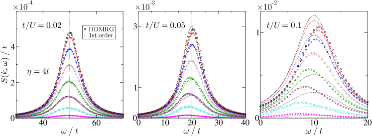
Figure 1: Frequency dependence of the dynamical charge structure factor $S(k,\omega)$ at various momenta $k=2\pi j/L$ (for $j=1,2,\ldots,L/2$ from bottom to top). DDMRG data (symbols) were obtained for $L=16$; $S^{(1)}_{\eta}(k,\omega)$ (lines) give the corresponding first-order strong-coupling expansion results (for the same value of $\eta=4t$). The dashed line indicates the point $\omega=U$.

From lowest-order strong-coupling perturbation theory we find for $\rho=N/L=1$ ($N,L\to\infty$)

$$S^{(1)}(k,\omega>0)=\left(\frac{4t\sin(k/2)}{U}\right)^{2}\int_{-\pi}^{\pi}\frac{{\rm d}k}{\pi}\sin^{2}k\,\delta(\omega-U+2t\cos k\sqrt{5+4\cos k})\,.$$ (3)

Then, for $U-2\sqrt{5+4\cos k}\leq\omega\leq U+2\sqrt{5+4\cos k}$, we have in units of $t$

$$S^{(1)}(k,\omega>0)=\left[\frac{4\sin(k/2)}{U}\right]^{2}\frac{\sqrt{20+16\cos k-(\omega-U)^{2}}}{2\pi(5+4\cos k)}\,,$$ (4)

where $0\leq k<2\pi$. Since DDMRG provides $S(k,\omega)$ with a finite broadening $\eta$, it is useful to convolve the strong-coupling result $S^{(1)}(k,\omega)$ with the Lorentz distribution [10]: $S_{\eta}(k,\omega)=\int_{-\infty}^{\infty}{\rm d}\omega^{\prime}S(k,\omega^{\prime})\eta/\left[\pi\left[(\omega-\omega^{\prime})^{2}+\eta^{2}\right]\right]$. For the 1D BHM, from Eq. (4), we thus get

$$S_{\eta}^{(1)}(k,\omega>0)=\left(\frac{4\sin(k/2)}{U}\right)^{2}\frac{2}{\pi^{2}}\int_{-1}^{1}{\rm d}\lambda\frac{\eta\sqrt{1-\lambda^{2}}}{(\omega-U+2\lambda\sqrt{5+4\cos k})^{2}+\eta^{2}}\,.$$ (5)

Figure 1 illustrates the frequency and momentum dependencies of $S(k,\omega)$. Peaks in $S(k,\omega)$ assign charge excitations. For $k\simeq 0$, $S(k,\omega)$ exhibits a maximum around $\omega\approx U$ that can be attributed to excitations across the Mott gap. Within strong-coupling theory (4) this signature stays at $\omega\approx U$ for all $k$ but becomes more pronounced as $k$ reaches the Brillouin zone boundary. Our DDMRG data corroborate this prediction (cf. the left panel of Fig. 1 depicting the results for $t/U=0.02$). Naturally, as $U$ gets smaller, differences between the numerical DDMRG and the analytical strong-coupling results emerge. Most importantly, the position of the maximum in $S(k,\omega)$ varies with $k$: it is shifted to smaller (larger) frequencies for $k$ values near the band centre (Brillouin zone boundary); see middle and right-hand panels of Fig. 1. We have to include higher-order $t/U$–corrections to reproduce this feature analytically. Note that the maximum in $S(k,\omega)$ amplifies as $k\to\pi$.

Next, we investigate the dependences of $S(k,\omega)$ on the broadening $\eta$ and the system size $L$ to scrutinise whether the DDMRG data “converge” to the unconvolved strong-coupling result (4) as $\eta\to 0$ and $L\to\infty$. Figure 2—showing $S(k,\omega)$ in the MI phase at $k=\pi/8$ (left), $\pi/2$ (middle) and $\pi$ (right panel) for $L=16$, 32, 64 $\eta=4t$, $2t$, $t$, respectively—demonstrates that this is indeed the case. Firstly, for $t/U=0.02$, we see that the DDMRG results are in a satisfactory accord with $S_{\eta}^{(1)}(k,\omega)$, where as a matter of course for smaller system sizes a larger value of $\eta$ has to be used to achieve good agreement. Secondly, $S(k,\omega)$ calculated by DDMRG approaches the curve given by (4) for increasing system size $L$ and decreasing broadening $\eta$.

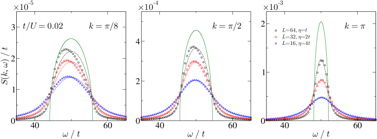
Figure 2: $\eta$-dependence of the dynamical structure factor $S(k,\omega)$. DDMRG data (symbols) are compared with the corresponding strong-coupling results (dashed lines) at various momenta $k$. The solid green line shows the unconvolved result of the strong-coupling expansion.

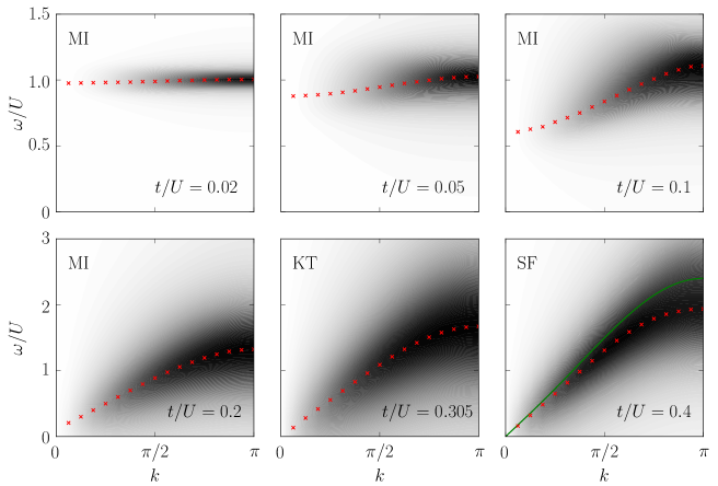
Figure 3: Intensity of the dynamical structure factor $S(k,\omega)$ in the $k$–$\omega$ plane for different $t/U$. DDMRG data were obtained for $L=32$ system, using $\eta=2t$ ($\eta=t$) in the MI phase and at the KT transition point (in the SF phase). The red crosses mark the positions of the maximum in each $k=2\pi j/L$–sector. The green line for $t/U=0.4$ marks the field-theory/Bogoliubov result $\omega(k)=\sqrt{\epsilon_{0}(k)[\epsilon_{0}(k)+2U]}$ with $\epsilon_{0}(k)=-2t(\cos k-1)$.

Finally, we look at the changes in the dynamical density-density response as the system crosses the MI-SF quantum phase transition with decreasing Coulomb interaction strength. Figure 3 shows the intensity distribution of $S(k,\omega)$ in the MI and SF phases as well as in the vicinity of the Kosterlitz–Thouless (KT) transition point, where the charge excitation gap closes. For large $U$, the spectral weight is mainly concentrated around $\omega=U$ in the region $\pi/2\leq k\leq\pi$, in agreement with the strong-coupling prediction. As $U$ weakens in the MI phase, the distribution of the spectral weight broadens. At the same time, the maximum value of $S(k,\omega)$ acquires a sizable dispersion (see upper-row panels). As the system reaches the MI-SF transition point we observe a significant redistribution of spectral weight to lower $k$ values and, most notably, the excitation gap closes (see lower panels). In our previous work, we evaluated the scaling of the Tomonaga–Luttinger liquid parameter and determined the KT transition point to be located at $t/U=0.305(1)$ [3]. In the SF phase spectra for $k\gtrsim 0$ (cf. the panel for $t/U=0.4$), we observe an almost linear dispersion of the $S(k,\omega)$, which—in accordance with bosonization [11] and with Bogoliubov theory [12] —can be taken as a signature of the Bose condensation process. Our 1D DDMRG BHM data are unsuggestive of two distinct (gapless sound and massive) modes in the SF phase. These two phases are found in mean-field theory and may appear for dimensions $d\geq 2$ where a true condensate exists in the SF ground state.

To summarise, we have determined the dynamical structure factor $S(k,\omega)$ for the 1D BHM with particle density $\rho=N/L=1$ by means of unbiased numerical DDMRG calculations. As discussed for photoemission spectra previously [3], $S(k,\omega)$ agrees with the first-order perturbation theory result in the Mott insulator phase for $U\gg t$. Naturally, as the Coulomb interaction is lowered, noticeable deviations appear between both approaches, in particular the DDMRG $S(k,\omega)$ becomes dispersive and we find a substantial redistribution of spectral weight into the small $k$-sector. In this regime, higher-order corrections have to be taken into account in our analytical treatment of the BHM. Approaching the SF state, the charge excitations gap closes and the maximum in $S(k,\omega)$ exhibits a linear dispersion. The quantum phase transition between MI and SF phases is located at about $t/U\simeq 0.3$ and found to be of KT type.

Acknowledgements. SE and HF acknowledge funding by DFG through SFB 652.

References

References

- [1] Greiner M, Mandel O, Esslinger T, Hänsch T W and Bloch I 2002 Nature 415 39
- [2] Bloch I, Dalibard J and Zwerger W 2008 Rev. Mod. Phys. 80 885
- [3] Ejima S, Fehske H and Gebhard F 2011 Europhysics Letters 93 3002
- [4] Oosten D van et al. 2005 Phys. Rev. A 71 021601(R)
- [5] Huber S D, Altman E, Büchler H P and Blatter G 2007 Phys. Rev. B 75 085106
- [6] Roth R and Burnett K 2004 J. Phys. B 37 3893
- [7] Pippan P, Evertz H G and Hohenadler M 2009 Phys. Rev. A 80 033612
- [8] White S R 1992 Phys. Rev. Lett. 69 2863; Jeckelmann E 2002 Phys. Rev. B 66 045114
- [9] Stenger J et al. 1999 Phys. Rev. Lett. 82 4569
- [10] Nishimoto S and Jeckelmann E 2004 J. Phys.:Condens. Matter 16 613
- [11] Cazalilla M A, Citro R, Giamarchi T, Orignac E and Rigol M, 2011 Rev. Mod. Phys. 83 1405
- [12] Bogoliubov N N 1947 J. Phys. (USSR) 11 23