Modelling Herschel observations of hot molecular gas emission from embedded low-mass protostars

Abstract

Aims. Young stars interact vigorously with their surroundings, as evident from the highly rotationally excited CO (up to $E_{\rm u}/k=4000$ K) and H₂O emission (up to 600 K) detected by the Herschel Space Observatory in embedded low-mass protostars. Our aim is to construct a model that reproduces the observations quantitatively, to investigate the origin of the emission, and to use the lines as probes of the various heating mechanisms.

Methods. The model consists of a spherical envelope with a power-law density structure and a bipolar outflow cavity. Three heating mechanisms are considered: passive heating by the protostellar luminosity, ultraviolet irradiation of the outflow cavity walls, and small-scale C-type shocks along the cavity walls. Most of the model parameters are constrained from independent observations; the two remaining free parameters considered here are the protostellar UV luminosity and the shock velocity. Line fluxes are calculated for CO and H₂O and compared to Herschel data and complementary ground-based data for the protostars NGC1333 IRAS2A, HH 46 and DK Cha. The three sources are selected to span a range of evolutionary phases (early Stage 0 to late Stage I) and physical characteristics such as luminosity and envelope mass.

Results. The bulk of the gas in the envelope, heated by the protostellar luminosity, accounts for 3–10% of the CO luminosity summed over all rotational lines up to $J=40$–39; it is best probed by low-$J$ CO isotopologue lines such as C¹⁸O 2–1 and 3–2. The UV-heated gas and the C-type shocks, probed by ¹²CO 10–9 and higher-$J$ lines, contribute 20–80% each. The model fits show a tentative evolutionary trend: the CO emission is dominated by shocks in the youngest source and by UV-heated gas in the oldest one. This trend is mainly driven by the lower envelope density in more evolved sources. The total H₂O line luminosity in all cases is dominated by shocks ($>99\%$). The exact percentages for both species are uncertain by at least a factor of 2 due to uncertainties in the gas temperature as function of the incident UV flux. However, on a qualitative level and within the context of our model, both UV-heated gas and C-type shocks are needed to reproduce the emission in far-infrared rotational lines of CO and H₂O.

1 Introduction

In the embedded phases of low-mass star formation (Stages 0 and I; Whitney et al., 2003; Robitaille et al., 2006), the material surrounding the protostar is exposed to energetic phenomena such as shocks and ultraviolet radiation (Shu et al., 1987; Spaans et al., 1995; Bachiller & Tafalla, 1999; Arce et al., 2007). Observationally, this leads to much higher intensities in lines of rotationally excited carbon monoxide, water and other species than would be possible from gas that is only heated through collisions with warm dust in the bulk of the envelope. The ubiquity of surplus rotationally excited emission was first established through ground-based observations of the CO $J=6$–5 transition (upper-level energy $E_{\rm u}/k=120$ K; Schuster et al., 1993; Hogerheijde et al., 1998). The Infrared Space Observatory (ISO) subsequently detected CO up to the 21–20 line ($E_{\rm u}/k=1300$ K), along with rotationally excited H₂O (up to 470 K) and OH (up to 620 K; Ceccarelli et al., 1999; Giannini et al., 1999, 2001; Nisini et al., 2002). The origin of this hot gas has been debated ever since. The shape of the CO 6–5 spectra – a narrow emission feature on top of a broader one – and the presence of a strong, narrow ¹³CO 6–5 emission feature point at a mixture of quiescent and shocked gas, with the quiescent gas likely heated by the protostellar UV field along the cavity walls (Spaans et al., 1995). Spatially resolved CO 6–5 maps, showing extended narrow emission, provide additional support for this scenario (van Kempen et al., 2009). However, it remains unclear at a quantitative level to what extent UV radiation and shocks each contribute to heating up the gas and powering the emission.

The Herschel Space Observatory (Pilbratt et al., 2010) offers a new set of tools to tackle this question. Amongst its first results are detections of highly rotationally excited CO (up to $J=38$–37, $E_{\rm u}/k=4100$ K) and H₂O (up to 640 K) in the embedded low-mass protostars HH~46 and DK~Cha (van Kempen et al., 2010a, b). A quantitative radiative transfer model of HH 46 was successful at explaining the CO line fluxes with a combination of UV-heated gas in the outflow cavity walls and small-scale C-type shocks along the walls (van Kempen et al., 2010b). However, the model was unable to disentangle the origin of the observed H₂O lines in a similar fashion. The goals of the current paper are (1) to present our model from van Kempen et al. in more detail; (2) to check how robust the model fit is for CO; (3) to derive a quantitative fit for H₂O; and (4) to extend the analysis to DK Cha and a third source (NGC1333 IRAS2A) for which CO and H₂O data have since become available (Kristensen et al., 2010; Yıldız et al., 2010). The three test cases are all nearby protostars ($d=180$–450 pc) and cover the evolutionary range from deeply embedded Stage 0 to late Stage I.

The question of the origin of the hot gas observed with Herschel is not limited to embedded low-mass young stellar objects (YSOs). Herschel observations of rotationally excited CO and/or H₂O include intermediate-mass YSOs (Fich et al., 2010; Johnstone et al., 2010), high-mass YSOs (Chavarría et al., 2010), circumstellar disks (Meeus et al., 2010; Sturm et al., 2010), the Orion Bar photon-dominated region (Habart et al., 2010), and even extragalactic sources like the ultraluminous infrared galaxy Mrk~231 (van der Werf et al., 2010). A quantitative explanation of the origin of the observed emission is still missing in most of these cases. Our model may help in constraining possible excitation mechanisms in environments other than low-mass YSOs. In particular, the treatment of how the gas is excited by UV fields and shocks can be adapted for different types of sources.

This work is part of the two complementary Herschel Key Programmes WISH and DIGIT. The primary goal of WISH, or “Water in star-forming regions with Herschel” (van Dishoeck et al., 2011), is to use H₂O as a probe of the physical and chemical conditions during star formation and to follow its abundance as a function of evolutionary phase. DIGIT, or “Dust, ice, and gas in time” (PI: N. Evans), aims to study the evolution of the gas during different stages of star formation, as well as that of the dust grains and their icy mantles. Observations of CO are an integral part of both programmes, because its simple chemistry and easy use in radiative transfer codes make CO an excellent tool to constrain physical conditions and processes. Indeed, the approach in the current paper is to fit the free parameters in the model to the CO data and then to assess how well the model reproduces the H₂O data. More generally, the model is ultimately intended as a tool in using the Herschel data as a probe of the energetics and dynamics of star formation, in particular how and where the young star deposits energy back into the parent molecular cloud. Future work in WISH and DIGIT will explore these questions in more detail.

A detailed description of the model appears in Sect. 2. The Herschel data and complementary ground-based data are summarised in Sect. 3. The model results for CO and H₂O are presented in Sect. 4 and discussed in Sect. 5. Conclusions are drawn in Sect. 6.

2 Model description

The far-infrared (far-IR) and sub-millimetre (sub-mm) molecular line emission from embedded low-mass protostars has traditionally been interpreted with purely spherical envelope models, but such models cannot reproduce the observed intensities of rotationally excited lines like CO 6–5 and higher (e.g., van Kempen et al., 2009). Our model goes a step further by introducing a bipolar outflow cavity with two additional heating mechanisms: UV irradiation of the gas in the cavity walls and small-scale C-type shocks along the walls (Fig. 1). Rotationally excited emission may also arise from the bipolar jet and the associated internal J-type shocks, from gas heated by X-rays, or from a circumstellar disk embedded within the envelope. However, our goal is not to create a single all-inclusive model of an embedded protostar. Rather, the main question in this work is what the Herschel observations can teach us about the passively heated envelope, the UV-heated cavity walls and the small-scale shocks. Investigating the quantitative contributions from other components will be left for future studies. Furthermore, the current focus is on the integrated line intensities only. With regards to the Herschel-PACS data, we are only interested in the emission from the central spaxel of the full $5\times 5$ spaxel array. Future updates of the model will explore the spatial extent of the emission and could add dynamical processes to allow for the computation of line profiles.

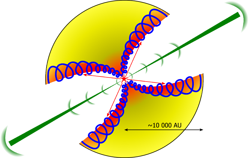
Figure 1: Schematic view of the physical components in an embedded Stage 0 or I young stellar object: a passively heated envelope (yellow, with a hot core shaded red), a bipolar jet (green, with bow shocks and internal working surfaces), UV-heated outflow cavity walls (red), and small-scale shocks along the cavity walls (blue). Not visible on this scale is an embedded circumstellar disk with a radius of $\sim$100 AU.

2.1 Passively heated envelope

Low-$J$ lines from CO and its isotopologues and similar low-excitation lines from other species are commonly modelled with a spherical envelope (e.g., Jørgensen et al., 2002; Schöier et al., 2002). A spherical envelope is also the starting point of our model, since the warm inner region can contribute to emission in the higher-$J$ lines. The gas in the envelope is well coupled to the dust and is only heated passively or indirectly, i.e., the dust is heated by the protostellar luminosity and the gas attains the same temperature through collisions with the dust.

The density and temperature profiles of each source are constrained from continuum observations. Following the method of Jørgensen et al. (2002) and Schöier et al. (2002), the continuum emission for a grid of envelope models is calculated with the 1D continuum radiative transfer program DUSTY (Ivezić et al., 1999). The best-fit model is determined by comparing the emission to spectral energy distributions (SEDs) and sub-mm brightness profiles compiled by Froebrich (2005) and Di Francesco et al. (2008). The inner radius of the envelope is set at a dust temperature of 250 K (about 30 AU or $0.15^{\prime\prime}$ at 200 pc; Table 2). If any material is present on smaller scales, its contribution to the overall line emission would be too diluted in the $\sim$$10^{\prime\prime}$ Herschel beam to have a significant impact on the model results. The envelopes are optically thick at UV and visible wavelengths, so most of the stellar radiation is reprocessed by the dust. For a constant stellar luminosity, the assumed stellar temperature therefore does not have a significant effect on the resulting dust temperatures or the molecular line emission (Jørgensen et al., 2002). This was verified by running part of the DUSTY grid for stellar temperatures of both 5 000 and 10 000 K.

The remaining three free parameters are fitted in a $\chi^{2}$ procedure: the power-law index for the density profile ($n\propto r^{-p}$), the optical depth at 100 $\mu$m ($\tau_{100}$), and the size of the envelope ($Y\equiv r_{\rm out}/r_{\rm in}$). For our line radiative transfer models, the envelopes are terminated at the point where the density reaches $10^{3}$ cm^-3 or the temperature reaches 10 K (Jørgensen et al., 2002). This point is denoted $r_{\rm env}$. The best-fit values for the three test cases are listed in Table 2 in Sect. 3, and the associated density and temperature profiles are plotted in Fig. 5.

The Doppler broadening parameter $b$ for the passive envelope models is fixed at 0.8 km s^-1, a typical value for the quiescent gas in low-mass YSOs as determined from optically thin C¹⁸O observations (Jørgensen et al., 2002). The ongoing collapse of the envelope onto the star and disk is simulated with a power-law infall velocity profile $\varv\propto r^{-1/2}$ (Shu, 1977), scaled to 2.0 km s^-1 at the inner edge of the envelope. Details on how the abundances are obtained and how the molecular line intensities are calculated are provided in Sects. 2.2.2 and 2.2.3.

2.2 Photon-heated cavity walls

2.2.1 Density and temperature

The second model component is the UV-heated gas in the walls of the outflow cavities (red in Fig. 1; Spaans et al., 1995; van Kempen et al., 2009). For an ambient cavity density of a few $10^{3}$ cm^-3 (Neufeld et al., 2009), the total gas column from the central source to the point where the cavity intersects the outer edge of the envelope (a distance of $\sim$$10^{17}$ cm) is a few $10^{20}$ cm^-2. This corresponds to a UV optical depth of a few tenths, so UV photons produced near the protostar can freely reach the cavity walls. When they do, they produce a photon-dominated zone where the gas is heated to temperatures of a few hundred K.

The first step in modelling the emission from the UV-heated gas is to carve out a bipolar cavity from the spherical envelope, similar to the procedure followed by Bruderer et al. (2010). Mid-infrared Spitzer Space Telescope images of HH 46 and similar YSOs like L~1527 show ellipsoidal cavities, with a ratio between the semimajor and semiminor axes ($a_{\rm cav}$ and $b_{\rm cav}$) of about 4 (Velusamy et al., 2007; Tobin et al., 2008). Large-scale CO 3–2 maps of NGC1333 IRAS2A, tracing the swept-up outflow gas, show roughly the same shape (Sandell et al., 1994). DK Cha is oriented close to pole-on (Knee, 1992), so the shape and size of its outflow are unknown.

Tests of our model show that the variation in the computed CO and H₂O line fluxes resulting from changes in the shape and size of the cavities is within the overall model uncertainties, consistent with the more detailed tests of Bruderer et al. (2010). Our approach is therefore to fix the ratio between the outflow axes ($a_{\rm cav}/b_{\rm cav}$) of all three sources to the value of 4.3 measured for HH 46 (Velusamy et al., 2007), and to scale the absolute length of the axes with the envelope radius. In other words, the ratios $a_{\rm cav}/r_{\rm env}$ and $b_{\rm cav}/r_{\rm env}$ of all three sources are fixed to the values of 2.1 and 0.50 derived for HH 46. The envelope radii and outflow axis lengths are summarised in Table 2.

The two cavities for each source are aligned along the $z$ axis, with the ends meeting at $z=0$ (Fig. 2). The ellipsoidal cavity wall in the upper right quadrant of a cylindrical coordinate system is defined as

$$R_{\rm cav}=b_{\rm cav}\sqrt{1-\left(\frac{z_{\rm cav}}{a_{\rm cav}}-1\right)^{2}}\,.$$ (1)

The points along the wall can also be characterised by their distance $r_{\rm cav}$ to the protostar,

$$r_{\rm cav}=\sqrt{R^{2}_{\rm cav}+z^{2}_{\rm cav}}\,,$$ (2)

which is used for some figures in Sect. 4.

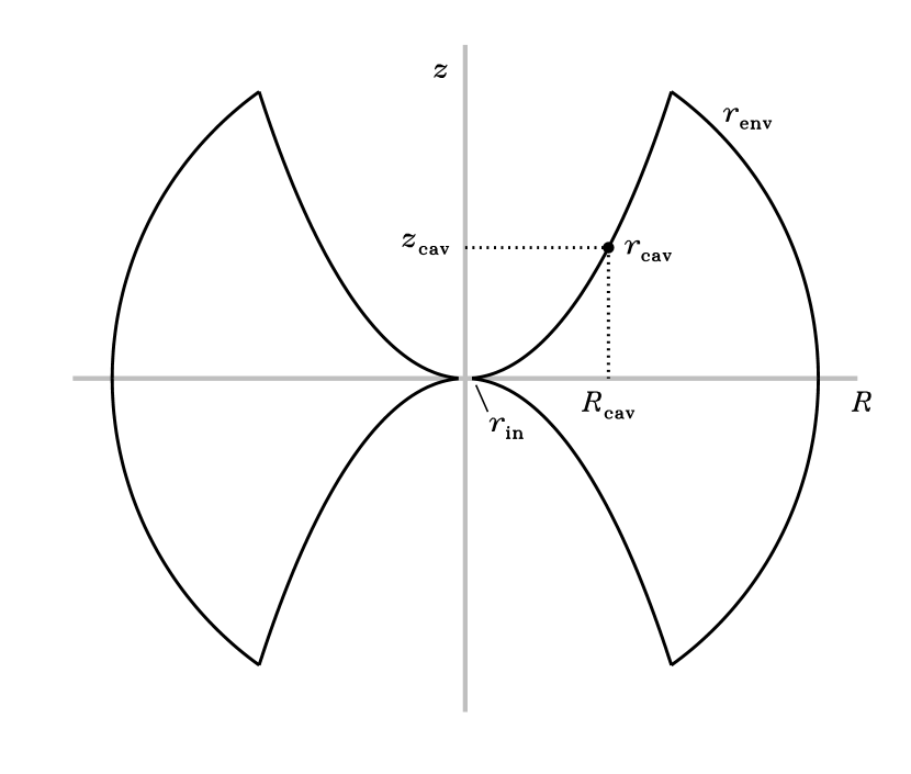
Figure 2: Schematic view of the envelope and the bipolar outflow cavity. In each quadrant, a point on the cavity wall is uniquely identified by its distance $r_{\rm cav}$ to the central star at the origin (Eq. (2)).

The only UV source included in our model is the protostar. UV photons can also be produced at the bow shock (Böhm et al., 1993; Raymond et al., 1997) or by small-scale shocks within the cavity or along the walls (Curiel et al., 1995; Saucedo et al., 2003; Walter et al., 2003), but these contributions are highly uncertain. The protostellar UV luminosity itself is also highly uncertain, and is therefore treated as a free parameter. Classical T Tauri stars have typical $L_{\rm UV}$ of $10^{-3.5}$–$10^{-1.5}$ times the total stellar luminosity (Ingleby et al., 2011). Scaling up to the higher accretion rates found in embedded YSOs, anything from 0.01 to 1 $L_{\odot}$ would be a reasonable value for our model. The best-fit UV luminosities derived in Sect. 4.2 range from $<$0.03 to 0.08 $L_{\odot}$. An $L_{\rm UV}$ of 0.1 $L_{\odot}$ would give an unattenuated UV flux at 100 AU of $G_{0}\approx 10^{4}$ relative to the mean interstellar radiation field of Habing (1968).

Due to the UV field impinging on the cavity walls, the gas is heated to higher temperatures than it attains in the passively heated, purely spherical envelope. The temperature can be calculated by solving the heating and cooling balance as function of the physical conditions. Many such models are available in the literature, but they show substantially different results, sometimes even at the qualitative level (Röllig et al., 2007). The consequences of these uncertainties for our model results are discussed extensively in Sect. 5.1. For the initial results in Sect. 4, the PDR surface temperature grid of Kaufman et al. (1999) is adopted as our standard prescription. This grid was calculated for densities up to $10^{7}$ cm^-3; for higher densities, it is extrapolated as $1/n({\rm H}_{2})$ based on the expected dominant heating and cooling mechanisms (Sect. 5.1).

The Kaufman et al. (1999) grid as such can only be used at the cavity wall. At any depth into the envelope, the temperature needs to be corrected for attenuation of the UV field by dust. Röllig et al. (2007) plotted the temperature as function of the visual extinction, $A_{\rm V}$, for several densities and unattenuated UV fluxes. In each case, the temperature decreases roughly as $\exp(-0.6A_{\rm V})$. In order to use this depth dependence in our model, the amount of extinction towards any point ($R,z$) is calculated with the continuum radiative transfer code RADMC (Dullemond & Dominik, 2004). The input stellar spectrum is a 10 000 K blackbody scaled to a given UV luminosity between 6 and 13.6 eV. This input spectrum is a reasonable approximation of the real spectrum emitted by a low-mass protostar with a UV excess due to accretion (e.g., van Zadelhoff et al., 2003). The local UV flux from RADMC, $F_{\rm RADMC}$ (also integrated from 6 to 13.6 eV), can be considered the product of the unattenuated flux and an extinction term,

$$F_{\rm RADMC}(R,z)=F_{\rm unatt}\exp(-\tau_{\rm UV})\,,$$ (3)

where $F_{\rm unatt}$ is the UV flux through a unit surface arising from a source at a distance $\sqrt{R^{2}+z^{2}}$. The UV optical depth, $\tau_{\rm UV}$, is effectively an average over the many possible paths a photon can follow from the source to the point ($R,z$). It is converted into a visual extinction via $A_{\rm V}=\tau_{\rm UV}/3.02$ (Bohlin et al., 1978). Along with the UV field, RADMC also calculates the dust temperature along the cavity wall and throughout the envelope. This is used instead of the dust temperature from the 1D DUSTY models.

One caveat with RADMC is that it treats scattering of the radiation by dust as an isotropic process, while in reality grains are partially forward scattering (Li & Draine, 2001). Tests with the radiative transfer code of van Zadelhoff et al. (2003), which does allow for anisotropic scattering, show flux differences of at most 20% between an isotropic scattering function and the scattering function of Li & Draine. This is within our overall model uncertainty.

The present goal is to reproduce the observed integrated line fluxes, not the detailed line profiles. Hence, the Doppler broadening and infall velocities for the UV-heated component are kept the same as in the passively heated component.

2.2.2 Abundances

Several thousand grid points are required to properly sample the envelope and the cavity walls in the 3D radiative transfer calculations (Sect. 2.2.3). It would be too time consuming to calculate the abundances of CO and H₂O for each individual point with a traditional chemical code. Instead, the abundances are obtained according to the method of Bruderer et al. (2009). A grid of chemical models is pre-computed for the appropriate range of densities, temperatures, unattenuated UV fluxes and extinctions. Abundances for each individual point in the envelope or the cavity wall are interpolated from this grid when constructing the source models for the radiative transfer code.

The basis of our chemical reaction network is the UMIST06 database (Woodall et al., 2007) as modified by Bruderer et al. (2009), except that X-ray chemistry is not included. The network allows all neutrals to freeze out onto the dust to account for the depletion of many gas-phase species in the colder parts of the envelope. Molecules can return to the gas phase through thermal desorption and photodesorption. Binding energies and photodesorption yields for CO and H₂O are taken from Fraser et al. (2001), Bisschop et al. (2006) and Öberg et al. (2007, 2009). Photodesorption occurs even in regions of high extinction because of a cosmic-ray–induced UV flux of about $10^{4}$ photons cm^-2 s^-1, equivalent to $10^{-4}$ times the mean interstellar flux (Shen et al., 2004). In the gas phase, UV photons can dissociate or ionise many species; the relevant rates are calculated according to van Dishoeck et al. (2006) for a 10 000 K blackbody stellar spectrum, appropriate for a low-mass protostar with a UV excess. Self-shielding of H₂ and CO, which causes their dissociation rates to decrease more rapidly than those of other species, is included according to Draine & Bertoldi (1996) and Visser et al. (2009). The cosmic-ray ionisation rate of H₂ is set to $5\times 10^{-17}$ s^-1 (Dalgarno, 2006).

The grid of pre-computed abundances, from which abundances for the three sources are interpolated, is obtained by advancing the chemical reactions for a period of $10^{5}$ yr. As starting conditions, all carbon is locked up in CO, the remaining oxygen in H₂O, all nitrogen in N₂, and all remaining hydrogen in H₂. Reflecting the most likely formation pathways, CO and N₂ start in the gas phase, while H₂O starts frozen out on the dust. H₂ is predominantly formed on the grains, but because it rapidly evaporates even at 10 K, it starts in the gas phase. Elemental abundances are adopted from Aikawa et al. (2008) and Bruderer et al. (2009); the initial composition is summarised in Table 1.

Table 1: Initial abundances of molecules in our chemical grid.

Species	Abundance
H2	1.00(0)$-$
CO	1.57($-$4)
H2Oice	2.03($-$4)
N2	4.94($-$5)

2.2.3 Radiative transfer

Level populations and line intensities for the passively heated envelope and the UV-heated outflow cavity walls are calculated with the new full-3D radiative transfer code LIME (Brinch & Hogerheijde, 2010). LIME uses an irregular grid with points sampled randomly but weighted according to a user-defined criterion such as density or temperature. This naturally results in a finely spaced grid in the regions most important for the astrophysical problem at hand.

The source geometry of our models introduces a substantial difficulty: the high-excitation CO and H₂O lines originate in a thin layer of hot gas along the cavity wall, so an accurate flux calculation requires a high grid point density inside and immediately outside this small region. Furthermore, the grid has to be able to resolve emission on scales ranging from $\sim$10 to $\sim$$10^{4}$ AU. This cannot be accomplished with the default density or temperature weighting functions. Extensive convergence tests were carried out to find an alternative grid sampling scheme. The optimised grid consists of 30 000 points, picked randomly in $\log{r}$ between $r_{\rm in}$ and $r_{\rm env}$. For every point with radial coordinate $r$, a point ($R_{\rm cav},z_{\rm cav}$) is located on the cavity wall such that $\sqrt{R_{\rm cav}^{2}+z_{\rm cav}^{2}}=r$. Let $\gamma_{\rm cav}$ be the angle between the point ($R_{\rm cav},z_{\rm cav}$) and the midplane, i.e., $\tan{\gamma_{\rm cav}}=z_{\rm cav}/R_{\rm cav}$. The angular coordinate $\gamma$ of each point is then determined as follows:

1. one third of the points are placed exactly at the cavity wall ($\gamma=\gamma_{\rm cav}$);

2. one third of the points are picked with a random angle $\gamma$ such that $0.9<\gamma/\gamma_{\rm cav}\leq 1$;

3. one third of the points are picked with a random angle $\gamma$ such that $0<\gamma/\gamma_{\rm cav}\leq 1$ and then weighted by $\sqrt{\gamma/\gamma_{\rm cav}}$, which favors points near the midplane over points near the cavity wall.

The grid thus constructed is smoothed by five iterations of Lloyd’s algorithm (Lloyd, 1982), which moves each point somewhat towards the centre of mass of its Voronoi cell. The purpose of this smoothing step is two-fold: (1) to turn some “needle-shaped” cells created by the random setup into more regular shapes (Brinch & Hogerheijde, 2010); and (2) to push some grid points from the first sampling group into the cavity wall, so that the edge between the envelope and the cavity is well sampled on either side. The first two groups of points together cover the region of hot gas responsible for the more excited lines. The third group of points covers the bulk of the envelope, where the low-$J$ emission originates.

With the grid established, LIME employs the standard two-step method for problems where local thermodynamic equilibrium (LTE) does not apply. The first step is an iterative procedure to calculate the rotational level populations based on the balance between radiative excitation, collisional excitation and collisional de-excitation. The second step is the ray tracing, i.e., calculating the emergent spectrum at a given distance and inclination. The collisional rate coefficients required for the first step are collected from the Leiden Atomic and Molecular Database (LAMDA; Schöier et al., 2005), where the most recent data files for CO and H₂O are from Yang et al. (2010) and Faure et al. (2007), respectively. The ortho-to-para ratio for H₂ is taken to be thermalised, with a maximum value of 3. The ortho-to-para ratio of H₂O is fixed at 3. Dust is included in the model with a standard gas-to-dust ratio of 100 and the OH5 opacities from Ossenkopf & Henning (1994), appropriate for dust grains with a thin ice mantle.

Images are created at 0$\aas@@fstack{\prime\prime}$1 resolution (18–45 AU at the distances of the three sources; Table 2) to get a sufficiently fine sampling of the hot inner regions. In order to compare the model results to the observations, each image is convolved with a Gaussian beam profile. Beam sizes are calculated as the diffraction-limited beam for the wavelength and the telescope (Herschel, APEX or JCMT) at which the simulated line was observed. In the case of lines observed with Herschel-PACS, fluxes are extracted from the central $9\aas@@fstack{\prime\prime}4\times 9\aas@@fstack{\prime\prime}4$ to mimic the instrument’s central spaxel. For a given density, temperature and abundance structure, the estimated uncertainty on the CO line fluxes ranges from 30% for the 2–1 line to a factor of 2 for the high-$J$ end of the ladder. For H₂O, it is a factor of 2 for all lines. The uncertainty is mainly due to the complex geometry and the small size of the emitting region for the high-$J$ lines. The source models themselves lead to uncertainties of similar magnitude in the line fluxes, mostly because of the problems with the gas temperature discussed in Sect. 5.1.

Integrated intensities from APEX, the JCMT and Herschel-HIFI ($\int T_{\rm mb}{\rm d}\varv$ in K km s^-1) and integrated fluxes from Herschel-PACS ($\int F_{\nu}{\rm d}\nu$ in W m^-2) can be mutually converted through

$$\int F_{\nu}{\rm d}\nu=\frac{2k\Omega}{\lambda^{3}}\int T_{\rm mb}{\rm d}\varv\,,$$ (4)

with $\Omega(\lambda)$ the solid angle subtended by the beam at the given wavelength. Denoting the full width at half maximum (FWHM) of the beam as $\Theta(\lambda)$, the solid angle for APEX, the JCMT and HIFI is $(\pi/4\ln 2)\Theta^{2}$. The formula is more complicated for PACS, because the size of the spaxels has to be taken into account. For just the central spaxel, the solid angle is

$$\Omega_{\rm PACS}(\lambda)=\left[\frac{9\aas@@fstack{\prime\prime}4}{{\rm erf}\left(9\aas@@fstack{\prime\prime}4\sqrt{\ln{2}}/\Theta\right)}\right]^{2}\,,$$ (5)

with erf the error function and $\Theta(\lambda)$ the FWHM of the diffraction-limited Herschel beam.

2.3 Small-scale shocks

The third model component is a series of C-type shocks moving along the cavity walls. These shocks may be powered by the wind launched from close to the protostar or the surface of the inner disk, or by the expansion of the jet (e.g., Lada, 1985; Shang et al., 2006; Arce & Sargent, 2006; Santiago-García et al., 2009). Shocks are created when the wind hits the outflow cavity walls, heating the gas to temperatures of more than 1000 K.

The model procedure is the same as that of Kristensen et al. (2008), except for a change in the geometry. In the original procedure, 1D shock model results were pasted along a parabola to simulate emission from a bow shock observed in H₂ in the Orion Molecular Cloud. Here, in order to simulate C-type shocks along the cavity walls, the 1D shocks are pasted along the ellipsoids from Sect. 2.2.1. The shock velocity is assumed to be constant along the entire length of the wall and the pre-shock density is that of the envelope at the given distance from the protostar. The magnetic field is set to $\beta[2n({\rm H}_{2})/{\rm cm}^{-3}]^{1/2}$, with $\beta$ fixed at 1 $\mu$Gauss. Abundances as function of depth into the shock are calculated from a limited chemical network centred on H₂O (Wagner & Graff, 1987), which does not include photodissociation or other UV-driven reactions.

The shock model results of Kaufman & Neufeld (1996) are used in combination with the model results of Flower & Pineau des Forêts (2003) and Kristensen et al. (in prep.) to compute the emergent line intensities. The first step is to estimate the extent of the line-emitting region by measuring the FWHM of the cooling-rate profile of the relevant molecule through the shock. The bottom panel of Fig. 3 shows the cooling profiles from Flower & Pineau des Forêts for CO and H₂O, for a shock velocity of 20 km s^-1 and pre-shock densities of $10^{4}$ and $10^{6.5}$ cm^-3. The corresponding temperature and abundance profiles are plotted in the top panel. CO and H₂O cool the same part of the shock and their cooling lengths are nearly the same. Furthermore, the cooling lengths are nearly inversely proportional to the pre-shock density, i.e., the solid and dotted profiles look similar but are shifted on the logarithmic scale. The cooling lengths provide an estimate of the extent over which the shock is emitting, and as such are an effective measure of the beam-filling factor.

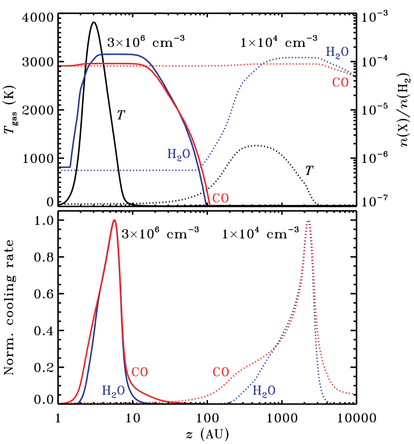
Figure 3: Top: Temperature of the neutral gas (black) and abundances of CO (red) and H₂O (blue) as function of depth into a shock for a shock velocity of 20 km s^-1 and pre-shock densities of $3\times 10^{6}$ (solid) and $1\times 10^{4}$ cm^-3 (dotted). Bottom: Normalised cooling rates of CO and H₂O for the same two sets of conditions. All data are taken from the models of Flower & Pineau des Forêts (2003).

The second step is to divide the cavity wall into discrete segments according to the envelope density. The upper limit of the Kaufman & Neufeld (1996) grid is $10^{6.5}$ cm^-3; the pre-shock density for the denser parts of the envelope is set to that value. Figure 4 shows the adopted segmentation for HH 46; the width of the coloured area is a rough representation of the size of the emitting region. The CO and H₂O line intensities are estimated from the results tabulated by Kaufman & Neufeld. The emission is assumed to fill each of the segments, thus creating an emission map for each line. Just like the raw images produced by LIME (Sect. 2.2.3), the maps are convolved with a Gaussian beam profile of the appropriate diameter. For lines observed with Herschel-PACS, the flux is extracted from the central $9\aas@@fstack{\prime\prime}4\times 9\aas@@fstack{\prime\prime}4$. The fluxes are not corrected for extinction by dust in the envelope.

Table 2: Observational characteristics, model parameters and derived properties for the three sources.

Source	$d$	$L_{\rm bol}$	$Y$	$p$	$\tau_{100}$	$r_{\rm in}$	$r_{\rm env}$	$n(r_{\rm in})$	$n(r_{\rm env})$	$M_{\rm env}$	$a_{\rm cav}$	$b_{\rm cav}$	$i$	$L_{\rm UV}$	$\varv_{\rm s}$
	(pc)	($L_{\odot}$)				(AU)	(AU)	(cm-3)	(cm-3)	($M_{\odot}$)	(AU)	(AU)	(∘)	($L_{\odot}$)	(km s-1)
IRAS2A	235	37	0500	1.5	0.4	28.0	14 000	1.5(8)	1.3(4)	2.00	29 000	7 000	90	$<$0.03$<$	15
HH 46	450	26	3000	2.0	1.9	34.6	16 100	1.1(9)	5.0(3)	1.70	34 000	8 000	53	0.08	15
DK Cha	178	36	3000	2.1	0.1	25.6	05 700	8.5(7)	1.0(3)	0.02	12 000	2 800	00	0.05	$>$20$>$

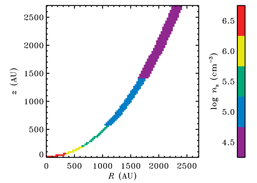
Figure 4: Segmentation of the outflow cavity wall of HH 46 into regions of different pre-shock densities. The cooling length is larger for lower densities, so the shocks are wider at larger radii.

Our method is specifically designed to simulate optically thin emission from shocks. Low-$J$ CO lines typically observed in and associated with outflows, such as the 2–1 and 3–2, originate in cold ($\sim$100 K) swept-up gas present on larger spatial scales than the shocks along the cavity wall (e.g., Arce et al., 2007). These low-$J$ lines are often optically thick and only probe the surface layer of the outflow, where the velocity gradient is largest. Since our focus is on the hot gas observed with Herschel, no attempt is made to quantify the emission from the colder swept-up gas.

An important caveat in the shock models is that they were calculated without a UV field. Several groups are working on irradiated shock models featuring a self-consistent treatment of the UV field in both the pre- and the post-shock gas (e.g., Lesaffre et al. 2011; M. J. Kaufman, priv. comm.), but no such models are currently available. Qualitatively, a UV-irradiated shock is expected to be smaller and hotter, and to have a lower H₂O abundance. The latter is a direct effect of the photodissociation of H₂O. The smaller spatial extent and the higher peak temperature are due to the higher degree of ionization in the irradiated pre-shock gas: the ion-neutral coupling length decreases, so the shock front is compressed and the same amount of energy is imparted over a shorter distance. The shock results are discussed in Sect. 4 with these qualitative arguments in mind.

3 Source sample and observations

The three test cases for the model are the low-mass YSOs NGC1333 IRAS2A, HH 46 IRS and DK Cha (IRAS 12496$-$7650). Each source has been studied extensively in the past, including recent observations with PACS and HIFI on Herschel (van Kempen et al., 2010a, b; Kristensen et al., 2010; Yıldız et al., 2010). The availability of Herschel data and a large body of complementary data is one reason to choose these three sources. Another is that they offer various challenges to the model by spanning a range of evolutionary stages and orientations: IRAS2A is a deeply embedded Stage 0 source seen nearly edge-on (Sandell et al., 1994), HH 46 is a Stage I source seen at a 53^∘ inclination (Nishikawa et al., 2008), and DK Cha is in transition from Stage I to II and is seen nearly pole-on (Knee, 1992). The basic observational characteristics and model parameters for each source are summarised in Table 2.

Far-IR spectra of the three sources were obtained with PACS and HIFI on Herschel (Pilbratt et al., 2010; Poglitsch et al., 2010; de Graauw et al., 2010). The HIFI data used in this work were published by Kristensen et al. (2010) and Yıldız et al. (2010). The PACS spectra of HH 46 and DK Cha were published by van Kempen et al. (2010a, b); the PACS spectrum of IRAS2A is previously unpublished. All PACS data were rereduced with the standard pipeline in HIPE v6.1 (Ott, 2010). A spectral flatfield was applied to the data to improve the signal-to-noise ratio.

PACS consists of a 5$\times$5 integral field unit with $9\aas@@fstack{\prime\prime}4\times 9\aas@@fstack{\prime\prime}4$ spaxels. For HH 46, the fluxes of the central 9$\aas@@fstack{\prime\prime}$4 region are measured directly from the central spaxel and are accurate to 10–20%. The observations of DK Cha and IRAS2A were mispointed by a few arcsec. For both sources, the line emission is concentrated near the location of the continuum emission. In order to measure the line fluxes, the spectra in the four spaxels with the brightest continuum emission were first summed. The ratio of the continuum emission in these four spaxels to the total continuum flux in the $5\times 5$ array was then used to obtain a wavelength-dependent curve to convert the four-spaxel extraction into a flux in the entire field of view. The fluxes were multiplied by the fraction of the flux that falls in the central spaxel (ranging from 70% below 100 $\mu$m to 40% at 200 $\mu$m) to estimate the total flux that would have been in the central spaxel of a well-pointed observation. These corrections assume a point source and may therefore overestimate the flux in the central spaxel. Excluding this uncertainty, the fluxes for IRAS2A and DK Cha are accurate to about 30%. Fluxes and upper limits for all three sources are tabulated in Table 3.

Table 3: Measured line fluxes ($10^{-18}$ W m^-2) from the central region around each source.

Transition	$E_{\rm u}/k$	$\lambda$	IRAS2A	HH 46	DK Cha
	(K)	($\mu$m)
CO
14–13	581	186.00	73	52	207
15–14	663	173.63	112		221
16–15	752	162.81	67	44	219
17–16	846	153.27	64		238
18–17	945	144.78	80	58	245
19–18	1050	137.20	95
20–19	1160	130.37	$<$51
21–20	1276	124.19	$<$94
22–21	1397	118.58	$<$53	35	186
23–22	1524	113.46	177	74	327
24–23	1657	108.76	62	26	200
27–26	2086	96.77	187
28–27	2240	93.35	140
29–28	2400	90.16	$<$35	20	254
30–29	2565	87.19	$<$50	18	147
31–30	2735	84.41	297	74	263
32–31	2911	81.81	$<$33	$<$33	163
33–32	3092	79.36	$<$36	$<$23	92
34–33	3279	77.06	$<$122		234
35–34	3471	74.89	$<$29		209
36–35	3669	72.84	$<$131	$<$24	129
37–36	3872	70.91	$<$33		69
38–37	4080	69.07	$<$25		118
H2O
$2_{21}$–$2_{12}$	194	180.49	77	6	$<$23
$2_{12}$–$1_{01}$	114	179.53	105	7	33
$3_{03}$–$2_{12}$	197	174.62	101	10	89
$3_{22}$–$3_{13}$	297	156.19	109
$3_{13}$–$2_{02}$	205	138.53	105	8	69
$4_{04}$–$3_{13}$	320	125.35	58	4	38
$5_{33}$–$5_{24}$	725	113.95	$<$33	$<$6	$<$31
$\mathit{4_{14}}$–$\mathit{3_{03}}$	3234	113.54	177	74	327
$7_{43}$–$7_{34}$	1340	112.51	34
$2_{21}$–$1_{10}$	194	108.07	237	13	$<$74
$7_{44}$–$7_{35}$	1335	90.05	$<$33	$<$5	$<$63
$3_{22}$–$2_{11}$	297	89.99	97	$<$5	$<$63
$7_{16}$–$7_{07}$	1013	84.77	$<$29	$<$7	$<$45
$6_{06}$–$5_{15}$	643	83.28	182		$<$51
$8_{35}$–$7_{44}$	1511	81.69	$<$28	$<$6	$<$126
$9_{27}$–$9_{18}$	1729	81.40	$<$29	$<$5	$<$125
$4_{23}$–$3_{12}$	432	78.74	38	$<$7	$<$86
$3_{21}$–$2_{12}$	305	75.38	126		$<$87
$9_{37}$–$9_{28}$	1750	73.61	158		$<$126
$8_{18}$–$7_{07}$	1071	63.32	$<$39	$<$11	$<$177

The Herschel data are combined with observations of lower-$J$ CO and CO isotopologue lines (up to 7–6) obtained with the James Clerk Maxwell Telescope (JCMT) and the Atacama Pathfinder Experiment (APEX; Jørgensen et al., 2002; van Kempen et al., 2006, 2009; Yıldız et al., 2010). The different beam sizes for the JCMT, APEX and Herschel are taken into account by convolving the line fluxes from the model with a wavelength-dependent beam size appropriate for the instrument with which each line was observed.

4 Results

4.1 Physical and chemical structure

The best-fit DUSTY envelope model of HH 46 has a radius of 16 100 AU (cut off at 10 K) and a mass of 1.7 $M_{\odot}$ (Table 2). The envelope of NGC1333 IRAS2A is a little smaller (14 100 AU), but because of the shallower density profile its mass comes out 20% higher at 2.0 $M_{\odot}$. DK Cha has the smallest and least massive envelope: 5700 AU and 0.02 $M_{\odot}$. The density and temperature profiles of each envelope are plotted in Fig. 5.

Figure 5: Density and temperature profiles for the passively heated envelopes of the three sources.

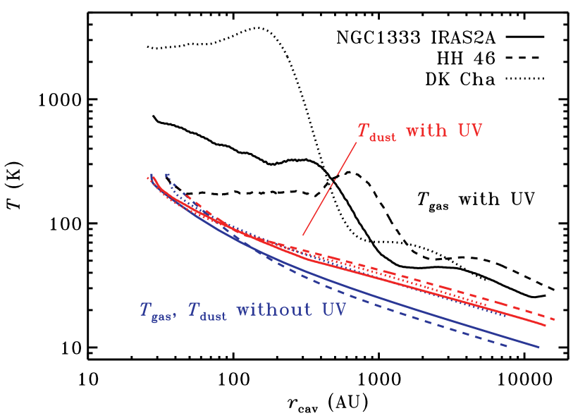
Figure 6: Gas temperature (black) and dust temperature (red) along the cavity wall of the three sources due to UV heating. Shocks are not included. The coordinate on the horizontal axis is the distance to the protostar (Eq. (2)). The blue curves show the temperature profiles due to passive heating only (gas and dust coupled).

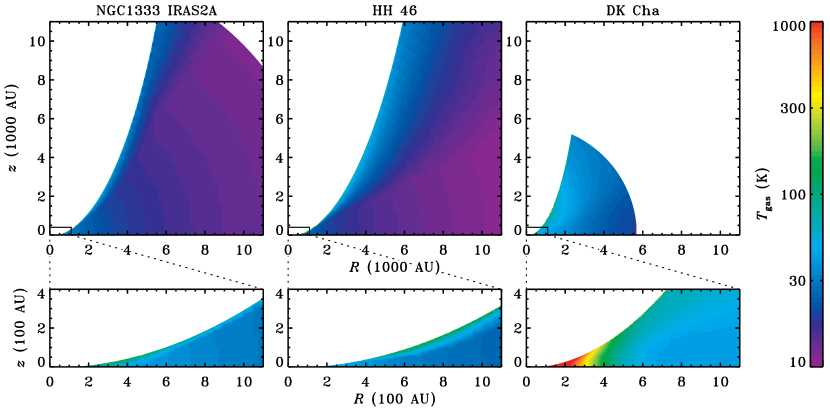
Figure 7: Gas temperature profiles due to UV heating of the outflow cavity walls. Shocks are not included. The bottom row zooms in on the regions indicated in the top row.

When the cavities are carved out of the spherical envelopes, the gas and dust are heated up by the stellar UV flux. The best-fit UV luminosities for the three central sources are determined in Sect. 4.2 by fitting a grid of luminosities to the CO observations. The resulting temperature profiles along the cavity walls are shown in Fig. 6 (black and red curves). For comparison, the plot also shows the temperature profiles from DUSTY (blue), which is what the gas and dust would reach in the absence of UV heating. The effect of UV heating is strongest for DK Cha because of the lower envelope densities. The gas temperature peaks at 3800 K at 150 AU from the star. IRAS2A reaches its maximum of 850 K right at the inner edge, followed by a small secondary maximum of 330 K at 320 AU. For HH 46, the density in the inner envelope is high enough that the gas initially remains coupled to the dust and has the same temperature. At larger distances, the decreasing density allows the gas to become hotter than the dust, reaching a maximum of 260 K at 670 AU.

The full 2D gas temperature profiles in Fig. 7 show that the effects of UV heating are not limited to just the cavity wall, but penetrate some depth into the envelope according to the $\exp(-0.6A_{\rm V})$ depth dependence from Sect. 2.2.1. The thickness of the UV-heated layer ranges from about 100 AU at $r=1000$ AU to about 2000 AU at the outer edge of the envelope. Hence, the UV-heated layer is about a factor of 10 thicker than the shock-heated layer (Fig. 3). Accounting for the predicted effects of the UV field on the shock structure, the thickness ratio between the two layers would be even larger (Sect. 2.3).

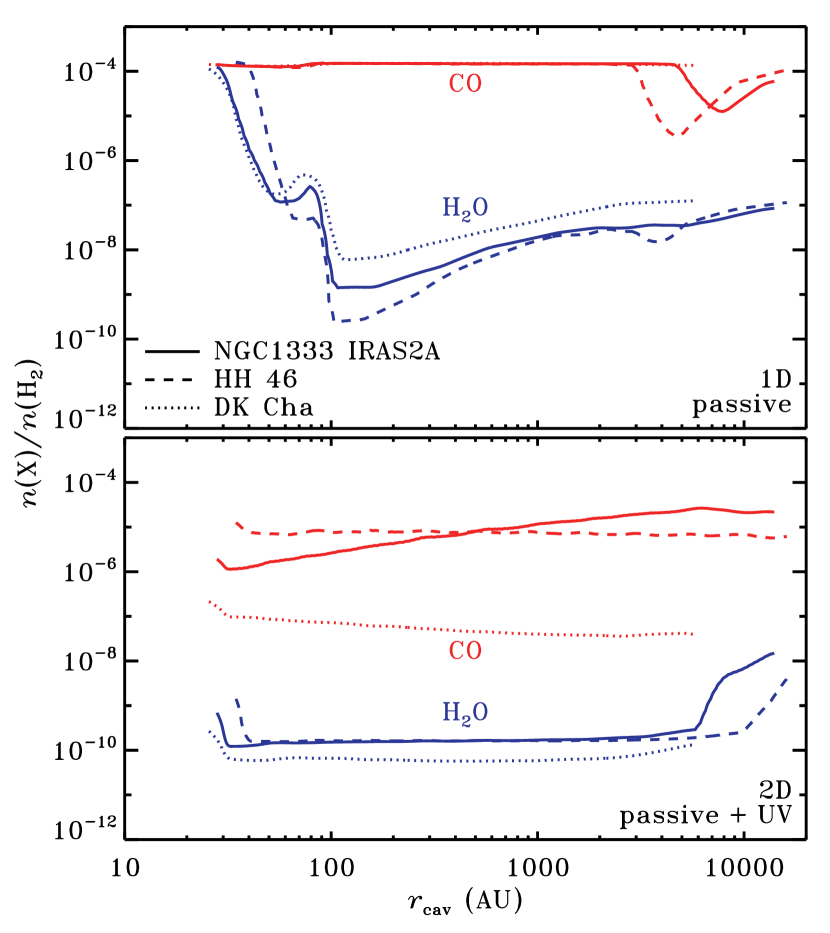
Figure 8: Top: radial abundance profile of CO (red) and H₂O (blue) in the spherical envelope models with passive heating only. Bottom: abundance profiles along the cavity wall (Eq. (2)) in the 2D models, with all effects of the UV field included: photodissociation, photodesorption, and altered chemistry due to heating of the gas and dust. Shocks are not included in either panel.

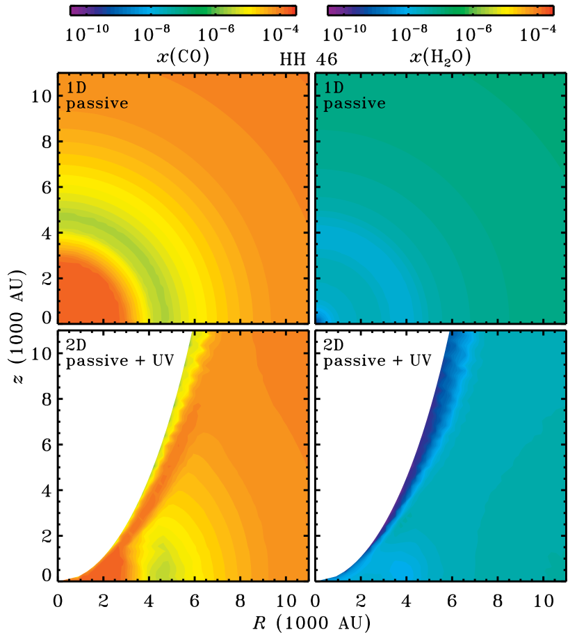
Figure 9: Abundance of CO (left) and H₂O (right) in two versions of the HH 46 model: the spherical envelope with passive heating only (top) and the envelope with UV-heated outflow cavity walls (bottom).

In the purely spherical models for IRAS2A and HH 46, the CO abundance follows a drop profile (top panel of Fig. 8 and top left panel of Fig. 9): it is high ($\sim$$10^{-4}$) in the warm inner parts of the envelope, low ($\sim$$10^{-6}$–$10^{-5}$) at larger radii due to freeze-out onto cold dust, and high again ($\sim$$10^{-4}$) towards the outer edge because of the low density and corresponding long freeze-out timescale (Schöier et al., 2004; Jørgensen et al., 2005; Yıldız et al., 2010). DK Cha has a somewhat warmer envelope (Fig. 5), preventing CO from freezing out and keeping its abundance at $10^{-4}$ at all radii.

There is no freeze-out either along the cavity wall in any of the 2D models (bottom panel of Fig. 8 and bottom left panel of Fig. 9), because the dust temperature now exceeds the CO evaporation temperature everywhere (Fig. 6). The 10 000 K blackbody adopted for the stellar spectra is energetic enough to dissociate some CO in the cavity wall, reducing its abundance to $10^{-6}$–$10^{-5}$ in IRAS2A and HH 46, and $\sim$$10^{-7}$ in DK Cha (Fig. 8, bottom). Moving from the cavity wall towards the midplane, the increasing amount of extinction shields CO from the dissociating photons, and the abundance goes back up to $\sim$$10^{-4}$ (Fig. 9; see Fig. 10 in the online appendix for the other two sources). The dust near the midplanes of HH 46 and IRAS2A remains cold enough for CO to stay frozen, as evidenced by the green region in the bottom left panel of Fig. 9. As a result, horizontal cuts from the cavity wall into the envelope essentially show drop-abundance profiles (Figs. 12 and 13 in the online appendix). CO is not expected to freeze out in the less massive and warmer envelope of DK Cha, so the horizontal cuts merely show the effect of the photodissociation rate decreasing with distance to the cavity wall (Figs. 10 and 14).

10

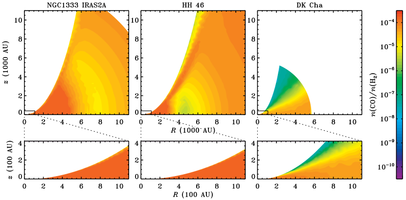
Figure 10: Abundance profiles for CO for the model with outflow cavities and UV heating. Shocks are not included. The bottom row zooms in on the regions indicated in the top row.

The protostellar UV field also dissociates H₂O, making for a nearly uniform abundance of $10^{-10}$ along the wall of each of the three sources (Fig. 8). Moving into the envelope, the increasing amount of extinction slows down the photodissociation process and the H₂O abundance increases to a few $10^{-8}$ in the two regions where it does not freeze out: the warm inner envelope and the low-density outer envelope (Fig. 9, bottom right). In between, freeze-out keeps the abundance limited to at most a few $10^{-9}$. As in the case of CO, the original 1D abundance profiles largely survive at the midplane (Figs. 11–14 in the online appendix).

11

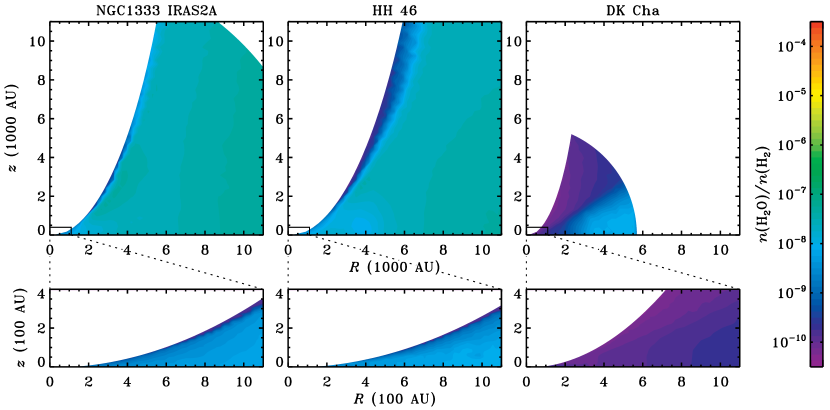
Figure 11: As Fig. 10, but for H₂O.

12

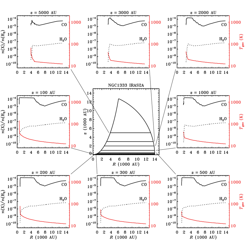
Figure 12: Gas temperature (red) and abundances of CO and H₂O (solid and dotted black) in eight horizontal cuts through the envelope of NGC1333 IRAS2A.

13

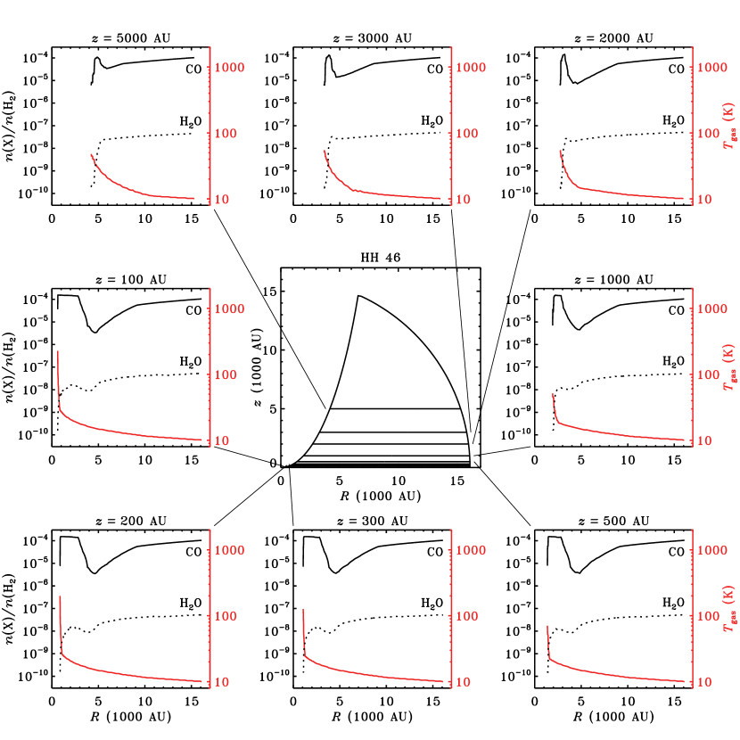
Figure 13: Gas temperature (red) and abundances of CO and H₂O (solid and dotted black) in eight horizontal cuts through the envelope of HH 46.

14

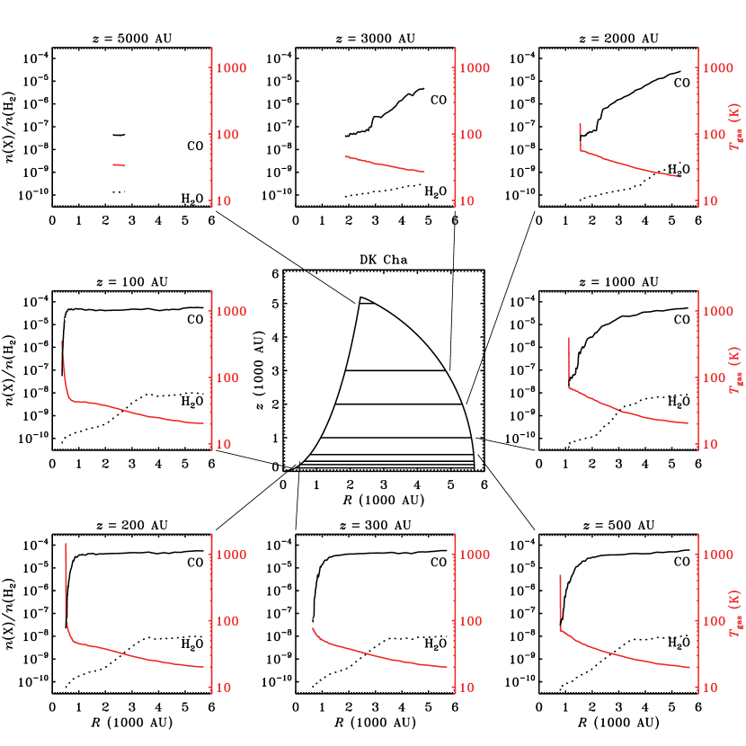
Figure 14: Gas temperature (red) and abundances of CO and H₂O (solid and dotted black) in eight horizontal cuts through the envelope of DK Cha.

With the conditions in the passively heated gas and the UV-heated gas established, the final question is what happens in the small-scale shocks along the cavity walls. As shown in Fig. 3, the peak temperature in a 20 km s^-1 shock ranges from 1300 to 3800 K for pre-shock densities from $10^{4}$ to $10^{6.5}$ cm^-3. In addition, the peak temperature depends roughly linearly on the shock velocity (e.g., Flower & Pineau Des Forêts, 2010). The higher temperatures help overcome the barriers on the ${\rm O}\ +\ {\rm H}_{2}\ \to\ {\rm OH}\ +\ {\rm H}$ and ${\rm OH}\ +\ {\rm H}_{2}\ \to\ {\rm H}_{2}{\rm O}\ +\ {\rm H}$ reactions (Bergin et al., 1998), so the H₂O abundance in the shocked gas is expected to be orders of magnitude higher than the value of $10^{-10}$ calculated for the UV-heated gas (Fig. 8).

The shock models of Flower & Pineau des Forêts (2003) predict a peak H₂O abundance of $\sim$$10^{-4}$ (Fig. 3), but that is in the absence of a UV field (Sect. 2.3). The photodissociation and reformation timescales can be estimated to get an idea of how much the H₂O abundance would change in an irradiated shock. At 1000 AU from the protostar, the UV flux is equivalent to $G_{0}\approx 100$, which gives a photodissociation timescale of about 1 yr (van Dishoeck et al., 2006). A reformation timescale of about 1 yr occurs for $T=1000$ K and $n({\rm H}_{2})=10^{5}$ cm^-3 (Bergin et al., 1998). The density at 1000 AU is closer to $10^{6}$ cm^-3 (Fig. 5), so the reformation timescale is a factor of a few shorter than the photodissociation timescale. However, the two numbers are similar enough that in reality either process could dominate over the other, in particular when considering different points along the cavity wall. A new generation of shock models, incorporating UV radiation, is needed to solve this issue. Until then, the peak H₂O abundance of $\sim$$10^{-4}$ in Fig. 3 should be considered an upper limit only.

4.2 UV luminosities and shock velocities

The model has two free parameters – the UV luminosity and the shock velocity – for which the best-fit values are obtained by comparing the computed CO line fluxes to the available Herschel observations in a $\chi^{2}$ procedure. The lower-$J$ CO lines observed from the ground are not included in the fit. They contain contributions from the parent molecular cloud and from colder swept-up gas, neither of which is present in our model. The H₂O observations are also not used to constrain the model. The grid of UV luminosities runs from 0.01 to 1 $L_{\odot}$. The grid of shock velocities runs from 10 to 35 km s^-1, approximately the critical velocity of C-type shocks for the relevant density regime (Sect. 2.3).

As an example of the dynamic range of the free parameters, Fig. 15 shows the predicted line fluxes for HH 46 for a range of values. The top panel shows how the combined flux from the passively heated envelope and the UV-heated outflow cavity walls changes as function of UV luminosity. The bottom panel does so for the flux from the small-scale shocks as function of shock velocity. These figures are qualitatively the same for the other two sources.

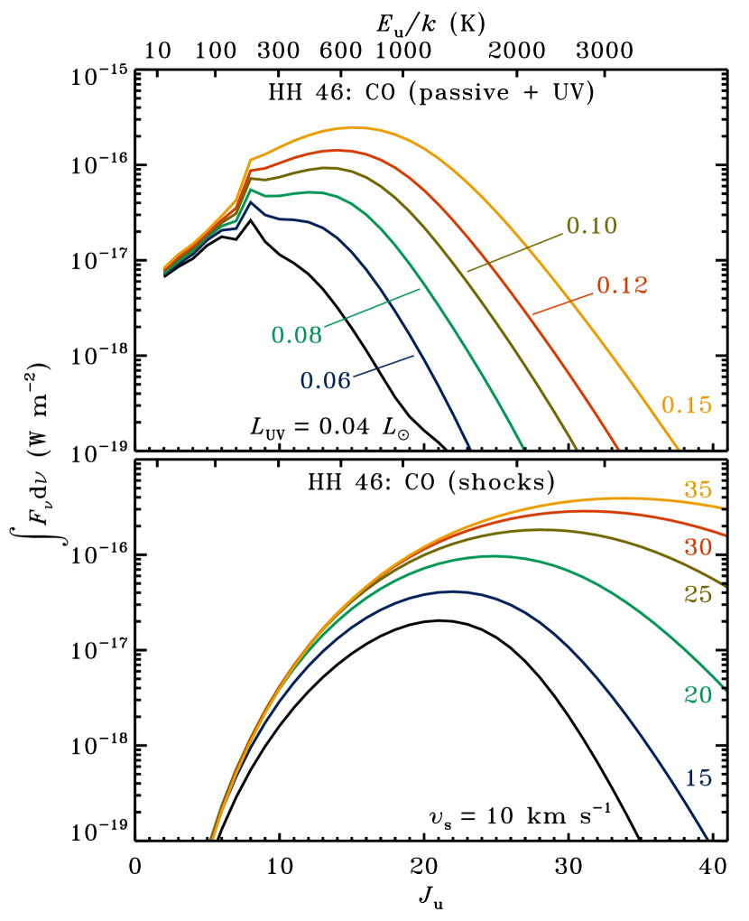
Figure 15: Top: CO fluxes computed for the passive and UV components in HH 46 together, for UV luminosities ranging from 0.06 to 0.15 $L_{\odot}$. Bottom: CO fluxes computed for the shock component in HH 46, for shock velocities ranging from 10 to 35 km s^-1.

The best-fit UV luminosities and shock velocities are tabulated in Table 2 and shown in Fig. 16. Overplotted in the figure are the 1, 2 and $3\sigma$ confidence intervals. Both parameters are well constrained in HH 46. In IRAS2A, the UV luminosity is only constrained from the top. In DK Cha, the shock velocity is unconstrained at the 3$\sigma$ level and only constrained from below at the 2$\sigma$ level. Extending the grid of luminosities to lower values does not resolve the issue for IRAS2A, because the gas cannot cool below the dust temperature. The $\chi^{2}$ analysis suggests that the CO fluxes observed with Herschel are powered primarily by shocks in IRAS2A, by UV-heating in DK Cha, and by a combination of both in HH 46. This result is discussed in more detail in the next section.

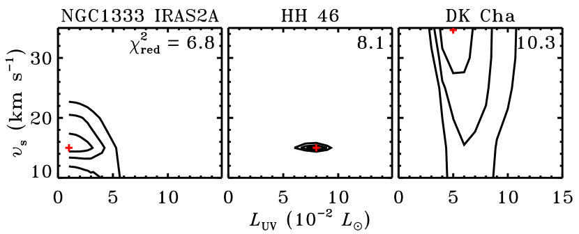
Figure 16: Reduced $\chi^{2}$ contours for the UV luminosity and the shock velocity in each source. Red crosses mark the minima. Contours are at the 1, 2 and $3\sigma$ levels.

4.3 Line fluxes

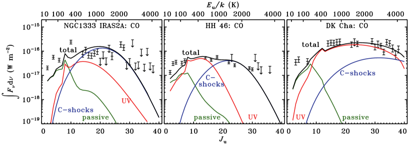
Figure 17: CO line fluxes observed with the JCMT, APEX and Herschel. Overplotted are the fluxes from the three model components (green, red and blue) and their sums (black). Error bars (1$\sigma$) reflect the 10–30% calibration uncertainty of Herschel and the 20–30% calibration uncertainty of the JCMT and APEX. Upper limits are at the $3\sigma$ level.

4.3.1 Carbon monoxide

With the physical and chemical structure from Sect. 4.1 and the best-fit UV luminosities and shock velocities from Sect. 4.2 (taking $L_{\rm UV}=0.01$ $L_{\odot}$ for IRAS2A and $\varv_{\rm s}=35$ km s^-1 for DK Cha), the model produces the integrated CO line fluxes shown in Fig. 17. Also plotted are the integrated line fluxes observed from the ground and with Herschel. The only systematic discrepancy between model and observations is an underproduction of the 2–1, 3–2 and 4–3 lines. The same discrepancy was seen by van Kempen et al. (2009) in their purely spherical model of HH 46. The excess flux probably originates in cold gas in the parent molecular cloud or in cold swept-up outflow gas, neither of which is included in our model. The low-$J$ lines of the less abundant C¹⁸O isotopologue are not expected to have any significant cloud or outflow contribution (e.g., Jørgensen et al., 2002; Yıldız et al., 2010), and indeed the model reproduces the available C¹⁸O data to within 50%. The mismatches with some of the individual Herschel data points in Fig. 17 do not appear to follow any systematic trend. They are likely due to uncertainties in the model fluxes and minor factors such as pointing offsets and calibration uncertainties that may be larger than the estimated 10–30%.

The coloured curves in Fig. 17 show the predicted contribution from the passively heated envelope (green), the UV-heated cavity walls (red) and the small-scale shocks (blue) to the total CO emission (black). Each source requires a combination of UV-heated gas and small-scale shocks to reproduce the Herschel data, although there are clear qualitative differences from source to source. IRAS2A is the youngest of the three sources (deeply embedded Stage 0) and its CO ladder appears to be dominated by shock-powered emission. HH 46 is more evolved (Stage I) and shows a 50/50 split between UV-powered and shock-powered emission. DK Cha is still more evolved (in transition from Stage I to II) and its small-scale shocks are responsible for only a small fraction of the overall CO emission. The decreasing contribution of the shock component is consistent with the general trend of the outflow force being weaker in more evolved protostars (Bontemps et al., 1996). The increasing contribution of the UV component is powered by the decreasing densities in the envelope, allowing the gas to become hotter (Figs. 5 and 6; see also Sect. 5.1). Although the sample size is small, the observed data are entirely in keeping with these physically motivated trends. Application of the model to a larger number of sources, such as the full WISH sample, will help to obtain a firmer conclusion. Furthermore, a full parameter study is planned to assess systematically how the CO emission depends on properties such as the envelope mass and the UV luminosity.

Table 4: Absolute and relative luminosities of CO and H₂O for the three physical components in each source.

Component	IRAS2A		HH 46		DK Cha
for CO	$10^{-3}$ $L_{\odot}$	%	$10^{-3}$ $L_{\odot}$	%	$10^{-3}$ $L_{\odot}$	%
passive	0.3	7	0.5	7	0.1	2
UV	0.8	20	3.1	45	4.0	78
C-shocks	3.0	73	3.3	48	1.0	20
total	4.1	100	6.9	100	5.1	100
Component	IRAS2A		HH 46		DK Cha
for H2O	$10^{-3}$ $L_{\odot}$	%	$10^{-3}$ $L_{\odot}$	%	$10^{-3}$ $L_{\odot}$	%
passive	0.02	0.02	0.53	0.38	0.05	0.17
UV	0.001	0.001	0.04	0.03	$3(-5)$	$1(-4)$
C-shocks	100	$>$99.9	140	99.6	30	99.8
total	100	100	140	100	30	100

The contribution in each curve can be quantified by summing the line fluxes from $J_{\rm u}=2$ to 40 and correcting them for distance to give the overall CO luminosities for the adopted inclinations (Table 4). The CO line fluxes can also be plotted in a rotational diagram to investigate excitation conditions. Table 5 lists the rotational temperatures derived by fitting straight lines to the passive curve from $E_{\rm u}=10$ to 100 K (up to $J=5$–4), to the UV curve from 100 to 1000 K (up to $J=18$–17), and to the shock curve from 1000 to 4000 K. The error margins reflect the stochastic $1\sigma$ uncertainty on each fit, but do not account for any uncertainties in the model results.

Table 5: Rotational temperatures for CO and H₂O in the three physical components in each source.

Component	IRAS2A	HH 46	DK Cha
for CO	$T_{\rm rot}$ (K)	$T_{\rm rot}$ (K)	$T_{\rm rot}$ (K)
passive	$31\pm 5$	$33\pm 9$	$54\pm 5$
UV	$240\pm 30$	$160\pm 20$	$410\pm 100$
C-shocks	$380\pm 20$	$400\pm 20$	$1600\pm 50$
Component	IRAS2A	HH 46	DK Cha
for H2O	$T_{\rm rot}$ (K)	$T_{\rm rot}$ (K)	$T_{\rm rot}$ (K)
passive	$72\pm 1$	$130\pm 5$	$175\pm 10$
UV	$30\pm 1$	$69\pm 1$	$114\pm 1$
C-shocks	$410\pm 80$	$540\pm 170$	$750\pm 400$

The CO ladder for DK Cha in Fig. 17 implies that the six CO lines seen with ISO, from $J=14$–13 to 19–18 (Giannini et al., 1999), originate in the UV-heated gas in the outflow cavity walls. Based on a passively heated spherical envelope model, van Kempen et al. (2006) concluded that the ISO lines trace material on larger spatial scales than the material responsible for the 7–6 and lower lines observed with APEX. With the more complex source geometry in our model, such a requirement no longer exists. In fact, the temperature gradient along the cavity wall (Fig. 6), together with the pole-on inclination, suggests the high-$J$ lines seen with ISO originate on smaller spatial scales than the lower-$J$ APEX lines. A more detailed analysis of the spatial extent of the PACS data, using all $5\times 5$ spaxels, can help to solve the puzzle, but this is beyond the scope of the current work.

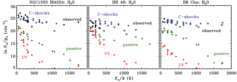
Figure 18: Rotational diagrams for water. Black: Herschel detections (circles) and $3\sigma$ upper limits (triangles). Green, red and blue: model predictions for the passive, UV and shock components.

4.3.2 Water

Figure 18 shows the observations and model predictions for H₂O. The complicated rotational structure of H₂O does not allow for plots in the format of the CO ladders in Fig. 17, so the results are shown as rotational diagrams instead. The individual line fluxes can be summed again to obtain the total line luminosities. However, the models only calculate fluxes for a subset of all possible rotational lines. Fluxes for the missing lines in the HIFI and PACS wavelength ranges (up to $E_{\rm u}/k=2000$ K) are calculated by fitting a single rotational temperature to the available lines in each model component (Table 5). The level populations of H₂O are not in LTE, so this method may produce large errors in the flux of a given individual line. However, because those errors tend to cancel when summing over all possible lines, assuming a single temperature is appropriate for calculating the total line luminosities (see also Goldsmith & Langer, 1999). The resulting values are tabulated in Table 4.

Unlike CO, the H₂O emission observed with Herschel seems to be dominated ($>$99%) by shock-heating in all three sources. This is consistent with the broad H₂O line profiles seen with HIFI in IRAS2A and other embedded YSOs (Kristensen et al. 2010, subm.). Our shock models actually overproduce many of the detections and upper limits by up to a factor of 10, in particular in HH 46 (Fig. 18). The likely cause is that the H₂O abundances in our shock models were calculated without taking the protostellar UV field into account. Based on the photodissociation and reformation timescales estimated in Sect. 4.1, the H₂O abundance can easily be lowered by a factor of 2 to 10 from the peak value of $10^{-4}$ shown in Fig. 3. At the same time, the abundance of OH would go up, so our shock models are currently expected to underproduce the OH line intensities. However, as argued by van Kempen et al. (2010b) and Wampfler et al. (2010), the OH lines observed with Herschel likely originate in a different physical component than the H₂O lines (a dissociative J-type shock instead of a non-dissociative C-type shock). It is therefore not possible to test whether the OH line intensities predicted for the small-scale shocks are indeed lower than the actual OH emission from that component. A potential problem with lowering the H₂O abundances through photodissociation is that some CO in the shock may be dissociated as well. If that happens, a higher shock velocity is required to fit the CO observations, which in turn would raise the model H₂O fluxes back to their original values of up to an order of magnitude too high. An independent constraint on the CO and H₂O abundances in UV-irradiated shocks is needed to fully resolve this issue.

Another difference between CO and H₂O is seen in the relative contributions of the passive and UV components. For H₂O, both are weak compared to the shock-powered emission, but the passive component is always the brighter of the two (Table 4). The weak emission from the UV-heated gas in the outflow cavity walls is due to the very low H₂O abundance (Figs. 8 and 9), which in turn is due to the wide range of photon energies over which H₂O can be dissociated. CO can only be dissociated by photons of at least 11 eV, so its abundance in the cavity walls remains higher and the UV-heated gas contributes a larger fraction of the overall CO emission.

5 Discussion

5.1 Gas temperature

The largest unknown in our model is the gas temperature due to UV heating of the outflow cavity walls. Calculating the gas and dust temperatures for a given density and UV flux is a standard problem in models of photon-dominated regions (PDRs; e.g., Tielens & Hollenbach, 1985; Hollenbach & Tielens, 1997). However, the PDR community has not yet converged on a unique solution: in a benchmark test of ten different PDR codes, the temperature solutions varied by up to an order of magnitude (Röllig et al., 2007). As shown in Sect. 4.3, the temperature grid from Kaufman et al. (1999, hereafter K99), along with the $\exp(-0.6A_{\rm V})$ depth dependence derived from the benchmark test, works well to reproduce the CO observations. However, given the complicated nature of our model, this does not necessarily mean that the K99 grid gives the correct temperatures. For example, if the grid systematically overpredicts the temperature, it may still give a good match to the data by decreasing the UV luminosity. Other temperature grids may also be able to match the data. The goal of this section is two-fold: (1) to show that, at least on a qualitative level, the K99 grid follows the density and UV flux dependence expected from basic heating and cooling physics for the relevant range of conditions; and (2) to see how robust our results are to changes in the adopted temperature grid.

The K99 grid is reproduced in Fig. 19. In its original form, it only covers H₂ densities up to $10^{7}$ cm^-3. The densities in our model go up to $10^{9}$ cm^-3, so the grid is extrapolated as $T_{\rm gas}\propto 1/n({\rm H}_{2})$. The $n^{-1}$ dependence comes from the approximate functional forms of the heating and cooling mechanisms expected to dominate at high densities: photoelectric heating ($\propto n$; Bakes & Tielens, 1994) and gas-grain collisional cooling ($\propto n^{2}$; Hollenbach & McKee, 1989). The density dependence of the temperature in the original K99 grid is almost exactly $n^{-1}$ between $10^{6}$ and $10^{7}$ cm^-3.

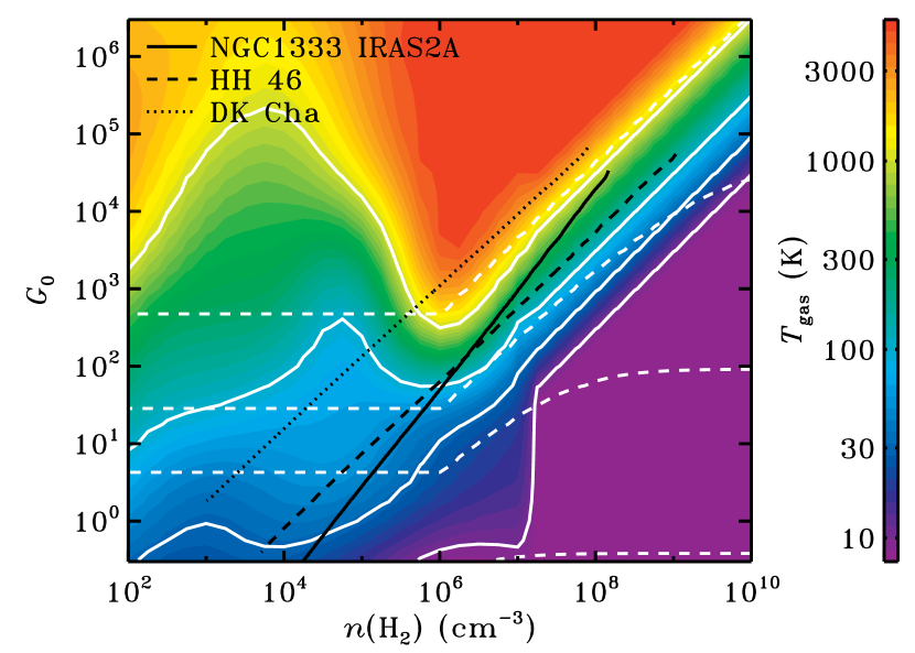
Figure 19: PDR surface temperature grid (colour scale and solid white contours) from Kaufman et al. (1999), extrapolated as $T_{\rm gas}\propto n^{-1}$ for $n({\rm H}_{2})>10^{7}$ cm^-3. The white contours are drawn at 10, 30, 100 and 1000 K. Overplotted as dashed white contours (same values) is the approximate temperature grid based on Eqs. (5.1) and (7). The black lines trace the conditions along the cavity walls of the three sources.

Overplotted as black lines in Fig. 19 are the gas density and incident UV flux along the cavity walls of the three sources. The density and UV flux both fall off approximately as $r^{-2}$, so they scale linearly with each other. At densities above $\sim$$10^{6}$ cm^-3, the gas temperature is expected to scale with the inverse of the density (see above) and linearly with the UV flux (Bakes & Tielens, 1994), and should therefore remain constant along the inner part of the wall. This is indeed seen in Fig. 6: $T_{\rm gas}$ does not change much over the range of radii corresponding to densities of more than $10^{6}$ cm^-3. Photoelectric heating likely remains dominant at lower densities, but atomic fine-structure lines take over from gas-grain collisions as the dominant cooling mechanism. Their cooling rate depends linearly on the density as long as the density exceeds the critical density of $3\times 10^{3}$ cm^-3 for the [C ii] 158 $\mu$m line, so the temperature is expected to remain roughly constant with density (K99; Meijerink et al., 2007). Because the $G_{0}$ dependence remains, the temperature along the cavity wall should decrease as $r^{-1}$ for $n({\rm H}_{2})<10^{6}$ cm^-3. Again, this is the approximate behaviour seen in Fig. 6. The dependencies change again for densities below $3\times 10^{3}$ cm^-3, but such low densities do not appear in our model.

The location of the black lines in Fig. 19 shows why the UV-powered CO emission looks qualitatively different in DK Cha than in IRAS2A and HH 46. The lower envelope densities in the former turn the conditions along the cavity wall into a classic PDR, with densities of $10^{6}$–$10^{7}$ cm^-3 and UV fluxes of $10^{3}$–$10^{4}$ times the mean interstellar flux. The gas therefore gets much hotter and CO is excited to higher rotational levels. The steep temperature gradient in this part of Fig. 19 also means that the CO emission is rather sensitive to details in the SED fitting with DUSTY. A factor of two difference in density leads to a similar change in the gas temperature, which can affect the highest-$J$ CO lines by a few orders of magnitude. Figure 17 tentatively shows an evolutionary trend of the CO emission in more evolved sources being more strongly UV-powered. While the application of a physical model is necessary to quantify exactly how much of the total CO ladder in a given source is due to UV heating, the observations are consistent with the main point that with decreasing density (assuming sufficient UV), sources becomes more PDR-like. This is what one would naturally expect in the transition from Stage 0 to Stages I and II objects as presented in this paper.

Of equal importance to the CO emission is the choice of the PDR temperature grid. An easy way to get a rough idea of how changes in the adopted grid would affect the CO line fluxes is to parameterise the gas temperature based on the dominant heating and cooling mechanisms. Two equations suffice to do so. The first one approximates the gas-grain collisional cooling rate (Hollenbach & McKee, 1989):

$$\Lambda_{\rm g-g}=\ (1\times 10^{-31}\,{\rm erg}\,{\rm cm}^{-3}\,{\rm s}^{-1})n_{\rm H}^{2}\sqrt{\frac{T_{\rm gas}}{1000\,{\rm K}}}\sqrt{\frac{100\,\text{\AA}}{a_{\rm min}}}$$

$$\left[1-0.8\exp\left(-\frac{75\,{\rm K}}{T_{\rm gas}}\right)\right](T_{\rm gas}-T_{\rm dust})\,,$$ (6)

where $n_{\rm H}$ is the total hydrogen nucleus density (equal to $2n({\rm H}_{2})$ in our model for all practical purposes) and $a_{\rm min}$ is the minimum grain size (set to 10 Å). The second equation is for the photoelectric heating rate (Bakes & Tielens, 1994):

$$\Gamma_{\rm pe}=(1\times 10^{-24}\,{\rm erg}\,{\rm cm}^{-3}\,{\rm s}^{-1})\epsilon G_{0}n_{\rm H}\,.$$ (7)

The photoelectric heating efficiency, $\epsilon$, is treated as a free parameter for the purpose of this simple approximation. As such, it hides any uncertainties in the grain charge and in the numerical prefactors in the two equations (see, e.g., Young et al., 2004). Given a dust temperature from RADMC (or, alternatively, from the analytical expression of Hollenbach et al. 1991), the gas temperature at $n({\rm H}_{2})>10^{6}$ cm^-3 is obtained by solving for $\Lambda_{\rm g-g}=\Gamma_{\rm pe}$. At lower densities, the dependence of $T_{\rm gas}$ on $n({\rm H}_{2})$ disappears to zeroth order, and we set $T_{\rm gas}[G_{0},n({\rm H}_{2})<10^{6}\ {\rm cm}^{3}]=T_{\rm gas}[G_{0},10^{6}\ {\rm cm}^{3}]$.

Figure 19 shows the 10, 30, 100 and 1000 K contours for $\epsilon=0.2$ as dashed white lines. The approximate grid reproduces the K99 grid to within a factor of 2 for the full range of densities and UV fluxes encountered along the three cavity walls. The approximation breaks down for $G_{0}/n({\rm H}_{2})<10^{-4}$ (high density, low UV) and $G_{0}/n({\rm H}_{2})>10^{-3}$ (low density, high UV), and cannot be used in either of those regimes. The value of 0.2 required for a good match with K99 exceeds the maximum value of 0.05 allowed by Bakes & Tielens (1994). However, the approximate temperature grid is purely meant as an easy tool to study the effect of different temperature grids, so this factor of 4 should not be considered physically important. The key point is that the K99 grid and the approximate grid show the same qualitative trends for the relevant range of conditions, which means the K99 grid follows the behaviour expected from the dominant heating and cooling mechanisms.

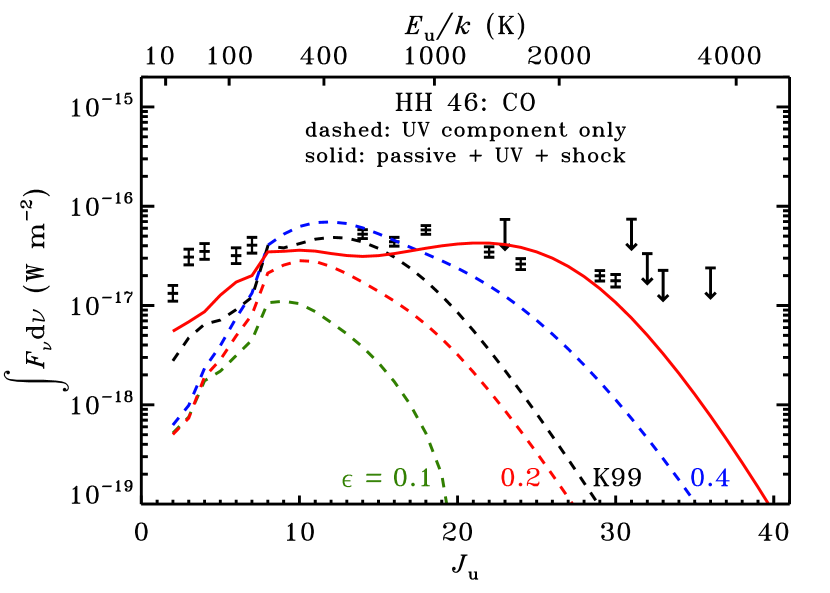
Figure 20: CO ladder for HH 46. The data points are as in Fig. 17. The dashed black curve is the model flux for the UV component for temperatures from the Kaufman et al. (1999) grid. The dashed coloured curves are the same, but for the temperature approximation from Eqs. (5.1) and (7), using different heating efficiencies. The solid red curve combines the dashed red curve with the passive and shock curves from Fig. 17.

With $\epsilon=0.2$, the approximate grid does a good job of reproducing the CO line emission for the UV component. Shown in Fig. 20 are the integrated line fluxes from the UV-heated gas in HH 46, using either the K99 grid (dashed black curve, identical to the red curve from Fig. 17) or the approximate grid with three different values of $\epsilon$ (dashed coloured curves). The $\epsilon=0.2$ curve lies within 30% of the K99 curve up to $J_{\rm u}=20$, at which point shocks take over as the dominant producer of CO emission. When adding the passive and shock components to the $\epsilon=0.2$ curve (producing the solid red curve), the overall agreement with the data is as good as in Fig. 17. Taking a lower or higher photoelectric heating efficiency would under- or overproduce the $J=14$–13, 16–15 and 18–17 lines.

The photoelectric heating rate scales linearly with $\epsilon$ and $G_{0}$ (Eq. (7)), so the three values of $\epsilon$ in Fig. 20 can be brought to give the same CO fluxes by changing the UV luminosity. Herein lies the degeneracy alluded to at the beginning of this section and in Sect. 4.2: as long as two temperature grids show the same qualitative trends, both can reproduce the CO observations, but they have different best-fit UV luminosities. This degeneracy can only be lifted by calibrating the temperature grids against a source whose incident UV flux can be constrained independently in the same part of $n({\rm H}_{2})$–$G_{0}$ parameter space.

5.2 Caveats in the shock models

The shock modelling relies on three assumptions: (1) the shocks move along the cavity walls, (2) the effective beam-filling factor can be obtained from accurately estimating the shock width, and (3) the protostellar UV field does not affect the H₂O abundance. In order to test where the emission is coming from in this scenario – extended lower-density gas with a large beam-filling factor or higher-density gas with a small beam-filling factor – fluxes from the standard shock model are compared to fluxes from models without any contribution from gas with densities of $10^{4}$ cm^-3 and lower, $10^{5}$ cm^-3 and lower, or $10^{6}$ cm^-3 and lower. The shock velocity is kept at 20 km s^-1 for this experiment. For the case of HH 46, gas at densities below $10^{4}$ cm^-3 is found to contribute less than $10^{-4}$%, and gas at densities between $10^{4}$ and $10^{5}$ cm^-3 only 0.3%. About 75% of the overall flux comes from the segment with a pre-shock density of $10^{6.5}$ cm^-3. The other two sources show almost the same numbers, indicating that the shocked gas observed by PACS is dominated by emission from the densest parts of the YSO.

If the density is assumed to be fixed at more than $10^{6}$ cm^-3, the shock velocity alone determines the absolute line fluxes. This was already seen in the bottom panel of Fig. 15, where the basic shape of the CO ladder is nearly independent of velocity. Hence, the velocity determines the intensity of the CO emission, and the pre-shock density determines the shape of the ladder. Comparing the fluxes amongst the three sources, the differences are dominated by their respective distances. This confirms that the actual geometry only plays a small role with respect to the predicted CO emission, and that the bulk of emission is created in very dense gas contained within the central PACS spaxel.

If the effective beam-filling factor is treated as a free parameter, it becomes degenerate with the shock velocity. A smaller beam-filling factor would require a higher shock velocity to produce the same line fluxes, and vice versa. However, for a given source geometry, such as the ellipsoid outflow cavity in our model, the beam-filling factor follows from the cooling lengths and is not truly a free parameter. The only way to constrain either the geometry or the beam-filling factor would be to have an independent handle on the pre-shock density and the shock velocity. Our method therefore gives a unique solution for the given shock geometry, but other geometries cannot be excluded.

6 Conclusions

The Herschel Space Observatory offers a new probe into the hot gas present in embedded low-mass young stellar objects (YSOs) through emission lines of highly rotationally excited CO (up to 4000 K above the ground state) and H₂O (up to 600 K). This paper presents the first model to reproduce these observations quantitatively. The model starts with a passively heated spherical envelope, which fits the lowest-$J$ CO isotopologue lines observed from the ground, but falls short of the ¹²CO Herschel data by several orders of magnitude. Two additional model components are therefore invoked: (1) gas in the walls of a bipolar outflow cavity, exposed to the protostellar UV field, and (2) small-scale C-type shocks along the cavity walls.

The main conclusion is that, within the context of the model, the far-infrared CO rotational line emission in the low-mass YSOs NGC1333 IRAS2A, HH 46 and DK Cha can only be reproduced with a combination of UV-heated gas and C-type shocks. The three sources show a tentative evolutionary trend: the CO emission appears to be dominated by shock-heating in the youngest source (IRAS2A), by UV-heating in the oldest source (DK Cha), and by a 50/50 combination in the source of intermediate age (HH 46). This trend is powered by the envelope density decreasing as a protostar evolves from Stage 0 to Stages I and II.

The H₂O lines are dominated by shocks in all three sources, with less than 1% of the total H₂O line luminosity originating in UV- and passively heated gas. This is a direct result of the different abundances in the three components. Freeze-out keeps the H₂O abundance below $10^{-8}$ in the cold outer envelope. The dust grains in the UV-heated layer are warm enough for H₂O to evaporate, but it is dissociated by the UV field once it does. Efficient reformation at high temperatures boosts the abundance to $10^{-5}$–$10^{-4}$ in the C-type shocks, so they are responsible for most of the H₂O emission. CO has a lower evaporation temperature (20 versus 100 K), so its abundance is orders of magnitude higher than that of H₂O in the passively heated and the UV-heated gas, allowing these two components to contribute more strongly to the overall CO emission.

The main uncertainty in the model lies in the calculation of the gas temperature as function of the incident UV flux. This is a well-known problem in photon-dominated regions (PDRs), and many solutions are available in the literature. However, they disagree by up to an order of magnitude and some do not even agree qualitatively on how the gas temperature depends on the density or the UV flux. The sensitivity of our model results to the treatment of the gas temperature is tested with an approximate analytical description of the expected dominant heating and cooling mechanisms. This exercise shows that the quantitative contributions of the UV-heated gas and the C-type shocks to the hot gas emission observed by Herschel are uncertain by at least a factor of 2, but the qualitative conclusion that both components are needed to explain the observations is robust.