Bridge Copula Model for Option Pricing

Abstract

In this paper we present a new multi-asset pricing model, which is built upon newly developed families of solvable multi-parameter single-asset diffusions with a nonlinear smile-shaped volatility and an affine drift. Our multi-asset pricing model arises by employing copula methods. In particular, all discounted single-asset price processes are modeled as martingale diffusions under a risk-neutral measure. The price processes are so-called UOU diffusions and they are each generated by combining a variable (Itô) transformation with a measure change performed on an underlying Ornstein-Uhlenbeck (Gaussian) process. Consequently, we exploit the use of a normal bridge copula for coupling the single-asset dynamics while reducing the distribution of the multi-asset price process to a multivariate normal distribution. Such an approach allows us to simulate multidimensional price paths in a precise and fast manner and hence to price path-dependent financial derivatives such as Asian-style and Bermudan options using the Monte Carlo method. We also demonstrate how to successfully calibrate our multi-asset pricing model by fitting respective equity option and asset market prices to the single-asset models and their return correlations (i.e. the copula function) using the least-square and maximum-likelihood estimation methods.

Introduction

Many quantitative finance applications require a multi-asset pricing model with dependencies between the single-asset price components. Compared to the variety of univariate asset price models, the pool of multi-asset pricing models is not so extensive. Most of multivariate models are based on multidimensional geometric Brownian motion with the possible inclusion of a jump process. In this paper we develop and explore a new multi-asset arbitrage-free pricing model based on a special family of nonlinear diffusions. The development of efficient computational methods for pricing multi-asset equity derivatives under such a model and the calibration of the multi-asset model to both standard equity option data as well as historical equity prices are the objectives of the current paper.

Here, we specialize on option pricing applications under so-called UOU diffusion models, which are obtained by transforming an underlying Ornstein-Uhlenbeck diffusion process via the use of a diffusion canonical transformation method (see [2, 3, 5, 8] and references therein). For all choices of model parameters, all discounted (single-asset) price processes UOU are conservative martingales under a risk-neutral measure. Since the univariate diffusions are solvable, the single-asset risk-neutral transition probability density function is given in analytically closed form. Moreover, implied volatility surfaces for this highly nonlinear asset price model exhibit a wide range of pronounced smiles and skews of the type observed in the option markets. The main relevant features of the univariate UOU model are summarized in Section 1.

To construct a multivariate probability distribution, one can use a copula function that allows us to couple univariate distribution functions. Sampling from the obtained joint multivariate distribution function thereby reduces to sampling from the copula function and from the univariate distributions. Therefore, the copula method allows us to construct the joint distribution and density functions as well as to obtain an exact path sampling algorithm.

The main computational disadvantage of such an approach is the calculation of inverses of the distribution functions. This operation can be a rather time-consuming computational problem for a complicated multi-parameter distribution. Nevertheless, such a drawback can be significantly improved if the copula function and univariate distributions have a similar structure. As is shown in Subsection 1.3, the bridge probability density function (conditional on the values of the process at the endpoints of a time interval) of a UOU diffusion is reduced to a normal density. Hence it is natural to couple univariate UOU bridges using a Gaussian copula. Based on this idea, in Section 2, we construct a two-step algorithm for the exact path simulation of the multidimensional (nonlinear) UOU process in the risk-neutral measure. Firstly, we apply a usual copula method for sampling the multi-asset process at the terminal (maturity) time. Secondly, we use a bridge sampling along with a multivariate normal distribution to model the process at any intermediate time.

In Section 3, we demonstrate the calibration of the univariate and multivariate models to historical asset and equity option prices. The calibration process has two stages. First, we calibrate all univariate (marginal) asset price models independently of each other. Using the least-square method the models can be fitted to standard European option prices. Alternatively, the maximum likelihood estimation (MLE) allows the models to be fitted to historical asset prices. Second, we fit the copula function to historical observations. Since, our model assumes a normal copula, we need to find a best-fitted normal correlation matrix.

In Section 4, we give computational applications of the model to pricing multi-asset path-dependent Asian-style and Bermudan options. In pricing Bermudan options we use a regression-based Monte Carlo method.

In summary, the main results of our paper include: the construction a new family of multivariate models for which marginal processes are local volatility smile diffusions; the development of calibration schemes for the single-asset and multi-asset pricing UOU diffusion models based on the least-square and MLE methods; the construction of an exact multivariate path simulation method that can be used for Monte Carlo pricing of generally path-dependent European-style and American-style options.

1 Ornstein-Uhlenbeck Family of Univariate State-Dependent Volatility Diffusion Models

1.1 Diffusion Canonical Transformation

The diffusion canonical transformation method, first presented in [2] and then further developed in [15, 5, 8], leads to various families of solvable one-dimensional diffusions with a nonlinear diffusion coefficient function and an affine drift. In this paper, we consider the $\mathsf{UOU}$ family, which is based on a regular Ornstein-Uhlenbeck process $(X_{t})_{t\geq 0}\in\mathcal{I}\equiv\mathds{R}$. The regular Ornstein-Uhlenbeck process is defined by the infinitesimal generator

$$\mathcal{L}f(x)\equiv\frac{1}{2}\nu^{2}f^{\prime\prime}(x)-\lambda xf^{\prime}(x)\,,\;\;x\in\mathds{R},$$ (1.1)

where $\lambda>0$ and $\nu>0$ are constants. Both left and right boundaries $l=-\infty$ and $r=\infty$ of the state space $\mathcal{I}$ are non-attracting natural for all choices of parameters. The transition probability density function (PDF) is

$$p_{X}(t;x_{0},x)=\sqrt{\frac{\kappa}{2\pi(1-e^{-2\lambda t})}}\exp\left(-\frac{\kappa(x-x_{0}e^{-\lambda t})^{2}}{2(1-e^{-2\lambda t})}\right)\,,$$ (1.2)

where we define $\kappa\equiv\frac{2\lambda}{\nu^{2}}>0$.

Let $\rho>0$ be a strictly positive constant. Then, two fundamental solutions of $\mathcal{L}\varphi(x)=s\varphi(x)$, $x\in\mathcal{I}$, are given by

$$\varphi^{-}_{\rho}(x)=\exp\left(\frac{\kappa x^{2}}{4}\right)D_{-\upsilon}(x\sqrt{\kappa})\quad\mbox{and}\quad\varphi^{+}_{\rho}(x)=\varphi^{-}_{\rho}(-x),$$ (1.3)

where $\upsilon\equiv\rho/\lambda>0$ and $D_{-\upsilon}(\cdot)$ is Whittaker’s parabolic cylinder function (see [1]). The solutions $\varphi^{+}_{\rho}(x)$ and $\varphi^{-}_{\rho}(x)$ are linearly independent and respectively increasing and decreasing positive functions of $x\in\mathds{R}$.

We now construct another diffusion process $(S_{t})_{t\geq 0}\in\mathcal{D}=\mathds{R}_{+}=(0,\infty)$ by applying a diffusion canonical transformation to the underlying Ornstein-Uhlenbeck diffusion. This process obeys the stochastic differential equation (SDE)

$$\mathrm{d}S_{t}=rS_{t}\mathrm{d}t+\sigma(S_{t})\mathrm{d}W_{t},\,\,S_{t=0}=S_{0}\,,$$ (1.4)

where $r$ is a constant and $\sigma(S)$ is a nonlinear diffusion coefficient function. Here $({W}_{t})_{t\geq 0}$ is a standard Brownian motion in some appropriate probability measure ${\mathds{P}}$.

The initial step of the transformation is to apply a Doob’s $h$-transform or $\rho$-excessive transform (see [4]) to $(X_{t})$. The resulting diffusion process $\big{(}X^{(\rho)}_{t}\big{)}_{t\geq 0}$ is defined by the following infinitesimal generator:

$$\mathcal{L}^{(\rho)}f(x)=\frac{1}{2}\nu^{2}f^{\prime\prime}(x)+\lambda_{\rho}(x)f^{\prime}(x),\;x\in\mathcal{I},$$ (1.5)

where $\lambda_{\rho}(x)\equiv-\lambda x+\nu^{2}\hat{u}_{\rho}^{\prime}(x)/\hat{u}_{\rho}(x)$ for any $\rho>0$. The strictly positive generating function is given by $\hat{u}_{\rho}(x)=q_{1}\varphi^{+}_{\rho}(x)+q_{2}\varphi^{-}_{\rho}(x)$ with parameters $q_{1},q_{2}\geq 0,$ $q_{1}+q_{2}>0$. The process $(X^{(\rho)}_{t})$ has the transition PDF

$$p_{X}^{(\rho)}(t;x_{0},x)=e^{-\rho t}\frac{\hat{u}_{\rho}(x)}{\hat{u}_{\rho}(x_{0})}p_{X}\left(t;x_{0},x\right),\;x,x_{0}\in\mathcal{I},\,t>0.$$ (1.6)

The final step of the transformation is a change of variable (see [8] for a more general discussion). We define a new process $S_{t}=\mathsf{F}(X_{t}^{(\rho)})$, $t\geq 0$, that solves SDE (1.4) by finding a strictly monotonic map that solves $\mathcal{L}^{(\rho)}\mathsf{F}(x)=r\mathsf{F}(x)$, for constant $r$. Then $\sigma(\mathsf{F}(x))=\nu|\mathsf{F}^{\prime}(x)|$ or equivalently $\sigma(s)=\nu/|\mathsf{X}^{\prime}(s)|$, where $\mathsf{X}\equiv\mathsf{F}^{-1}$ defines the unique inverse map. The transition PDF $p_{S}$ for the process $(S_{t})$ follows from that for the underlying process $(X_{t})$:

$$p_{S}(t;s_{0},s)=\frac{\nu}{\sigma(s)}\;p_{X}^{(\rho)}(t;x_{0},x)=\frac{\nu}{\sigma(s)}\frac{\hat{u}_{\rho}(x)}{\hat{u}_{\rho}(x_{0})}e^{-\rho t}p_{X}\left(t;x_{0},x\right),$$ (1.7)

$x=\mathsf{X}(s)$, $x_{0}=\mathsf{X}(s_{0})$.

We now apply the above construction to a subfamily of diffusions with choice $q_{1}=0,q_{2}=1$, i.e. with generating function $\hat{u}_{\rho}(x)=\varphi^{-}_{\rho}(x)$. Letting $r+\rho>0$ and $\rho>0$, we specifically consider

$$\mathsf{F}(x)=c\frac{\varphi^{+}_{r+\rho}(x)}{\varphi^{-}_{\rho}(x)}=c\frac{D_{-\upsilon-r/\lambda}(-x\sqrt{\kappa})}{D_{-\upsilon}(x\sqrt{\kappa})}\,.$$ (1.8)

This function maps $x\in\mathds{R}$ onto $s\in(0,\infty)$ and is monotonically increasing, where $s=\mathsf{F}(x)$ has the unique inverse relation $x=\mathsf{X}(s)$. This transformation leads to a family of diffusions $(S_{t})$ that is referred to as the unbounded Ornstein-Uhlenbeck ($\mathsf{UOU}$) family with the diffusion coefficient function given by

$$\sigma(s)=\nu\sqrt{\kappa}e^{\frac{\kappa x^{2}}{4}}\left((\upsilon+\frac{r}{\lambda})\frac{D_{-\upsilon-1-\frac{r}{\lambda}}(-\sqrt{\kappa}x)}{D_{-\upsilon}(\sqrt{\kappa}x)}+\upsilon\frac{D_{-\upsilon-\frac{r}{\lambda}}(-\sqrt{\kappa}x)}{D_{-\upsilon}(\sqrt{\kappa}x)}\frac{D_{-\upsilon-1}(-\sqrt{\kappa}x)}{D_{-\upsilon}(\sqrt{\kappa}x)}\right),$$ (1.9)

where $x=\mathsf{X}(s)$. The volatility function $\sigma$ in (1.9) depends on several adjustable positive parameters such as $c,\nu,\lambda,\rho$, and more generally $r\neq 0$ also enters as an additional parameter within the volatility specification. Notice that for the driftless case with $r=0$ formula (1.9) simplifies as follows: $\sigma(\mathsf{F}(x))=\displaystyle\frac{\sigma_{0}\mathfrak{s}(x)}{\hat{u}_{\rho}^{2}(x)},$ where $\sigma_{0}>0$ is a constant and $\mathfrak{s}(x)=e^{\frac{\kappa x^{2}}{2}}$ is the scale density for the $X$-diffusion.

The following is an important statement for the purposes of risk-neutral pricing.

Lemma 1.1 ([8]).

Consider a process $(S_{t})_{t\geq 0}\in\mathds{R}_{+}$ of the UOU family solving the SDE (1.4) with the diffusion coefficient $\sigma$ specified by (1.9) and having transition PDF $p_{S}$ specified by equations (1.7), (1.8), (1.9) and given by

$$p_{S}(t;s_{0},s)=\frac{e^{-\rho t+\kappa(x^{2}-x_{0}^{2})/4}}{c\mathcal{W}(x)}\frac{D_{-\upsilon}^{\,3}(x\sqrt{\kappa})}{D_{-\upsilon}(x_{0}\sqrt{\kappa})}p_{X}(t;x_{0},x),\quad t>0,\;s,s_{0}>0,$$ (1.10)

where $\mathcal{W}(x)=W[D_{-\upsilon}(x\sqrt{\kappa}),D_{-\upsilon-r/\lambda}(-x\sqrt{\kappa})]>0$ is the Wronskian, and $x=\mathsf{X}(s)$, $x_{0}=\mathsf{X}(s_{0})$. Then $(S_{t})$ is a conservative process, i.e. $\mathds{P}(S_{t}\in\mathds{R}_{+})=1$ for all $t>0$. Moreover, the discounted asset price process $(e^{-rt}S_{t})_{t\geq 0}$ is a true martingale.

1.2 Pricing Vanilla Options

According to Lemma 1.1 there exists an equivalent martingale measure under the UOU family with transition PDF (1.10) for any choice of the model parameters. Consider a standard European-style option defined by its payoff function $\Lambda(S)$ at terminal price $S=S_{T}$ and maturity (expiration) time $T>t_{0}=0$. For example, a vanilla European call has the payoff function $C^{E}(S)=(S-K)^{+}\equiv\max\{S-K,0\},$ where $K>0$ is a strike price. The valuation of a standard European option is given by the conditional expectation under a risk-neutral probability measure $\mathds{P}\equiv\mathds{Q}$:

$$V(S_{0},T)=e^{-rT}\mathds{E}^{\mathds{Q}}[\Lambda(S_{T})\mid S_{t=0}=S_{0}]=e^{-rT}\mathds{E}^{\mathds{Q}}[\Lambda(\mathsf{F}(X_{T}^{(\rho)}))\mid X_{0}^{(\rho)}=x_{0}]\,.$$ (1.11)

This is reduced to the valuation of a one-dimensional integral expressible as follows:

$$\begin{array}[]{rcl}V(S_{0},T)&=&e^{-rT}\displaystyle\int_{0}^{\infty}p_{S}(T;S_{0},s)\Lambda(s)\;\mathrm{d}s\\[10.0pt] &=&\displaystyle\frac{e^{-(r+\rho)T}}{\hat{u}_{\rho}(x_{0})}\int_{-\infty}^{\infty}\hat{u}_{\rho}(x)\,p_{X}(T;x_{0},x)\Lambda(\mathsf{F}(x))\,\mathrm{d}x\,,\end{array}$$ (1.12)

where $x_{0}=\mathsf{X}(S_{0}).$

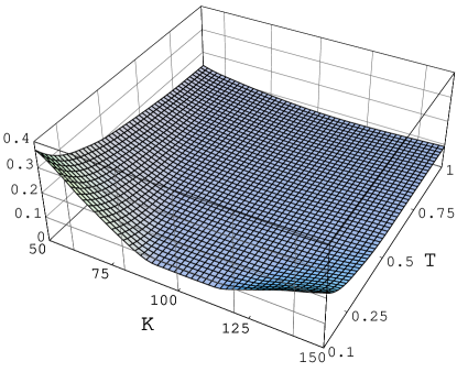
Figure 1: Local volatility (or log-normal volatility) function $\sigma(S)/S$ (left plot) and Black-Scholes impled volatility surface (right plot) for the $\mathsf{UOU}$ family. The $\mathsf{UOU}$ family is plotted using model parameters $c=100$; $\rho=0.005$, $\kappa=5$, $\upsilon=0.1$ (thin line) and $\rho=0.02$, $\kappa=1$, $\upsilon=0.5$ (thick line). The implied volatility surface, with $T$ as time to maturity and $K$ as strike price, corresponds to the same choice of parameters as the local volatility plot drawn with the thin line. The interest rate $r=0.1$ and spot $S_{0}=100$ are used.

1.3 The UOU Bridge

Let us consider a bridge process on $[t_{1},t_{2}]$, $0\leq t_{1}<t_{2}$, generated by a single asset price process $S_{t}$ with $S_{t_{1}}$ and $S_{t_{2}}$ fixed at $s_{1}$ and $s_{2}$, respectively. The bridge density $b_{S}(t;s)\equiv b_{S}(t_{1},t_{2},t;s_{1},s_{2},s)$ for $S_{t}=s$, $t_{1}<t<t_{2}$, conditional on $S_{t_{1}}=s_{1}$ and $S_{t_{2}}=s_{2}$, is given by

$$\begin{split}&b_{S}(t;s)\equiv\displaystyle\frac{p_{S}(t-t_{1};s_{1},s)\,p_{S}(t_{2}-t;s,s_{2})}{p_{S}(t_{2}-t_{1};s_{1},s_{2})}\\[11.38109pt] \mbox{}&=\displaystyle\frac{\nu}{\sigma(s)}\,\frac{p_{X}^{(\rho)}(t-t_{1};x_{1},\mathsf{X}(s))\,p_{X}^{(\rho)}(t_{2}-t;\mathsf{X}(s),x_{2})}{p_{X}^{(\rho)}(t_{2}-t_{1};x_{1},x_{2})}\\[14.22636pt] \mbox{}&=\displaystyle\frac{\nu}{\sigma(s)}\,\frac{p_{X}(t-t_{1};x_{1},\mathsf{X}(s))\,p_{X}(t_{2}-t;\mathsf{X}(s),x_{2})}{p_{X}(t_{2}-t_{1};x_{1},x_{2})}\equiv\displaystyle\frac{\nu}{\sigma(s)}b_{X}(t;\mathsf{X}(s)),\end{split}$$ (1.13)

where $x_{1}\equiv\mathsf{X}(s_{1})$, $x_{2}\equiv\mathsf{X}(s_{2})$, and $b_{X}(t;x)\equiv b_{X}(t_{1},t_{2},t;x_{1},x_{2},x)$ is the bridge PDF of the underlying $X$-diffusion conditional on the endpoint values $X_{t_{1}}=x_{1}$ and $X_{t_{2}}=x_{2}$. Since the underlying process $(X_{t})$ is a Gaussian process, the bridge process, generated by $(S_{t})_{t\geq 0}$, with transition PDF (1.13) is just a nonlinear transformation of a Gaussian bridge, with respective path points mapped as $X_{t}=\mathsf{X}(S_{t})$. Thus, the bridge PDF $b_{S}$ for $(S_{t})$ from the UOU family can be reduced to a Gaussian PDF for the underlying $X$-process. Indeed, from Eq. (1.2) we see that the bridge PDF $b_{X}$ of the Ornstein-Uhlenbeck diffusion is a normal density $\varphi(x)=\frac{1}{\sqrt{2\pi}b}e^{-(x-\mu)^{2}/2b^{2}}$ with mean $\mu$ and variance $b^{2}$ given by

$$\begin{array}[]{rcl}\mu&=&\displaystyle\frac{x_{1}e^{\lambda\Delta_{1}}(e^{2\lambda\Delta_{2}}-1)+x_{2}e^{\lambda\Delta_{2}}(e^{2\lambda\Delta_{1}}-1)}{e^{2\lambda(\Delta_{1}+\Delta_{2})}-1},\\[10.0pt] b^{2}&=&\displaystyle\frac{(e^{2\lambda\Delta_{1}}-1)(e^{2\lambda\Delta_{2}}-1)}{\kappa(e^{2\lambda(\Delta_{1}+\Delta_{2})}-1)},\end{array}$$ (1.14)

where $\Delta_{1}\equiv t-t_{1},$ $\Delta_{2}\equiv t_{2}-t$, and $\Delta_{1}+\Delta_{2}=t_{2}-t_{1}$.

2 Multivariate UOU-Diffusion Pricing Model

2.1 Coupling UOU Processes

Our goal is to construct a multi-asset price process $(\mathbf{S}_{t})_{t\geq 0}$ with $\mathbf{S}_{t}\equiv\left(S_{t}^{1},\ldots,S_{t}^{n}\right)$, where each individual asset price process $(S_{t}^{k})_{t\geq 0}$, $k=1,2,\ldots,n,$ is a univariate UOU diffusion obeying (1.4) with common drift parameter $r$ and diffusion function $\sigma=\sigma^{k}$. Suppose that each of the $n$ univariate processes is described by its own set of positive parameters $\xi_{k}=\left\{\lambda_{k},\nu_{k},c_{k},\rho_{k}\right\},$ $k=1,2,\ldots,n.$ We denote by $p^{k}_{S}$ and $\sigma^{k}$ the univariate risk-neutral transition PDF of the form (1.10) and the diffusion coefficient given by (1.9), respectively, which both correspond to the $k$-th asset price process. In the following, for each $k=1,2,\ldots,n$, $\hat{u}^{k}_{\rho_{k}}$, $\mathsf{F}^{k}$, and $\mathsf{X}^{k}$ will respectively denote the generating function, the mapping function, the inverse mapping function of the $k$th diffusion model. The transition PDFs $p^{k}_{X}$ and $p_{X}^{(\rho_{k},k)}$ correspond to the underlying diffusion $(X^{k}_{t})_{t\geq 0}$ and the transformed diffusion $\left(X_{t}^{(\rho_{k},k)}\right)_{t\geq 0}$, respectively. All the above functions indexed by $k$ are obtained by using the parameters from $\xi_{k}$ in the respective equations provided in Section 1.

Recall that the processes $(S^{k}_{t})_{t\geq 0}$, $k=1,2,\ldots,n$, are defined by the transformation $\mathsf{F}^{k}$ given by (1.8), i.e. $S^{k}_{t}=\mathsf{F}^{k}(X_{t}^{(\rho_{k},k)})$ where $(X_{t}^{(\rho_{k},k)})_{t\geq 0}$ are defined by (1.5) with $\lambda=\lambda_{k}$, $\nu=\nu_{k}$, and $\rho=\rho_{k}$. For an infinitesimal time increment $\delta t$, consider $\delta S^{k}_{t}\equiv S^{k}_{t+\delta t}-S^{k}_{t}$ and $\delta X_{t}^{(\rho_{k},k)}\equiv X_{t+\delta t}^{(\rho_{k},k)}-X_{t}^{(\rho_{k},k)}$. It follows that $\delta S^{k}_{t}\simeq(\mathsf{F}^{k})^{\prime}(X_{t}^{(\rho_{k},k)})\cdot\delta X_{t}^{(\rho_{k},k)}$. From the map, $(\mathsf{F}^{k})^{\prime}(x)=\sigma^{k}(\mathsf{F}^{k}(x))/\nu_{k}$, we readily see that the respective correlations between the ratios of the infinitesimal increment and the diffusion coefficient remain the same after the change of variables:

$$\mathrm{corr\,}\left(\frac{\delta S_{t}^{k}}{\sigma^{k}(S_{t}^{k})},\frac{\delta S_{t}^{\ell}}{\sigma^{\ell}(S_{t}^{\ell})}\right)\simeq\mathrm{corr\,}\left(\frac{\delta X_{t}^{(\rho_{k},k)}}{\nu_{k}},\frac{\delta X_{t}^{(\rho_{\ell},\ell)}}{\nu_{\ell}}\right),\quad k,\ell=1,\ldots,n.$$ (2.1)

This relation shows how to couple UOU diffusions. First of all, we can directly couple the processes $\left(X_{t}^{(\rho_{k},k)}\right)$, which, in turn, introduces correlations among the asset price processes $(S^{k}_{t})$. In fact, the same method is used to couple geometric Brownian motions that are just exponentially transformed Brownian motions with drift. Hence, by using dependent Brownian motions, one introduces the correlations between the log-returns. In the case of more general diffusions, one may introduce correlations between the volatility-scaled returns. Alternatively, one may couple the underlying $X$-processes. For example, it is possible to use a multivariate Ornstein-Uhlenbeck process as an underlying vector process. Another approach (which is not discussed in this paper) is to extend the diffusion canonical transformation method directly to the case of multivariate diffusion processes.

Another idea, and the one that we implement in this paper, is the coupling of $X^{(\rho)}$-bridges. As is shown in Subsection 1.3, the bridge PDF of a UOU $X^{(\rho)}$-process is the same as the density function of the Ornstein-Uhlenbeck bridge, which is a multivariate normal PDF. The respective multivariate distribution function obtained with the use of a Gaussian copula is nothing more than a multivariate normal CDF. Therefore, the coupling of $X^{(\rho)}$-bridges considerably simplifies the form of the joint path distribution function as well as the path simulation algorithm.

2.2 Copula Function

A copula $\mathcal{C}(u_{1},u_{2},\ldots,u_{n})$ is a multivariate cumulative distribution function (CDF) defined on the $n$-dimensional unit cube $[0,1]^{n}$ such that every marginal distribution is uniform on the unit interval $[0,1]$ (for a more detailed definition we refer to [16]). Suppose that $\Phi^{1},\Phi^{2},\ldots,\Phi^{n}$ are univariate distribution functions, e.g., $\Phi^{k}(x)=\int_{-\infty}^{x}f^{k}(y)\,\mathrm{d}y$, where $f^{k}$ is a respective univariate PDF. It follows that $\mathcal{C}(\Phi^{1}(x_{1}),\ldots,\Phi^{n}(x_{n}))$ is a multivariate CDF with marginals $\Phi^{k}(x)=\mathcal{C}(1,\ldots,1,u_{k}=\Phi^{k}(x),1,\ldots,1),$ $k=1,2,\ldots,n$. The well-known Sklar’s theorem states that any $n$-dimensional joint distribution function $\mathbf{\Phi}$ with continuous marginals $\Phi^{1},\ldots,\Phi^{n}$ has a unique copula representation:

$$\mathbf{\Phi}(x_{1},x_{2},\ldots,x_{n})=\mathcal{C}(\Phi^{1}(x_{1}),\Phi^{2}(x_{2}),\ldots,\Phi^{n}(x_{n})).$$ (2.2)

In other words, for continuous multivariate distributions, the marginal distributions and the multivariate dependence structure can be separated. The multivariate density function $\mathbf{f}$ is then obtained by differentiating Eq. (2.2):

$$\mathbf{f}(x_{1},\ldots,x_{n})=\frac{\partial^{n}\mathcal{C}(\Phi^{1}(x_{1}),\ldots,\Phi^{n}(x_{n}))}{\partial u_{1}\ldots\partial u_{n}}f^{1}(x_{1})\ldots f^{n}(x_{n}).$$ (2.3)

As a corollary of Sklar’s theorem we have a class of copula functions constructed from continuous multivariate probability distributions as follows:

$$\mathcal{C}(u_{1},u_{2},\ldots,u_{n})=\mathbf{\Phi}\left((\Phi^{1})^{-1}(u_{1}),(\Phi^{2})^{-1}(u_{2}),\ldots,(\Phi^{n})^{-1}(u_{n})\right)\,,$$ (2.4)

for any $(u_{1},u_{2},\ldots,u_{n})\in[0,1]^{n}$, where $(\Phi^{k})^{-1}$ is the inverse of $\Phi^{k}$.

The Gaussian (or normal) copula is one of the most important in financial applications. This copula is constructed from the multivariate normal distribution:

$$\mathcal{C}^{Gauss}_{R}(u_{1},u_{2},\ldots,u_{n})=\mathcal{N}_{R}\left(\mathcal{N}^{-1}(u_{1}),\mathcal{N}^{-1}(u_{2}),\ldots,\mathcal{N}^{-1}(u_{n})\right)\,,$$ (2.5)

where $\mathcal{N}_{R}$ is the standard $n$-variate normal CDF with mean vector zero, unit variances, and correlation matrix $R$. Here, $\mathcal{N}^{-1}$ stands for the inverse of a standard univariate Gaussian CDF.

Consider the problem of sampling from a multivariate distribution given by (2.2). The modelling algorithm consists of two steps. First, we simulate a uniformly distributed vector $(U_{1},U_{2},\ldots,U_{n})\in[0,1]^{n}$ from the copula $\mathcal{C}$. After that, we sample a vector $(X_{1},X_{2},\ldots,X_{n})$ from the marginal distributions by evaluating the inverse CDFs: $X_{k}=(\Phi^{k})^{-1}(U_{k}),$ $k=1,2,\ldots,n$. As is seen, the crucial part of this algorithm is the efficient computation of the inverse of a distribution function.

2.3 Multivariate Path Copula

The objective of this subsection is the derivation of a multivariate path distribution function in closed form. Such a function allows us to obtain an exact path simulation method and also to construct the joint path density function, which is used for calibrating the model with the maximum likelihood estimation method.

We employ the copula method to construct the joint distribution function of the multivariate process $\mathbf{X}_{t}^{(\boldsymbol{\rho})}=\big{(}X_{t}^{(\rho_{1},1)},\ldots,X_{t}^{(\rho_{n},n)}\big{)}.$ The multi-asset price process $\mathbf{S}_{t}=\big{(}S_{t}^{1},\ldots S_{t}^{n}\big{)}$ is then obtained by applying the respective mapping function to each univariate $X^{(\rho)}$-diffusion: $S_{t}^{k}=\mathsf{F}^{k}\left(X_{t}^{(\rho_{k},k)}\right)$, $k=1,2,\ldots,n$.

Suppose that the process $(\mathbf{X}_{t}^{(\boldsymbol{\rho})})$ conditional on $\mathbf{X}_{0}^{(\boldsymbol{\rho})}$ is to be sampled at a set of times $\mathbf{T}=\{t_{j}\}_{j=1}^{N}\in[0,T]$, $T>0$, so that $0=t_{0}<t_{1}<t_{2}<\cdots<t_{N}=T$. Let $\widetilde{\mathbf{T}}=\{\tilde{t}_{j}\}_{j=1}^{N}$ represent some arrangement of time points in $\mathbf{T}$. The ordering of the time points is determined by the simulation method used. For the (forward) sequential method we assume that $0<\tilde{t}_{1}<\cdots<\tilde{t}_{N}=T$, i.e. $\forall j\geq 0\;\tilde{t}_{j}=t_{j}$. For the backward-in-time bridge method we have that $0<\tilde{t}_{N}<\tilde{t}_{N-1}<\cdots<\tilde{t}_{2}<\tilde{t}_{1}=T$, i.e. $\forall j\geq 1\;\tilde{t}_{j}=t_{N+1-j}$. In other words, we first obtain the value of the process at the terminal time $T$ and then simulate a bridge path conditionally on the previously sampled value and the initial value. Notice that for the bridge sampling method, the ordering of intermediate time points $\tilde{t}_{2},\ldots,\tilde{t}_{N}$ may vary, e.g. one can use a forward bridge sampling with $0<\tilde{t}_{2}<\tilde{t}_{3}<\cdots<\tilde{t}_{N}<\tilde{t}_{1}=T$ or a full bridge sampling method, where we successively halve the time interval or its largest segment to sample the process at the midpoint of the time segment conditionally on the previously sampled values at the endpoints of the current time (sub-)interval. The full bridge sampling may be applied along with the quasi-Monte Carlo method.

Let $f^{k}_{j}(x)$ denote the PDF of $X_{\tilde{t}_{j}}^{(\rho_{k},k)}$ conditional on the $\sigma$-algebra $\mathcal{F}^{k}_{j-1}$ generated by the previously sampled $j$ path points $X_{0}^{(\rho_{k},k)},X_{\tilde{t}_{1}}^{(\rho_{k},k)},\ldots,X_{\tilde{t}_{j-1}}^{(\rho_{k},k)}$, where $1\leq j\leq N$ and $1\leq k\leq n$. For the sequential path sampling method, with $\tilde{t}_{i}=t_{i}$, we have that $f^{k}_{j}(x)=p_{X}^{(\rho_{k},k)}\left(t_{j}-t_{j-1};X_{t_{j-1}}^{(\rho_{k},k)},x\right).$

For the backward bridge method we have that $f^{k}_{1}(x)=p_{X}^{(\rho_{k},k)}\left(T;X_{0}^{(\rho_{k},k)},x\right)$. Since all univariate processes are Markovian and are sampled backward in time, for each $j=2,3,\ldots,N$, $f^{k}_{j}(x)$ is a bridge PDF $b_{X}^{k}\left(\tilde{t}_{j};x\right)$ of the Ornstein-Uhlenbeck bridge conditional on $X_{0}^{(\rho_{k},k)}$ and $X_{\tilde{t}_{j-1}}^{(\rho_{k},k)}$, where $\tilde{t}_{j}=t_{N+1-j}$ and $\tilde{t}_{j-1}=t_{N+2-j}$. As is shown in Subsection 1.3, the PDF $b_{X}^{k}$ is a normal density function with mean $\mu_{kj}$ and variance $b^{2}_{kj}$, with values given by (1.14) where $\lambda=\lambda_{k},$ $\kappa=\kappa_{k}$, $\Delta_{1}=\tilde{t}_{j}-t_{0}=\tilde{t}_{j},$ and $\Delta_{2}=\tilde{t}_{j-1}-\tilde{t}_{j}.$

In $X$-space, the joint CDF $\mathbf{\Phi}_{j}$ and respective joint PDF $\mathbf{f}_{j}$ of the $n$-dimensional point $\mathbf{X}_{\tilde{t}_{j}}^{(\boldsymbol{\rho})}$, $j=1,2,\ldots,N$, are then constructed by employing equations (2.2) and (2.3), respectively, where the marginal distribution functions are $\Phi^{k}_{j}(x)=\int_{-\infty}^{x}f^{k}_{j}(x^{\prime})\;\mathrm{d}x^{\prime}$, $k=1,2,\ldots,n$, $j=1,2,\ldots,N$, $x\in\mathds{R}$, $t>0$. Notice that, for the backward-in-time bridge method, the CDF $\Phi^{k}_{j}(x)$ is a normal CDF $\mathcal{N}\left(\frac{x-\mu_{kj}}{b_{kj}}\right)$, for each $j=2,\ldots,N$.

From the Markov property of process $(\mathbf{X}_{t}^{(\boldsymbol{\rho})})$, the multivariate path distribution function $\mathbb{\Phi}$ and the respective joint path density function $\mathbb{f}$ of $\left(\mathbf{X}^{(\boldsymbol{\rho})}_{\tilde{t}_{j}}\right)_{j=1,\ldots,N}$ conditional on $\mathbf{X}^{(\boldsymbol{\rho})}_{0}$ are given by the respective products

$$\mathbb{\Phi}(\mathbf{x}_{1},\ldots,\mathbf{x}_{N})=\prod_{j=1}^{N}\mathbf{\Phi}_{j}(\mathbf{x}_{j})\text{ \ and \ }\mathbb{f}(\mathbf{x}_{1},\ldots,\mathbf{x}_{N})=\prod_{j=1}^{N}\mathbf{f}_{j}(\mathbf{x}_{j}),$$ (2.6)

where $\mathbf{x}_{j}\equiv(x_{j}^{1},\ldots,x_{j}^{n}),$ $j=1,2\ldots,N$. In $S$-space, the joint path PDF $\mathbb{f}^{s}$ and the joint PDFs $\mathbf{f}^{s}_{j}$ of $\mathbf{S}_{\tilde{t}_{j}}$, $j=1,2\ldots,N$, are respectively given by

$$\mathbb{f}^{s}(\mathbf{s}_{1},\ldots,\mathbf{s}_{N})=\prod_{j=1}^{N}\mathbf{f}^{s}_{j}(\mathbf{s}_{j}),\quad\mathbf{f}^{s}_{j}(\mathbf{s}_{j})=\prod_{k=1}^{n}\frac{\nu_{k}}{\sigma^{k}(s^{k}_{j})}f_{j}^{k}\left(\mathsf{X}^{k}(s_{j}^{k})\right),$$ (2.7)

where $\mathbf{s}_{j}=(s_{j}^{1},\ldots,s_{j}^{n})$

To sample from the distribution function in (2.6) we need a fast and accurate algorithm for inverting univariate CDFs. Usually, for non-standard distributions such as the PDF given by formula (1.10), such algorithms are quite computationally intensive. Therefore, the sequential approach becomes rather unfeasible for the path simulation of the multi-asset price UOU process $(\mathbf{S}_{t})$.

As was mentioned above, we apply the Gaussian copula method to construct the underlying vector process $\mathbf{X}_{t}^{(\boldsymbol{\rho})}$ with transition PDFs of the form (1.6) instead of direct coupling of the $S$-space asset price processes. This is then followed by applying a nonlinear transformation to obtain the asset prices $S^{k}_{t}=\mathsf{F}^{k}(X_{t}^{(\rho_{k},k)})$.

To minimize the number of numerical inversions of CDFs, we employ a bridge simulation approach, which is followed by the coupling of the bridge distributions. The application of the Gaussian copula to bridge PDFs from the $\mathsf{UOU}$ diffusion family leads to a multivariate normal distribution. Indeed, if each CDF $\Phi^{k}$ (say, the CDF of the $k$th $X^{(\rho)}$-bridge) is a normal CDF $\mathcal{N}\left(\frac{x-\mu_{k}}{b_{k}}\right)$, then the multivariate CDF $\mathbf{\Phi}$ given by (2.2) with the Gaussian copula in (2.5) is just a multivariate normal distribution function $\mathcal{N}_{R}\left(\frac{x_{1}-\mu_{1}}{b_{1}},\cdots,\frac{x_{n}-\mu_{n}}{b_{n}}\right)$ with mean vector $(\mu_{1},\ldots,\mu_{n})^{\top}$ and covariance matrix $DRD$, where $D=\mathrm{diag}(b_{1},\ldots,b_{n})$.

2.4 Path Sampling with a Bridge Normal Copula

Consider the following backward-in-time bridge sampling algorithm for the exact path-simulation of the multi-asset price process on a discrete partition $\mathbf{T}$ of the time-interval $[0,T]$. First, we generate the discrete-time random process $(\mathbf{X}_{t_{j}}^{(\boldsymbol{\rho})})_{j=1,2,\ldots,N}$ conditionally on $\mathbf{X}_{0}^{(\boldsymbol{\rho})}=\left(\mathsf{X}^{1}(S_{0}^{1}),\ldots,\mathsf{X}^{n}(S_{0}^{n})\right),$ and then obtain sample values of $(\mathbf{S}_{t_{j}})_{j=1,2,\ldots,N}$ by changing variables. Let us denote $X_{j}^{k}=X_{t_{j}}^{(\rho_{k},k)}$ and $S_{j}^{k}=S_{t_{j}}^{k}$ $k=1,\ldots,n,$ $j=0,1,\ldots,N.$

1. Apply the inverse mapping functions to obtain the initial values:

   $$X_{0}^{k}=\mathsf{X}^{k}(S_{0}^{k}),\quad k=1,2,\ldots,n.$$

2. Sample the terminal-time value $\mathbf{X}_{N}=\left(X_{N}^{1},\ldots,X_{N}^{n}\right)$ from the copula (2.2) by employing numerical inversion of the CDFs

   $$\Phi^{k}(X_{N}^{k})=\int_{-\infty}^{X_{N}^{k}}p_{X}^{(\rho_{k},k)}(T;X_{0}^{k},x)\,\mathrm{d}x,\quad k=1,2,\ldots,n.$$

   1. Draw a normal vector $(Z_{1},\ldots,Z_{n})$ from the $n$-variate normal distribution function $\mathcal{N}_{R}$ with mean vector zero and correlation matrix $R$.

   2. Obtain uniform variates $U_{k}=\mathcal{N}(Z_{k})$, $k=1,\ldots,n$.

   3. For each $k=1,\ldots,n$ obtain $X_{N}^{k}=(\Phi^{k})^{-1}(U_{k})$.

3. Sample $\mathbf{X}_{j}=\left(X_{j}^{1},\ldots,X_{j}^{n}\right)$ for each $j=N-1,\ldots,1$ by applying the bridge normal copula method as follows.

   1. Draw a normal vector $(Z_{1},\ldots,Z_{n})$ from $\mathcal{N}_{R}$.

   2. For each $k=1,\ldots,n$ set $X^{k}_{j}=\mu_{kj}+b_{kj}Z_{k}$, where $\mu_{kj}$ and $b^{2}_{kj}$ are given by (1.14) with respective parameters $\lambda=\lambda_{k},$ $\kappa=\kappa_{k}$, $\Delta_{1}=t_{j}-t_{0},$ and $\Delta_{2}=t_{j+1}-t_{j}.$

4. Map the resulting values of the multivariate discrete-time process $\left(\mathbf{X}_{t_{j}}^{(\boldsymbol{\rho})}\right)$ into the asset prices at each time point:

   $$X^{k}_{j}\longrightarrow S^{k}_{j}=\mathsf{F}^{k}(X^{k}_{j}),\quad j=1,\ldots,N,\;k=1,2,\ldots,n.$$

As is seen from the algorithm, Step 1 involves the numerical inversion of $n$ distribution functions. Since all parameters and initial spot prices are fixed, we can pre-compute and store the values of the inverse CDFs on a fine grid in $(0,1)$ and then apply a spline interpolation to sample $\mathbf{X}_{N}$ (see [13]).

Notice that the exact bridge simulation method presented above is faster than any approximation method such as the Euler scheme or the Milstein scheme (e.g., see [11]). First of all, our method has no limitations on time increments which can be very large. Therefore, if a path needs to be sampled only at a few time moments, no intermediate times are required to guarantee the convergence of sample paths. Second, the Euler approximation method (or any similar one) being applied to an SDE defined by (1.5) requires frequent computations of special functions that appear in the drift and diffusion coefficient functions. The bridge sampling method has only two computationally expensive steps, namely the sampling of terminal asset prices and the computation of mapping functions. As is mentioned above, the respective probability distributions can be tabulated to speed up the sampling. The mapping functions may be tabulated as well.

The approach presented here can be applied to other families of hypergeometric diffusions (see [7, 8]). As is shown in [6], the probability distributions of the squared Bessel process and CIR process, which are the underlying diffusions for the so-called Bessel and confluent families of $F$-diffusions, respectively, are reduced to randomized gamma distributions. Such distributions are mixture probability distributions that can be obtained by allowing the shape parameter of the gamma distribution to be random. To couple $F$-diffusions, one can just couple the gamma distributions using a copula function. The use of a multivariate gamma distribution is more preferable, but all known examples of such a distribution admit only positive correlations.

3 Calibration of the Multivariate UOU Model

3.1 Univariate Case

It is very important from the practical point of view to develop a reliable and reasonably quick calibration scheme for the UOU diffusion family. Our objective is to obtain a calibration scheme that provides two levels of calibration: first, an initial full calibration of all parameters of the model and, second, a much faster recalibration that can be used as soon as new data have arrived. The second calibration scheme may be used throughout the day or even for longer periods, while the full calibration only need to be executed if markets move considerably.

To estimate a best-fitted parameter set $\xi=\{\lambda,\nu,c,\rho\}$ of the UOU model based on (observed) market option price data, the least squares method is employed. Suppose that an option with strike $K_{i}$ and maturity $T_{i}$ has an observed price $O_{i}$, while the model produces a price of $C_{i}=C(K_{i},T_{i};\xi)$ for the same option, where $i=1,2,\ldots,M$. The goal of the calibration process is to minimize the least squares error for the $M$ options considered:

$$F(\xi)=\sum_{i=1}^{M}w_{i}\left|C(K_{i},T_{i};\xi)-O_{i}\right|^{2}\rightarrow\min_{\xi},$$ (3.1)

where $w_{i}$ is a weight that reflects the relative importance of reproducing the $i$th option price precisely.

The suitable choice of the weight factors $w_{i}$, $i=1,2,\ldots,M$, is crucial for good calibration results. The confidence in individual data points is determined by the liquidity of the option. The weights can be evaluated from the bid-ask spreads: $w_{i}=|O_{i}^{\text{ask}}-O_{i}^{\text{bid}}|^{-1}$. Alternatively, as it was suggested by [9], one may use the Black-Scholes (BS) “Vegas” evaluated at the implied volatilities of the market option prices to compute the weights: $w_{i}=\left(\partial C^{\text{BS}}(\sigma^{\text{BS}}_{i})/\partial\sigma\right)^{-2}$, where $\partial C^{\text{BS}}/\partial\sigma$ denotes the derivative of the BS option pricing formula with respect to the volatility $\sigma$, and $\sigma^{\text{BS}}_{i}=\sigma^{\text{BS}}(O_{i},K_{i},T_{i})$ is the BS implied volatility for the observed market price $O_{i}$.

In general, the calibration of a pricing model is an inverse problem, whose solution depends discontinuously on the data. To achieve uniqueness and stability of the solution, a penalty function is added to the least squares term:

$$F_{\alpha}(\xi)=\sum_{i=1}^{M}w_{i}\left|C(K_{i},T_{i};\xi)-O_{i}\right|^{2}+\alpha H(\mathds{P},\mathds{P}_{0})\rightarrow\min_{\xi},$$ (3.2)

where the penalty function $H$ is chosen such that the problem becomes well-posed.

As is examined in [9], the relative entropy method may be applied for solving ill-posed calibration problems. The relative entropy of a probability measure $\mathds{P}$ on sample space $\Omega$ with respect to some primal measure $\mathds{P}_{0}$ is defined as follows:

$$H(\mathds{P},\mathds{P}_{0})=E^{\mathds{P}}\left[\ln\frac{\mathrm{d}\mathds{P}}{\mathrm{d}\mathds{P}_{0}}\right]=\int_{\Omega}\ln\frac{\mathrm{d}\mathds{P}}{\mathrm{d}\mathds{P}_{0}}\,\mathrm{d}\mathds{P}.$$ (3.3)

The regularization parameter $\alpha$ in (3.2) is used to adjust the trade-off between the accuracy of calibration and the numerical stability of results with respect to input option data. The right choice of $\alpha$ is based on the Morozov discrepancy principle [10], which is described by the following algorithm:

1. Compute parameters of $\xi_{0}$ of the primal measure $\mathds{P}_{0}$ by solving the nonlinear least squares problem (3.1) in low precision.

2. Fix $\delta\in(1,1.5)$ and numerically solve equation $F_{\alpha}(\xi_{0})=\delta F(\xi_{0})$ for the regularization parameter $\alpha$, where $F_{\alpha}(\xi_{0})$ is defined in (3.2).

3.2 Numerical results for the univariate case

The data set used consists of $79$ European call option prices with maturities ranging from less than one month up to 1.56 years. These market prices were obtained from Yahoo for IBM having the spot share value of $101.34$ on July 7th, 2009. For the sake of simplicity, the risk-free interest is assumed to be constant and equal to $r=0.25\%$, and the dividend rate is set to zero. The calibration routine was developed using Matlab with the Optimization Toolbox, running on an Intel Core 2 CPU 2.14GHz with 2 GB of main memory.

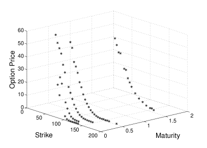
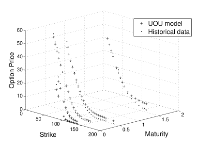
Figure 2: Market call price surface for IBM, July 7th, 2009 (left plot). Comparison of historical option prices and option prices calculated using the UOU model with the optimal parameter set (right plot).

To obtain the set of parameters for the primal probability measure, the UOU model is calibrated to the historical data from May 7th to July 7th, 2009. Using historical asset prices, $\widehat{S}_{t_{j}}$, $j=0,1,\ldots,N$, $0=t_{0}<t_{1}<\cdots<t_{N},$ and the transition densities, we obtain the following (single-asset) log-likelihood function for this set of observations:

$$L_{1}(\xi) =\sum_{j=1}^{N}\ln p_{S}(t_{j}-t_{j-1};\widehat{S}_{t_{j-1}},\widehat{S}_{t_{j}};\xi)$$ (3.4)

$$=\sum_{j=1}^{N}\ln\left(\frac{\nu}{\sigma(\widehat{S}_{t_{j}};\xi)}p_{X}^{(\rho)}\left(t_{j}-t_{j-1};\mathsf{X}(\widehat{S}_{t_{j-1}};\xi),\mathsf{X}(\widehat{S}_{t_{j}};\xi);\xi\right)\right).$$

Here, for simplicity, we assume the sequential simulation method. In case of a general sampling method, the log-likelihood function is given by

$$L_{1}(\xi)=\sum_{j=1}^{N}\ln\left(\frac{\nu}{\sigma(\widehat{S}_{\tilde{t}_{j}};\xi)}f_{j}\left(\mathsf{X}(\widehat{S}_{\tilde{t}_{j}};\xi);\xi\right)\right),$$ (3.5)

where $f_{j}$ is defined analogously to $f_{j}^{k}$ in Subsection 2.3 as if there was only one asset.

In practice, the implementation of the calibration procedure is started with some initial values of parameters. The upper and lower bounds for the parameters should also be provided. Based on the empirical analysis, such bounds are obtained and are provided in Table 1.

Table 1: Initial values and bounds for the parameters of the UOU model.

Parameter	$\rho$	$\upsilon$	$c$	$\kappa$
Lower bound	0.001	0.005	45	0.5
Upper bound	0.5	2	250	10
Initial value	0.04	0.34	102.59	1

The first step of the calibration procedure takes approximately $200$ seconds to fit the model to $63$ historical asset prices. The optimal values, that maximize the log-likelihood function (3.4), are $\rho=0.0357$, $\upsilon=0.0531$, $c=118.2404$, $\kappa=0.5951$. This set of parameters defines the primal probability measure $\mathds{P}_{0}$. The estimation of the regularization parameter $\alpha$ is based on the algorithm described above. The calculated value of $\alpha$ is $0.266$.

The final step of the calibration process is the minimization of the nonlinear least squares function regularized by the relative entropy as is given in (3.2). The computation algorithm utilizes the Matlab function lsqnonlin with the exit tolerance set to $10^{-6}$. This function employs the Levenberg-Marquardt least-squares algorithm for estimating optimal parameters. The starting values and the limits for the parameters remain the same as given in Table 1. The computational algorithm takes approximately 400 seconds to fit the model to 79 option prices. The best-fitted parameters of the model are $\rho=0.0203$, $\upsilon=0.0013$, $c=102.1384$, $\kappa=0.6579$. The objective function $F_{\alpha}$ attains its minimum value of 1.58.

Notice that the discrepancy between the computed option prices and observed option prices may originate from different sources. First, the market data may contain errors or misleading information. For example, the values of illiquid options might be mispriced, or simple input errors may occur. Second, the calibration procedure estimates model parameters of an arbitrage-free model, while the market prices are not necessarily arbitrage-free. Hence, there is an inherent mismatch between the model prices and the market data. Notice that the use of time-dependent parameters may decrease the level and number of errors and make the calibration procedure maturity-wise. Another possible solution to improve the accuracy is to employ the calibration separately for out-of-the-money, at-the-money and in-the-money options.

3.3 Multivariate Case

Let us consider the multi-asset price processes $(\mathbf{S}_{t})_{t\geq 0}$ modeled as described in Section 2, i.e. $n$ UOU diffusions are coupled via the Gaussian copula function.

The calibration procedure can be split into two stages: (1) estimation of the parameters of the marginal (single-asset price) processes; (2) estimation of the correlation matrix $R$ of the Gaussian copula. Such a calibration algorithm admits multiple variations. First, one may use the maximum likelihood estimation (MLE) to fit the marginal models to historical asset prices. Second, one may use the least-square method to fit the marginal models to historical derivative prices (say European options). For both approaches, the correlation matrix is then estimated by the MLE using historical asset prices. Alternatively, one may use only observed asset prices to estimate all parameter of the multivariate model simultaneously without splitting the calibration process. Notice also that the multivariate path distribution depends on the simulation method used. By using the sequential sampling or some version of the bridge sampling, one may obtain different models and, hence, obtain slightly different estimates of the model parameters.

Let $\left\{\mathbf{S}_{j}\equiv(\widehat{S}_{t_{j}}^{1},\ldots,\widehat{S}_{t_{j}}^{n})\right\}_{j=0}^{N}$ be the $n\times(N+1)$ matrix containing $N+1$ independent historical prices for each of the $n$ financial assets observed on a set of time points $T=\{t_{0},t_{1},\ldots,t_{N}\}$. Let $({\boldsymbol{\xi}},R)=(\xi_{1},\ldots,\xi_{n},R)$ denote the set of parameters to be estimated. The historical observations in $X^{(\rho)}$-space are obtained by applying the inverse map: $\widehat{X}^{k}_{t_{j}}=\mathsf{X}^{k}(\widehat{S}_{t_{j}}^{k};\xi_{k})$. Suppose the joint path PDFs of the $n$-dimensional processes $(\mathbf{X}_{t}^{(\boldsymbol{\rho})})$ and $(\mathbf{S}_{t})$ is constructed with the Gaussian copula as given by (2.6) and (2.7), respectively. The ($n$-asset) log-likelihood function is

$$\begin{split}L_{n}({\boldsymbol{\xi}},R)&=\ln\mathbb{f}^{s}(\mathbf{S}_{1},\ldots,\mathbf{S}_{N})=\sum_{j=1}^{N}\ln\mathbf{f}^{s}_{j}(\mathbf{S}_{j})\\ &=\sum_{j=1}^{N}\ln\phi_{R}(\mathcal{N}^{-1}(\Phi^{1}_{j}(\widehat{X}_{\tilde{t}_{j}}^{1};\xi_{1})),\ldots,\mathcal{N}^{-1}(\Phi^{n}_{j}(\widehat{X}_{\tilde{t}_{j}}^{n};\xi_{n})))\\ &\phantom{=}+\sum_{k=1}^{n}\sum_{j=1}^{N}\ln\left(\frac{\nu_{k}}{\sigma^{k}(\widehat{S}_{\tilde{t}_{j}}^{k})}f_{j}^{k}(\widehat{X}_{\tilde{t}_{j}}^{k};\xi_{k})\right)\equiv L_{n}^{\text{corr}}(R|{\boldsymbol{\xi}})+\sum_{k=1}^{n}L_{1}(\xi_{k}),\end{split}$$ (3.6)

where $\phi_{R}$ denotes the joint PDF of the $n$-variate normal distribution with mean vector zero, unit variances, and correlation matrix $R$; $L_{1}$ is the single-asset log-likelihood function given by (3.4) or (3.5), and $L_{n}^{\text{corr}}$ denotes the log-likelihood function for the copula function. Recall that the expression in (3.6) is independent of the simulation method used. For the sequential and bridge methods, we provide below specific expressions of the log-likelihood function.

As is suggested by the structure of the log-likelihood function in (3.6), the calibration process can be split into two steps. First, the sets $\xi_{k}=\left\{\lambda_{k},\nu_{k},c_{k},\rho_{k}\right\},\,k=1,2,\ldots,n$ of parameters of the marginal distributions are estimated by employing the maximum likelihood estimation:

$$\widehat{\xi}_{k}=\mathrm{arg}\max_{\xi_{k}}L_{1}(\xi_{k})=\mathrm{arg}\max_{\xi_{k}}\sum_{j=1}^{N}\ln\left(\frac{\nu_{k}}{\sigma^{k}(\widehat{S}_{\tilde{t}_{j}}^{k})}f_{j}^{k}(\widehat{X}_{\tilde{t}_{j}}^{k};\xi_{k})\right),\ \ k=1,\ldots,n.$$ (3.7)

As is seen, the parameters of the marginal distributions are estimated based on historical data. An alternative approach to computing the parameters is to fit asset price distributions to observed option prices as described in Subsection 3.1.

The last step is the estimation of the correlation matrix $R$ for the given optimal univariate model parameters $\mathbf{\widehat{\boldsymbol{\xi}}}\equiv\{\widehat{\xi}_{1},\ldots,\widehat{\xi}_{n}\}$, $\widehat{\xi}_{k}\equiv\left\{\hat{\lambda}_{k},\hat{\nu}_{k},\hat{c}_{k},\hat{\rho}_{k}\right\}$, estimated during the previous step.

First, we consider the sequential calibration method with the following log-likelihood function

$$L_{n}^{\text{corr}}(R|\widehat{\boldsymbol{\xi}})=\sum_{j=1}^{N}\ln\phi_{R}(\mathcal{N}^{-1}(\Phi^{1}_{j}(\widehat{X}_{{t}_{j}}^{1};\widehat{\xi}_{1})),\ldots,\mathcal{N}^{-1}(\Phi^{n}_{j}(\widehat{X}_{{t}_{j}}^{n};\widehat{\xi}_{n}))).$$ (3.8)

Sequential Calibration.

For the sequential path generation method, the algorithm is as follows.

1. Map all the observations into $X^{(\rho)}$-space using the respective inverse maps:

   $$\mathbf{X}_{j}\equiv(\widehat{X}_{j}^{1},\ldots,\widehat{X}_{j}^{n})=((\mathsf{X}^{1}(\widehat{S}_{t_{j}}^{1};\widehat{\xi}_{1}),\ldots,\mathsf{X}^{n}(\widehat{S}_{t_{j}}^{n};\widehat{\xi}_{n})),\ \ j=0,\ldots,N.$$

2. Compute vectors $\mathbf{u}_{j}\equiv(u_{j}^{1},\ldots,u_{j}^{n})\in[0,1]^{n},$ $j=1,\ldots,N,$ by evaluating the integrals:

   $$u^{k}_{j}=\int_{-\infty}^{\widehat{X}_{j}^{k}}p_{X}^{(\hat{\rho}_{k},k)}(t_{i}-t_{j-1};\widehat{X}_{j-1}^{k},x;\widehat{\xi}_{k})\,\mathrm{d}x,\ \ k=1,\ldots,n$$

3. Maximize the log-likelihood function with respect to $R$:

   $$L_{n}^{\text{corr}}(R|\widehat{\boldsymbol{\xi}})=\sum_{j=1}^{N}\ln\phi_{R}\left(\mathcal{N}^{-1}(u_{j}^{1}),\ldots,\mathcal{N}^{-1}(u_{j}^{n})\right)\to\max_{R}.$$

The estimation of the log-likelihood function for the sequential calibration involves numerous estimations of the CDF for the UOU model. Since there is no simple-form solution for the CDF, the numerical integration of the probability density function should be performed regularly. By applying the bridge approach to the construction of the multivariate path distribution function, the number of integrals to be computed numerically on step (ii) reduces from $n\times N$ to $n$. This is due to the fact that for the bridge approach, the CDF $\Phi^{k}_{j}$, $j=2,\ldots,N$, is Gaussian. Hence, for the bridge path generation method, the log-likelihood function can be simplified as follows:

$$\begin{split}L_{n}^{\text{corr}}(R|\widehat{\boldsymbol{\xi}})&=\sum_{j=2}^{N}\ln\phi_{R}\left(\dfrac{\widehat{X}_{\tilde{t}_{j}}^{1}-\mu_{kj}}{b_{kj}},\ldots,\dfrac{\widehat{X}_{\tilde{t}_{j}}^{n}-\mu_{kj}}{b_{kj}}\right)\\ &\phantom{=}+\ln\phi_{R}(\mathcal{N}^{-1}(\Phi_{1}^{1}(\widehat{X}_{\tilde{t}_{1}}^{1};\widehat{\xi}_{1})),\ldots,\mathcal{N}^{-1}(\Phi_{1}^{n}(\widehat{X}_{\tilde{t}_{1}}^{n};\widehat{\xi}_{n}))),\end{split}$$ (3.9)

where mean $\mu_{kj}$ and variance $b^{2}_{kj}$ computed by formulae in (1.14); and $\tilde{t}_{1}=T$.

Bridge Calibration.

The following algorithm can be applied for the backward-in-time bridge path generation method.

1. Map the observations into $X^{(\rho)}$-space $\mathbf{S}_{j}\rightarrow\mathbf{X}_{j}=\mathbf{F}^{-1}(\mathbf{S}_{j};\widehat{\boldsymbol{\xi}}),j=1,\ldots,N$, as is described in part (i) of the sequential algorithm.

2. Compute $\mathbf{u}_{N}\equiv(u_{N}^{1},\ldots,u_{N}^{n})$, the values of normal CDFs corresponding to the terminal point of a path:

   $$\begin{split}u_{N}^{k}=&\int_{-\infty}^{\widehat{X}^{k}_{N}}p_{X}^{(\hat{\rho}_{k},k)}(t_{N}-t_{N-1};\widehat{X}_{N-1}^{k},x;\widehat{\xi}_{k})\,\mathrm{d}x,\ \ k=1,\ldots,n.\\ \end{split}$$ (3.10)

3. For each $k=1,\ldots,n$ and $j=1,\ldots,N-1$ calculate $\mu_{kj}$ and $b_{kj}$ by using (1.14) with respective parameters $\lambda=\lambda_{k},$ $\kappa=\kappa_{k}$, $\Delta_{1}=t_{j}-t_{0},$ and $\Delta_{2}=t_{j+1}-t_{j}.$ Then, set

   $$x^{k}_{j}=\frac{\widehat{X}_{j}^{k}-\mu_{kj}}{b_{kj}}.$$

4. Maximize the log-likelihood function with respect to $R$:

   $$L_{n}^{\text{corr}}(R|\widehat{\boldsymbol{\xi}})=\sum_{j=1}^{N-1}\ln\phi_{R}\left(x^{1}_{j},\ldots,x^{n}_{j}\right)+\ln\phi_{R}\left(\mathcal{N}^{-1}(u_{N}^{1}),\ldots,\mathcal{N}^{-1}(u_{N}^{n})\right)\to\max_{R}.$$

Table 2: Optimal parameters estimated for IBM, Microsoft, Pepsi and Wallmart

	IBM	Microsoft	Pepsi	Wallmart
$\hat{\rho}$	0.0496	0.2173	0.0865	0.0493
$\hat{\upsilon}$	0.0887	0.0365	0.1149	0.0886
$\hat{c}$	103.9904	21.1638	31.671	52.3842
$\hat{\kappa}$	0.9670	0.874	0.910	0.9874

3.4 Numerical results for the multivariate case

For this numerical experiment the daily observations of four American companies, namely, IBM, Microsoft, Pepsi, and Wallmart, have been collected from Yahoo!${}^{\text{TM}}$. The examined period is April 7th, 2009, to July 7th, 2009, and it consists of 63 time points. In the first stage of the calibration, the optimal sets of parameters of the marginal distributions are estimated by solving Eq. (3.7), and they are provided in Table 2.

Two approaches are then used for the evaluation of the optimal correlation matrix $R$. In the first approach, the correlation matrix is obtained by the pairwise calculation of the correlation coefficients. There are $\binom{4}{2}$ correlation coefficients for $4$-asset price processes to be estimated. In other words, instead of solving a $4$-dimensional least-square problem with the log-likelihood function $L_{n}^{\text{corr}}$ given by (3.8) or (3.9), we independently solve $\binom{4}{2}$ $2$-dimensional problems with a 2-by-2 correlation matrix of the form $\left(\begin{array}[]{cc}1&\theta\\ \theta&1\end{array}\right)$ and then compose another 4-by-4 correlation matrix using the estimations of $\theta$.

However, the resulting matrix may violate the positive-definite property. To overcome this problem, a method suggested by [14] of finding the closest correlation matrix by the spectral decomposition is applied. The resulting matrices $\widehat{R}$ are shown in Table 3. The computation time is $32.6$ seconds for the bridge simulation and $47.9$ seconds for the sequential simulation.

Table 3: Correlation matrices obtained by using the bridge path simulation (left table) and the sequential path simulation (right table). The pairwise computation of the correlation coefficients is employed.

$$\small{\left(\begin{array}[]{rrrr}1&0.297&0.151&0.337\\ 0.297&1&0.089&-0.045\\ 0.151&0.089&1&-0.080\\ 0.337&-0.045&-0.080&1\\ \end{array}\right)};$$

$$\small{\left(\begin{array}[]{rrrr}1&0.278&0.243&0.336\\ 0.278&1&0.184&-0.050\\ 0.243&0.184&1&-0.051\\ 0.336&-0.050&-0.051&1\\ \end{array}\right)}.$$

In the second method, the correlation matrix as a whole is estimated. The computation of an optimal correlation matrix is performed in Matlab using the function fmincon, which allows us to find a minimum of a multivariate function with non-linear constraints. By adding nonlinear constraints, the algorithm works in the class of semi-positive matrices, which is absolutely necessary for the correct formulation of the correlation matrix. However, the candidate matrix, which minimizes the objective function in (3.6), may not have ones on the principal diagonal. To obtain a correct correlation matrix that is closest to the given one, the spectral decomposition method is applied again. The results are shown in Table 4 and Table 5.

Table 4: The candidate semi-positive matrix that minimizes the objective function $L_{n}^{\text{corr}}$ in (3.8) (left table) obtained by using the sequential simulation method and the closest correlation matrix obtained by using the spectral decomposition method (right table).

$$\small{\left(\begin{array}[]{rrrr}1.000&0.277&0.169&0.335\\ 0.277&0.993&0.127&-0.049\\ 0.169&0.127&0.480&-0.024\\ 0.335&-0.049&-0.024&0.993\\ \end{array}\right)}$$

$\underset{\text{decomp.}}{\overset{\text{spect.}}{\longrightarrow}}$ $$\small{\left(\begin{array}[]{rrrr}1&0.278&0.243&0.336\\ 0.278&1&0.183&-0.049\\ 0.243&0.183&1&-0.035\\ 0.336&-0.049&-0.035&1\\ \end{array}\right)}$$

Table 5: The candidate semi-positive matrix that minimizes the objective function $L_{n}^{\text{corr}}$ in (3.9) (left table) obtained by using the bridge simulation method and the closest correlation matrix obtained by using the spectral decomposition method (right table).

$$\small{\left(\begin{array}[]{rrrr}1.000&0.290&0.145&0.335\\ 0.290&0.973&0.084&-0.043\\ 0.145&0.084&0.966&-0.076\\ 0.335&-0.043&-0.076&0.993\\ \end{array}\right)}$$

$\underset{\text{decomp.}}{\overset{\text{spect.}}{\longrightarrow}}$ $$\small{\left(\begin{array}[]{rrrr}1&0.293&0.148&0.336\\ 0.293&1&0.086&-0.043\\ 0.148&0.086&1&-0.078\\ 0.336&-0.043&-0.078&1\\ \end{array}\right)}$$

4 Pricing Path-Dependent Options

4.1 Path-Dependent Multi-asset Options

Suppose the price process $(\mathbf{S}_{t})$ is modelled at a discrete set of time points (written in an increasing order) $\mathbf{T}=\{0=t_{0},t_{1},t_{2},\ldots,t_{N}=T\}$. Hence, we construct a multivariate discrete-time $n$-dimensional price path $(\mathbf{S}_{i})_{i=1,2,\ldots,N},$ where $\mathbf{S}_{j}=(S_{j}^{1},S_{j}^{2},\ldots,S_{j}^{n})$.

Let us consider two discrete-time monitored path-dependent securities, namely a Bermudan option and an Asian option. For an Asian-style option the payoff function $\Lambda_{N}(\mathbf{S}_{1},\ldots,\mathbf{S}_{N})$ is assumed to be a function of averages $A^{k}=\mathcal{A}\left(S_{1}^{k},\ldots,S_{N}^{k}\right)$ of the asset prices, where, for example in the case of the arithmetic time-averaging, ${A}^{k}=\frac{1}{N}\sum_{i=1}^{N}S_{i}^{k}$. The Asian basket option with the payoff

$$\Lambda_{N}=\left(\max\limits_{k=1}^{n}A^{k}-K\right)^{+},$$ (4.1)

considered in Section 4.2, is an example of an arithmetic average option.

The arbitrage-free value $V=V(\mathbf{S}_{0},\mathcal{T})$ of a discrete-time monitored path-dependent option (without early exercise opportunities) can be represented as a mathematical expectation under a risk-neutral probability measure $\mathds{Q}$:

$$V=e^{-rT}\mathds{E}^{\mathds{Q}}[\Lambda_{N}(\mathbf{S}_{1},\ldots,\mathbf{S}_{N})]=e^{-rT}\mathds{E}^{\mathds{Q}}[\Lambda_{N}(\mathbf{F}(\mathbf{X}_{1}),\ldots,\mathbf{F}(\mathbf{X}_{N}))]\,.$$ (4.2)

To find the option value one may use the Monte Carlo method.

The fair value of a Bermudan option cannot be represented in the form (4.2), but is a solution of some dynamic programming problem (see (4.3) below). Let $\Lambda(t,\mathbf{S})$ denote the payoff function for exercise at time $t$ in state $\mathbf{S}=\left(S^{1},\ldots,S^{n}\right)$. One may consider the two following examples of the time-homogeneous payoff function $\Lambda$:

• a max call option with the payoff $\Lambda(\mathbf{S})=\left(\max(S^{1},\ldots,S^{n})-K\right)^{+}$;

• a geometric average call with the payoff $\Lambda(\mathbf{S})=\left(\big{(}\prod\limits_{k=1}^{n}S^{k}\big{)}^{\frac{1}{n}}-K\right)^{+}$.

Let $V(t,\mathbf{S})$ denote the value of the option at time $t$ given $\mathbf{S}_{t}=\mathbf{S}$, assuming the option has not previously been exercised. We are interested in the present value $V(t_{0},\mathbf{S}_{0})$. This value is determined through the backward-in-time recursion:

$$\begin{array}[]{rcl}V(t_{N},\mathbf{S})&=&\Lambda(t_{N},\mathbf{S})\\ V(t_{i},\mathbf{S})&=&\max\left\{\Lambda(t_{i},\mathbf{S}),\mathds{E}^{\mathds{Q}}\left[e^{-r(t_{i+1}-t_{i})}V(t_{i+1},\mathbf{S}_{i+1})\mid\mathbf{S}_{i}=\mathbf{S}\right]\right\}\,,\end{array}$$ (4.3)

where $i=N-1,\ldots,0$. The risk-neutral expectation value function in the latter expression is called the continuation value function in state $\mathbf{S}$ at time $t_{i-1}$.

In our computational tests, the univariate models correspond to the model parameter values used to plot the local volatility function with the thick line in Figure 1. So, for the $\mathsf{UOU}$-family we simply set $\rho_{k}\equiv 0.02$, $\kappa_{k}=1$, $\upsilon_{k}=0.5$ and $c_{k}=100$, for all $k$. The interest rate is $r=0.05$.

4.2 Pricing Asian Basket Options

In this example we use the Monte Carlo method for pricing the arithmetic Asian basket call option with payoff function (4.1) under the multivariate UOU model. The Monte Carlo simulations were run on the SHARCNET network (http://www.sharcnet.ca). Mostly we use Gulper—a 42-CPU cluster. The code was written in FORTRAN-90 using the MPI library.

First, we present numerical results for a bivariate ($n=2$) UOU model. The correlation matrix used in the normal (Gaussian) copula has the usual form of $R=\left(\begin{array}[]{cc}1&\theta\\ \theta&1\end{array}\right)$. Table 6 provides the results of our numerical tests for the two-asset model. We used the following values of parameters: number of observations $N=100$, terminal time $T=1.0$, number of scenarios $M=10\,000\,000$, and spot value $S_{0}=100$.

Table 6: Pricing the Asian basket call option under the bivariate UOU model for different values of the correlation coefficient $\theta$ using the Monte Carlo method. A sample standard error is given after $\pm$ sign.

$K$	$\theta=-0.75$		$\theta=0$		$\theta=0.75$
90	31.538 $\pm$	0.008	27.942 $\pm$	0.008	22.444 $\pm$	0.009
100	22.786 $\pm$	0.007	20.409 $\pm$	0.008	16.168 $\pm$	0.007
110	15.614 $\pm$	0.007	14.348 $\pm$	0.007	11.321 $\pm$	0.006

The next example confirms that the computational complexity of the bridge copula method scales linearly with the number of assets. For all tests we use the crude Monte Carlo method on a single CPU. Clearly, the computational cost can be significantly reduced by using variance reduction methods and low-discrepancy point sets along with the parallel computing (see [7]). Another method of speeding up the computer code is to tabulate all distribution, generating and mapping functions that depend on the parabolic cylinder functions and other special functions.

Table 7 provides the results of our numerical tests for increasing numbers of assets. We use the same values of parameters as those of the previous test but reduce the number of scenarios to $M=1\,000\,000$. A 10-by-10 correlation matrix $R$ given in Figure 3 is generated using the random Gram matrix method from [12]. For values of $n<10$ we let $R$ be the $n\times n$-submatrix in the upper-left corner of the matrix given in Figure 3. Clearly, such a submatrix is again a correlation matrix of lower dimensionality.

$${\small\left(\begin{array}[]{r@{\,\,}r@{\,\,}r@{\,\,}r@{\,\,}r@{\,\,}r@{\,\,}r@{\,\,}r@{\,\,}r@{\,\,}r}1.000&0.550&-0.123&0.148&-0.239&0.238&0.239&0.096&0.289&-0.325\\ 0.550&1.000&-0.223&0.188&-0.109&0.396&-0.132&-0.118&0.237&-0.390\\ -0.123&-0.223&1.000&0.198&0.135&0.242&0.013&-0.731&0.244&-0.134\\ 0.148&0.188&0.198&1.000&-0.519&0.314&-0.191&-0.332&0.469&0.194\\ -0.239&-0.109&0.135&-0.519&1.000&-0.279&0.292&-0.044&-0.077&-0.443\\ 0.238&0.396&0.242&0.314&-0.279&1.000&0.023&0.050&0.049&-0.062\\ 0.239&-0.132&0.013&-0.191&0.292&0.023&1.000&0.423&-0.306&-0.292\\ 0.096&-0.118&-0.731&-0.332&-0.044&0.050&0.423&1.000&-0.417&0.152\\ 0.289&0.237&0.244&0.469&-0.077&0.049&-0.306&-0.417&1.000&-0.534\\ -0.325&-0.390&-0.134&0.194&-0.443&-0.062&-0.292&0.152&-0.534&1.000\end{array}\right)}$$

Figure 3: The 10-by-10 randomly generated correlation matrix $R$.

The idea of [12] is to generate independent pseudo-random vectors $\mathbf{u}_{1},\ldots,\mathbf{u}_{n}$ distributed uniformly on the $n$-dimensional unit sphere and then to use the Gram matrix $R=U^{\top}U$, where $U\equiv(\mathbf{u}_{1}|\cdots|\mathbf{u}_{n})$ has $\mathbf{u}_{k}$ as $k$th column and $U^{\top}$ is the transpose of $U$. To create $\mathbf{u}_{k}$ in $\mathds{R}^{n}$ we use a vector of independent standard normals $\mathbf{z}_{k}\sim\mathcal{N}(0,I)$ normalized by the Euclidian norm: $\mathbf{u}_{k}=\mathbf{z}_{k}/\|\mathbf{z}_{k}\|.$

Table 7: Pricing the Asian basket call option under the $n$-variate UOU model using the Monte Carlo method. A sample standard error is given after $\pm$ sign.

$K$	$n=2$		$n=3$		$n=5$		$n=10$
90	24.292 $\pm$	0.026	34.420 $\pm$	0.027	45.504 $\pm$	0.028	59.785 $\pm$	0.028
100	17.627 $\pm$	0.024	25.974 $\pm$	0.026	36.195 $\pm$	0.027	50.274 $\pm$	0.028
110	12.403 $\pm$	0.021	18.786 $\pm$	0.024	27.507 $\pm$	0.026	40.800 $\pm$	0.028
Time	3 745 sec		5 340 sec		8 389 sec		15 307 sec

4.3 Pricing Bermudan Options

Regression-based methods are broadly applied to pricing multivariate American options (see [11] and references therein). The main idea consists in the use of regression to estimate continuation values from simulated paths. Each continuation value is approximated by a linear combination of some basis functions. The coefficients of such a representation are estimated by a regression method (typically least-squares).

Consider an expression for the continuation value of the form:

$$\mathds{E}^{\mathds{Q}}\left[e^{-r(t_{i+1}-t_{i})}V(t_{i+1},\mathbf{S}_{i+1})\mid\mathbf{S}_{i}=\mathbf{S}\right]=\sum\limits_{q=1}^{L}\beta_{iq}\psi_{q}(\mathbf{S})=\beta_{i}^{\top}\psi(\mathbf{S}),$$ (4.4)

for some basis functions $\psi=(\psi_{1},\ldots,\psi_{L})^{\top}$, $\psi_{q}:\mathds{R}^{n}\to\mathds{R}$ and constants $\beta_{iq}$, $q=1,2,\ldots,L$, $i=0,1,\ldots,N-1$. An approximate value $\widehat{V}_{0}$ for the American (i.e. Bermudan) option price can be calculated by the following regression algorithm.

Regression-Based Pricing Algorithm.

1. Simulate $M$ independent asset price paths $(\mathbf{S}_{1j},\ldots,\mathbf{S}_{Nj}),$ $j=1,\ldots,M.$

2. At terminal nodes, set $\widehat{V}_{Nj}=\Lambda(t_{N},\mathbf{S}_{Nj}),$ $j=1,\ldots,M$.

3. Apply backward-in-time induction for $i=N-1,\ldots,1$:

   • Given estimated values $\widehat{V}_{i+1,j},$ $j=1,\ldots,M,$ the least-squared estimate of $\beta_{i}=(\beta_{i1},\ldots,\beta_{iR})^{\top}$ is given by $\widehat{\beta}_{i}=\widehat{B}^{-1}_{\psi,i}\widehat{B}_{\psi V,i}\,,$ where $\widehat{B}_{\psi,i}$ is the $L\times L$ matrix with $(r,q)$-entry $\frac{1}{M}\sum\limits_{j=1}^{M}\psi_{r}(\mathbf{S}_{ij})\psi_{q}(\mathbf{S}_{ij})$ and $\widehat{B}_{\psi V,i}$ is the $L$-vector with $q$th entry $\frac{e^{-r(t_{i+1}-t_{i})}}{M}\sum\limits_{j=1}^{M}\psi_{q}(\mathbf{S}_{ij})\widehat{V}_{i+1,j}.$

   • Set $\widehat{V}_{ij}=\max\left(\Lambda(t_{i},\mathbf{S}_{ij}),\sum\limits_{q=1}^{L}\widehat{\beta}_{iq}\psi_{q}(\mathbf{S}_{ij})\right)\,,j=1,\ldots,M$.

4. Set $\widehat{V}_{0}=(\widehat{V}_{11}+\ldots+\widehat{V}_{1M})/M$.

To illustrate the regression algorithm above, we consider a Bermudan put option on the maximum of two underlying assets $S_{1}$ and $S_{2}$ modeled by the UOU bridge copula with interest rate $r=0.05$, zero dividend yield, strike price $K=100$, time to maturity $T=1.0$, initial spot $S_{0}=100$, and $N=10$ exercise times distributed evenly in the time interval $[0,T]$. Here we use the same choice of the model parameters as in the previous numerical example. Clearly, this example can easily be extended to the case with three or more assets.

Table 8: Comparison of price estimates for Bermudan and European put options on the maximum of two assets modeled by the bridge copula multivariate UOU model with different values of the correlation coefficient $\theta$. A sample standard error is given after $\pm$ sign.

$\theta$	Bermudan		European
$-0.75$	3.336 $\pm$	0.002	1.831 $\pm$	0.002
$0$	7.106 $\pm$	0.003	5.680 $\pm$	0.003
$0.75$	11.580 $\pm$	0.004	10.798 $\pm$	0.005

In the regression algorithm the basis functions are the power functions $1,$ $S_{1},$ $S_{2},$ $S_{1}^{2},$ $S_{2}^{2},$ $S_{1}S_{2},$ and payoff function $\Lambda(S_{1},S_{2})=\left(K-\max(S_{1},S_{2})\right)^{+}.$ We apply the regression method with $M=100\,000$ independent paths. To calculate standard error we replicate the random estimator $100$ times. Table 8 shows numerical results for differing values of the correlation coefficient $\theta$. For comparison’s sake we also calculate the values of the European put option on the maximum of underlyings by the Monte Carlo method with $10^{7}$ sample paths.

Conclusion

In this paper we have constructed a new multi-asset pricing model, whose marginal (single-asset price) processes are nonlinear (local volatility smile) regular diffusions from a recently developed UOU family of probability conserving martingale models [5, 8]. The multivariate model is based on a bridge copula method, where a normal distribution function couples the underlying univariate Ornstein-Uhlenbeck bridges and consequently forms a multivariate asset price process with built-in correlations. Such an approach preserves the solvability of the model, hence the multivariate path density is available in closed form and can be used for the calibration of the model to market prices. Extra flexibility of the multivariate model is provided by different variations of the bridge sampling method. We are also able to sample multivariate paths from their exact distribution. Moreover, the proposed exact bridge simulation algorithm runs faster than any approximation scheme (e.g., the Euler method).

To illustrate the financial applications of our model, we succeeded in calibrating the model to single-asset equity option market prices as well as in calibrating the multi-asset price correlation matrix to historical asset prices. We also succeeded in pricing multi-asset Asian and Bermudan options by using a path integral Monte Carlo (MC) approach and an MC regression method, respectively. The preliminary calculations presented in this paper pave the way to further applications of derivatives pricing under such multi-asset state dependent diffusion models. The numerical efficiency of the path integral MC approach used in this paper can be further improved by employing quasi-MC methods. These methods have already been successfully used for another nonlinear model, the so-called Bessel-K model [5, 8], and are also applicable to the UOU local volatility smile model.

References

- [1] M. Abramowitz and I.A. Stegun. Handbook of Mathematical Functions, Dover, New York (1972).
- [2] C. Albanese, G. Campolieti, P. Carr, and A. Lipton, Black-Scholes goes hypergeometric, Risk 14 (2001) 99–103.
- [3] C. Albanese and G. Campolieti, Advanced Derivatives Pricing and Risk Management: Theory, Tools, and Hands-on Programming Applications, Elsevier Academic Press (2005).
- [4] A.N. Borodin and P. Salminen, Handbook of Brownian Motion – Facts and Formulae. Series: Probability and its Applications, Birkhäuser Basel, 2 edition (2002).
- [5] G. Campolieti and R. Makarov, On Properties of Some Analytically Solvable Families of Local Volatility Diffusion Models, submitted to Mathematical Finance (2006).
- [6] G. Campolieti and R. Makarov, Pricing path-dependent options on state dependent volatility models with a Bessel bridge, International Journal of Theoretical and Applied Finance 10 (2007) 1–38.
- [7] G. Campolieti and R. Makarov, Path Integral Pricing of Asian Options on State Dependent Volatility Models, Quantitative Finance 8:2 (2008) 147–161.
- [8] G. Campolieti and R. Makarov, Solvable Nonlinear Volatility Diffusion Models with Affine Drift, submitted to Stochastics: An International Journal of Probability and Stochastic Processes (2009).
- [9] R. Cont and P. Tankov, Financial modelling with jump processes, Chapman & Hall/CRC, Boca Raton (2004).
- [10] H.W. Engl, M. Hanke, A. Neubauer, Regularization of Inverse Problems, Kluwer Academic Publishers, Dordrecht (1996).
- [11] P. Glasserman, Monte Carlo methods in financial engineering, Springer-Verlag, New York (2004).
- [12] R.B. Holmes, On random correlation matrices. SIAM J. Matrix Anal. Appl., 12:2 (1991) 239–272.
- [13] W. Hörmann and J. Leydold, Continuous random variate generation by fast numerical inversion, ACM Trans. Model. Comput. Simul. 13 (2003) 347–362.
- [14] P. Jaeckel and R. Rebonato, The most general methodology for creating a valid correlation matrix for risk management and option pricing purposes, Journal of Risk 2:2 (Winter 1999/2000).
- [15] A. Kuznetsov, Solvable Markov processes, Ph.D. thesis, University of Toronto (2004).
- [16] R. Nelsen, An Introduction to Copulas, Springer, New York (1999).