Proceedings of SEAMS-GMU Conference 2007

Applied Mathematics, pp. 357–368.

Key words and Phrases: displaced phase-amplitude variables, nonlinear Schrödinger equation, breather solutions, amplitude amplification factor, wavefront dislocation.

1. INTRODUCTION

The nonlinear Schrödinger (NLS) equation is a nonlinear dispersive partial differential equation that has been used as a mathematical model in many areas of Mathematical Physics, such as nonlinear water waves, nonlinear optics and plasma physics (Ablowitz and Segur, 1981; Ablowitz and Clarkson, 1991). In this letter, we will consider the spatial NLS equation, given as follows:

$$\partial_{\xi}\psi+i\beta\partial_{\tau}^{2}\psi+i\gamma|\psi|^{2}\psi=0.$$ (1)

We will derive and study three exact solutions of this equation. These exact solutions are known in the literature as ‘breather’ solutions of the NLS equation (Dysthe and Trulsen, 1999; Dysthe, 2001; Grimshaw et. al., 2001). The name ‘breather’ reflects the behavior of the profile which is periodic in time or space and localized in space or time. The concept was introduced by Ablowitz, Kaup, Newell and Segur (Ablowitz, et. al., 1974) in the context of the sine-Gordon partial differential equation. The breather solutions are also found in other equations, for instance in the Davey-Stewartson equation (Tajiri and Arai, 2000) and modified Korteweg-de Vries (mKdV) equation (Drazin and Johnson, 1989).

To find the breather solutions of the NLS equation, we use a special Ansatz in the description with displaced phase-amplitude variables introduced by van Groesen et. al. (2006), with a displacement that depends on the background. Requiring the displaced phase to be temporally independent, has as consequence that the dynamics at each position is described by the motion of a nonlinear autonomous oscillator in a potential energy that depends on the phase and on the spatial phase change. It is remarkable that this assumption leads to the breather solutions of the NLS equation that are known in the literatures: the Soliton on Finite Background (SFB) (Akhmediev et. al., 1987), the Ma breather (Ma, 1979) and the rational breather (Peregrine, 1983). These solutions have been suggested as models for a class of freak wave events seen in $2+1$ dimensional simulations of surface gravity waves (Henderson et. al., 1999). However, the SFB shows many properties of extreme, or freak, rogue wave events, as observed by Osborne et. al. (2000), Calini and Schober (2002). The SFB is also a good candidate in order to generate extreme wave events in a hydrodynamic laboratory (Andonowati et. al., 2006; Huijsmans et. al., 2005).

This letter is organized as follows. Section 2 presents some exact solutions of the NLS equation. We demonstrate that three different solutions of the NLS equation are obtained within a similar formulation. Section 3 explains briefly the relationship among the solutions of the NLS equation. Section 4 will discuss the evolution of breather solutions in the Argand diagram. In Section 5 we will deal with surface water waves and observe the occurrence of wavefront dislocations in the corresponding density plots of the breather solutions. The final section draws some conclusions and remarks on the subject in this letter.

2. EXACT SOLUTIONS OF THE NLS EQUATION

The simplest nontrivial solution of the NLS equation is the plane-wave or the ‘continuous wave’ (cw) solution. It does not depend on the temporal variable $\tau$ and is given by $A_{0}(\xi)=r_{0}e^{-i\gamma r_{0}^{2}\xi}$. Another simple solution is the ‘one-soliton’ or ‘single-soliton’ solution. It can be found by the inverse scattering technique (Zakharov and Shabat, 1972), but also much simpler by seeking a travelling-wave solution. An explicit expression is given by

$$A(\xi,\tau)=A_{0}(\xi)\sqrt{2}\mathop{\rm sech}\nolimits\left(r_{0}\sqrt{\frac{\gamma}{\beta}}\tau\right).$$ (2)

It will become clear when we consider the corresponding physical wave field that both the cw and the one-soliton solutions have coherent structures, while other solutions that we will deal with below do not.

In van Groesen et. al. (2006), a displaced phase-amplitude description has been introduced. As a special case, we will look for a solution of the NLS equation in the form

$$A(\xi,\tau)=A_{0}(\xi)[G(\xi,\tau)e^{i\phi(\xi)}-1],$$ (3)

for which the phase $\phi$, which is ‘displaced’ since the background contribution is taken out, is taken to depend only on the spatial variable $\xi$. Substituting (3) into the NLS equation (1), we obtain two equations that correspond to the real and the imaginary parts, respectively.

Multiplying the real part by $\cos\phi$ and the imaginary part by $\sin\phi$, adding both equations will give a Riccati-like equation for $G$:

$$\partial_{\xi}G+\gamma r_{0}^{2}\sin 2\phi G-\gamma r_{0}^{2}\sin\phi G^{2}=0.$$ (4)

Solving this equation leads us to a conclusion that $G$ can be written in a special form. By letting $G=1/H$, then equation (4) becomes a first order linear differential equation in $H$:

$$\partial_{\xi}H-\gamma r_{0}^{2}\sin 2\phi\,H+\gamma r_{0}^{2}\sin\phi=0.$$ (5)

Let us take $\tilde{P}(\xi)=\textmd{exp}\left(-\gamma r_{0}^{2}\int\sin 2\phi(\xi)\,d\xi\right)$ as the integrating factor, multiply it to (5) and integrate the result with respect to $\xi$, then we obtain the solution for $H$:

$$H(\xi,\tau)=\frac{-\gamma r_{0}^{2}\int\tilde{P}(\xi)\sin\phi(\xi)\,d\xi-\zeta(\tau)}{\tilde{P}(\xi)}=\frac{\tilde{Q}(\xi)-\zeta(\tau)}{\tilde{P}(\xi)},$$ (6)

where $-\zeta(\tau)$ is a constant of integration that depends on $\tau$ and $\tilde{Q}(\xi)$ denotes the term with the integral sign. Assuming that the displaced phase $\phi(\xi)$ is an invertible function, we can write $\xi=\xi(\phi)$ and dropping the tilde signs to indicate that $P=P(\phi)$ and $Q=Q(\phi)$. Consequently, $G$ is now written as follows:

$$G(\phi,\tau)=\frac{P(\phi)}{Q(\phi)-\zeta(\tau)}.$$ (7)

We will observe in the following subsections that by choosing three different functions of $\zeta(\tau)$ will lead to three different breather solutions of the NLS equation.

On the other hand, multiplying the real part by $\sin\phi$ and the imaginary part by $\cos\phi$, subtracting one from the other we obtain a nonlinear oscillator equation for $G$:

$$\beta\partial_{\tau}^{2}G+(\phi^{\prime}(\xi)+2\gamma r_{0}^{2}\cos^{2}\phi)G-3\gamma r_{0}^{2}\cos\phi G^{2}+\gamma r_{0}^{2}G^{3}=0.$$ (8)

In deriving the breather solutions, we will compare this equation with the second order differential equation for $G$ after choosing a particular function of $\zeta(\tau)$.

2.1 Soliton on Finite Background

Firstly, we take $\zeta(\tau)=\cos(\nu\tau)$, where $\nu$ is a modulation frequency. For the normalized quantity $\tilde{\nu}=\nu/\left(r_{0}\sqrt{\frac{\gamma}{\beta}}\right)$ we consider $0<\tilde{\nu}<\sqrt{2}$. The differential equation for $G$ becomes:

$$\partial_{\tau}^{2}G=-\nu^{2}G+3\nu^{2}\frac{Q}{P}G^{2}+2\nu^{2}\frac{1-Q^{2}}{P^{2}}G^{3}.$$

By comparing with (8), the solution (7) is obtained with $P(\phi)=\tilde{\nu}^{2}Q(\phi)/\cos\phi$, $Q^{2}(\phi)=2\cos^{2}\phi/(2\cos^{2}\phi-\tilde{\nu}^{2})$ and the displaced phase satisfies $\tan\phi(\xi)=-\frac{\tilde{\sigma}}{\tilde{\nu}^{2}}\tanh(\sigma\xi)$, where $\tilde{\sigma}=\tilde{\nu}\sqrt{2-\tilde{\nu}^{2}}$ and $\sigma=\gamma r_{0}^{2}\tilde{\sigma}$. The corresponding solution of the NLS equation (3) with extremum at $(\xi,\tau)=(0,0)$ can then be written after some manipulations as:

$$A(\xi,\tau)=A_{0}(\xi)\cdot\left(\frac{\tilde{\nu}^{2}\cosh(\sigma\xi)-i\tilde{\sigma}\sinh(\sigma\xi)}{\cosh(\sigma\xi)-\sqrt{1-\frac{1}{2}\tilde{\nu}^{2}}\cos(\nu\tau)}-1\right).$$

This solution was found by Akhmediev et. al. (1987). They suggested a method of obtaining exact solutions of the NLS equation which is based on the substitution connecting the real and imaginary parts of the solution by a linear relationship with coefficients depending only on time. The method consists in constructing a certain system of ordinary differential equations, the solutions of which determine the solutions of the NLS equation. However, the explicit expression of the SFB already appeared in the previous papers (Akhmediev et. al. 1985; Akhmediev and Korneev, 1986). The SFB is also derived by Ablowitz and Herbst (1990) using Hirota’s method (Hirota, 1976) and for $\tilde{\nu}=1$ by Osborne et. al. (2000) using the inverse scattering technique. The SFB is the single homoclinic orbit to the cw as a fixed point of the NLS equation (Ablowitz and Herbst, 1990; Li and McLaughlin, 1994, 1997; Calini and Schober, 2002). The asymptotic behaviour for $\xi\rightarrow-\infty$ of the SFB describes the linear instability of the cw solution for side-band perturbation (Akhmediev and Korneev, 1986). This modulational instability is known as the Benjamin-Feir instability in the context of water waves (Benjamin and Feir, 1967). A plot of the absolute value of this complex amplitude solution for $r_{0}=1$ and $\tilde{\nu}=1/2$ is given in Figure 1(a).

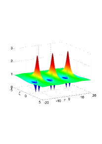
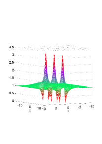
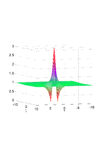
Figure 1: Plots of the absolute value of the SFB breather for $\tilde{\nu}=1/2$ (left), the Ma breather for $\tilde{\mu}=0.4713$ (center) and the rational breather (right), for $r_{0}=1$ in all cases. For illustration purposes, the axis are scaled corresponding to $\beta=1=\gamma$.

2.2 Ma breather

Secondly, we take $\zeta(\tau)=\cosh(\mu\tau)$, where $\mu=r_{0}\sqrt{\frac{\gamma}{\beta}}\tilde{\mu}$. The differential equation for $G$ becomes:

$$\partial_{\tau}^{2}G=\mu^{2}G-3\mu^{2}\frac{Q}{P}G^{2}-2\mu^{2}\frac{1-Q^{2}}{P^{2}}G^{3}.$$

Comparing again with (8), the solution (7) is obtained with $P(\phi)=-\tilde{\mu}^{2}Q(\phi)/\cos\phi$, $Q^{2}(\phi)=2\cos^{2}\phi/(2\cos^{2}\phi+\tilde{\mu}^{2})$ and the displaced phase satisfies $\tan\phi(\xi)=-\frac{\tilde{\rho}}{\tilde{\mu}^{2}}\tan(\rho\xi)$, where $\tilde{\rho}=\tilde{\mu}\sqrt{2+\tilde{\mu}^{2}}$ and $\rho=\gamma r_{0}^{2}\tilde{\rho}$. The corresponding solution of the NLS (3) can then be written after some manipulations as:

$$A(\xi,\tau)=A_{0}(\xi)\cdot\left(\frac{-\tilde{\mu}^{2}\cos(\rho\xi)+i\tilde{\rho}\sin(\rho\xi)}{\cos(\rho\xi)-\sqrt{1+\frac{1}{2}\tilde{\mu}^{2}}\cosh(\mu\tau)}-1\right).$$

We call this solution Ma solution or Ma breather since it has been found by Ma (1979) using the inverse scattering technique of (Gardner et. al., 1967). The same technique is also used by Osborne et. al. (2000) to arrive at this solution for $\tilde{\mu}=\sqrt{2}$. A plot of the absolute value of the Ma breather for $r_{0}=1$ and $\tilde{\mu}=0.4713$ is given in Figure 1(b). This choice of this value of $\tilde{\mu}$ is just for our convenience, which we will use again for the corresponding physical wave field.

2.3 Rational breather

Thirdly, we take $\zeta(\tau)=1-\frac{1}{2}\nu^{2}\tau^{2}$. Similarly, the same solution can also be obtained by substituting $\zeta(\tau)=1+\frac{1}{2}\mu^{2}\tau^{2}$. As a consequence, the differential equation for $G$ now becomes:

$$\partial_{\tau}^{2}G=\frac{3\nu^{2}}{P}G^{2}-4\nu^{2}\frac{Q-1}{P^{2}}G^{3}.$$

Comparing again with (8), we have $P(\phi)=\tilde{\nu}^{2}/\cos\phi$, $Q(\phi)=1+P^{2}/(4\tilde{\nu}^{2})$ and the displaced phase satisfies $\tan\phi(\xi)=-2\gamma r_{0}^{2}\xi$. Substituting into the Ansatz (7), we obtain

$$A(\xi,\tau)=A_{0}(\xi)\cdot\left(\frac{4(1-2i\gamma r_{0}^{2}\xi)}{1+4(\gamma r_{0}^{2}\xi)^{2}+2\frac{\gamma}{\beta}r_{0}^{2}\tau^{2}}-1\right).$$

This rational solution is clearly different from the two solutions above, is derived by Peregrine (1983) as a limiting case from the Ma breather. He took the analytic expression and performed a double Taylor series expansion about the amplitude peak (which occur at $\xi=0=\tau$) to arrive at his solution. Since this solution is confined in both space and time, some authors (Henderson et. al., 1999) also called it the ‘isolated Ma soliton’ and other authors (Akhmediev and Ankiewicz, 1997) called it the ‘rational solution’. Because of its soliton-like feature in $\xi$, (Nakamura and Hirota, 1985) called it as an ‘explode-decay solitary wave’. In this letter, we call it the ‘rational breather’. A plot of the absolute value of the rational breather for $r_{0}=1$ is given in Figure 1(c).

3. RELATION BETWEEN THE NLS BREATHER SOLUTIONS

As shown by Dysthe and Trulsen (1999), there is a relationship among the breather solutions of the NLS equation. Different parameters are used for explicit expressions of the SFB and the Ma breather in Dysthe and Trulsen (1999) as well as in Grimshaw et. al. (2001). Introducing new parameters $\varphi$ and $\vartheta\in\mathbb{R}$ by the following relations: $\tilde{\nu}=\sqrt{2}\sin\varphi$, $\tilde{\sigma}=\sin 2\varphi$, $\tilde{\mu}=\sqrt{2}\sinh\vartheta$ and $\tilde{\rho}=\sinh 2\vartheta$, we can write our expressions similar to the ones in these papers.

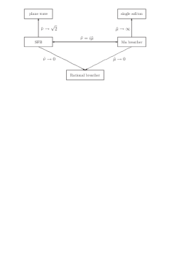
Figure 2: The schematic diagram for the derivation of the Ma breather and the rational breather from the SFB.

The SFB becomes the Ma breather if we substitute $\nu=i\mu$ and it becomes the rational breather if $\nu\rightarrow 0$. Similarly, the Ma breather becomes the rational breather for $\mu\rightarrow 0$. Interestingly, the Ma breather becomes the one-soliton solution for $\mu\rightarrow\infty$ (Akhmediev and Ankiewicz, 1997). Figure 2 explains the schematic diagram of these derivations. These relations can also be seen from the expression in the previous section. For the SFB, we take $\zeta(\tau)=\cos(\nu\tau)$, which leads to the Ma breather if we substitute $\nu=i\mu$, so that $\zeta(\tau)=\cos(i\mu\tau)=\cosh(\mu\tau)$. Taking either $\nu$ or $\mu$ $\rightarrow 0$, we get $\zeta(\tau)=1-\frac{1}{2}\nu^{2}\tau^{2}$ or $\zeta(\tau)=1+\frac{1}{2}\mu^{2}\tau^{2}$, and both will lead to the rational breather.

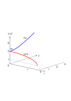
Figure 3: Plot of the amplitude amplification factor for the SFB and the Ma breather. The meeting point of the two curves is the AAF of the rational breather.

The relations have also consequence for the amplitude amplification factor (AAF), defined as the ratio between the maximum amplitude and the value of its background. The expressions for the breather solutions as given in this letter were shifted such that the maximum amplitude is at $(\xi,\tau)=(0,0)$ and the value of the background is $r_{0}$. For the SFB, the amplification is given by $\textmd{AAF}_{\textmd{\tiny S}}(\tilde{\nu})=1+\sqrt{4-2\tilde{\nu}^{2}}$. For $0<\tilde{\nu}<\sqrt{2}$, the amplification is bounded and are $1<\textmd{AAF}_{\textmd{\tiny S}}(\tilde{\nu})<3$. The AAF for the Ma breather is given by $\textmd{AAF}_{\textmd{\tiny Ma}}(\tilde{\mu})=1+\sqrt{4+2\tilde{\mu}^{2}}$. Hence, for $\tilde{\mu}>0$, we have $\textmd{AAF}_{\textmd{\tiny Ma}}>3$. The AAF for the rational breather is exactly $3$, which follows by letting the either $\tilde{\nu}$ or $\tilde{\mu}$ go to zero

$$\textmd{AAF}_{\textmd{\tiny Ra}}=\lim_{\tilde{\nu}\rightarrow 0}\textmd{AAF}_{\textmd{\tiny S}}=3=\lim_{\tilde{\mu}\rightarrow 0}\textmd{AAF}_{\textmd{\tiny Ma}}.$$ (9)

In Onorato et. al. (2001), the AAF for the SFB is given as a function of the wave steepness and the number of waves under the modulation. The plot of the AAF for all the three breather solutions is given in Figure 3. For $\tilde{\mu}\rightarrow\infty$ in the Ma breather, the single-soliton solution is obtained (Akhmediev and Ankiewicz, 1997).

4. EVOLUTION IN THE ARGAND DIAGRAM

In this section we present the evolution of the breather solutions in a complex plane. The real and the imaginary axes of this plane are denoted by the real and the imaginary part of the breather solutions after removing the plane-wave contribution, respectively. In this paper we refer this plane as the Argand diagram. Since the breather solutions depend on the space variable $\xi$ and the time variable $\tau$, the evolution curves are presented by parameterizing one variable and plotting for the other at different values. We will observe that the point $(-1,0)$ plays a significant role with respect to all evolution curves, whether they are parameterized in space or in time. A study of this evolution curves for understanding experimental results on freak wave generation using the SFB solution has been presented recently (Karjanto, 2006).

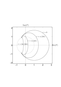
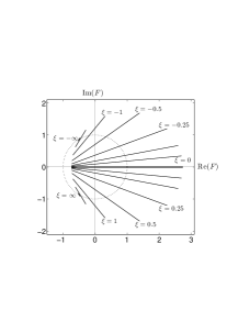
Figure 4: The evolution of the SFB in the Argand diagram for $\tilde{\nu}=1/\sqrt{2}$.

Figure 4 shows the evolution curves of the SFB for $\tilde{\nu}=1/\sqrt{2}$. The parameterized plot in position for different times is given by Figure 4(a). For this particular value of modulation frequency $\tilde{\nu}$, all curves start from a point in the second quadrant, which corresponds to $\xi=-\infty$, and end to a point in the third quadrant, which corresponds to $\xi=\infty$. During one modulation period $0\leq\tau<2\pi/\tilde{\nu}$, we observe that the curve reaches its maximum value for $\tau=0$ when the Im($F$) vanishes and it reaches a minimum value for $\tau=\pi/\tilde{\nu}$. The dotted circle indicates the plane wave solution that has been removed. When we allow the modulation frequency $\tilde{\nu}\rightarrow 0$, both the initial and the final points will coincide at $(-1,0)$, as shown by the rational breather case in Figure 6(a). The parameterized plot in time for different positions is given by Figure 4(b). All curves are straight lines and they are passed twice during one modulation period. For $\xi\rightarrow\pm\infty$, the lines shrink to a point in the third and the second quadrants, respectively. The longest line is reached at $\xi=0$ when it lies on the real axis. Notice that $(-1,0)$ becomes a center for all the lines. Moreover, for $\tilde{\nu}\rightarrow 0$, the left-hand side of all the lines will meet at $(-1,0)$, as shown by the rational breather case in Figure 6(b).

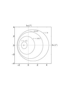
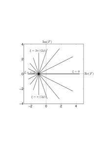
Figure 5: The evolution of the Ma breather in the Argand diagram for $\tilde{\mu}=2$.

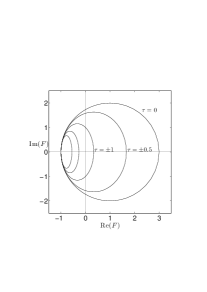
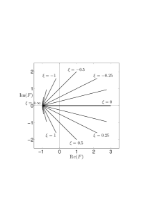
Figure 6: The evolution of the rational breather in the Argand diagram.

Figure 5 shows the evolution curves of the Ma breather for $\tilde{\mu}=2$. The parameterized plot in position for different times is given by Figure 5(a). All the curves are elliptical, which indicate that they are $\xi$-periodic. The largest curve occurs at $\tau=0$, which has a circular form. As the time moves forward and backward, the ellipses are getting smaller until eventually shrink to a point at $(-1,0)$ for $\tau=\pm\infty$. By letting $\tilde{\mu}\rightarrow 0$, the left-hand side of the ellipses at the real axis moves accordingly toward $(-1,0)$, and eventually the pattern becomes the one as shown by the rational breather in Figure 6(a). The parameterized plot in time for different positions is given by Figure 5(b). Similar to the previous case, all the curves are straight lines and we notice clearly that they are centered at $(-1,0)$. Different from the SFB solution case where the lines are at the right-hand side of $(-1,0)$, for the Ma breather case the point radiates lines to all different direction depending on the position. For one periodic position $0\leq\xi<2\pi/\tilde{\rho}$, the longest line occurs at $\xi=0$ and the shortest one occurs at $\xi=\pi/\tilde{\rho}$, being both of them lay on the real axis. When $\tilde{\mu}\rightarrow 0$, the lines which are on the left-hand side of $(-1,0)$ will get shorter until eventually become the rational breather case as shown in Figure 6(b). Figure 6 shows the evolution curves of the rational breather, which show the limiting cases for both $\tilde{\nu}\rightarrow 0$ and $\tilde{\mu}\rightarrow 0$.

5. PHYSICAL WAVE FIELDS

In this section, we show applications in surface water waves. Since the NLS equation is an envelope equation, the corresponding physical wave fields $\eta(x,t)$ are wave packets. Considering only first order contributions, the physical wave field is given by

$$\eta(x,t)=A(\xi,\tau)e^{i(k_{0}x-\omega_{0}t)}+\textmd{c\,c}$$ (10)

where c c denotes complex conjugate of the preceding term. The complex amplitude $A$ is described in a moving frame of reference with $\xi=x$ and $\tau=t-x/V_{0}$. The wavenumber $k_{0}$ and the frequency $\omega_{0}$ are related by the linear dispersion relation. For surface water waves, the normalized form of the dispersion relation is given by $\omega=\Omega(k)=k\sqrt{(\tanh k)/k}$, the group velocity $V_{0}=\Omega^{\prime}(k_{0})$.

Density plots for three breather solutions are given in Figure 7. For illustrations, we choose $r_{0}=1$, $k_{0}=2\pi$ ($\omega_{0}\approx\sqrt{2\pi}$) in all cases, modulation frequency $\tilde{\nu}=1/2$ for the SFB and $\tilde{\mu}=0.4713$ for the Ma breather. For better representation, the physical wave fields are shown in a moving frame of reference with suitable chosen group velocity. The SFB has extreme values at $x=\xi=0$ and is periodic in time. The Ma breather has extreme values at $\tau=0$ and is periodic in space. The rational breather is neither periodic in time nor in space, but isolated with its maximum at $(x,t)=(0,0)$. Despite some differences, all the breather solutions show ‘wavefront dislocation’, when splitting or merging of waves occurs (Nye and Berry, 1974). A necessary condition for this phenomenon to occur is that the Chu-Mei quotient of the nonlinear dispersion relation at the vanishing amplitude is unbounded. When it occurs, the real-valued phase of the corresponding wave field is undefined at the vanishing amplitude, known as ‘phase singularity’. More information on wavefront dislocation in surface water waves can be found in (Tanaka, 1995; Karjanto and van Groesen, 2007).

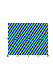
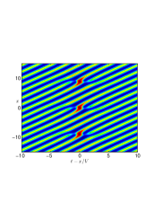
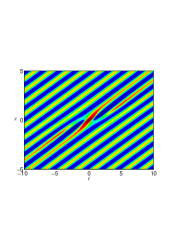
Figure 7: Density plot of the physical wave field of the SFB for $\tilde{\nu}=1/2$ (left), the Ma breather for $\tilde{\mu}=0.4713$ (center) and the rational breather (right) corresponding to Figure 1 for $k_{0}=2\pi$. The plots are shown in a moving frame of reference with suitable chosen velocity.

6. CONCLUSIONS

In this letter, we have shown that a description with displaced phase-amplitude variables, for which the phase is time independent, leads to the three breather solutions of the NLS equation: the Soliton on Finite Background, the Ma breather, and the rational breather. These are obtained as explicit solutions of the equation for the displaced amplitude of the NLS equation. We described the relation between these three breather solutions and presented the amplitude amplification factor of each solution as function of the parameters. For the corresponding physical wave fields, wavefront dislocation and phase singularity at vanishing amplitude are observed in all three cases.

Acknowledgement. Partly of this work is executed at University of Twente, The Netherlands as part of the project ‘Prediction and generation of deterministic extreme waves in hydrodynamic laboratories’ (TWI.5374) of the Netherlands Organization of Scientific Research NWO, subdivision Applied Sciences STW.

REFERENCES

• M. J. Ablowitz, et. al. The inverse scattering transform-Fourier analysis for nonlinear problems, Stud. Appl. Math., 53, 249-315, 1974.

• M. J. Ablowitz and H. Segur, Solitons and Inverse Scattering Transform, Society for Industrial and Applied Mathematics, Philadelphia, 1981.

• M. J. Ablowitz and B. M. Herbst, On homoclinic structure and numerically induced chaos for the NLS equation, SIAM J. Appl. Math., 50, 2:339-351, 1990.

• M. J. Ablowitz and P. A. Clarkson, Solitons, Nonlinear Evolution Equations and Inverse Scattering, volume 149 of London Mathematical Society Lecture Note Series. Cambridge University Press, 1991.

• N. N. Akhmediev, V. M. Eleonski$\breve{\textmd{i}}$ and N. E. Kulagin, Generation of periodic trains of picosecond pulses in an optical fiber: exact solutions, Sov. Phys. JETP, 62, 5: 894-899, 1985.

• N. N. Akhmediev and V. I. Korneev, Modulation instability and periodic solutions of the nonlinear Schrödinger equation, Teoret. Mat. Fiz., 62, 2:189-194, 1986. English translation: Theoret. Math. Phys. 69, 1089-1092, 1986.

• N. N. Akhmediev, V. M. Eleonski$\breve{\textmd{i}}$, and N. E. Kulagin, First-order exact solutions of the nonlinear Schrödinger equation, Teoret. Mat. Fiz., 72, 2:183-196, 1987. English translation: Theoret. Math. Phys., 72, 2:809-818, 1987.

• N. N. Akhmediev and A. Ankiewicz, Solitons—Nonlinear Pulses and Beams, volume 5 of Optical and Quantum Electronic Series, Chapman & Hall, first edition, 1997.

• Andonowati, N. Karjanto and E. van Groesen, Extreme wave phenomena in down-stream running modulated waves, Appl. Math. Model., 31, 1425–1443, 2007.

• T. B. Benjamin and J. E. Feir, The disintegration of wave trains on deep water. Part 1. Theory., J. Fluid Mech., 27, 3:417-430, 1967.

• A. Calini and C. M. Schober, Homoclinic chaos increases the likelihood of rogue wave formation, Phys. Lett. A, 298, 335-349, 2002.

• P. G. Drazin and R. S. Johnson, Solitons: an Introduction, Cambridge University Press, 1989.

• K. B. Dysthe and K. Trulsen, Note on breather type solutions of the NLS as models for freak-waves, Phys. Scripta, T82, 48-52, 1999.

• K. B. Dysthe, Modelling a “rogue wave”–speculations or a realistic possibility? In M. Olagnon and G. A. Athanassoulis, editors, Proceedings Rogue Waves 2000, Ifremeer, Brest, France, 2001.

• C. S. Gardner, J. M. Greene, M. D. Kruskal and R. M. Miura, Method for solving the Korteweg-de Vries equation, Phys. Rev. Lett. 19, 19:1095-1097, 1967.

• R. Grimshaw, D. Pelinovsky, E. Pelinovsky and T. Talipova, Wave group dynamics in weakly nonlinear long-wave models, Physica D 159, 35-37, 2001.

• K. L. Henderson, D. H. Peregrine, and J. W. Dold, Unsteady water wave modulations: fully nonlinear solutions and comparison with the nonlinear Schrödinger equation. Wave Motion, 29, 341-361, 1999.

• R. Hirota, Direct method of finding exact solutions of nonlinear evolution equations, in R. M. Miura, editor, Bäcklund Transformations, the Inverse Scattering Method, Solitons, and Their Applications, Springer-Verlag, Berlin, 1976.

• R. H. M. Huijsmans, G. Klopman, N. Karjanto and Andonowati, Experiments on extreme wave generation using the Soliton on Finite Background, in M. Olagnaon and M. Prevosto, editors, Proceedings Rogue Waves 2004, Ifremer, Brest, France, 2005.

• N. Karjanto, Mathematical Aspects of Extreme Water Waves, PhD thesis, University of Twente, 2006.

• N. Karjanto and E. van Groesen, Note on wavefront dislocation in surface water waves, Phys. Lett. A, 37, 173-179, 2007.

• Y. Li and D. W. McLaughlin, Morse and Melnikov functions for NLS PDE’s, Commun. Math. Phys., 162, 175-214, 1994.

• Y. Li and D. W. McLaughlin, Homoclinic orbits and chaos in discretized perturbed NLS systems: Part I. Homoclinic orbits, J. Nonlinear Sci., 7, 211-269, 1997.

• Y.-C. Ma, The perturbed plane-wave solutions of the cubic Schrödinger equation, Stud. Appl. Math., 60, 1:43-58, 1979.

• A. Nakamura and R. Hirota, A new example of explode-decay solitary waves in one dimension, J. Phys. Soc. Japan, 54, 2:491-499, 1985.

• J.F. Nye and M.V. Berry, Dislocation in wave trains, Proc. R. Soc. Lond. A, 336, 1065:165-190, 1974.

• M. Onorato, A. Osborne, M. Serio and T. Damiani, Occurrence of freak waves from envelope equations in random ocean wave simulations, in M. Olagnon and G. A. Athanassoulis, editors, Proceedings Rogue Waves 2000, Ifremer, Brest, France, 2001.

• A. R. Osborne, M. Onorato and M. Serio, The nonlinear dynamics of rogue waves and holes in deep-water gravity wave trains, Phys. Lett. A, 275, 386-393, 2000.

• D. H. Peregrine, Water waves, nonlinear Schrödinger equations and their solutions, J. Austral. Math. Soc. Ser. B, 25, 1:16-43, 1983.

• M. Tanaka, Dissapearance of waves in modulated train of surface gravity waves, Structure and Dynamics of Nonlinear Waves in Fluids, in A. Mielke and K. Kirchgässner, editors, IUTAM/ISIMM Symposium Proceedings (Hannover, August 1994), volume 7 of Advanced Series in Nonlinear Dynamics, World Scientific, Singapore, 392-398, 1995.

• M. Tajiri and T. Arai, Periodic soliton solutions to the Davey-Stewartson equation, Proc. Inst. Math. Natl. Acad. Sci. Ukr., 30, 1:210-217, 2000.

• E. van Groesen, Andonowati and N. Karjanto, Displaced phase-Amplitude variables for waves on finite background, Phys. Lett. A, 354, 312-319, 2006.

• V. E. Zakharov and A. B. Shabat, Exact theory of two-dimensional self-focusing and one-dimensional self-modulation of waves in nonlinear media, Sov. Phys. JETP, 34, 1:62-69, 1972.

Natanael Karjanto: School of Applied Mathematics, The University of Nottingham Malaysia Campus, Jalan Broga, 43500 Semenyih, Selangor Darul Ehsan, Malaysia.
E-mail: natanael.karjanto@nottingham.edu.my

E. van Groesen: Department of Applied Mathematics, University of Twente, P.O. Box 217, 7500 AE Enschede, The Netherlands.
E-mail: groesen@math.utwente.nl