A General Inverse Problem for the Growth-Fragmentation Equation
Abstract
Aggregation-fragmentation equations arise in many different contexts, ranging from cell division, protein polymerization, biopolymers, neurosciences etc. Direct observation of temporal dynamics being often difficult, it is of main interest to develop theoretical and numerical methods to recover reaction rates and parameters of the equation from indirect observation of the solution. Following the work done in [2] and [3] for the specific case of the cell division equation, we address here the general question of recovering the fragmentation rate of the equation from the observation of the time-asymptotic solution, when the fragmentation kernel and the growth rates are fully general. We give both theoretical results and numerical methods, and discuss the remaining issues.
keywords. Growth-Fragmentation equation ; general fragmentation kernels ; inverse problem ; eigenvalue problem.
MSC Classification. 35Q92, 35R30, 45Q05.
Introduction
To model the behavior of a population where growth and division depend on a structuring quantity of the individuals such as size, the following mass-balance equation is currently used:
| (1) |
Here, denotes the density of the individuals structured by the size variable at time the growth rate is given by ; the division rate represents the rate at which a given individual of size gives birth to two individuals of size respectively and whereas is the total rate of division for individuals of size This physical interpretation of leads to the following assumptions:
| (2) |
By simple integration and symmetry, it leads to the following well-known relation, expressing the conservation of mass by the division process:
Problem (1) or its variants arises in many different contexts, ranging from cell division, protein polymerization, telecommunication, neurosciences, and its mathematical study can provide useful information on the qualitative behavior of the phenomenon under consideration (see, among many others, [12, 13]). To be able to use it as a predictive model however, it is crucial to be able to estimate quantitatively its parameters and
A first step consists in the use of the asymptotic behavior of this equation, as first proposed in [2]. Indeed, by general relative entropy principle it is proven (see e.g [14, 15, 5]) that under suitable assumptions on , and one has
with and is the unique eigenpair solution of the following problem:
| (3) |
The use of this new problem allows to restrict the need for information to a non-temporal measure, and the problem becomes: How to recover information on and from an experimental measurement of the asymptotic profile and the global exponential rate of growth of the population 111Growth can naturally be balanced by death, by the addition for instance of a death term on the left-hand side of the equation. This would lead to possible nonpositive rates but our whole study would remain unchanged. ?
In the case when the equation models cell-division, direct measures of the growth rate is possible. Direct measures of is also possible, by a study of the sizes of the two daughter cells born from a mother. The most delicate point is thus the measure of the division rate what implies to follow each cell from its birth to its division or death.
In [2] and [3], the problem of recovering the division rate from a measured was addressed in the case when the growth rate is constant, i.e and the daughter cells are twice smaller than their mother, i.e. when In this case, Problem (3) writes:
| (4) |
In this particular case, the inverse problem reads: How to recover solution of
| (5) |
with and ? The method used to solve Equation (5) 222the method was first developed in [2], then investigated deeper and solved numerically in [3] in a deterministic setting, and in [7] in a statistical setting. It was also successfully applied to experimental data in [4]. strongly uses the analytical study of the operator and it was shown that the most efficient technique was then to view the problem as written in the variable rather than in (see the discussion in [3]).
In this paper, we address the inverse problem of determining the cell division rate when and are known - or guessed - functions, but fully general ; hence, we cannot apply anymore the inversion of the operator as done in [3], and new tools have to be designed.
We model the experimental measure of the distribution by an approximation data of satisfying for a suitable norm • 333A more precise model for the measured data, in a statistical setting, can be found in [7].
The paper is organized as follows. We first study the regularity of the direct problem, what is a necessary step for a better understanding of the inverse problem. In a second part, we investigate the inverse problem of determining by the Quasi-reversibility and Filtering methods proposed in [2] and [3] and properly adapted to our general context. In a third part we develop new numerical approaches in order to recover the rate following the two regularization methods ; we give some numerical illustrations of our methods.
Main notations and assumptions
We use the following notations.
| (6) |
| (7) |
We work under the following technical assumptions, that guarantee well-posedness of Problem (3) as stated in [5] (we refer to that paper for a complete discussion and justification).
| (8) |
| (9) |
| (10) |
| (11) |
| (12) |
| (13) |
1 Regularity of the direct problem
Before studying the inverse problem, it is necessary to have a proper knowledge of the direct one, which states as follows: What is the regularity of the map solutions of Problem (3) ? How can we define a proper definition domain for ?
In [3], Theorems 3.1. and 3.2 establish that the map is Lipschitz-continuous for fixed, and division rates such that in other words, for division rates uniformly positive and uniformly bounded.
In this paper, we want to state such results for general growth rates and division kernels with division rates not necessarily uniformly bounded. Our study is thus first based on the well-posedness of this general eigenvalue problem (3), as performed in [5].
Let us first settle a proper definition space for the division rates Theorem of [5] states that, under Assumptions (2) and (8)-(13), there exists a unique eigenpair solution of Problem (3). Hence, we first need that and satisfy Assumptions (2), (8)–(10). Then, to study the regularity of the map one needs not only that such division rates satisfy Assumptions (9), (11) and (13) but also that they satisfy them uniformly. This leads to the following definition.
Definition 1.1
In such a set, division rates satisfy uniformly Assumption (13), what allows to use the powerful estimates proved in [5].
Under such assumptions, we also recall that we have the following results (see Theorem 1 in [5]) for the unique solution to Problem (3):
| (14) |
and
| (15) |
The two following fundamental estimates are straightfully obtained by integration on of Equation (3) or (3) multiplied by :
| (16) |
| (17) |
We are now ready to state our regularity result.
Theorem 1.1
Proof.
-
i)
The continuity of the map directly follows from the proof given in [5], Theorem 1. Therefore, we only sketch the main steps and let the reader refer to this article.
Let in and in Denoting the respective eigenpairs solutions of Problem (3) settled for we can prove the same uniform estimates for as in [5] due to the fact that since Assumption (13) is uniformly verified. Such estimates give strong compactness in for and hence, up to a subsequence, we have a strong convergence of to Similarly, we prove and passing to the limit in the equations for we deduce that has to be the solution of Problem (3) settled for Since such a solution is unique, the whole sequence converges to it.
Let us show by contradiction that is an injection function.
Let and positive constants such that and .
We then integrate the two equations satisfied by against the weight to obtainwhat implies By the contradiction assumption we get , so by making the difference between the following Equations (18), (19) with consideration to the equality
(18) (19) we obtain after multiplying by , the following relation
We integrate this relation on and due to Assumption (8) for we deduce the following strict inequality :
what is contradictory.
-
ii)
First, the fact that implies that for all Indeed, by (14) and since and it only remains to bound This is given by writing product of an function with a function.
By making the sum between the two following equations
we obtain
we then integrate this equation on that leads
So
The first term of the left-hand side gives the term with of the estimate on by using the fact that . For the second term, we use the equation for and write
and it provides the term with in the estimate for
To prove the estimate on we make the difference between the two following equations
we obtain
That implies
We recast the previous equation as follows
(20) with
(21) We can bound as we previously bound The estimate on thus follows from the following lemma.
Lemma 1.1
Proof.
We argue by contradiction and assume that for a sequence , one has, for a vanishing sequence
with solution of Problem (3) stated for and defined by (21) stated for
As for the proof of continuity above, compactness arguments as done in [5] lead us to extract a converging subsequence strongly in so strongly in Moreover, estimates as in [5] imply that is uniformly bounded in (we write and use the assumption together with the result (14), result which is uniform for all ), hence satisfy Equation (20) with Passing to the limit, it implies that satisfies Equation (3), so by uniqueness of a solution we have for a given constant Since we have it is contradictory with our assumption on
2 The inverse problem and its regularization
As in [4, 7], we consider the problem of recovering the cell division rate and the constant from the a priori knowledge of the shape of the growth rate and the experimental measure of the asymptotic distribution and exponential growth To model this, we suppose that we have two given measurements and such that 444See [7] for a statistical viewpoint on the data supposing that means that we deal with some preprocessed data. However, once the problem is solved in a deterministic setting, as we do in this article, it is immediate to apply the method of [7] to this general case. The problem is: How to get estimates of solutions of
| (22) |
First, it is clear that cannot be recovered from Equation (22) when the distribution vanishes: our inverse problem consists in recovering rather than directly. Our problem can now be viewed as: How to recover solution of
| (23) |
when we have measurements of ?
Secondly, since the measure is supposed to be in there is no way of directly controlling even if is known (see Section 2 of [2] for a discussion, or yet [1]).To overcome this difficulty, two regularization methods were proposed in [2, 3] for the particular case of division into two equal cells, i.e. when a third method has also been proposed in [11], and a statistical treatment to estimate the derivative in [7]. Indeed, looking at the problem in terms of and not in terms of makes it almost linear in almost, because being also measured, the term can be viewed as quadratic. Hence, the classical tools designed to regularize linear inverse problems (see [1]) can be used, as illustrated by the three foreseen methods, as soon as the operator can be inverted.
This is the third and last difficulty: inverse the operator defined by Equation (23). None of the three regularization methods of [2, 3, 11] can be directly applied here: indeed, they strongly used the fact that for the kernel the left-hand side of Equation (23) simplifies in and can be viewed as an equation written in Then, a central point of the proofs in [2] as well as in [3] or [11] is the use of the Lax-Milgram theorem for the coercitive operator
Nothing such as that can be written here, and the main difficulty, numerically as well as theoretically, is to deal with a nonlocal kernel The operator is replaced by For has been proved in [3] (Proposition A.1. in the appendix) to be coercitive in if or in contrary is coercitive if Due to the nonlocal character of the kernel, it seems more natural now to look for cases when the first part of the operator i.e. identity, dominates the nonlocal part This is expressed by the following proposition.
Proposition 2.1
Let satisfy Assumption (2). For we define the following quantities:
| (24) |
If are such that
| (25) |
Then for all there exists a unique solution to the following problem:
| (26) |
and we have the following estimate
Proof. We define the bilinear form
where denotes the scalar product. We apply the Lax-Milgram theorem in Indeed, we have by Cauchy-Schwartz, for any constant
The minimum is reached for So finally we have
what proves the continuity of the bilinear forms and Moreover, it implies
with under assumption (25). It ends the proof of Proposition 2.1.
Remark 1
Assumption (25) can be linked to Assumption (8). For self-similar kernels with defining we obtain and so that Assumption (25) is reduced to
For the equal mitosis kernel since Assumption (25) is verified for we recover part of the result of the proposition of [3]. It corresponds to the cases when the first part of the bilinear form (i.e., ) dominates the second one ().
For the uniform kernel the equality here again implies that Assumption (25) is verified for
2.1 Filtering method
This regularization method consists in looking for a solution of the following regularized problem
| (27) |
where is a mollifiers sequence defined by
| (28) |
One notices that is uniquely defined: indeed, integrating Equation (27) against the weight leads to
| (29) |
We want to study the well-posedness of this problem and estimate the distance between and in order to choose an optimal approximation rate This is given by the following result.
Theorem 2.1
Let and satisfy Assumptions (2) and (8)–(13), and moreover with defined in Assumption (12). Let the unique eigenpair solution of Problem (3) (as stated in [5]).
Let satisfy Assumption (25).
Let and satisfy and
Then there exists a unique solution to Problem (27).
Defining we have the following estimates:
| (30) |
| (31) |
where is a constant depending on moments of and and
The estimate (35) of Theorem 2.1 relies, on the one hand, on the estimate of Proposition 2.1, and, on the other hand, on general approximation properties of the mollifiers, as expressed by Lemma 2.1 right above.
Lemma 2.1
Let a mollifiers sequence defined by (28) and Then we have the following estimates.
-
1.
with only depending on and moments of
-
2.
with only depending on and moments of and
-
3.
if
-
4.
-
5.
Proof. The proof of this result is classical and relies on Minkowski inequality for convolution products ; we let it to the reader.
Proof of Theorem 2.1. We decompose the left-hand side of Estimate (35) as follows
On the right-hand side, the first term is bounded by due to Lemma 2.1, Estimate 3. The second term is bounded by due to Lemma 2.1, Estimate 1 applied to For the third term, we apply Proposition 2.1 to and . We treat these terms in a similar manner. Let us detail briefly the most binding term (with the notation ):
The first term is bounded by by Lemma 2.1 Estimate 2, the second one by by Estimate 3. For the third term we write
The assumptions of Theorem 2.1 together with Estimates 4 and 5 of Lemma 2.1 give the estimate for and ends the proof.
2.2 Quasi-Reversibility Method
To regularize the exact inverse problem (23), the so called quasi-reversibility method proposed in [2] for the case consisted in adding a term derivative with a small to the right-hand side of Equation (22), viewed as an equation taken in the variable The main difference is that we need here to take this term in the variable and not due to the general form of the nonlocal kernel We choose to define, for and the following regularised problem
| (32) |
This equation has to be understood in a distribution sense in undowed with the measure We moreover assume that Other adaptations would be possible, all consisting in adding a small term derivative of the form with and a boundary condition taken either in if or if Numerically indeed, proved to give better results (see below Section 3.3). The key point is to check that the regularized operator satisfies Proposition 2.2 below.
The choice of is not directly given by integration of the equation, contrarily to the case of [2]. Neglecting the regularisation terms involving we thus define, as for the exact equation (22):
| (33) |
Theorem 2.2
Let and satisfy Assumptions (2) and (8)–(13), and moreover with defined in Assumption (12). Let the unique eigenpair solution of Problem (3) (as stated in [5]). Let satisfy Assumption (25). Let and satisfy and Let be solution to Problem (32)(33).
Defining we have the following estimates:
| (34) |
| (35) |
where is a constant depending on and
Proof. The estimate for is obtained in a similar manner as for the filtering method.
For the estimate for we first write
The second term of the right-hand side is simply bounded by
For the first term of the right-hand side, as for the filtering method, we decompose and for this we need to establish some regularity properties of the operator defined in Equation (32) and designed to approximate This is given by the following proposition, which is for the quasi-reversibility method the equivalent of Lemma 2.1 for the filtering method.
Proposition 2.2
Let with and Let satisfy the assumptions of Theorem 2.2. There exists solution of the following problem, where and
| (36) |
Moreover, we have the following estimates for a constant only depending on and
-
1.
-
2.
Proof. Let us first establish the existence of a solution in We rewrite (36) as follows
| (37) |
We consider and define the explicit solution of
Let and two functions of associated to and then by doing the difference between the two equations satisfied in the one hand by and in the other hand by we have
| (38) |
what implies the inequality (see [13], prop.6.3 for instance)
Multiplying by and integrating on we deduce the estimate
This proves that is a Lipschitz function and we deduce the existence of a solution by the Schauder fixed point theorem.
For the first estimate, we multiply Equation (36) by and integrate from to Using that it gives
From this, we deduce
| (39) |
Applying the coercitivity on of the bilinear form we get immediately the first estimate.
For the second one, we integrate by part, on the right-hand side of Equation (36), the term with and use the equation to express with the other terms of the equation:
Together with the first estimate, it provides the desired inequality.
We are now ready for the proof of Theorem 2.2. We see that can be viewed as solution of Equation (36) with whereas would be solution of (36) if and To isolate in the error term the contribution due to the regularization from the one due to the measurement error we thus define an intermediate function as the solution of Equation (36) with We then write:
The function is solution of Equation (36) with
and we can use Estimate 2 of Proposition 2.2 to obtain an error term in the order of The difference is solution of Equation (36) with and we can use Estimate 1 of Proposition 2.2 to obtain an error term bounded by It ends the proof of Theorem 2.2.
3 Numerical approach of the inverse problem
3.1 The direct problem
Assuming that the division rate the growth rate and are known, we solve the time-dependent problem (1) and look for a steady dynamics.
We choose to split the time evolution of the problem into its conservative advection part and into its gain and lost part by division as follows
We use an upwind finite volume method with computation length domain and grid number points : with
For the time discretization one can choose, thanks to the CFL (Courant-Friedrichs-Lewy) stability condition, the time step with the notation and .
The numerical scheme is given for by and
-
•
First for the conservative equation
the interface fluxes are defined by upwind method.
-
•
Second for the gain and loss part by cellular division we compute
where .
-
•
At last we renormalize the discrete solution by
what allows to have , , where is the dominant eigenvector for the discrete problem associated to the following steady equation
with the dominant eigenvalue associated to .
3.2 The inverse problem without regularization
As illustrated in [3], solving numerically Equation (23) without regularization is unstable. Indeed, this recovering naive method gives bad reconstructions of as soon as the observed is irregular (see above the estimates and see also [3]). Here, what we moreover observe is that, at the neighborhood of , the solution explodes. As an example of this we consider a length domain and the total number grid points . By an upwind method we compute numerically the Equation (23) and compare the result with that obtained by solving the direct problem (D.P).
3.3 The inverse problem : Quasi-Reversibility discretization
In this section we numerically investigate the regularization of the inverse problem (23) by the Quasi-reversibility method. It is based on Equation (32), that we rewrite, dropping the index , as follows
Assuming that and are measured, we first define by (33) and then look for an estimate of the division rate . For this, we put the notation
By a standard upwind method we obtain, when dropping the index , the following discretization
By developing this discrete equation we obtain
We rewrite it under matrix shape
with a matrix of coefficients of size ; is the unknown vector of size and is a known vector of size .
The matrix being a upper triangular one, we can
solve directly the linear system thanks to the following iterations
The matrix satisfying for we can choose small enough so that for all This guarantees that no oscillations appear.
3.4 The inverse problem: Filtering discretization
This section is devoted to the numerical discretization of the inverse problem (23) by the Filtering method based on Equations (27)-(28). The aim is to numerically solve the Equation (27) that we rewrite when dropping the index as follows
with * and a sequence of mollifiers.
As previously, we want to estimate from a measured density and Malthus parameter We first define by (29).
We then rewrite the regularised equation as follows
For the convolution terms arising in the previous equation we use the combination of the Fast Fourier Transform and its inverse which we respectively note by and then we define the mollifiers by its Fourier transform: .
This leads to the following approximations
For the discretization we put the notation
then in each grid point we obtain when dropping the index :
We rewrite this previous discrete equation under matrix shape with the matrix of coeficients which is an upper triangular one and of size .
The shape of the matrix allows to use adequately the LU iterative numerical method, and then we deduce the following iteration
4 Numerical Tests
For the numerical tests we use as input data the noisy one which correspond for to the eigenfunction obtained by solving numerically the long time behavior of the direct problem in section 3.1. The direct problem is solved in the length domain for number grid points with two differents initial data: a step initial data and a maxwellian one, as follows
| (40) |
and the steady solution is taken when .
In order to show the unique asymptotic profile of the direct problem we plot in pictures Fig.2 the steady cellular density related to the two previous initial data with different values of , and with the choice and .
4.1 Numerical reconstruction of in the noiseless case
For the case where the input data are exactly known i.e. for , we recover thanks to the Quasi-reversibility and Filtering methods the division rate by computing numerically the value of with obtained by solving the direct problem with high precision and for various choices of the division rate as shows in figure Fig.3 below.
In figure Fig.3, the Tray-function is defined as follow
Then with the notation D.P for the direct problem we obtain:
-
•
For the choice
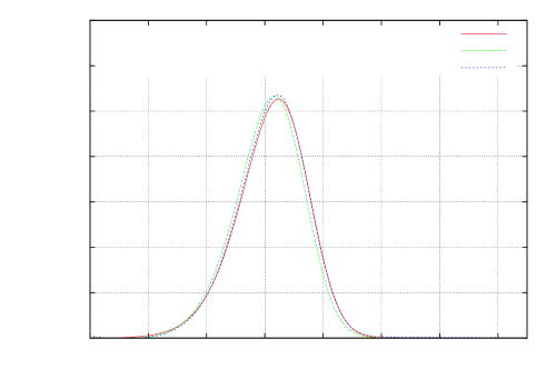
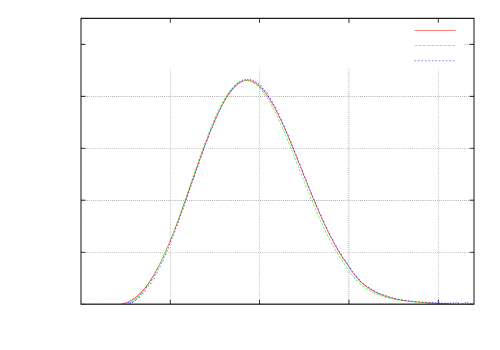
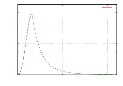
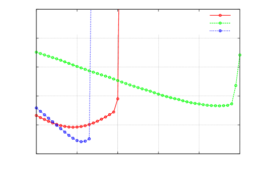
We measure the relative error in norm by
| (41) |
where is the exact numerical solution of the direct problem and represents the numerical reconstruction either by the Quasi-reversibility method or by the Filtering one. So we obtain for instance for the given parameters and the following reconstruction error of the division rate as a function of .
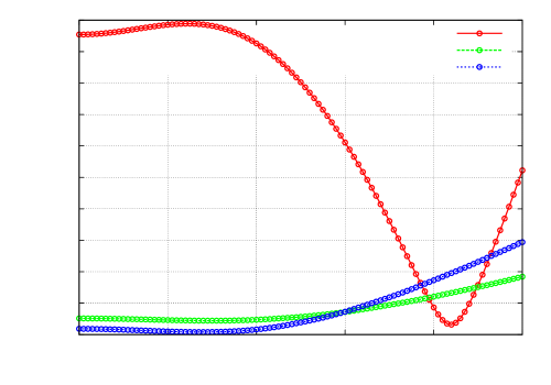
-
•
For the choice with
0 0.0002 0.0004 0.0006 0.0008 0.001 0.0012 0.0014 0.0016 0 5 10 15 20 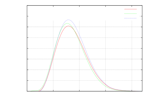
in D.P with in Quasi-rev: in Filtering: 0 0.0005 0.001 0.0015 0.002 0.0025 0.003 0.0035 0.004 0 5 10 15 20 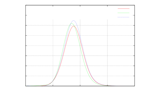
in D.P: in Quasi-rev: in Filtering: 0 0.002 0.004 0.006 0.008 0.01 0.012 0.014 0.016 0.018 0 2 4 6 8 10 12 14 16 18 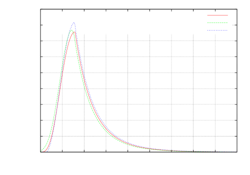
in D.P: in Quasi-rev: in Filtering: Figure 6: Numerical reconstruction of for each regularization method in the case . Top left:. Top right: . Down : . We measure the reconstruction error thanks to the relation (41) for the given parameters and we obtain the following representations
0.05 0.1 0.15 0.2 0.25 0.3 0 0.01 0.02 0.03 0.04 0.05 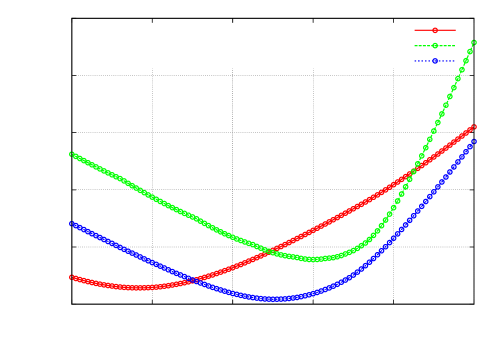
error for error for error for 0.02 0.04 0.06 0.08 0.1 0.12 0.14 0 0.01 0.02 0.03 0.04 0.05 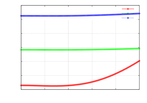
error for error for error for Figure 7: Numerical errors for with different choices of and in the direct problem. Left : errors by Quasi-reversibility method () . Right : errors by Filtering method.
4.2 Numerical reconstruction of in the noisy case
For this case, we consider as input data the values of the solution of the direct problem in which we add a multiplicative random noise uniformely distributed in (see [7] for a more precise statistical setting of noisy informations). The nonnegativity of the data is insured by the choice
Then with these noisy data we numerically obtain
-
•
For the case
0 0.0001 0.0002 0.0003 0.0004 0.0005 0.0006 0 2 4 6 8 10 12 14 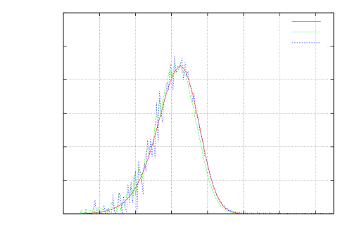
in D.P with Quasi-rev: Filtering: 0 0.0001 0.0002 0.0003 0.0004 0.0005 0.0006 0 2 4 6 8 10 12 14 16 18 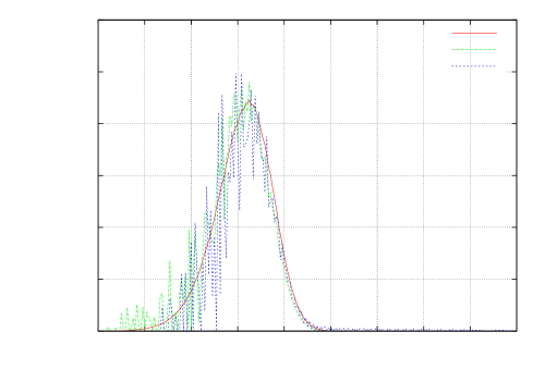
in D.P with Quasi-rev: Filtering: 0 0.0001 0.0002 0.0003 0.0004 0.0005 0.0006 0 2 4 6 8 10 12 14 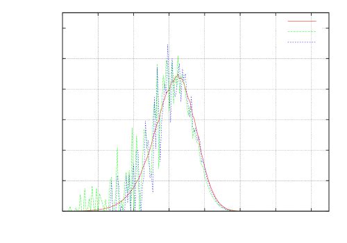
in D.P with Quasi-rev: Filtering: 0 0.0001 0.0002 0.0003 0.0004 0.0005 0.0006 0 2 4 6 8 10 12 14 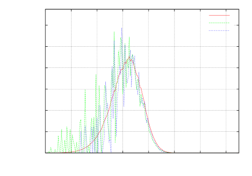
in D.P with Quasi-rev: Filtering: Figure 8: Numerical reconstruction of by the measured data for different values of with the choice , and . For various choice of the parameter we compute the relative error thanks to the relation (41) and obtain the following representations
0 0.1 0.2 0.3 0.4 0.5 0.6 0.7 0 0.01 0.02 0.03 0.04 0.05 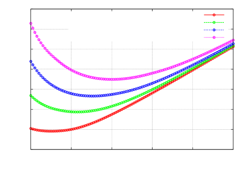
error for error for error for error for 0 0.2 0.4 0.6 0.8 1 0 0.01 0.02 0.03 0.04 0.05 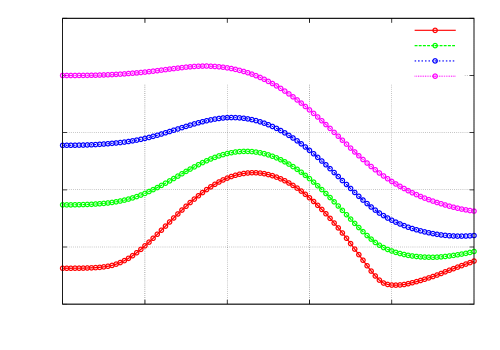
error for error for error for error for Figure 9: Numerical errors for different values of with , and in the direct problem. Left : errors by Quasi-reversibility method () . Right : errors by Filtering method.
Remark 2
Let us note that for data with high noise values the regularization by Quasi-reversibility method gives numerically better results than the Filtering one which creates big oscillations.
-
•
For the choice with
0 0.002 0.004 0.006 0.008 0.01 0.012 0.014 0.016 0.018 0 5 10 15 20 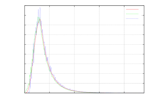
in D.P with Quasi-rev: Filtering: 0 0.005 0.01 0.015 0.02 0 5 10 15 20 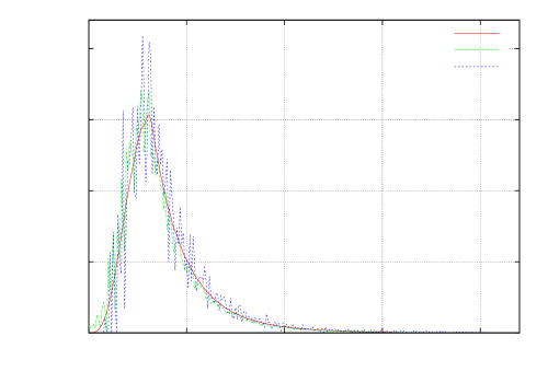
in D.P with Quasi-rev: Filtering: 0 0.005 0.01 0.015 0.02 0.025 0 5 10 15 20 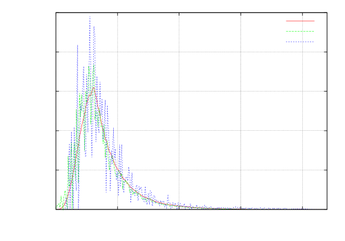
in D.P with Quasi-rev: Filtering: 0 0.005 0.01 0.015 0.02 0.025 0 5 10 15 20 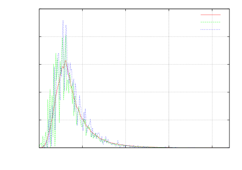
in D.P with Quasi-rev: Filtering: Figure 10: Numerical reconstruction of by the measured data for different values of with the choice , and . 0 0.2 0.4 0.6 0.8 1 0 0.005 0.01 0.015 0.02 0.025 0.03 0.035 0.04 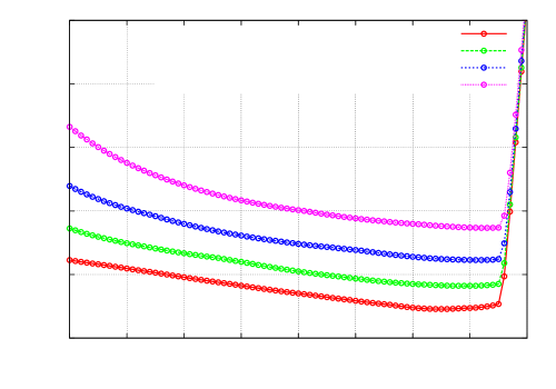
error for error for error for error for 0.2 0.3 0.4 0.5 0.6 0.7 0.8 0.9 0 0.02 0.04 0.06 0.08 0.1 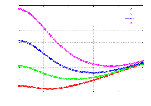
error for error for error for error for Figure 11: Numerical errors for different values of with , and in the direct problem. Left : errors by Quasi-reversibility method () . Right : errors by Filtering method.
Discussion
As shown by the numerical illustrations above, and after that we tried many different shapes of regularization (trying for instance a wide variety of and with in the quasi-reversibility method), our simulations still present some delicate points. Indeed, even if the regularization methods prove to give better result than the naive ”brute force” method as shown by Figure 9, the gain remains relatively small, and the regularizing parameter has also to remain small to avoid wrong reconstructions. Due to this small regularization, as shown by Figures 8, 10, the noise is filtered but not as much as we hoped first - especially for smaller that are farer from the departing point of the algorithm. Finally, the parameter needs to stay in a confidence interval, selected, for a given growth rate from a range of simulations carried out for various plausible birth rates (see for instance Figures 5, 7, 9).
5 Conclusion
We have addressed here the problem of recovering a birth rate of a size-structured population from measurements of the time-asymptotic profile of its density, in the general case when a given individual can give birth to two daughters of inequal sizes. Compared to the work carried out in [2, 3, 11] this last assumption has raised new difficulties, the principal one being that we have no other choice than considering the equation from the ”viewpoint” of the daughter cell - what implies to take into account the nonlocal integral term. We established theoretical estimates and built numerical methods to solve it. As shown above by our numerical illustrations however, some issues still remain to be solved, especially the behavior of the algorithm for smaller and the cancellations of oscillations (also present in [3, 11]).
References
- [1] Heinz W. Engl, Martin Hanke, and Andreas Neubauer. Regularization of inverse problems, volume 375 of Mathematics and its Applications. Kluwer Academic Publishers Group, Dordrecht, 1996.
- [2] Perthame, B., Zubelli, J. P (2007) . On the inverse problem for a size structured population model. Inverse Problem 23, 1037-1052.
- [3] Doumic, M., Perthame, B., Zubelli, J. P (2008) . Numerical Solution of an inverse problem in Size-Structured Population Dynamics.
- [4] Doumic, M. and Maia, P. and Zubelli, J.P., , On the Calibration of a Size-Structured Population Model from Experimental Data, Acta Biotheoretica, vol. 58(4), pp.405–13 (2010).
- [5] Doumic, M., Gabriel, P. (2010). Eigenelements of a General Aggregation-Fragmentation Model.
- [6] Brezis, H. Analyse Fonctionnelle et Applications.
- [7] Doumic, M., Hoffmann, M., Reynaud-Bouret, P. and Rivoirard, V., Nonparametric estimation of the division rate of a size-structured population, submitted.
- [8] Bekkal Brikci, F., Clairambault, J., Perthame, B. (2008). Analysis of a molecular structured population model with possible polynomial growth for the cell division cycle. Math. Comput. Modelling, 47(7-8):699-713.
- [9] Doumic, M. (2007). Analysis of a population model structured by the cells molecular content. Math. Model. Nat. Phenom., 2(3):121-152.
- [10] Calvez, V., Doumic, M., Gabriel, P. (2010). Self-similarity in a General Aggregation-fragmentation Problem; Application to Fitness Analysis. à paraitre.
- [11] Groh,A., Krebs, J. and Wagner, M., Efficient solution of an inverse problem in cell population dynamics, Inverse Problems, 27 (2011).
- [12] Metz, J. A. J. and Diekmann, O. The dynamics of physiologically structured populations, Lecture Notes in Biomathematics, vol. 68, Springer-Verlag (1986).
- [13] Perthame, B. (2007). Transport equations in biology. Frontiers in Mathematics. Birkhäuser Verlag, Basel.
- [14] Pherthame, B., Ryzhik, L. (2005). Exponential decayfor the fragmentation or cell-division equation. J. Differential Equations, 210(1):155-177.
- [15] Michel, P., Mischler, Perthame, B. (2005). General entropy equations for structured population models and scattering. C. R. Math. Acad. Sci. Paris, 338(9):697-702.
- [16] Baumeister, J., Leitão, A. (2005). Topics in Inverse Problems, 25, Brazilian Mathematics Coll. (Rio de Janeiro: IMPA Mathematical Publications).
- [17] Lattès, R., Lions, J-L. (1967). Méthode de quasi-réversibilité et applications. Travaux et Recherches Mathématiques no 15, Paris: Dunod.