Environment-Assisted Error Correction of Single-Qubit Phase Damping

Abstract

Open quantum system dynamics of random unitary type may in principle be fully undone. Closely following the scheme of environment-assisted error correction proposed by Gregoratti and Werner [M. Gregoratti and R. F. Werner, J. Mod. Opt. 50 (6), 915–933 (2003)], we explicitly carry out all steps needed to invert a phase-damping error on a single qubit. Furthermore, we extend the scheme to a mixed-state environment. Surprisingly, we find cases for which the uncorrected state is closer to the desired state than any of the corrected ones.

I Introduction

Coherent superpositions of quantum states lay the foundation for genuinely non-classical phenomena such as entanglement or interference of massive particles. With growing system size these superpositions become however increasingly fragile, thereby impeding future realizations of quantum technology. The interaction of the system of interest with its surroundings leads to a loss of the interference potential—a process usually denoted with decoherence Joos2002 . Phase damping (a.k.a. dephasing) denotes the case of pure decoherence. Here, the populations remain unaffected; rather, only the coherences itself (i.e., the off-diagonal elements of the density matrix) are subject to decay. This discrimination of decoherence against pure decoherence may for example be adequate in situations where the characteristic time describing polarization decay is much smaller than the typical dissipation time Braun:2001p2029 .

Arguably, one may identify two main mechanisms responsible for decoherence. The first and most prominent approach rests on the language of open quantum systems Zurek2003 ; Schlosshauer2007 . Here, the system of interest is seen as being part of a larger (often infinite) quantum system, where also the environmental degrees of freedom are incorporated. The decoherence is then a direct consequence of growing correlations between system and environment. It is worth noting that these correlations are not necessarily of quantum nature: the system may in fact decohere completely without being entangled to its surroundings at all EisertPlenio2002 ; PerniceStrunz2011 . As a second relevant source of decoherence one may consider stochastic fluctuations of ambient fields (or “random external fields” Nielsen_Chuang_2007 ; AlickiLendi1987 ). In fact, fluctuating fields were successfully identified as the main source of decoherence in ion trap quantum computers, where fluctuations are present both in the trapping field and in the lasers addressing the individual ions Monz:2010p3941 . This ensemble-based approach may be described in terms of a stochastic Schrödinger equation, where time evolution is unitary, yet stochastic. Usually, dynamics of this type is denoted random unitary (RU).

In this context it is sometimes argued that the latter mechanism should be merely seen as a fake decoherence process. The argument is partly based on the idea that, due to the unitary character of time evolution for individual members of the ensemble, the dynamics is in principle reversible Zurek2003 ; Schlosshauer2007 (the spin echo technique, for example, is based on this idea). However, it is known that genuine open quantum system dynamics may be reversible, too, provided the reduced dynamics is RU and thus indistinguishable from the dynamics caused by fluctuating fields gregoratti2003quantum . Here, the actual correction procedure is conditional on classical information obtained from a measurement performed on the system’s quantum environment. It thus represents an instance of environment-assisted error correction. In principle, any phase damping of a single qubit or qutrit may be corrected this way, since the dynamics is always of RU type LandauStreater1993 ; BuscemiDAriano2005 .

The present article provides a thorough assessment of all the steps involved in a complete reversal of a given phase-damping dynamics on a single qubit. In Sec. II we discuss the basic tools needed for the environment-assisted error correction of RU dynamics. The scheme is then applied in Sec. III to the example of single-qubit phase damping. In addition to the original scheme, where the environment is assumed to be in a pure state initially, we study a possible extension of the correction scheme in case of a mixed-state environment (Sec. IV).

II Environment-assisted error correction

In the theory of quantum error correction one usually assumes that there is a certain (low) probability for an error acting locally on qubits or gates. Furthermore it is assumed that one needs to account for different kinds of errors represented by a certain set of error operations. The probabilities for different errors to occur are independent of each other and given a priori Gottesman:1997zz . The correction mechanisms are designed such that they can detect and correct all errors from the set of possible error operations. This requires an encoding of the logical qubits used for the actual computation into a larger number of physical qubits as can be nicely seen in the Shor code picture Shor1995 . In addition, the realization of a unitary gate in the algorithm requires a translation into a set of unitaries acting on the physical qubits. The whole process is described by the beautiful theory of fault tolerant quantum computation Nielsen_Chuang_2007 . Unfortunately as pointed out in, e.g.Gottesman:1997zz , the scaling of the number of physical qubits is, though only polylogarithmic in the asymptotic limit, too severe even for a very small number of computational qubits to permit an experimental realization by current means. Sometimes, being able to perform measurements on the environment of the qubits allows to recover quantum states. As an example, in Alber2001 a continuous monitoring of the decay processes provides the information for a conditional recovery operation.

Environment-assisted error correction as proposed in gregoratti2003quantum is a different approach to quantum error correction. Here, the correction is based on classical information obtained from a measurement on the system’s environment. The scheme allows for a complete correction of RU dynamics, provided the (quantum) environment is initially in a pure state. We closely follow the ideas presented in gregoratti2003quantum ; we are, however, interested in carrying out the procedure lined out in the aforementioned work for a feasible realization of an open quantum system. In the following we will present a scheme that allows the explicit construction of an observable for such a measurement. Our results will provide a correction scheme for a phase-damping interaction between a qubit and an initially pure environment of finite dimension.

II.1 Quantum channels

In the context of open quantum systems, a quantum channel describes the time-evolution of a quantum system arising from the joint unitary evolution of system plus environment. Under the usual assumption of vanishing initial correlations, system and environment are initially described by a product state $\rho\otimes\rho_{E}$. The channel is then obtained by tracing out the environmental degrees of freedom

$$\Phi(\rho)=\mathrm{tr}_{E}\left(e^{-\mathrm{iH}t}\rho\otimes\rho_{E}e^{\mathrm{iH}t}\right).$$ (1)

The total Hamiltonian $\mathrm{H}$ includes the interaction between system and environment. According to Kraus1969 ; Kraus1970 , every such channel has a nonunique decomposition

$$\rho^{\prime}:=\Phi(\rho)=\sum_{\alpha}\mathrm{K}_{\alpha}\rho\mathrm{K}^{\dagger}_{\alpha}=\sum_{\beta}\mathrm{L}_{\beta}\rho\mathrm{L}^{\dagger}_{\beta},$$ (2)

where two corresponding sets of so-called Kraus operators $K_{\alpha},L_{\beta}$ are related via a unitary matrix $\mathrm{V}=\left(v_{\alpha\beta}\right)$ choi1975 , so that

$$\mathrm{K}_{\alpha}=\sum_{\beta}v_{\alpha\beta}\mathrm{L}_{\beta}.$$ (3)

In case of RU dynamics it is possible to find a decomposition of the channel into unitary operators,

$$\Phi_{\mathrm{RU}}(\rho)=\sum_{\alpha}p_{\alpha}\mathrm{U}_{\alpha}\rho\mathrm{U}_{\alpha}^{\dagger},$$ (4)

where $p_{\alpha}>0,\sum_{\alpha}p_{\alpha}=1$. The Kraus operators are thus unitary up to normalization, $K_{\alpha}=\sqrt{p_{\alpha}}U_{\alpha}$. Obviously, a RU channel is unital, that is, leaving the completely mixed state invariant, $\Phi_{\mathrm{RU}}(\mathds{1})=\mathds{1}$.

Phase damping (or dephasing) is the case of pure decoherence, where, in a fixed basis $\{|n\rangle\}$ (the phase-damping basis), no population transfer occurs. According to this basis of “preferred states”, the projectors are constants of the motion. In such a case the Hamiltonian describing the system-environment coupling may be diagonalized with respect to the phase-damping basis: $\mathrm{H}=\sum_{n}|n\rangle\!\langle n|\otimes\mathrm{h}_{n}$ GorinStrunz2004 . Here, the relative Hamiltonians $\mathrm{h}_{n}$ act on the environment, only. Assuming the environment to start in a pure state, $|\psi_{0}\rangle$, the phase-damping dynamics is fully described in terms of the overlap of the relative states $|\psi_{n}\rangle:=e^{-i\mathrm{h}_{n}t}|\psi_{0}\rangle$, that is

$$\rho_{mn}^{\prime}=\langle\psi_{n}|\psi_{m}\rangle\;\rho_{mn}.$$ (5)

Leaving the diagonal elements intact, phase-damping channels are unital by definition. In their article LandauStreater1993 Landau and Streater show that a phase-damping channel acting on a single qubit or qutrit may always be decomposed into a RU decomposition, Eq. (4). In principle, phase-damping errors on systems of dimension $2$ or $3$ may thus be completely undone.

II.2 The correction scheme

If the initial state of the environment is pure, $\rho_{E}=|\psi_{0}\rangle\!\langle\psi_{0}|$, a certain Kraus decomposition is selected by choosing a basis $\{|\chi_{\beta}\rangle\}_{\beta}$ of $\mathcal{H}_{E}$. Upon insertion into Eq. (1), this leads to

$$\Phi(\rho) = \sum_{\beta}\langle\chi_{\beta}|e^{-\mathrm{iH}t}|\psi_{0}\rangle\rho\langle\psi_{0}|e^{\mathrm{iH}t}|\chi_{\beta}\rangle$$ (6)

$$= \sum_{\beta}L_{\beta}\rho L_{\beta}^{\dagger},$$

where we identify $\mathrm{L}_{\beta}=\langle\chi_{\beta}|e^{-\mathrm{iH}t}|\psi_{0}\rangle$.

In principle, this identification allows to select the dynamics where only a single term of the operator sum (2) applies:

$$\mathrm{L}_{\beta}\rho\mathrm{L}^{\dagger}_{\beta}=\mathrm{tr}_{E}\left(e^{-\mathrm{iH}t}\rho\otimes\rho_{E}e^{\mathrm{iH}t}(\mathds{1}\otimes\mathrm{P}_{\beta})\right),$$ (7)

with the projector $\mathrm{P}_{\beta}=|\chi_{\beta}\rangle\!\langle\chi_{\beta}|$. The unitary equivalence between different decompositions allows to write $\mathrm{K}_{\alpha}=\langle\mu_{\alpha}|e^{-\mathrm{iH}t}|\psi_{0}\rangle$ with $|\mu_{\alpha}\rangle=\sum_{\beta}\mathrm{V}_{\alpha\beta}|\chi_{\beta}\rangle$.

The principle of correction of a RU channel $\Phi_{RU}$ is now straightforward: it relies on the identification of an appropriate basis $|\mu_{\alpha}\rangle$ corresponding to a RU decomposition of the channel. The projectors $\mathrm{Q}_{\alpha}=|\mu_{\alpha}\rangle\!\langle\mu_{\alpha}|$ may then be used to single out the subnormalized sub-state

$$\rho^{\prime}_{\alpha}=p_{\alpha}\mathrm{U}_{\alpha}\rho\mathrm{U}^{\dagger}_{\alpha}=\mathrm{tr}_{E}\left(e^{-\mathrm{iH}t}\rho\otimes\rho_{E}e^{\mathrm{iH}t}(\mathds{1}\otimes\mathrm{Q}_{\alpha})\right),$$

which, upon normalization, is unitarily related to the initial state $\rho$.

For a suitable observable $\mathrm{O}$ on $\mathcal{H}_{E}$ with projectors on non-degenerate eigenspaces, $\mathrm{O}=\sum_{\alpha}\lambda_{\alpha}\mathrm{Q}_{\alpha}$ with $\mbox{tr}(\mathrm{Q}_{\alpha}\mathrm{Q}_{\beta})=\delta_{\alpha\beta}\mathrm{Q}_{\alpha}$, a measurement outcome of $\lambda_{\alpha}$ allows to unambiguously discriminate between sub-states $\rho^{\prime}_{\alpha}$. The perfect recovery of the initial state is achieved by $\mathrm{U}^{\dagger}_{\alpha}\rho_{\alpha}\mathrm{U}_{\alpha}$. Gregoratti and Werner show in gregoratti2003quantum that RU channels are the only ones thus allowing for a perfect correction.

III Explicit implementation: Correction of single qubit phase damping

In practice, the correction scheme faces several impediments. First of all, no simple method is known how to decide whether a given channel has a RU decomposition. Second, even if such a decomposition is possible, the single unitaries $\mathrm{U}_{\alpha}$ have to be known in detail. Once these hurdles are overcome, one has to find explicit expressions for all $\mathrm{Q}_{\alpha}$. The realization of this last step is discussed in the original formulation gregoratti2003quantum . Here, the unitary equivalence between equivalent Kraus decompositions, Eq. (3), plays a central role.

Now we have all ingredients to construct a Hamiltonian generating a RU channel on a qubit and to proceed with the construction of the observable. For a phase-damping channel on a qubit there are only two relative Hamiltonians $\mathrm{h}_{1}$, $\mathrm{h}_{2}$ leading to the relative states $|\psi_{1}(t)\rangle=e^{-\mathrm{ih_{1}}t}|\psi_{0}\rangle$, $|\psi_{2}(t)\rangle=e^{-\mathrm{ih_{2}}t}|\psi_{0}\rangle$ on the environment. The action of the phase-damping channel has a very simple form in terms of their overlap, $C(t):=\langle\psi_{2}(t)|\psi_{1}(t)\rangle$,

$$\rho^{\prime}=\left(\begin{array}[]{cc}\rho_{11}&C\rho_{12}\\ \bar{C}\rho_{21}&\rho_{22}\end{array}\right).$$ (8)

We have suppressed the time dependence in the equation above and will from now on only consider quantities for a fixed value of $t$. We have already seen that using the basis $\{|\chi_{\beta}\rangle\}_{\beta}$ of $\mathcal{H}_{E}$ to explicitly perform the trace allows us to identify $\mathrm{L}_{\beta}=\langle\chi_{\beta}|e^{-\mathrm{iH}t}|\psi_{0}\rangle$ so that we can write

$$\mathrm{L}_{\beta}=\left(\begin{array}[]{cc}\langle\chi_{\beta}|\psi_{1}\rangle&0\\ 0&\langle\chi_{\beta}|\psi_{2}\rangle\end{array}\right).$$ (11)

III.1 RU decomposition

In order to obtain the RU decomposition we compute the dynamical or Choi matrix of our phase-damping channel. For $n=\mathrm{dim}\mathcal{H}_{S}$, $\Phi:\mathcal{H}_{S}\rightarrow\mathcal{H}_{S}$ we can identify $\mathcal{H}_{S}\sim\mathds{C}^{n}$ and the Choi matrix is defined as the $n^{2}\times n^{2}$ matrix containing the action of $\Phi$ on all $n\times n$ matrices $\mathrm{E}_{ij}=\mathbf{e}_{i}^{T}\mathbf{e}_{j}$ that form a basis of $\mathcal{M}(n\times n,\mathds{C})$,

$$\left(\begin{array}[]{cc}\Phi\left(\begin{array}[]{cc}1&0\\ 0&0\end{array}\right)&\Phi\left(\begin{array}[]{cc}0&1\\ 0&0\end{array}\right)\\ \Phi\left(\begin{array}[]{cc}0&0\\ 1&0\end{array}\right)&\Phi\left(\begin{array}[]{cc}0&0\\ 0&1\end{array}\right)\end{array}\right)=\left(\begin{array}[]{cccc}1&0&0&C\\ 0&0&0&0\\ 0&0&0&0\\ \bar{C}&0&0&1\end{array}\right).$$ (12)

Diagonalization of this $4\times 4$ matrix yields the nonzero eigenvalues

• $\lambda_{1}=1-|C|$: $\mathbf{v}_{\lambda_{1}}=\frac{1}{\sqrt{2}}(-\frac{C}{|C|},0,0,1)^{T}$

• $\lambda_{2}=1+|C|$: $\mathbf{v}_{\lambda_{2}}=\frac{1}{\sqrt{2}}(\frac{C}{|C|},0,0,1)^{T}$

with corresponding eigenvectors $\mathbf{v}_{\lambda_{1}},\mathbf{v}_{\lambda_{2}}$. According to a central result in choi1975 we can obtain Kraus operators by rearranging the eigenvectors of the above Choi matrix into $2\times 2$ matrices, resulting in the decomposition

$$\rho^{\prime} = \frac{1-|C|}{2}\left(\begin{array}[]{cc}-\frac{C}{|C|}&0\\ 0&1\end{array}\right)\rho\left(\begin{array}[]{cc}-\frac{C^{*}}{|C|}&0\\ 0&1\end{array}\right)$$

$$+\frac{1+|C|}{2}\left(\begin{array}[]{cc}\frac{C}{|C|}&0\\ 0&1\end{array}\right)\rho\left(\begin{array}[]{cc}\frac{C^{*}}{|C|}&0\\ 0&1\end{array}\right)$$

$$=: \sum\limits_{\alpha=1}^{2}K_{\alpha}\rho K_{\alpha}^{\dagger}.$$

Note that the Kraus operators of the decomposition in (III.1) are trivially unitary up to a scaling factor, $K_{\alpha}K_{\alpha}^{\dagger}=K_{\alpha}^{\dagger}K_{\alpha}=p_{\alpha}\mathds{1},\alpha=1,2$. It is easily verified that this RU decomposition recovers Eq. (8).

III.2 Finding the correction observable

Consider now the situation where the actual environment is of dimension $n$. As a consequence the set $\{\mathrm{L}_{\beta}\}_{\beta}$ contains $n$ elements and according to Eq. (3) we know that there exists a unitary matrix $\mathrm{V}$ that relates $\{\mathrm{L}_{\beta}\}_{\beta}$ to the RU decomposition $\{\mathrm{K}_{\alpha}\}_{\alpha}$ in (III.1), if the latter is extended by $n-2$ zero matrices $\mathrm{K}_{\alpha}=\sqrt{p}_{\alpha}\mathrm{U}_{\alpha}$, $\alpha=1,2$, $\mathrm{K}_{\alpha}=0_{(2)}$, $\alpha=3,\dots,n$. We will now show in detail how it is possible to obtain $\mathrm{V}$ from the two sets of Kraus operators $\{\mathrm{K}_{\alpha}\}_{\alpha}$ and $\{\mathrm{L}_{\beta}\}_{\beta}$. Due to their diagonal character the Kraus operators may be rewritten in terms of vectors $K_{\alpha}=(K^{\alpha}_{11},K^{\alpha}_{22})$. The unitary equivalence, Eq. (3), thus translates to the following linear system for the rows $\mathbf{v}_{\alpha}$ of $\mathrm{V}$,

$$\left(\begin{array}[]{c}K^{\alpha}_{1}\\ K^{\alpha}_{2}\end{array}\right)=\left(\begin{array}[]{cccc}L^{1}_{1}&L^{2}_{1}&\dots&L^{n}_{1}\\ L^{1}_{2}&L^{2}_{2}&\dots&L^{n}_{2}\end{array}\right)\left(\begin{array}[]{c}v_{\alpha 1}\\ v_{\alpha 2}\\ \vdots\\ v_{\alpha n}\end{array}\right),$$ (22)

where in addition all double indices are suppressed. For $\alpha=1,2$ (22) is an inhomogeneous system $\mathrm{A}\mathbf{v}_{\alpha}=\mathbf{b}_{\alpha}$ with inhomogeneities obtained from $\mathrm{K}_{1}$, $\mathrm{K}_{2}$ given by

$$\mathbf{b}_{1} =\sqrt{\frac{1-|C|}{2}}\left(\begin{array}[]{c}-\frac{C}{|C|}\\ 1\end{array}\right)$$ (25)

$$\mathbf{b}_{2} =\sqrt{\frac{1+|C|}{2}}\left(\begin{array}[]{c}\frac{C}{|C|}\\ 1\end{array}\right).$$ (28)

For $\alpha=3,\dots,n$ one has to fulfill the homogeneous system $\mathrm{A}\mathbf{v}_{\alpha}=0$. In addition, unitarity of $\mathrm{V}$ requires that $\langle\mathrm{v}_{\alpha}|\mathrm{v}_{\beta}\rangle=\delta_{\alpha\beta}$. In other words we need to find $n-2$ orthonormal vectors $\mathbf{v}_{\alpha}\,\in\,\mathrm{ker}(\mathrm{A})$ and two orthonormal vectors $\mathbf{v}_{\alpha}\,\in\,\mathrm{ker}(\mathrm{A})^{\perp}$ satisfying the inhomogeneous equations. In the following we will show that the singular value decomposition of $\mathrm{A}$ will provide all of the required solutions $\mathbf{v}_{\alpha}$.

The $2\times n$ matrix $\mathrm{A}$ has singular value decomposition $\mathrm{A}=\mathrm{U}\Sigma\mathrm{W}^{\dagger}$, with $\mathrm{U}$ a unitary $2\times 2$ matrix with columns spanning $\mathrm{im(A)}$, $\Sigma$ a $2\times n$ diagonal matrix containing the singular values $\lambda_{i}$ of $\mathrm{A}$, and $\mathrm{W}$ a $n\times n$ unitary matrix. If $r=\mathrm{rank(A)}$, the first $r$ columns of $\mathrm{W}$ form an ONB of $\mathrm{ker(M)}^{\perp}$ and the last $n-r$ columns form an ONB of $\mathrm{ker(A)}$. Using the completeness relation $\sum_{\beta=1}^{n}|\chi_{\beta}\rangle\!\langle\chi_{\beta}|=\mathds{1}$ it is straightforward to show that $\mathrm{A}\mathrm{A}^{\dagger}=\left(\begin{array}[]{cc}1&C\\ \bar{C}&1\end{array}\right)=\mathrm{U}(\Sigma\Sigma^{\dagger})\mathrm{U}^{\dagger}$. Diagonalizing $\mathrm{A}\mathrm{A}^{\dagger}$ results in $\mathrm{A}\mathrm{A}^{\dagger}=U\left(\begin{array}[]{cc}1-|C|&0\\ 0&1+|C|\end{array}\right)U^{\dagger}$, with eigenvectors $\mathbf{u}_{1}=\frac{1}{\sqrt{2}}\left(\begin{array}[]{c}-\frac{C}{|C|}\\ 1\end{array}\right)$, $\mathbf{u}_{2}=\frac{1}{\sqrt{2}}\left(\begin{array}[]{c}\frac{C}{|C|}\\ 1\end{array}\right)$ forming the columns of $\mathrm{U}$. The singular values of $\mathrm{A}$ can be read off as the square root of the eigenvalues of $\mathrm{A}\mathrm{A}^{\dagger}$, $\lambda_{1}=\sqrt{1-|C|}$ and $\lambda_{2}=\sqrt{1+|C|}$. Now let $\mathbf{w}_{i}$ be the columns of $\mathrm{W}$. Using the singular value decomposition of $\mathrm{A}$ it is now obvious that $\mathrm{A}\mathbf{w}_{1}=\lambda_{1}\mathbf{u}_{1}=\mathbf{b}_{1}$, $\mathrm{A}\mathbf{w}_{2}=\lambda_{2}\mathbf{u}_{2}=\mathbf{b}_{2}$ and $\mathrm{A}\mathbf{w}_{i}=0$ for all $i=3,\dots,n$. This means that the singular value decomposition of $\mathrm{A}$ provides the desired solutions $\mathbf{v}_{\alpha}$ to the linear system (22) via the columns $\mathbf{w}_{i}$ of the unitary matrix $\mathrm{W}$. Thus we can finally conclude that the unitary matrix $\mathrm{V}$ relating the RU decomposition of $\Phi_{D}$ to the decomposition with respect to the basis $\{|\chi\rangle_{\beta}\}_{\beta}$ is given by

$$\mathrm{V}=\mathrm{W}^{T}.$$

We can transform the basis $\{|\chi\rangle_{\beta}\}_{\beta}$ to the desired measurement basis $\{|\mu_{\alpha}\rangle\}_{\alpha}$ via

$$|\mu_{\alpha}\rangle=\sum_{\beta}(\mathrm{W}^{\dagger})_{\alpha\beta}|\chi_{\beta}\rangle.$$

The projectors $\mathrm{Q}_{\alpha}$ for the observable $\mathrm{O}$ on $\mathcal{H}_{E}$ are given by $\mathrm{Q}_{\alpha}=|\mu_{\alpha}\rangle\!\langle\mu_{\alpha}|$.

Now the general correction scheme consists of the following steps: i) Performe a measurement on the environment using the observable $\mathrm{O}=\sum_{\alpha=1}^{n}\lambda_{\alpha}\mathrm{Q}_{\alpha}$, with $\lambda_{1}\neq\lambda_{2}$ resulting in a post measurement state $\rho_{\alpha}=\mathrm{U}_{\alpha}\rho\mathrm{U}^{\dagger}_{\alpha}$ for all possible measurement outcomes $\lambda_{\alpha}$. ii) Apply the unitary transformation $\mathrm{U}^{\dagger}_{\alpha}\rho_{\alpha}\mathrm{U}_{\alpha}$ conditional on the outcome of the measurement of $\mathrm{O}$. The probability to get $\lambda_{\alpha}$ is $p(\lambda_{\alpha})=p_{\alpha}$, $\alpha=1,2$ and $p(\lambda_{\alpha})=0$ otherwise.

The following sequence of figures intends to provide further insight into the mechanism of the correction scheme. For simplicity we consider a two dimensional environment so that we can represent state vectors of system and environment in the Bloch-sphere picture. Fig. 1 (a) shows a sequence of phase-damping channels $\Phi_{t}$ acting on the pure initial system state $\rho$. The adjacent Fig. 1 (b) displays the corrected state for each of the states $\Phi_{t}(\rho)$ after a measurement of the correction observable $O$ (which in general will be different for different channels $\Phi_{t}$) and the application of the correction procedure $R_{\alpha}$ (which depends on the measurement outcome $\alpha$ as well as the channel $\Phi_{t}$). The correction procedure recovers the initial state $\rho$ for each channel $\Phi_{t}$. One can think of the combined action of measurement and correction procedure as the process that mediates between Fig. 1 (a) and (b).

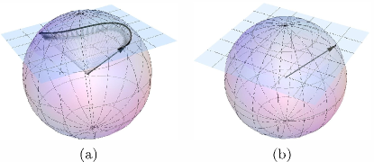
Figure 1: (Color Online) Phase-damping and correction for an initially pure environment. (a) The pure initial state $\rho$ of the system (black arrow) is mapped to a mixed state $\Phi_{t}(\rho)$ (thick, black line). The phase-damping interaction leaves invariant the $z$-value of the Bloch vector (the time-evolved states lie on a plane of constant $z$). (b) The corrected state $\tilde{\rho}=R_{\alpha}(\rho_{\alpha})$ after a measurement of $\mathrm{O}$ with outcome $\lambda_{\alpha}$ and application of the appropriate correcting channel $R_{\alpha}$. The corrected state $\tilde{\rho}$ is identical to the initial state $\rho$ of (a) for all of the above channels $\Phi_{t}$.

The phase-damping channel $\Phi_{t}$ is completely determined by the two relative states $|\psi_{1}(t)\rangle$, $|\psi_{2}(t)\rangle$. Their unitary time evolution is displayed in Fig. 2 (a). The states $|\mu\rangle_{\alpha}$ spanning the eigenspaces of the correction observable $\mathrm{O}$ do also depend on the time parameter $t$ labeling the different phase damping channels $\Phi_{t}$. Their time-evolution is displayed in Fig. 2 (b).

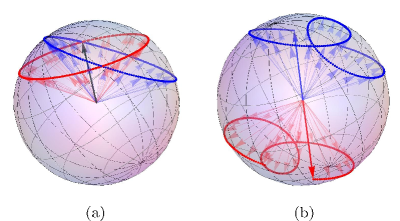
Figure 2: (Color online) (a) Unitary evolution of the relative states $|\psi_{1}(t)\rangle$ (red) and $|\psi_{2}(t)\rangle$ (blue). The initial state $|\psi_{0}\rangle$ is indicated by the black arrow lying on the intersection of the cones. (b) Correction observables $\mathrm{E}_{1}$ (red) and $\mathrm{E}_{2}$ (blue) for different channels $\Phi_{t}$. The two observables span orthogonal subspaces of $\mathcal{H}_{E}$ (the corresponding Bloch vectors point to opposite points).

IV Mixed environments

Until now it was assumed that the environment is initially in the pure state $|\psi_{0}\rangle$. In this section we want to investigate the case of a mixed-state environment. We apply modified versions of the correction scheme for pure environments and explicitly show that none of these protocols leads to a satisfying correction of the phase-damping channel. For a mixed environment there is no unique correspondence between the projection $\mathrm{Q}_{\alpha}$ on the environment Hilbert space and a single Kraus operator $\mathrm{K}_{\alpha}$ as in the case of a pure initial environment. We assume that our environment is two-dimensional and that its initial state is given by the mixture $\rho_{E}=w|\psi_{0}\rangle\!\langle\psi_{0}|+(1-w)|\psi^{\perp}_{0}\rangle\!\langle\psi^{\perp}_{0}|$. For concreteness think of a low but not zero temperature environment such that $w$ is less but close to $1$. The coupling is realized via the following Hamiltonian, $\mathrm{H}=k\sigma_{z}^{S}\otimes\sigma_{z}^{E}+\mathds{1}\otimes\mathbf{\Gamma}\mathbf{\sigma}$, $\sigma=\sum_{i=1}^{3}\sigma_{i}\mathbf{e}_{i}$ the vector of Pauli-spin matrices and $\mathbf{\Gamma}\in\mathds{R}^{3}$. The Hamiltonian can be written as $\sum_{i=1,2}|s_{z}^{i}\rangle\!\langle s_{z}^{i}|\otimes\mathrm{h}_{i}$, where $|s_{z}^{i}\rangle$ are the eigenstates of $\sigma_{z}^{S}$ and $\mathrm{h}_{1}=k\sigma_{z}^{E}+\mathbf{\Gamma}\sigma^{E}$, $\mathrm{h}_{2}=-k\sigma_{z}^{E}+\mathbf{\Gamma}\sigma^{E}$. The channel $\Phi$ generated by $\mathrm{H}$ according to Eq. (1) preserves the diagonal elements of $\rho$ in the $|s_{z}^{i}\rangle$ basis. For $\rho_{E}$ mixed the phase-damping interaction generates two additional relative states $|\psi^{\perp}_{1}\rangle=e^{-\mathrm{ih_{1}}t}|\psi^{\perp}_{0}\rangle$ and $|\psi^{\perp}_{2}\rangle=e^{-\mathrm{ih_{2}}t}|\psi^{\perp}_{0}\rangle$ in $\mathcal{H}_{E}$. The action of $\Phi$ is similar to the pure case, Eq. (8), but $C$ is replaced by $wC+(1-w)C^{\perp}$. $C^{\perp}$ is again given by an overlap of relative states, $C^{\perp}=\langle\psi^{\perp}_{2}|\psi^{\perp}_{1}\rangle$.

IV.1 Correction schemes for mixed environments

In order to perform a correction we treat the channel as if it was generated by the pure initial environment state $|\psi_{0}\rangle$ (or $|\psi^{\perp}_{0}\rangle$). For $|\psi_{0}\rangle$ we calculate the corresponding projectors $\mathrm{Q}_{1}$, $\mathrm{Q}_{2}$, the observable $\mathrm{O}=\sum_{i=1,2}\lambda_{i}\mathrm{Q}_{i}$, $\lambda_{1}\neq\lambda_{2}$, for a measurement on the environment, probabilities $p(\lambda_{1})$, $p(\lambda_{2})$ of the RU decomposition and unitary operators $\mathrm{U}_{1}$, $\mathrm{U}_{2}$ for the correction operation. We will call the states resulting from this correction procedure $\rho_{\alpha,c}$. Similarly for $|\psi^{\perp}_{0}\rangle$ we calculate $\mathrm{P}_{1}$, $\mathrm{P}_{2}$, $\mathrm{O}^{\perp}=\sum_{i=1,2}\mu_{i}\mathrm{P}_{i}$, $\mu_{1}\neq\mu_{2}$, $r_{1}$, $r_{2}$ and $\mathrm{V}_{1}$, $\mathrm{V}_{2}$ and call the corrected states $\sigma_{\alpha,c}$ (the possible correction pathways for a mixed state are displayed in Fig. 3). A measurement of $\mathrm{O}$ ($\mathrm{O}^{\perp}$) and a successive outcome dependent correction $\mathrm{U}_{i}$ ($\mathrm{V}_{i}$) will not perfectly correct $\Phi$ since we have neglected the fact that $\rho_{E}$ is a mixture.

Figure 3: Schematic picture of the possible correction schemes for a mixed environment (see text for details).

Several correction protocols can be considered. First, the corrector might simply ignore the fact that there is a small admixture of $|\psi^{\perp}_{0}\rangle$. In this case, the state after correction is given by $p(\lambda_{1})\rho_{1,c}+p(\lambda_{2})\rho_{2,c}=:\rho_{c}$. Second, as a matter of keeping an open mind the corrector might want to mirror the mixed-state probabilities for the two states in his choice of correction scheme. In other words, he performs the measurement on $\mathcal{H}_{E}$ and the successive correction with a probability of $w$ as if $\rho_{E}$ was the pure state $|\psi_{0}\rangle$ and with a probability of $1-w$ as if $\rho_{E}$ was $|\psi^{\perp}_{0}\rangle$. We call the state resulting from an ensemble average over states corrected in this manner $\tilde{\rho}_{c}=w\rho_{c}+(1-w)\sigma_{c}$.

IV.2 The error of the correction

In order to quantify the quality of the correction we measure the distance between the corrected states $\rho_{\alpha,c}$, $\sigma_{\alpha,c}$, $\rho_{c}$, and $\tilde{\rho}_{c}$ and the initial state $\rho$, and compare it to the distance between the uncorrected state $\Phi(\rho)$ and the initial state. The trace norm Nielsen_Chuang_2007 , $\lVert\rho\rVert=\frac{1}{2}\mbox{tr}\sqrt{\rho^{\dagger}\rho}$, is a suitable distance measure in the set of states that will later allow us to derive strict bounds analytically. In Fig. 4 we show results of the correction protocol for a small admixture of $|\psi^{\perp}_{0}\rangle$ to $|\psi_{0}\rangle$ in $\rho_{E}$ ($w=0.9$). Clearly, applying any of the correction procedures does not necessarily lead to an improvement. Indeed, we can see that even for a small admixture there are phase-damping channels $\Phi_{t}$ (corresponding to interaction times $t$) for which the uncorrected state is closer to the desired state than any of the corrected ones.

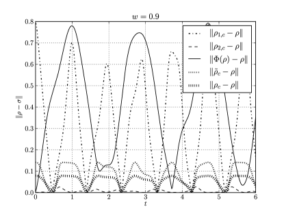
Figure 4: Trace distance as a measure for the quality of the corrected state. Different channels $\Phi_{t}$ arising from $\mathrm{H}$ and an initial state $\rho_{E}$ containing a small admixture of $|\psi_{0}^{\perp}\rangle$ ($w=0.9$) are corrected using the correction scheme for pure states (details see text). Clearly, there are cases where the uncorrected state $\Phi_{t}(\rho)$ (solid line) is closer to the desired state than the results from any of the correction schemes.

We observe from Fig. that the correction scheme is likely to worsen the state in cases where the influence of the channel is small, i.e., $\lVert\rho-\Phi(\rho)\rVert\rightarrow 0$. In order to shed light on this worst case phenomenon we derive explicit expressions for the trace distances. Channels that do not significantly alter the input state can be characterized by assuming $C=1-\mathrm{i}\varepsilon$, $C^{\perp}=1+\mathrm{i}\varepsilon$ with $\mathcal{O}(\varepsilon^{2})\approx 0$, see App. A. For such channels it is possible to find analytical expressions for the trace distances. An explicit derivation can also be found in App. B. For $\rho_{E}$ mixed, $w\neq 1$ they are given (up to terms of $\mathcal{O}(\varepsilon^{2})$) by $\lVert\rho-\Phi(\rho)\rVert=2\lvert\rho_{12}\rvert\lvert w-\frac{1}{2}\rvert\varepsilon$, $\lVert\rho-\rho_{1,c}\rVert=2\lvert\rho_{12}\rvert\lvert 1+\mathrm{i}\varepsilon\rvert$, $\lVert\rho-\rho_{2,c}\rVert=0$, and $\lVert\rho-\rho_{c}\rVert=2\lvert\rho_{12}\rvert\lvert 1-w\rvert\lvert 1+i\varepsilon\rvert$. We can see that

$$\lVert\rho-\rho_{1,c}\rVert\geq\lVert\rho-\rho_{c}\rVert\geq\lVert\rho-\Phi(\rho)\rVert\geq\lVert\rho-\rho_{2,c}\rVert.$$

Furthermore, we find $\lVert\rho-\tilde{\rho}_{c}\rVert=2\lvert\rho_{12}\rvert\lvert w(1-w)+\frac{1}{2}\rvert$ and, hence,

$$\lVert\rho-\tilde{\rho}_{c}\rVert\geq\lVert\rho-\Phi(\rho)\rVert.$$

This allows to conclude that for channels which do not significantly change the initial state $\rho$ the uncorrected state $\Phi(\rho)$ is a better approximation to the initial state than the corrected states $\rho_{c}$, $\tilde{\rho}_{c}$.

The inequality also shows that an improvement can be obtained by selecting only the states $\rho_{2,c}$ corresponding to the very rare outcome $\lambda_{2}$. Note, however, that for the corrector it is a priori impossible to judge which correction scheme works best.

V Conclusion

A phase-damping error of a single qubit arising from the interaction with a pure and mixed finite-dimensional quantum environment is considered. For the pure environment, we apply the correction scheme proposed in gregoratti2003quantum using knowledge about the processes governing the full system dynamics and the initial state of the environment. The correction is based on the RU decomposition for every such channel from a spectral decomposition of the channels Choi matrix. We are able to explicitly construct the unitary matrix relating a decomposition with respect to an arbitrary basis of the environment to the RU decomposition. The dynamics of such an open quantum system can effectively be described using an environment of only two dimensions spanned by the relative states $|\psi_{1}\rangle$ and $|\psi_{2}\rangle$.

How to correct a phase-damping error arising from an environment starting in a mixed state is a delicate task. First, a sensible correction protocol needs to be defined. We propose two rather straightforward schemes and study their ability to correct. We observe that in general the correction procedure for pure environments is no longer successful. Indeed, there are cases for which the uncorrected state is closer to the desired state than any of the corrected ones. The surprising conclusion is that even small admixtures to the initial state of the environment renders the success of the correction undetermined.

Appendix A The approximation for $|C|\approx 1$

From the above discussion we know that requiring the phase-damping channel to be close to the identity is equal to saying that $wC+(1-w)C^{\perp}\approx 1$. Expanding the $2\times 2$ Hamiltonian $\mathrm{h}_{k}$ in terms of Pauli matrices $\mathrm{h}=\sum_{i=1}^{3}\gamma_{i}\sigma_{i}$ and using the closed expression for the unitary operator, $e^{-\mathrm{ih}t}=\cos\alpha t\mathds{1}-\mathrm{i}\sin\alpha t\mathbf{n}\sigma$, $\alpha=\sqrt{\sum_{i}\gamma_{i}^{2}}$, $\mathbf{n}=\frac{\mathbf{\gamma}}{\alpha}$ we find that $\mathrm{Re}(C)=\mathrm{Re}(C^{\perp})$ and $\mathrm{Im}(C)=-\mathrm{Im}(C^{\perp})$. This means that for such channels $\mathrm{Re}(C)+\mathrm{i}(2w-1)\mathrm{Im}(C)\approx 1$ and thus $C=1-\mathrm{i}\varepsilon$, $C^{\perp}=1+\mathrm{i}\varepsilon$ with $\mathcal{O}(\varepsilon^{2})\approx 0$. Utilizing the closed expression for $e^{-\mathrm{ih}_{k}t}$ we can furthermore show that there are times for which the above requirements on $C$, $C^{\perp}$ are simultaneously fulfilled.

Appendix B Analytical expressions for the trace distance

In order to derive analytical expressions for the trace distances we express the post measurement states for a measurement of $\mathrm{O}$, $\rho_{\alpha}$, and of $\mathrm{O^{\perp}}$, $\sigma_{\alpha}$, in terms of the following channels. We define RU channels: $\Phi_{RU,\alpha}(\rho)=\mathrm{tr}_{E}\left(\mathrm{U}\rho\otimes|\psi_{0}\rangle\!\langle\psi_{0}|\mathrm{U}^{\dagger}\mathds{1}\otimes\mathrm{Q}_{\alpha}\right)=p_{\alpha}\mathrm{U}_{\alpha}\rho\mathrm{U}^{\dagger}_{\alpha}$, $\Psi_{RU,\alpha}(\rho)=\mathrm{tr}_{E}\left(\mathrm{U}\rho\otimes|\psi^{\perp}_{0}\rangle\!\langle\psi^{\perp}_{0}|\mathrm{U}^{\dagger}\mathds{1}\otimes\mathrm{P}_{\alpha}\right)=r_{\alpha}\mathrm{V}_{\alpha}\rho\mathrm{V}^{\dagger}_{\alpha}$ and auxiliary channels $\Phi_{err,\alpha}(\rho)=\mathrm{tr}_{E}\left(\mathrm{U}\rho\otimes|\psi_{0}\rangle\!\langle\psi_{0}|\mathrm{U}^{\dagger}\mathds{1}\otimes\mathrm{Q}_{\alpha}\right)$, $\Psi_{err,\alpha}(\rho)=\mathrm{tr}_{E}\left(\mathrm{U}\rho\otimes|\psi^{\perp}_{0}\rangle\!\langle\psi^{\perp}_{0}|\mathrm{U}^{\dagger}\mathds{1}\otimes\mathrm{P}_{\alpha}\right)$ so that we can express $\rho_{\alpha}=\frac{w\Phi_{RU,\alpha}(\rho)+(1-w)\Phi_{err,\alpha}(\rho)}{\mathrm{tr}_{E}\left(w\Phi_{RU,\alpha}(\rho)+(1-w)\Phi_{err,\alpha}(\rho)\right)}$ and similarly $\sigma_{\alpha}$ replacing $\Phi$ with $\Psi$ and interchanging $w$ and $1-w$. One can now see that the error of the correction $\rho_{\alpha,c}=\mathrm{U}^{\dagger}_{\alpha}\rho_{\alpha}\mathrm{U}_{\alpha}$ comes from the term $(1-w)\mathrm{U}^{\dagger}_{\alpha}\Phi_{err,\alpha}(\rho)\mathrm{U}_{\alpha}$ and that $\rho_{\alpha,c}$ contains the desired state $\rho$ as $wp_{\alpha}\rho$. A similar statement is also true for $\sigma_{\alpha,c}$. In the following we will only discuss the states $\rho_{\alpha,c}$ but a similar argument applies to $\sigma_{\alpha,c}$. Using $\mathrm{tr}\left(\Phi_{RU,\alpha}(\rho)+\Phi_{err,\alpha}(\rho)\right)=1$ we can verify that $\mathrm{tr}\left(\Phi_{err,\alpha}(\rho)\right)=1-p_{\alpha}$. Observing that $p(\lambda_{i})=w\mathrm{tr}\Phi_{RU,\alpha}(\rho)+(1-w)\mathrm{tr}\Phi_{err,\alpha}(\rho)$ we can use the above result to write down an analytical expression for the probabilities of the measurement outcomes $\lambda_{\alpha}$ of $\mathrm{O}$, $p(\lambda_{\alpha})=wp_{\alpha}+(1-w)(1-p_{\alpha})$. In the case that $C=1-\mathrm{i}\varepsilon$ we can approximate the probabilities from the RU decomposition as $p_{1}\approx 0$, $p_{2}\approx 1$. Using the fact that for positive matrices the trace norm equals the trace, $\mathrm{tr}(A)=\mathrm{tr}\sqrt{A^{\dagger}A}=\lVert A\rVert_{nuc}$ and that for finite dimensional matrices the trace norm is equivalent to the maximum norm $\lVert A\rVert_{\infty}=\underset{i,j}{\max}\,|a_{ij}|$ we can conclude that $\Phi_{RU,1}(\rho)=\mathcal{O}(\varepsilon^{2})$ and $\Phi_{err,2}(\rho)=\mathcal{O}(\varepsilon^{2})$. Furthermore we can express the unitary matrices from the RU decomposition as $\mathrm{U}_{1}=\left(\begin{array}[]{cc}\mathrm{i}\varepsilon-1&0\\ 0&1\end{array}\right)$ and $\mathrm{U}_{2}=\left(\begin{array}[]{cc}1-\mathrm{i}\varepsilon&0\\ 0&1\end{array}\right)$. This allows to express the corrected states as $\rho_{1,c}=\mathrm{U}^{\dagger}_{1}\Phi_{err,1}(\rho)\mathrm{U}_{1}$ and $\rho_{2,c}=\mathrm{U}^{\dagger}_{2}\Phi_{RU,2}(\rho)\mathrm{U}_{2}$. We can already conclude that $\rho_{2,c}=\rho+\mathcal{O}(\varepsilon^{2})$. In order to obtain an expression for $\Phi_{err,1}(\rho)$ we use that $\Phi(\rho)=\sum_{\alpha}\left(w\Phi_{RU,\alpha}(\rho)+(1-w)\Phi_{err,\alpha}(\rho)\right)$ and $\lVert\Phi_{err,2}(\rho)\rVert=1-p_{2}=0$ so that we can approximate $\Phi(\rho)=(1-w)\Phi_{err,1}(\rho)+w\Phi_{RU,2}(\rho)$ and finally express $\Phi_{err,1}$ in terms of $\Phi$ and $\Phi_{RU,2}$. The final expression for the corrected state $\rho_{1,c}$ is then given by $\rho_{1,c}=\left(\begin{array}[]{cc}\rho_{11}&-(1+2\mathrm{i}\varepsilon)\rho_{12}\\ -(1-2\mathrm{i}\varepsilon)\rho_{21}&\rho_{22}\end{array}\right)$. It is now straightforward to calculate $\lVert\rho-\rho_{1,c}\rVert=2\lvert\rho_{12}\rvert\lvert 1+\mathrm{i}\varepsilon\rvert$, $\lVert\rho-\Phi(\rho)\rVert=2\lvert\rho_{12}\rvert\lvert w-\frac{1}{2}\rvert\varepsilon$, and $\lVert\rho-\rho_{2,c}\rVert=0$. For the corrected state $\rho_{c}$ we obtain $\lVert\rho-\rho_{c}\rVert=2\lvert\rho_{12}\rvert\lvert 1-w\rvert\lvert 1+i\varepsilon\rvert$. Performing a similar calculation for $\sigma_{\alpha,c}$ and $p(\mu_{\alpha})$ one can obtain the following expression for the distance between initial state and the corrected state $\tilde{\rho}_{c}$: $\lVert\rho-\tilde{\rho}_{c}\rVert=2\lvert\rho_{12}\rvert\lvert w(1-w)+\frac{1}{2}\rvert$.

References

• [1] E. Joos, H. D. Zeh, C. Kiefer, D. Giulini, J. Kupsch, and I.-O. Stamatescu, Decoherence and the Appearance of a Classical World in Quantum Theory (Springer, New York, 2002).
• [2] D. Braun, F. Haake, and W. T. Strunz, Phys. Rev. Lett. 86, 2913 (2001).
• [3] W. H. Zurek, Rev. Mod. Phys. 75, 715 (2003).
• [4] M. Schlosshauer, Decoherence and the Quantum-To-Classical Transition (Springer, New York, 2007).
• [5] J. Eisert and M. B. Plenio, Phys. Rev. Lett., 89, 137902 (2002).
• [6] A. Pernice and W. T. Strunz, arXiv:1109.0147v3 (2011).
• [7] M. A. Nielsen and I. L. Chuang, Quantum Computation and Quantum Information (Cambridge University Press, Cambridge, U. K. , 2007).
• [8] R. Alicki and K. Lendi Quantum Dynamical Semigroups and Applications (Springer, New York, 1987).
• [9] T. Monz, P. Schindler, J. T. Barreiro, M. Chwalla, D. Nigg, W. A. Coish, M. Harlander, W. Haensel, M. Hennrich, and R. Blatt, Phys. Rev. Lett. 106, 130506 (2010).
• [10] M. Gregoratti and R. F. Werner, J. Mod. Opt. 50 (6), 915–933 (2003).
• [11] L. J. Landau and R. F. Streater, Linear Algebra Appl., 193:107–127, 1993.
• [12] F. Buscemi, G. Chiribella, and G. M. D’Ariano, Phys. Rev. Lett. 95, 090501 (2005).
• [13] D. Gottesman, arXiv:quant-ph/9705052v1 (1997).
• [14] P. W. Shor, Phys. Rev. A 52, R2493 (1997).
• [15] G. Alber, Th. Beth, Ch. Charnes, A. Delgado, M. Grassl, and M. Mussinger, Phys. Rev. Lett. 86, 4402 (2001).
• [16] K. E. Hellwig and K. Kraus, Comm. Math. Phys. 11, 214–220 (1969).
• [17] K. E. Hellwig and K. Kraus, Comm. Math. Phys. 16, 142–147 (1970).
• [18] M. D. Choi, Lin. Alg. Appl. 10, 285–290 (1975).
• [19] T. Gorin, T. Prosen, T. H. Seligman, and W. T. Strunz, Phys. Rev. A 70, 042105 (2004).