Toric Elliptic Fibrations
and F-Theory Compactifications

Volker Braun

Dublin Institute for Advanced Studies¹
10 Burlington Road
Dublin 4, Ireland

Email: vbraun@stp.dias.ie

The $\sepnum{{.}}{{,}}{}{102581}$ flat toric elliptic fibrations over ${\mathop{\hbox{}{\mathbb{P}}}\nolimits}^{2}$ are identified among the Calabi-Yau hypersurfaces that arise from the $\sepnum{{.}}{{,}}{}{473800776}$ reflexive 4-dimensional polytopes. In order to analyze their elliptic fibration structure, we describe the precise relation between the lattice polytope and the elliptic fibration. The fiber-divisor-graph is introduced as a way to visualize the embedding of the Kodaira fibers in the ambient toric fiber. In particular in the case of non-split discriminant components, this description is far more accurate than previous studies. The discriminant locus and Kodaira fibers of all $\sepnum{{.}}{{,}}{}{102581}$ elliptic fibrations are computed. The maximal gauge group is $SU(27)$, which would naively be in contradiction with 6-dimensional anomaly cancellation.

1 Introduction

F-theory [2, 3, 4, 5, 6, 7] is a type of string theory compactification, even though there is no fundamental description available. However, there is a dictionary between the low-energy gauge groups and the structure of elliptically-fibered Calabi-Yau manifolds. For example, the ADE-classification of Kodaira fibers corresponds to the ADE-gauge groups in a beautiful correspondence. Further properties of the low-energy effective action are encoded in higher-codimension degenerate fibers. Although known for a long time, it has only recently been brought to the attention of physicists that Kodaira’s classification does not extend beyond codimension-one degenerate fibers [8, 9]. In fact, degenerate fibers in higher codimension have only been classified under certain technical restrictions that are most likely too restrictive for our purposes. One goal of this work is to present a large number of examples of smooth elliptic fibrations and their degeneration in various codimensions.

Likewise, our understanding of the consistent gauge theories is incomplete. It has been suggested [10] that, in fact, most gauge theories cannot be coupled to gravity in a consistent manner. However, lacking any decisive criterion for which ones are and are not consistent, it is difficult to make any decisive statement. In order to say something definitive, one needs to restrict oneself to a case where one has both strong restrictions on gauge theories as well as reasonable control over the codimension-two and higher degenerations of elliptic fibrations. In a beautiful work [11, 12, 13, 14], it was pointed out that $6$-dimensional $N=1$ supergravities provide such a setting: Three-dimensional elliptic fibrations are the first dimension where codimension-two degenerations can occur, and simultaneously there are very strong anomaly cancellation conditions in the gauge theory. In particular, the simplest case of theories without tensor multiplets [12] is highly constrained. Geometrically, this corresponds to elliptic fibrations over ${\mathop{\hbox{}{\mathbb{P}}}\nolimits}^{2}$, which are likewise the most simple class of elliptic threefolds. In this paper, we will try to address the geometric side of these theories by classifying the hypersurfaces in toric varieties that are elliptic fibrations over ${\mathop{\hbox{}{\mathbb{P}}}\nolimits}^{2}$.

2 Toric Elliptic Fibrations

2.1 Toric Morphisms

The defining feature of a $d$-dimensional irreducible toric variety $X_{\Sigma}$ is that it comes with a faithful algebraic torus action

$$({\mathbb{C}}^{\times})^{d}\times X_{\Sigma}\to X_{\Sigma}$$ (1)

such that there is a single maximal torus orbit $({\mathbb{C}}^{\times})^{d}\subset X_{\Sigma}$. The combinatorics of how the finitely-many lower dimensional orbits are glued to the boundaries of the maximal torus orbit equals the combinatorial data of cones in a fan, and I will frequently switch between torus orbits in $X_{\Sigma}$ and cones in the fan $\Sigma$.

Having set the stage, let us now start by reviewing toric morphisms, that is, toric maps between toric varieties. These are maps $\phi:X_{\Sigma_{1}}\to X_{\Sigma_{2}}$ between two irreducible toric varieties that are both equivariant with respect to the torus action and map the maximal torus of $X_{\Sigma_{1}}$ to the maximal torus $X_{\Sigma_{2}}$. One can show [15] that:

• Each fiber of a toric morphism is again a toric variety.

• The fiber only depends on the torus orbit of the base point.

• The generic fiber, that is, every fiber over the big torus orbit in the base, is irreducible and its embedding in the total space is again a toric morphism.

• The degenerate fibers, that is, the fibers fixed by least one $({\mathbb{C}}^{\times})$-factor of the maximal torus of the base, are often reducible toric varieties. Their embedding in the total space is not a toric morphism.

The data defining a toric morphisms is really the combinatorial information of how the finitely many torus orbits map to each other. This can be encoded in a morphism $\phi:\Sigma_{1}\to\Sigma_{2}$ of fans, by which we mean a lattice map $\Sigma_{1}\subset N_{1}\to N_{2}\supset\Sigma_{2}$ that maps cones into cones, that is,

$$\phi(\sigma_{1})\subset\sigma_{2}\quad\forall\sigma_{1}\in\Sigma_{1},~{}\sigma_{2}\in\Sigma_{2}.$$ (2)

Toric geometry is a (covariant) functor from the category of fans and fan morphisms to toric varieties and toric morphisms.

2.2 Homogeneous Coordinates

A very convenient way of working with toric varieties are homogeneous coordinates [16], which are generalizations of the usual homogeneous coordinates on projective spaces (which happen to be toric varieties). Roughly, for each ray spanning a one-dimensional cone $\rho_{i}\in\Sigma(1)$ there exists a homogeneous coordinate $z_{i}$. Certain subsets of the homogeneous coordinates are not allowed to vanish simultaneously. Finally, we divide out a subgroup of homogeneous rescalings to represent the toric variety as an algebraic quotient

$$X_{\Sigma}=\frac{{\mathbb{C}}^{|\Sigma(1)|}-Z_{\Sigma}}{\operatorname{Hom}\big{(}A_{d-1}(X),\,{\mathbb{C}}^{\times}\big{)}}=\frac{{\mathbb{C}}^{|\Sigma(1)|}-Z_{\Sigma}}{({\mathbb{C}}^{\times})^{\operatorname{rank}A_{d-1}(X)}\times A_{d-1}(X)_{\text{tors}}}.$$ (3)

Toric morphisms between smooth toric varieties can be written as monomials in homogeneous coordinates. For example, take the Hirzebruch surface $F_{3}$ fibered over ${\mathop{\hbox{}{\mathbb{P}}}\nolimits}^{1}$, see Figure 1. Note that there is a unique fan morphism.

 
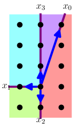
$\vbox{\hbox{\Huge$\downarrow$}}\;\varphi$

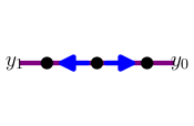
Figure 1: Toric fibration of the Hirzebruch surface $F_{3}$ over ${\mathop{\hbox{}{\mathbb{P}}}\nolimits}^{1}$.

In terms of homogeneous coordinates, the base ${\mathop{\hbox{}{\mathbb{P}}}\nolimits}^{1}$ has the usual homogeneous coordinates $[y_{0}:y_{1}]\in{\mathop{\hbox{}{\mathbb{P}}}\nolimits}^{1}$. The Hirzebruch surface is given by

$$F_{3}=\big{\{}[x_{0}:x_{1}:x_{2}:x_{3}]~{}\big{|}~{}(x_{0},x_{1})\not=(0,0),~{}(x_{2},x_{3})\not=(0,0)\big{\}}$$ (4)

subject to the homogeneous rescalings corresponding to the linear relations between the generators. Let $\vec{x}_{i}$ be the primitive lattice vector generating the ray corresponding to the homogeneous coordinate $x_{i}$, then a basis for the linear relations is

$$\vec{x}_{0}+\vec{x}_{1}+3\vec{x}_{2}=0,\quad\vec{x}_{2}+\vec{x}_{3}=0.$$ (5)

The corresponding homogeneous rescalings are

$$[x_{0}:x_{1}:x_{2}:x_{3}]=[\mu x_{0}:\mu x_{1}:\mu^{3}x_{2}:x_{3}]=[x_{0}:x_{1}:\nu x_{2}:\nu x_{3}]\quad\forall\mu,\nu\in{\mathbb{C}}^{\times}.$$ (6)

To express the toric morphism $\varphi$ in terms of the homogeneous coordinates, one needs to write the images of ray generators as non-negative linear combinations of the base ray generators. In Figure 1, this is

$$\varphi(\vec{x}_{i})=\sum_{j}\varphi_{ij}\vec{y}_{j},\quad(\varphi_{ij})=\left(\begin{smallmatrix}1&0\\ 0&1\\ 0&0\\ 0&0\end{smallmatrix}\right)a$$ (7)

and the corresponding map of homogeneous coordinates is

$$\varphi:F_{3}\to{\mathbb{C}}^{2}/\mathbb{Z}_{2}:\quad[x_{0}:x_{1}:x_{2}:x_{3}]\mapsto\left[\prod_{i}x_{i}^{\varphi_{i0}}:\prod_{i}x_{i}^{\varphi_{i1}}\right]=[x_{0}:x_{1}]$$ (8)

A point of the maximal torus orbit is characterized by all homogeneous coordinates being non-zero. Moving fibers around by the torus-action if necessary, we can the take all homogeneous coordinates to be unity. Hence, a generic toric fiber is

$$\varphi^{-1}([1:1])=\big{\{}[1:1:x_{2}:x_{3}]~{}\big{|}~{}x_{2},x_{3}\in{\mathbb{C}},~{}(x_{2},x_{3})\not=(0,0)\big{\}}={\mathop{\hbox{}{\mathbb{P}}}\nolimits}^{1}$$ (9)

Combinatorially, the generic fiber is given by the kernel fan of the toric morphism $\varphi$, that is, by the set of all cones that map to zero. In this example, the kernel fan consists of the two one-cones corresponding to $x_{2}$, $x_{3}$, and the trivial cone. There are two non-generic fiber, namely the fibers over $[y_{0}:y_{1}]=[1:0]$ and $[0:1]$. They are

$$\begin{split}\varphi^{-1}([1:0])&=\big{\{}[1:0:x_{2}:x_{3}]~{}\big{|}~{}x_{2},x_{3}\in{\mathbb{C}},~{}(x_{2},x_{3})\not=(0,0)\big{\}}={\mathop{\hbox{}{\mathbb{P}}}\nolimits}^{1},\\ \varphi^{-1}([0:1])&=\big{\{}[0:1:x_{2}:x_{3}]~{}\big{|}~{}x_{2},x_{3}\in{\mathbb{C}},~{}(x_{2},x_{3})\not=(0,0)\big{\}}={\mathop{\hbox{}{\mathbb{P}}}\nolimits}^{1}.\end{split}$$ (10)

Their embedding in $F_{3}$ is not a toric morphism, because the image is not contained in the maximal torus of $F_{3}$. Due to the simplicity of the example, the fibers over lower-dimensional torus orbits happen to be again irreducible and, in fact, isomorphic to the generic fiber. This means that the Hirzebruch surface is not only a ${\mathop{\hbox{}{\mathbb{P}}}\nolimits}^{1}$-fibration over ${\mathop{\hbox{}{\mathbb{P}}}\nolimits}^{1}$, but, in fact, a ${\mathop{\hbox{}{\mathbb{P}}}\nolimits}^{1}$-bundle.

Another well-known example of a toric morphism is the blow-up of Figure 2, which is the surjection $\mathscr{O}_{{\mathop{\hbox{}{\mathbb{P}}}\nolimits}^{1}}(-2)\to{\mathbb{C}}^{2}/\mathbb{Z}_{2}$. The corresponding fan morphism is depicted in Figure 2.

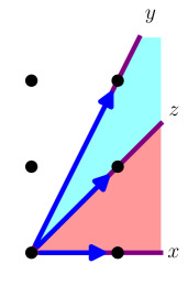
$\stackrel{{\scriptstyle\hbox{\Huge$\rightarrow$}}}{{\varphi}}$          

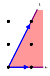
Figure 2: Blowup of ${\mathbb{C}}^{2}/\mathbb{Z}_{2}$.

Expressing the image ray generators by the ray generators of the image, one finds

$$\varphi\left(\begin{matrix}\vec{x}\\ \vec{y}\\ \vec{z}\end{matrix}\right)=\left(\begin{matrix}1&0\\ \tfrac{1}{2}&\tfrac{1}{2}\\ 0&1\\ \end{matrix}\right)\left(\begin{matrix}\vec{u}\\ \vec{v}\end{matrix}\right).$$ (11)

Hence, the map can be written in terms of homogeneous coordinates as

$$\mathscr{O}_{{\mathop{\hbox{}{\mathbb{P}}}\nolimits}^{1}}(-2)\to{\mathbb{C}}^{2}/\mathbb{Z}_{2}:\quad[x:y:z]~{}\mapsto~{}\left[x\sqrt{z}:y\sqrt{z}\right]=[u:v].$$ (12)

Note that the map apparently involves a choice of square root, however both signs lead to the same map since $[u:v]=[-u:-v]$ in ${\mathbb{C}}^{2}/\mathbb{Z}_{2}$.

There are $4$ torus orbits in $\operatorname{img}(\varphi)={\mathbb{C}}^{2}/\mathbb{Z}_{2}$, corresponding to the $4$ cones of the fan. The generic fiber is

$$\varphi^{-1}([1:1])=\big{\{}[1:1:1]\big{\}},$$ (13)

the fibers over the two one-dimensional torus orbits $v=0$ and $u=0$ are

$$\varphi^{-1}([1:0])=\big{\{}[1:1:0]\big{\}},\quad\varphi^{-1}([0:1])=\big{\{}[0:1:1]\big{\}},$$ (14)

and the fiber over the torus fixed point $u=v=0$ is

$$\varphi^{-1}([0:0])=\big{\{}[x:0:y]~{}\big{|}~{}x,y\in{\mathbb{C}},~{}(x,y)\not=(0,0)\big{\}}={\mathop{\hbox{}{\mathbb{P}}}\nolimits}^{1}$$ (15)

2.3 Fibrations of Polytopes

A particularly useful class of toric varieties are the Gorenstein Fano toric varieties. This means that they are both not too wildly singular and have enough sections of the anticanonical bundle, such that a anticanonical hypersurface is smooth after resolving the ambient space singularities. They are the face fans of reflexive lattice polytopes, or subdivisions of the face fan such that all additional rays are generated by integral points of the polytope. The duality of reflexive polytopes is mirror symmetry for the Calabi-Yau hypersurfaces.

Because the embedding of the generic fiber in the total space of a toric fibration is again a toric morphism, the fibration can already be seen on the level of the lattice polytope. Namely, the preimage of the origin in the base fan is a lattice plane in the total space polytope that intersects the reflexive polytope in a lattice sub-polytope containing the origin as a relative interior point. Note that there are only finitely many lattice sub-polytopes since each vertex must be one of the finitely many integral points of the total space polytope. Hence, it is a finite combinatorial problem to enumerate all lattice sub-polytopes in a lattice polytope. The embedding of the lattice sub-polytope is the part of the toric data that is visible just on the level of polytopes, without specifying the details of the triangulation. In the following, we refer to this as a fibration of polytopes. However, note that there is no notion of a base of the fibration when talking about polytopes alone. Indeed, as we saw in the toric morphism Figure 2, the rays of the domain fan need to map to rays of the codomain fan. In particular, this means that the integral points of the total space polytope need not map to integral points of any base polytope.

Note that it is important to identify fibrations that only differ by a lattice automorphism in order to not overcount the number of fibrations. For example, take the 24-cell, which is the reflexive 4-dimensional polytope with the largest symmetry group [17, 18]. Naively, the 24-cell lattice polytope has 34 fibrations with two-dimensional fibers. They divide into 18 fibrations whose fiber is a lattice square (the lattice polygon defining ${\mathop{\hbox{}{\mathbb{P}}}\nolimits}^{1}\times{\mathop{\hbox{}{\mathbb{P}}}\nolimits}^{1}$) and 16 fibrations whose fiber is a lattice hexagon (defining $dP_{6}$, the del Pezzo surface obtained by blowing up ${\mathop{\hbox{}{\mathbb{P}}}\nolimits}^{2}$ at 3 points). However, note the lattice symmetry group of the 24-cell is the Weyl group of $F_{4}$, which has order $1152$. By definition, the automorphism group fixes the 24-cell, but generally maps sub-polytopes to other sub-polytopes. Identifying the orbits of the fibrations, one finds that there are indeed only two different fibrations: One whose fiber is a square, and one whose fiber is a hexagon. In the following, we will always count the number of fibrations modulo automorphisms.

The naive algorithm to enumerate all $d$-dimensional fibers is to iterate over all linearly independent $d$-tuples of lattice points of the total space. They define a lattice $d$-plane. Now compute the intersection of the $d$-plane with the ambient polytope; If all vertices are integral then it defines a fibration. An important optimization over the naive algorithm is to note that one can take the $d$ vertices of the fiber to lie all on the same facet of the fiber. Hence, it suffices to iterate over $d$-tuples that simultaneously saturate one of the ambient inequalities.

It is computationally feasible to enumerate all fibrations of the $\sepnum{{.}}{{,}}{}{473800776}$ reflexive 4-dimensional polytopes. There are approximately an order of magnitude more fibrations than polytopes, though we cannot offer a precise number since we have not modded out the automorphisms for all of them. PALP [19] has an option to enumerate fibrations, but since the author does not understand some of the output the algorithm was implemented in Sage [20, 21]. See Section 3 for additional restrictions that were placed on the fibrations for the purposes of this paper, and for the results of the search.

2.4 Torus Fibrations

By a torus fibration we will always denote a fibration whose generic fiber is a real torus $T^{2}={\mathbb{C}}/(\mathbb{Z}+\tau\mathbb{Z})$. Since $T^{2}$ is not a toric variety, this cannot be realized by the fibers of a toric morphism. This is completely analogous to the fact that a toric variety itself is never a Calabi-Yau manifold, which is why one has to study hypersurfaces or complete intersections in toric varieties (which can be Calabi-Yau manifolds).

Therefore, in the following we will consider the situation where

• $\pi:X_{\Sigma}\to B$ is a toric morphism with, generically, complex 2-dimensional fibers $\pi^{-1}(b)$, $b\in B$.

• $Y\subset X_{\Sigma}$ is a Calabi-Yau fourfold hypersurface or, more generally, complete intersection.

• $Y\cap\pi^{-1}(b)\simeq T^{2}$ is a real torus (with an induced complex structure, of course) for a generic point $b\in B$.

3 Flat Fibrations

3.1 Kodaira vs. Miranda

Kodaira [22, 23] determined the structure of elliptically fibered surfaces by classifying the potential degenerate fibers in codimension one, which follow an ADE-pattern. If one wants to investigate compactifications of F-theory to six dimensions, that is, on an elliptically fibered threefold, then the degenerate fibers sit over the discriminant curve in the base. At a generic point of the curve, one can simply pick a transverse direction and reduce the local structure back to Kodaira’s case. But the curve is almost always singular, so there are codimension-two loci in the base where Kodaira’s classification is not applicable. In fact, there is no classification of codimension-two degenerate fibers in general. However, under special circumstances there is. In particular, there is a classification of codimension-two degenerate fibers [8] under the provision that the elliptic fibration is flat, that the discriminant has only normal crossings, and that the $j$-invariant of the elliptic fibration is well-defined. Even with all these restrictions, there is an infinite family of non-Kodaira degenerate fibers.

So far, I only mentioned the local structure of elliptic fibrations. The Miranda models of the degenerate fibers tell us, starting from the (singular) Weierstrass model, how the degenerate fibers in the resolved manifold look like. We are, of course, interested in compact threefolds. In order to classify the elliptically-fibered Calabi-Yau threefolds, one would then first have to classify all Weierstrass models with allowable singularities in the discriminant such that the Weierstrass model can be resolved into a smooth elliptically-fibered Calabi-Yau threefold, similar to was done in [28] for $SU(n)$ gauge groups.

For the purposes of this paper, I will be going the opposite route and start with smooth elliptically fibered Calabi-Yau threefolds. By far the largest class of such manifolds are the toric hypersurfaces [17], and I will focus on them in the following.

3.2 Toric Fibrations and Polytopes

Restricting oneself to flat fibrations, that is, fibrations whose fiber dimension is constant, is very natural if one wants to investigate fibrations over a particular base. Otherwise, one could always compose the fibration $X\to B$ with a blow-down $\pi:B\to\hat{B}$ to get a fibration $X\to\hat{B}$. So, in particular, any fibration over a blow-up of ${\mathop{\hbox{}{\mathbb{P}}}\nolimits}^{2}$ gives rise to a fibration over ${\mathop{\hbox{}{\mathbb{P}}}\nolimits}^{2}$. However, if $X\to B$ was flat then the induced fibration $X\to\hat{B}$ is most certainly not: The dimension of the fiber over the blown-up point $\hat{b}\in\hat{B}$ jumps from $\dim(X)-\dim(B)$ to $\dim(X)-\dim(B)+\dim(\pi^{-1}(\hat{B}))$. In other words, to study fibrations over a particular base (here: ${\mathop{\hbox{}{\mathbb{P}}}\nolimits}^{2}$), one should divide up the fibrations into fibrations that are flat on ${\mathop{\hbox{}{\mathbb{P}}}\nolimits}^{2}$, ${\mathop{\hbox{}{\mathbb{P}}}\nolimits}^{2}$ blown up at one point, ${\mathop{\hbox{}{\mathbb{P}}}\nolimits}^{2}$ blown up at two points, $\dots$. For the purposes of this paper, I will restrict therefore to flat fibrations over ${\mathop{\hbox{}{\mathbb{P}}}\nolimits}^{2}$, and leave the more complicated cases for future work.

In terms of toric geometry, we have already encountered the blowup $\mathscr{O}_{{\mathop{\hbox{}{\mathbb{P}}}\nolimits}^{1}}(-2)\to{\mathbb{C}}^{2}/\mathbb{Z}_{2}$ an example of a non-flat fibration, see Figure 2. The reason for why the fiber dimension is not constant in this example is that one of the rays of the domain fan maps to a higher-dimensional cone (in this case, the $2$-cone $\left<u,v\right>$) of the codomain fan. This means that there is a point in the base (the torus orbit corresponding to the $2$-cone) whose fiber is given by the vanishing of a single homogeneous coordinate, see eq. (15). Clearly, this cannot be a flat fibration. A necessary criterion for a flat fibration is that the rays of the domain fan map either to zero or the rays of the codomain fan, but not into any higher-dimensional cone. A necessary and sufficient criterion [15] is that every primitive cone of the domain fan (not just the one-dimensional ones) maps bijectively to its image cone.

Therefore, for flat fibrations we can read of the base rays from the polytope alone, without having to triangulate the total space polytope: The rays of the base fan must be the images of the rays of the total space fan.

3.3 Classification of Fibered Polytopes

As we saw above, for a flat fibration the rays of the base fan are determined by the rays of the total space fan. For the purposes of this paper, we will be interested in the Gorenstein Fano $4$-dimensional toric varieties fibered over ${\mathop{\hbox{}{\mathbb{P}}}\nolimits}^{2}$. As with all toric surfaces, the whole fan of ${\mathop{\hbox{}{\mathbb{P}}}\nolimits}^{2}$ is determined by the rays. Furthermore, we want to have a smooth Calabi-Yau hypersurface. For this, we need to subdivide the face fan of the reflexive 4-dimensional polytope such that all integral points that are not interior to facets span a ray.

To summarize, on the level of polytopes we can enumerate the flat fibrations over ${\mathop{\hbox{}{\mathbb{P}}}\nolimits}^{2}$ by the following steps. For all reflexive 4-dimensional polytopes $P$:

• Find all lattice sub-polytopes $S\subset P$

• Project all integral points not interior to a facet of $P$.

• Test whether the projected points span the rays of the fan of ${\mathop{\hbox{}{\mathbb{P}}}\nolimits}^{2}$.

• Identify fibrations that map to each other by the action of $\operatorname{Aut}_{\mathbb{Z}}(P)=\operatorname{Aut}(P)\cap GL(4,\mathbb{Z})$.

Searching this way through the list of $\sepnum{{.}}{{,}}{}{473800776}$ reflexive 4-dimensional polytopes, we find $\sepnum{{.}}{{,}}{}{102581}$ distinct fibered polytopes corresponding to flat fibrations over ${\mathop{\hbox{}{\mathbb{P}}}\nolimits}^{2}$.

The largest number of distinct fibered polytopes ($774$) is found for the Hodge numbers $h^{11}=14$, $h^{21}=26$. The distribution of Hodge numbers is shown in Figures 3 and 4.

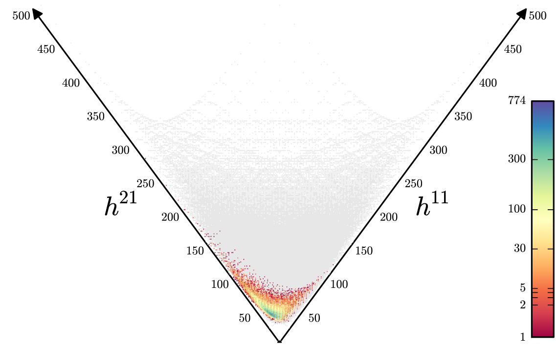
Figure 3: The distribution of flat toric elliptic fibrations with base ${\mathop{\hbox{}{\mathbb{P}}}\nolimits}^{2}$.

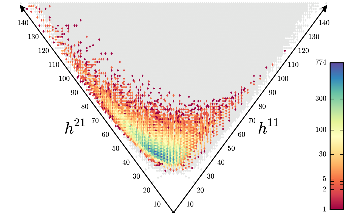
Figure 4: The region of heights $h^{11}+h^{21}\leq 150$ in Figure 3.

3.4 Weierstrass Models

Before passing to explicit examples where the complete geometry will be specified, there is one more piece of information that does not depend on the details of how the fibration of polytopes is resolved into a fibration of toric varieties. This is the Weierstrass model of the elliptic fibration, obtained by bringing the hypersurface equation into Weierstrass form $y^{2}=x^{3}+ax+b$ over the maximal torus of the base. Obtaining the correct Weierstrass form depends on having enough rays in the fan of the toric variety, but is otherwise independent of the details of the details of the fan.

In terms of homogeneous coordinates, it is convenient to use projective coordinates $[u:v:w]\in{\mathop{\hbox{}{\mathbb{P}}}\nolimits}^{2}$ for the base ${\mathop{\hbox{}{\mathbb{P}}}\nolimits}^{2}$ and affine coordinates $(x,y)$ on the fiber. Then pick a parametrization of the maximal torus of the total space fan such that

• $\vec{u}$, $\vec{v}$, and $\vec{w}$ map to the three generators of the base ${\mathop{\hbox{}{\mathbb{P}}}\nolimits}^{2}$-fan.

• If the fiber fan is the fan of ${\mathop{\hbox{}{\mathbb{P}}}\nolimits}^{2}$, the $2$-cone $\left<x,y\right>$ can be any $2$-cone.

• If the fiber fan is a blow-up of ${\mathop{\hbox{}{\mathbb{P}}}\nolimits}^{2}$, pick $\left<x\right>$ and $\left<y\right>$ to be cones that survive after blowing down to ${\mathop{\hbox{}{\mathbb{P}}}\nolimits}^{2}$.

• Otherwise, for example if the fiber fan is ${\mathop{\hbox{}{\mathbb{P}}}\nolimits}^{1}\times{\mathop{\hbox{}{\mathbb{P}}}\nolimits}^{1}$, pick suitable coordinates to bring the (not necessarily cubic) equation into Weierstrass form, see Appendix A for how this can be done for any fiber reflexive polygon.

Having chosen $3+2$ rays in this manner, we just need to set all other homogeneous coordinates equal to one in the hypersurface equation. The result is a cubic in $x$, $y$ that can easily be brought into Weierstrass form. In the remainder of this paper, we will now look at three increasingly more complicated examples of how toric elliptic fibrations can be analyzed.

4 An Example of a Toric Elliptic Fibration

4.1 Fibration of the Polytope

As the first example, consider the reflexive polytope with vertices

$$P=\operatorname{conv}\left\{\left(\begin{smallmatrix}-3\\ 0\\ -1\\ -1\end{smallmatrix}\right),\left(\begin{smallmatrix}-1\\ 2\\ -1\\ -1\end{smallmatrix}\right),\left(\begin{smallmatrix}0\\ -1\\ 0\\ 0\end{smallmatrix}\right),\left(\begin{smallmatrix}0\\ 0\\ 0\\ 1\end{smallmatrix}\right),\left(\begin{smallmatrix}0\\ 0\\ 1\\ 0\end{smallmatrix}\right),\left(\begin{smallmatrix}0\\ 1\\ 0\\ 0\end{smallmatrix}\right),\left(\begin{smallmatrix}0\\ 2\\ -1\\ -1\end{smallmatrix}\right),\left(\begin{smallmatrix}1\\ 0\\ 0\\ 0\end{smallmatrix}\right),\left(\begin{smallmatrix}2\\ 0\\ -1\\ -1\end{smallmatrix}\right)\right\}.$$ (16)

In addition to the vertices and the origin, the lattice polytope $P$ has 9 further integral points

$$P\owns\left(\begin{smallmatrix}-2\\ 0\\ -1\\ -1\end{smallmatrix}\right),\left(\begin{smallmatrix}-2\\ 1\\ -1\\ -1\end{smallmatrix}\right),\left(\begin{smallmatrix}-1\\ 0\\ -1\\ -1\end{smallmatrix}\right),\left(\begin{smallmatrix}-1\\ 0\\ 0\\ 0\end{smallmatrix}\right),\left(\begin{smallmatrix}-1\\ 1\\ -1\\ -1\end{smallmatrix}\right),\left(\begin{smallmatrix}0\\ 0\\ -1\\ -1\end{smallmatrix}\right),\left(\begin{smallmatrix}0\\ 1\\ -1\\ -1\end{smallmatrix}\right),\left(\begin{smallmatrix}1\\ 0\\ -1\\ -1\end{smallmatrix}\right),\left(\begin{smallmatrix}1\\ 1\\ -1\\ -1\end{smallmatrix}\right),$$ (17)

none of which are interior to a facet of $P$. Moreover, $P$ is a lattice polytope fibration with respect to the sub-polytope

$$P\cap\big{(}\mathbb{Z}\oplus\mathbb{Z}\oplus\{0\}\oplus\{0\}\big{)}=\operatorname{conv}\left\{\left(\begin{smallmatrix}-1\\ 0\\ 0\\ 0\end{smallmatrix}\right),\left(\begin{smallmatrix}0\\ -1\\ 0\\ 0\end{smallmatrix}\right),\left(\begin{smallmatrix}0\\ 1\\ 0\\ 0\end{smallmatrix}\right),\left(\begin{smallmatrix}1\\ 0\\ 0\\ 0\end{smallmatrix}\right)\right\}.$$ (18)

which we recognize as the lattice polygon of ${\mathop{\hbox{}{\mathbb{P}}}\nolimits}^{1}\times{\mathop{\hbox{}{\mathbb{P}}}\nolimits}^{1}$. The lattice projection onto the base is, clearly,

$$\varphi=\begin{pmatrix}0&0&1&0\\ 0&0&0&1\\ \end{pmatrix},$$ (19)

and all integral points of $P$ not interior to facets map to the standard rays of the fan of ${\mathop{\hbox{}{\mathbb{P}}}\nolimits}^{2}$, whose rays we label $\left<u\right>$, $\left<v\right>$, and $\left<w\right>$ as in Figure 5.

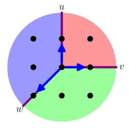
Figure 5: The fan of ${\mathop{\hbox{}{\mathbb{P}}}\nolimits}^{2}$.

What makes $P$ a particularly simple example is that there is exactly one point over the two base rays $\left<u\right>$ and $\left<v\right>$. Hence, the fibers over the corresponding torus orbits $\{u=0,wv\not=0\}$ and $\{v=0,uw\not=0\}$ in the base ${\mathop{\hbox{}{\mathbb{P}}}\nolimits}^{2}$ are the same as the generic fiber. Only over the toric divisor $\{w=0\}\subset{\mathop{\hbox{}{\mathbb{P}}}\nolimits}^{2}$ do we get a more interesting fiber. More specific, there are $19$ integral points in $P$:

• one point is over $\vec{u}$ and $\vec{v}$ each,

• the fiber polytope $\varphi^{-1}(0)$ consists of 5 points, the origin and the four vertices of the ${\mathop{\hbox{}{\mathbb{P}}}\nolimits}^{1}\times{\mathop{\hbox{}{\mathbb{P}}}\nolimits}^{1}$ lattice square,

• the remaining $12$ integral points are contained in the $2$-face $F=P\cap\varphi^{-1}(\vec{w})$, see Figure 6.

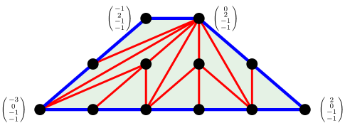
Figure 6: The two-face $F\subset P$ and its triangulation used in Subsection 4.4.

and much of the information about the triangulation of $P$, that is, the subdivision of the face fan of $P$, is contained in the triangulation of this two-face $F$.

The simplest toric variety one can construct from $P$ is its face fan (14 generating cones), but this toric variety is not fibered. The problem is that $\varphi$ projects some $2$-faces of $P$ to $\operatorname{conv}\{\vec{u},\vec{v},\vec{w}\}$, so the corresponding cone of the face fan is not contained in any single cone of the base. However, there is a well-defined procedure to subdivide the face fan along the half-planes $\varphi^{-1}(\left<u\right>)$, $\varphi^{-1}(\left<v\right>)$, and $\varphi^{-1}(\left<w\right>)$ that will lead to the minimal fibered toric variety, that is, the coarsest partial resolution of the face fan such that the toric variety is fibered (18 generating cones in this example).

4.2 Weierstrass Model

The minimal fibered toric variety and any contained anticanonical hypersurface is still very singular, but it is good enough to determine the Weierstrass model. Following Appendix A, let us parametrize the maximal torus by picking five homogeneous coordinates

$$\vec{u}=\left(\begin{smallmatrix}0\\ 0\\ 0\\ 1\end{smallmatrix}\right),\quad\vec{v}=\left(\begin{smallmatrix}0\\ 0\\ 1\\ 0\end{smallmatrix}\right),\quad\vec{w}=\left(\begin{smallmatrix}-1\\ 2\\ -1\\ -1\end{smallmatrix}\right),\quad\vec{x}=\left(\begin{smallmatrix}1\\ 0\\ 0\\ 0\end{smallmatrix}\right),\quad\vec{y}=\left(\begin{smallmatrix}0\\ 1\\ 0\\ 0\end{smallmatrix}\right).$$ (20)

The dual polytope $P^{*}$ has $35$ integral points, hence the equation of a Calabi-Yau hypersurface has $35$ distinct monomials in the homogeneous coordinates. Setting all other homogeneous variables to unity, the

$$\begin{gathered}\{uw^{5}y^{2},\ vw^{5}y^{2},\ w^{6}y^{2},\ u^{3}w^{2}xy^{2},\ u^{2}vw^{2}xy^{2},\ uv^{2}w^{2}xy^{2},\ v^{3}w^{2}xy^{2},\ u^{2}w^{3}xy^{2},\ \\ uvw^{3}xy^{2},\ v^{2}w^{3}xy^{2},\ uw^{4}xy^{2},\ vw^{4}xy^{2},\ w^{5}xy^{2},\ w^{4}x^{2}y^{2},\ uw^{3}y,\ vw^{3}y,\ \\ w^{4}y,\ u^{3}xy,\ u^{2}vxy,\ uv^{2}xy,\ v^{3}xy,\ u^{2}wxy,\ uvwxy,\ v^{2}wxy,\ uw^{2}xy,\ \\ vw^{2}xy,\ w^{3}xy,\ w^{2}x^{2}y,\ uw,\ vw,\ w^{2},\ ux,\ vx,\ wx,\ x^{2}\}\end{gathered}$$ (21)

A generic linear combination is not a cubic in the fiber coordinates $x$, $y$ because of the $w^{4}x^{2}y^{2}$ term. This comes as no surprise, since an anticanonical hypersurface in the ${\mathop{\hbox{}{\mathbb{P}}}\nolimits}^{1}\times{\mathop{\hbox{}{\mathbb{P}}}\nolimits}^{1}$ fiber is a biquadric in $x$ and $y$. Of course a smooth biquadric in ${\mathop{\hbox{}{\mathbb{P}}}\nolimits}^{1}\times{\mathop{\hbox{}{\mathbb{P}}}\nolimits}^{1}$ is isomorphic to some cubic in ${\mathop{\hbox{}{\mathbb{P}}}\nolimits}^{2}$, so there is a way to bring it into Weierstrass form. This works as follows [29]. Given a biquadric

$$q(x,y)=\alpha_{22}x^{2}y^{2}+\alpha_{21}x^{2}y+\alpha_{20}x^{2}+\alpha_{12}xy^{2}+\alpha_{11}xy+x\alpha_{10}+y^{2}\alpha_{02}+y\alpha_{01}+\alpha_{00},$$ (22)

first compute the usual quadratic discriminant with respect to $y$,

$$\beta_{4}x^{4}+\beta_{3}x^{3}+\beta_{2}x^{2}+\beta_{1}x+\beta_{0}=\left(\sum\alpha_{i1}x^{i}\right)^{2}-4\left(\sum\alpha_{i2}x^{i}\right)\left(\sum\alpha_{i0}x^{i}\right).$$ (23)

The coefficients $a$, $b$ of the Weierstrass form $y^{2}=x^{3}+ax+b$ are then given by the quadratic and cubic projective $GL(2,{\mathbb{C}})$-invariants of the resulting plane quartic,

$$\begin{split}a=&-\tfrac{1}{4}\big{(}\beta_{0}\beta_{4}+3\beta_{2}^{2}-4\beta_{1}\beta_{3}\big{)}\\ b=&-\tfrac{1}{4}\big{(}\beta_{0}\beta_{3}^{2}+\beta_{1}^{2}\beta_{4}-\beta_{0}\beta_{2}\beta_{4}-2\beta_{1}\beta_{2}\beta_{3}+\beta_{2}^{3}\big{)}.\end{split}$$ (24)

4.3 Gauge Group

It is now an easy exercise to bring any chosen Calabi-Yau hypersurface into Weierstrass form with $35$ free parameters. However, due to the number of coefficients the result will be unwieldy. For illustration, we will therefore pick the following “random” coefficients for the monomials in eq. (21)

$$\begin{gathered}(1,2,-2,1,2,2,1,-2,0,0,2,1,-1,2,2,2,1,-1,\hskip 56.9055pt\\ \hskip 56.9055pt0,0,-1,1,1,0,2,2,2,2,-1,-2,2,2,-1,-1,1)\end{gathered}$$ (25)

Fiber	$I_{0}$	$I_{n}$	$II$	$III$	$IV$	$I_{0}^{*}$	$I_{n}^{*}$	$IV^{*}$	$III^{*}$	$II^{*}$
$\operatorname{ord}(a)$	$\geq 0$	$0$	$\geq 0$	$1$	$\geq 2$	$\geq 2$	$2$	$\geq 3$	$3$	$\geq 4$
$\operatorname{ord}(b)$	$\geq 0$	$0$	$1$	$\geq 2$	$2$	$\geq 3$	$3$	$4$	$\geq 5$	$5$
$\operatorname{ord}(\Delta)$	$0$	$n$	$2$	$3$	$4$	$6$	$n+6$	$8$	$9$	$10$

Table 1: Tate’s algorithm [1] for the Kodaira fiber of a Weierstrass equation.

We have verified that these are sufficiently random in the sense that any other generic choice will lead to the same orders of vanishing and factorizations in the following. The coefficients and discriminant of the Weierstrass form are, then,

$$\begin{split}a&=-\tfrac{1}{48}\big{(}16u^{12}-32u^{10}v^{2}+32u^{9}v^{3}+\cdots-71w^{12}\big{)}\\ b&=\tfrac{1}{864}\big{(}64u^{18}-192u^{16}v^{2}+192u^{15}v^{3}+\cdots+269w^{18}\big{)}\\ \Delta&=-\tfrac{1}{16}\;w^{10}\;\big{(}1024u^{26}+2048u^{25}v-11008u^{24}v^{2}+\cdots-249w^{26}\big{)}\end{split}$$ (26)

where the factors containing the ellipses are irreducible (and contain a great number of terms). Using Table 1, we can immediately read off that the discriminant divisor splits into an $I_{10}$ component along the toric divisor ${w=0}\subset{\mathop{\hbox{}{\mathbb{P}}}\nolimits}^{2}$ and an $I_{1}$ component on a degree-$26$ curve.

The low-energy gauge group depends on the Kodaira type along each discriminant component as well as the monodromy of the Kodaira fiber. Whether or not there is a monodromy can also be read off from the Weierstrass model [1, 30, 7, 31]. For the $I_{m}$ case, $m\geq 3$, this depends on whether $\tfrac{b}{a}$ restricted to the discriminant is a square or not. In the case at hand one obtains

$$\left.\frac{b}{a}\right|_{w=0}=-\tfrac{1}{18}(u+v)^{2}\big{(}2u^{2}-2uv+v^{2}\big{)}^{2}.$$ (27)

Hence we are in the “split” case, and the gauge group is $SU(10)$. As we will see in the next subsection, the fact that there is no monodromy can be nicely be seen from the toric geometry of the resolved Calabi-Yau threefold.

4.4 Resolution of Singularities

So far, we only discussed the Weierstrass model without going into the details of the resolution of singularities. Really, this is the essential novelty of the approach taken in this paper: By starting from the maximal resolutions of Gorenstein Fano toric varieties, we have complete control over the desingularization of the Weierstrass model. In particular, the details of the resolution of singularities are visible and the Hodge numbers can be readily computed.

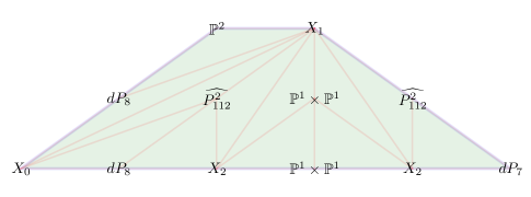
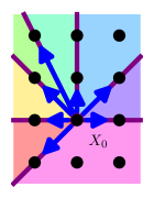
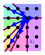
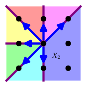
Figure 7: The irreducible fiber components over $w=0$. The top row shows the different toric surfaces that form the irreducible components. The bottom row consists of the fans defining the surfaces $X_{0}$, $X_{1}$, and $X_{2}$ that do not have standard names.

To crepantly desingularize the toric variety, we need to subdivide the fan into smooth (that is, simplicial and unimodular) cones using the rays through all of the integral points of the polytope. In particular, one has to utilize the remaining $8$ integral points in the triangulation of $P$. Any such smooth triangulation has 56 generating cones. To be completely explicit, we will be using a particular triangulation that is uniquely determined by admitting a toric fibration together with the induced triangulation of the two-face $F\subset P$ shown in Figure 6. Using this fan, there are $12$ primitive [15] preimage cones over $\left<w\right>$, namely the $12$ integral points of the two-face $F$. Therefore, the toric fiber over $w=0$ in the total space consists of $12$ irreducible components. Each irreducible component is a toric surface, and they are joined along common ${\mathop{\hbox{}{\mathbb{P}}}\nolimits}^{1}$ as the corresponding points of the induced triangulation of $F$. The details of all toric fiber components are shown in Figure 7.

The Calabi-Yau hypersurface can, but does not have to, intersect the toric fiber components. To determine the Kodaira type of the degenerate elliptic fiber, one needs to restrict the anticanonical divisor on the ambient toric variety to each of the irreducible components of the toric fiber. One finds that the restriction is trivial for the two toric fiber components in the interior of the two-face $F$, and nontrivial for the $10$ toric fiber components corresponding to the points on the boundary of $F$. This is how the Kodaira fiber $I_{10}$ arises over the $w=0$ component of the discriminant in the elliptic fibration:

• The Calabi-Yau hypersurface intersects each of the $10$ two-dimensional toric fibers on the boundary of $F$ in a ${\mathop{\hbox{}{\mathbb{P}}}\nolimits}^{1}$.

• There is a one-dimensional fiber component (where two $2$-dimensional components intersect) for each of the lines of the triangulation of $F$. The Calabi-Yau hypersurface intersects each of the $10$ blue lines in Figure 7 in a point, and does not intersect any of the $13$ red lines.

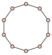
Figure 8: The fiber-divisor-graph $F(\langle w\rangle,-K)$ for the fiber over the discriminant component $w=0$. It is the $\tilde{A}_{9}$ extended Dynkin diagram corresponding to an $I_{10}$ Kodaira fiber.

Hence, in this example the graph of the $I_{10}$ Kodaira fiber (that is, the $\tilde{A}_{9}$ extended Dynkin diagram) is visible as the graph of integral points on $\partial F$ and their connecting edges [32, 33, 34, 35, 36, 37]. As we will see in the next section, this is not always true. However, much of the information about the Kodaira fiber can be derived from the pull-back of the anticanonical divisor to the toric fibers. A nice graphical representation of this data is what we will call the fiber divisor graph in the following:

Definition 1 (Fiber-Divisor-Graph).

Let $\pi:X\to B$ be a toric fibration with $2$-dimensional fibers and $\dim(X)=4$. For a fixed toric fiber $\pi^{-1}(p)=\cup F_{i}$ and nef divisor $D\subset X$, let $F(p,D)$ be the graph with

• one node for each fiber irreducible component $F_{i}$ such that $[D|_{F_{i}}]\not=0$, and

• $\mathbb{Z}_{\geq 0}\owns D\cap F_{i}\cap F_{j}$ edges joining $F_{i}$ and $F_{j}$.

The fiber-divisor-graph only depends on the torus orbit of the base point $p\in B$ (that is, a cone of the fan of $B$) and the divisor class $[D]$.

For example, the fiber-divisor-graph $F(\langle w\rangle,-K)$ for the example discussed in this section is shown in Figure 8.

5 Non-Split Fibrations

5.1 Weierstrass Model

We now turn to a more complicated example that will explain how to deal with various issues in classifying the gauge groups of toric elliptic fibrations. Apart from the origin, the polytope contains the integral points in the following table:

$$\begin{array}[]{|cccccc|ccccccccc|cc|}\hline\cr s_{0}&s_{1}&s_{2}&s_{3}&s_{4}&s_{5}&s_{6}&s_{7}&\lx@intercol\hfil\hfil\lx@intercol\vrule\lx@intercol\\ \hline\cr t_{0}&t_{1}&t_{2}&t_{3}&t_{4}&t_{5}&t_{6}&t_{7}&t_{8}&t_{9}&t_{10}&t_{11}&t_{12}&t_{13}&t_{14}&t_{15}&t_{16}\\ \hline\cr-2&-2&0&0&1&0&0&0&-2&-1&-1&-1&0&0&0&-1&0\\ -2&-2&1&1&0&0&0&0&-2&-1&-1&-1&1&1&1&-1&0\\ -5&-5&0&0&0&1&-1&-1&-5&-3&-3&-2&0&0&0&-3&-1\\ -5&-3&0&4&0&0&-1&1&-4&-3&-1&-2&1&2&3&-2&0\\ \hline\cr\vrule\lx@intercol\hfil\text{vertices}\hfil\lx@intercol\vrule\lx@intercol&\lx@intercol\hfil\text{not interior to facets}\hfil\lx@intercol\vrule\lx@intercol&\lx@intercol\hfil\text{rest}\hfil\lx@intercol\vrule\lx@intercol\\ \hline\cr\end{array}$$ (28)

The first 6 points are the vertices, the middle 9 points are integral points that are not interior to facets, and the last 2 points are interior to facets. The eight $s_{i}$ are the homogeneous coordinates necessary to write the Weierstrass model; the seventeen $t_{j}$ are the homogeneous coordinates necessary to completely desingularize the elliptically fibered Calabi-Yau hypersurface and will only play a role in the next subsection.

The most coarse toric variety would use only the vertices as rays of the fan, but this alone is not sufficient for a toric fibration. In particular, we will use the toric morphism defined by the projection onto the first two coordinates, that is,

$$\varphi(\vec{n})=\begin{pmatrix}1&0&0&0\\ 0&1&0&0\\ \end{pmatrix}\vec{n}$$ (29)

A minimal subdivision of the face fan for which $\varphi$ does define a toric fibration is generated by the following $16$ four-dimensional cones:

$$\begin{gathered}\smash{\Big{\{}}\langle s_{0},s_{1},s_{2},s_{3},s_{6},s_{7}\rangle,\langle s_{0},s_{1},s_{4},s_{6},s_{7}\rangle,\langle s_{0},s_{1},s_{2},s_{3},s_{5}\rangle,\langle s_{0},s_{1},s_{4},s_{5}\rangle,\hfill\\ \langle s_{0},s_{2},s_{5},s_{6}\rangle,\langle s_{0},s_{4},s_{5},s_{6}\rangle,\langle s_{2},s_{3},s_{4},s_{6},s_{7}\rangle,\langle s_{1},s_{3},s_{5},s_{7}\rangle,\\ \hfill\langle s_{1},s_{4},s_{5},s_{7}\rangle,\langle s_{2},s_{4},s_{5},s_{6}\rangle,\langle s_{2},s_{3},s_{4},s_{5}\rangle,\langle s_{3},s_{4},s_{5},s_{7}\rangle\smash{\Big{\}}}\end{gathered}$$ (30)

In order to write the Weierstrass form on the maximal torus, we need to pick coordinates. A slight complication is that there is no ray whose generator maps onto the generator $\vec{w}$ of the base ${\mathop{\hbox{}{\mathbb{P}}}\nolimits}^{2}$ fan, see Figure 5. We only have $\vec{s}_{0}$ and $\vec{s}_{1}$ at our disposal, and both map to $2\vec{w}$. Hence a choice of coordinates that map to the base homogeneous coordinates necessarily involves square roots, for example

$$\autoref{eq:toricmorphismroot}[s_{0}:\cdots:s_{7}]=[\sqrt{w}:1:v:1:u:1:1:1]$$ (31)

Written in terms of $u,v,w$, the hypersurface equation will contain fractional powers of $w$, but the Weierstrass form will be polynomial. The dual polytope contains $44$ integral points, so there are $44$ monomials in the Calabi-Yau hypersurface equation. The generic fiber is the weighted projective space ${\mathop{\hbox{}{\mathbb{P}}}\nolimits}^{2}[1,1,2]$, for which we explain in Appendix A how to compute the Weierstrass form. The result is that

$$a=P_{10}(u,v,w),\qquad b=P_{15}(u,v,w),\qquad\Delta=v^{8}w^{2}P_{20}(u,v,w),$$ (32)

where $P_{d}$ is an irreducible polynomial of degree $d$. Hence, the elliptic fiber over $u=0$ is a smooth elliptic curve, the fiber over $v=0$ is an $I_{8}$ Kodaira fiber. Depending on the monodromy of this $I_{8}$ fiber, the gauge group can be $SU(8)$ or $Sp(4)$. In this case, one finds that the monodromy cover $\tfrac{b}{a}\big{|}_{v=0}$ is not a square, hence it is of non-split type.

For the fiber over $w=0$, one needs to be more careful. Clearly the discriminant vanishes to second order in $w$, but the good local ambient space coordinate is $\pm\sqrt{w}$. Hence the corresponding Kodaira fiber is not $I_{2}$ but $I_{2}^{*}$. This can also be derived by direct computation if one resolves the fan further, for example the desingularization to be discussed in the following subsection adds new rays such that some ray generator (for example, $\vec{t}_{9}$) now maps onto $\vec{w}$. So by using $t_{9}$ instead of $s_{0}$ as local coordinate on the ambient toric variety, the toric morphism can be written in terms of polynomials and one obtains the expected Weierstrass form

$$a=w^{2}P_{10}(u,v,w),\qquad b=w^{3}P_{15}(u,v,w),\qquad\Delta=v^{8}w^{8}P_{20}(u,v,w).$$ (33)

Finally, the monodromy cover $\tfrac{\Delta}{w^{8}}\big{(}\tfrac{aw}{b}\big{)}^{2}|_{w=0}=\psi^{2}$ factors into the square of a polynomial, so the $I_{2}^{*}$ component is of split type.

To summarize, the three toric divisors on the base ${\mathop{\hbox{}{\mathbb{P}}}\nolimits}^{3}$ support the following gauge groups:

• $u=0:$ Elliptic fiber is smooth (Kodaira fiber $I_{0}$), no gauge group.

• $v=0:$ Kodaira fiber of type $I_{8}$, non-split, gauge group $Sp(4)$.

• $w=0:$ Kodaira fiber of type $I_{2}^{*}$, split, gauge group $SO(12)$.

5.2 Resolution of Singularities

The Weierstrass model is just a singular model for the smooth elliptic fibration in the sense of the minimal model program. We now desingularize the ambient toric variety, which resolves the Calabi-Yau hypersurface into a smooth threefold with Hodge numbers $(h^{11},h^{21})=(19,35)$. This amounts to subdividing the fan until all cones of dimension $\leq 3$ are smooth. In the following, we will be using the resolution of the fan generated by the $56$ cones

$$\begin{gathered}\scriptstyle\langle t_{0},t_{2},t_{5},t_{9}\rangle,\langle t_{0},t_{2},t_{5},t_{12}\rangle,\langle t_{0},t_{2},t_{9},t_{15}\rangle,\langle t_{0},t_{2},t_{12},t_{15}\rangle,\langle t_{0},t_{3},t_{5},t_{11}\rangle,\langle t_{0},t_{3},t_{5},t_{14}\rangle,\langle t_{0},t_{3},t_{8},t_{11}\rangle,\langle t_{0},t_{3},t_{8},t_{15}\rangle,\\ \scriptstyle\langle t_{0},t_{3},t_{14},t_{15}\rangle,\langle t_{0},t_{4},t_{5},t_{9}\rangle,\langle t_{0},t_{4},t_{5},t_{11}\rangle,\langle t_{0},t_{4},t_{8},t_{11}\rangle,\langle t_{0},t_{4},t_{8},t_{15}\rangle,\langle t_{0},t_{4},t_{9},t_{15}\rangle,\langle t_{0},t_{5},t_{12},t_{13}\rangle,\langle t_{0},t_{5},t_{13},t_{14}\rangle,\\ \scriptstyle\langle t_{0},t_{12},t_{13},t_{15}\rangle,\langle t_{0},t_{13},t_{14},t_{15}\rangle,\langle t_{1},t_{3},t_{5},t_{10}\rangle,\langle t_{1},t_{3},t_{5},t_{11}\rangle,\langle t_{1},t_{3},t_{8},t_{10}\rangle,\langle t_{1},t_{3},t_{8},t_{11}\rangle,\langle t_{1},t_{4},t_{5},t_{10}\rangle,\langle t_{1},t_{4},t_{5},t_{11}\rangle,\\ \scriptstyle\langle t_{1},t_{4},t_{8},t_{10}\rangle,\langle t_{1},t_{4},t_{8},t_{11}\rangle,\langle t_{2},t_{4},t_{5},t_{6}\rangle,\langle t_{2},t_{4},t_{5},t_{12}\rangle,\langle t_{2},t_{4},t_{6},t_{16}\rangle,\langle t_{2},t_{4},t_{7},t_{12}\rangle,\langle t_{2},t_{4},t_{7},t_{16}\rangle,\langle t_{2},t_{5},t_{6},t_{9}\rangle,\\ \scriptstyle\langle t_{2},t_{6},t_{9},t_{16}\rangle,\langle t_{2},t_{7},t_{9},t_{15}\rangle,\langle t_{2},t_{7},t_{9},t_{16}\rangle,\langle t_{2},t_{7},t_{12},t_{15}\rangle,\langle t_{3},t_{4},t_{5},t_{7}\rangle,\langle t_{3},t_{4},t_{5},t_{14}\rangle,\langle t_{3},t_{4},t_{7},t_{14}\rangle,\langle t_{3},t_{5},t_{7},t_{10}\rangle,\\ \scriptstyle\langle t_{3},t_{7},t_{8},t_{10}\rangle,\langle t_{3},t_{7},t_{8},t_{15}\rangle,\langle t_{3},t_{7},t_{14},t_{15}\rangle,\langle t_{4},t_{5},t_{6},t_{9}\rangle,\langle t_{4},t_{5},t_{7},t_{10}\rangle,\langle t_{4},t_{5},t_{12},t_{13}\rangle,\langle t_{4},t_{5},t_{13},t_{14}\rangle,\langle t_{4},t_{6},t_{9},t_{16}\rangle,\\ \scriptstyle\langle t_{4},t_{7},t_{8},t_{10}\rangle,\langle t_{4},t_{7},t_{8},t_{15}\rangle,\langle t_{4},t_{7},t_{9},t_{15}\rangle,\langle t_{4},t_{7},t_{9},t_{16}\rangle,\langle t_{4},t_{7},t_{12},t_{13}\rangle,\langle t_{4},t_{7},t_{13},t_{14}\rangle,\langle t_{7},t_{12},t_{13},t_{15}\rangle,\langle t_{7},t_{13},t_{14},t_{15}\rangle.\end{gathered}$$ (34)

The corresponding toric variety still has point-like orbifold singularities, but they will be missed by a generic Calabi-Yau hypersurface.

It is a subtle point that we need to add the rays through the points $\vec{t}_{15}$ and $\vec{t}_{16}$ that are in the interior of a facet of the polytope to resolve the toric variety to be smooth except for point singularities and, at the same time, be fibered over ${\mathop{\hbox{}{\mathbb{P}}}\nolimits}^{2}$ by $\varphi$. If we would not require the fibration structure, we could just merge the generating cones containing $\vec{t}_{15}$, $\vec{t}_{16}$, that is, replace

$$\begin{split}\left\{\begin{smallmatrix}\langle t_{0},t_{3},t_{8},t_{15}\rangle,\langle t_{3},t_{7},t_{8},t_{15}\rangle,\langle t_{4},t_{7},t_{8},t_{15}\rangle,\langle t_{0},t_{4},t_{8},t_{15}\rangle,\\ \langle t_{4},t_{7},t_{9},t_{15}\rangle,\langle t_{0},t_{4},t_{9},t_{15}\rangle,\langle t_{2},t_{7},t_{9},t_{15}\rangle,\langle t_{0},t_{2},t_{9},t_{15}\rangle,\\ \langle t_{0},t_{2},t_{12},t_{15}\rangle,\langle t_{2},t_{7},t_{12},t_{15}\rangle,\langle t_{0},t_{12},t_{13},t_{15}\rangle,\langle t_{7},t_{12},t_{13},t_{15}\rangle,\\ \langle t_{0},t_{3},t_{14},t_{15}\rangle,\langle t_{3},t_{7},t_{14},t_{15}\rangle,\langle t_{0},t_{13},t_{14},t_{15}\rangle,\langle t_{7},t_{13},t_{14},t_{15}\rangle\end{smallmatrix}\right\}\longrightarrow&~{}\langle t_{0},t_{2},t_{3},t_{4},t_{7},t_{8},t_{9},t_{12},t_{13},t_{14}\rangle,\\ \left\{\begin{smallmatrix}\langle t_{2},t_{4},t_{6},t_{16}\rangle,\langle t_{2},t_{4},t_{7},t_{16}\rangle,\langle t_{4},t_{7},t_{9},t_{16}\rangle,\\ \langle t_{4},t_{6},t_{9},t_{16}\rangle,\langle t_{2},t_{7},t_{9},t_{16}\rangle,\langle t_{2},t_{6},t_{9},t_{16}\end{smallmatrix}\right\}\longrightarrow&~{}\langle t_{2},t_{4},t_{6},t_{7},t_{9}\rangle.\end{split}$$ (35)

The resulting toric variety would still only have point singularities, but would no longer be torically fibered.

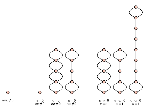
Figure 9: The fiber-divisor-graph $F(O(\sigma),-K)$ of the $I_{8}I_{2}^{*}$-fibration over the $7$ torus-orbits $O(\sigma)$, $\sigma\in\Sigma$, in the base ${\mathop{\hbox{}{\mathbb{P}}}\nolimits}^{2}={\mathop{\hbox{}{\mathbb{P}}}\nolimits}_{\Sigma}$.

Using the resolved fan eq. (34), it is now a straightforward exercise to compute the restriction of the anticanonical divisor to each toric fiber. The fiber-divisor-graph introduced in Subsection 4.4 is a useful way of visualizing the result, and can be seen in Figure 9. One immediately notices that the graphs of the fibers over $v=0$ and $w=0$ do not look like the graphs of the expected $I_{8}$ and $I_{2}^{*}$ Kodaira fibers. In fact, the fiber-divisor-graph over $v=0$ cannot be the $\tilde{A}_{7}$ extended Dynkin diagram. This is because the irreducible components of the fibers of a toric morphism undergo no monodromy. Hence, if the $I_{8}$ Kodaira fiber were realized by eight ${\mathop{\hbox{}{\mathbb{P}}}\nolimits}^{1}$s in eight different irreducible components of the toric fiber, the ${\mathop{\hbox{}{\mathbb{P}}}\nolimits}^{1}$ components would be locked in place and could not undergo any monodromy either. Hence, the discriminant component would necessarily be of split type! In other words, a non-split discriminant component requires that some irreducible component of the toric fiber contains multiple disjoint ${\mathop{\hbox{}{\mathbb{P}}}\nolimits}^{1}$s, which can then be exchanged by monodromies of the hypersurface equation. See Figure 10 for a visualization of how the fiber geometry determines the fiber-divisor-graph.

Figure 10: Relation between the different visualizations of the degenerate fiber over the $\{v=0\}$ discriminant component. The actual geometry of the $I_{8}$ Kodaira fiber consists of $8$ ${\mathop{\hbox{}{\mathbb{P}}}\nolimits}^{1}$ intersecting in a ring. They are contained in $5$ different irreducible components of the 2-dimensional toric fiber. The fiber-divisor-graph contracts each component of the toric fiber to a node, joined by an edge for each intersection of the contained ${\mathop{\hbox{}{\mathbb{P}}}\nolimits}^{1}$. The Kodaira graph is the graph dual graph to the $8$ ${\mathop{\hbox{}{\mathbb{P}}}\nolimits}^{1}$, ignoring the embedding in the toric fiber.

To summarize, we now see how the geometry of the degenerate fiber is encoded in the fiber-divisor-graph. In the split case, the graph can be equal to the associated extended Dynkin diagram, but in general (in particular, in the non-split case) it arises from identifying nodes of the extended Dynkin diagram that correspond to ${\mathop{\hbox{}{\mathbb{P}}}\nolimits}^{1}$ embedded in the same irreducible toric fiber component. The example discussed in this section is a Miranda fibration [8] where a $I_{8}$ and an $I_{2}^{*}$ component of the discriminant intersect transversely. The degenerate fiber over the intersection point $[u:v:w]=[0:1:0]$ of the two discriminant components is an $I_{6}^{*}$ Kodaira fiber, see Figure 9, as expected from a Miranda fibration.

6 Non-Flat Fibrations

Finally, let quickly go through an example of a non-flat fibration. As we already mentioned, these form the bulk of all fibrations over ${\mathop{\hbox{}{\mathbb{P}}}\nolimits}^{2}$, though they should more properly be studied as fibrations over a blown-up base. Apart from the origin, the fibered reflexive polytope contains the $19$ integral points

$$\begin{array}[]{|ccccccc|cccccccccccc|}\hline\cr z_{0}&z_{1}&z_{2}&z_{3}&z_{4}&z_{5}&z_{6}&z_{7}&z_{8}&z_{9}&z_{10}&z_{11}&z_{12}&z_{13}&z_{14}&z_{15}&z_{16}&z_{17}&z_{18}\\ \hline\cr-3&0&0&0&0&0&1&-2&-2&-1&-1&-1&-1&-1&0&0&0&0&0\\ -3&3&0&1&0&0&0&-1&-2&1&0&0&-1&-1&2&2&1&1&1\\ 3&-6&-1&0&0&1&0&0&2&-3&-1&0&1&1&-4&-3&-2&-2&-1\\ 1&-2&-1&0&1&0&0&0&1&-1&0&0&0&1&-1&-1&-1&0&0\\ \hline\cr\vrule\lx@intercol\hfil\text{vertices}\hfil\lx@intercol\vrule\lx@intercol&\lx@intercol\hfil\text{remaining integral points}\hfil\lx@intercol\vrule\lx@intercol\\ \hline\cr\end{array}$$ (36)

and is fibered by the sub-polytope $\operatorname{conv}\{\vec{z}_{2},\vec{z}_{4},\vec{z}_{5}\}$, or, equivalently, by the lattice projection

$$\varphi(\vec{n})=\begin{pmatrix}1&0&0&0\\ 0&1&0&0\end{pmatrix}\vec{n}$$ (37)

The naive geometric image of the rays through the $19$ integral points contains the rays generated by $(-2,-1)$, $(-1,0)$, and $(-1,1)$ in addition to the rays of the fan of ${\mathop{\hbox{}{\mathbb{P}}}\nolimits}^{2}$, Figure 5, showing that this cannot be a flat fibration over ${\mathop{\hbox{}{\mathbb{P}}}\nolimits}^{2}$.

Nevertheless, we can easily construct a (non-flat) fibration of a toric variety over ${\mathop{\hbox{}{\mathbb{P}}}\nolimits}^{2}$. We take the total space fan to be generated by the $66$ cones

$$\begin{gathered}\scriptstyle\langle z_{0},z_{2},z_{6},z_{8}\rangle,\langle z_{0},z_{2},z_{6},z_{12}\rangle,\langle z_{0},z_{2},z_{7},z_{8}\rangle,\langle z_{0},z_{2},z_{7},z_{12}\rangle,\langle z_{0},z_{3},z_{5},z_{8}\rangle,\langle z_{0},z_{3},z_{5},z_{11}\rangle,\langle z_{0},z_{3},z_{8},z_{11}\rangle,\\ \scriptstyle\langle z_{0},z_{5},z_{6},z_{8}\rangle,\langle z_{0},z_{5},z_{6},z_{12}\rangle,\langle z_{0},z_{5},z_{7},z_{11}\rangle,\langle z_{0},z_{5},z_{7},z_{12}\rangle,\langle z_{0},z_{7},z_{8},z_{11}\rangle,\langle z_{1},z_{2},z_{6},z_{14}\rangle,\langle z_{1},z_{2},z_{6},z_{16}\rangle,\\ \scriptstyle\langle z_{1},z_{2},z_{9},z_{14}\rangle,\langle z_{1},z_{2},z_{9},z_{16}\rangle,\langle z_{1},z_{5},z_{6},z_{15}\rangle,\langle z_{1},z_{5},z_{6},z_{16}\rangle,\langle z_{1},z_{5},z_{9},z_{15}\rangle,\langle z_{1},z_{5},z_{9},z_{16}\rangle,\langle z_{1},z_{6},z_{14},z_{15}\rangle,\\ \scriptstyle\langle z_{1},z_{9},z_{14},z_{15}\rangle,\langle z_{2},z_{4},z_{6},z_{13}\rangle,\langle z_{2},z_{4},z_{6},z_{17}\rangle,\langle z_{2},z_{4},z_{7},z_{10}\rangle,\langle z_{2},z_{4},z_{7},z_{13}\rangle,\langle z_{2},z_{4},z_{9},z_{10}\rangle,\langle z_{2},z_{4},z_{9},z_{17}\rangle,\\ \scriptstyle\langle z_{2},z_{5},z_{6},z_{12}\rangle,\langle z_{2},z_{5},z_{6},z_{16}\rangle,\langle z_{2},z_{5},z_{7},z_{9}\rangle,\langle z_{2},z_{5},z_{7},z_{12}\rangle,\langle z_{2},z_{5},z_{9},z_{16}\rangle,\langle z_{2},z_{6},z_{8},z_{13}\rangle,\langle z_{2},z_{6},z_{14},z_{17}\rangle,\\ \scriptstyle\langle z_{2},z_{7},z_{8},z_{13}\rangle,\langle z_{2},z_{7},z_{9},z_{10}\rangle,\langle z_{2},z_{9},z_{14},z_{17}\rangle,\langle z_{3},z_{4},z_{5},z_{6}\rangle,\langle z_{3},z_{4},z_{5},z_{13}\rangle,\langle z_{3},z_{4},z_{6},z_{18}\rangle,\langle z_{3},z_{4},z_{9},z_{10}\rangle,\\ \scriptstyle\langle z_{3},z_{4},z_{9},z_{18}\rangle,\langle z_{3},z_{4},z_{10},z_{11}\rangle,\langle z_{3},z_{4},z_{11},z_{13}\rangle,\langle z_{3},z_{5},z_{6},z_{15}\rangle,\langle z_{3},z_{5},z_{8},z_{13}\rangle,\langle z_{3},z_{5},z_{9},z_{11}\rangle,\langle z_{3},z_{5},z_{9},z_{15}\rangle,\\ \scriptstyle\langle z_{3},z_{6},z_{14},z_{15}\rangle,\langle z_{3},z_{6},z_{14},z_{18}\rangle,\langle z_{3},z_{8},z_{11},z_{13}\rangle,\langle z_{3},z_{9},z_{10},z_{11}\rangle,\langle z_{3},z_{9},z_{14},z_{15}\rangle,\langle z_{3},z_{9},z_{14},z_{18}\rangle,\\ \scriptstyle\langle z_{4},z_{5},z_{6},z_{13}\rangle,\langle z_{4},z_{6},z_{17},z_{18}\rangle,\langle z_{4},z_{7},z_{10},z_{11}\rangle,\langle z_{4},z_{7},z_{11},z_{13}\rangle,\langle z_{4},z_{9},z_{17},z_{18}\rangle,\langle z_{5},z_{6},z_{8},z_{13}\rangle,\\ \scriptstyle\langle z_{5},z_{7},z_{9},z_{11}\rangle,\langle z_{6},z_{14},z_{17},z_{18}\rangle,\langle z_{7},z_{8},z_{11},z_{13}\rangle,\langle z_{7},z_{9},z_{10},z_{11}\rangle,\langle z_{9},z_{14},z_{17},z_{18}\rangle.\end{gathered}$$ (38)

The 4-dimensional toric variety is smooth apart from isolated orbifold singularities, so a generic Calabi-Yau hypersurface will be a smooth threefold with Hodge numbers $(h^{11},h^{21})=(19,25)$. The fibration is not flat because some 1-cones (rays) of the ambient toric variety map to the interior of 2-cones of the base fan. Note, however, that one cannot simply blow up the base (that is, subdivide the ${\mathop{\hbox{}{\mathbb{P}}}\nolimits}^{2}$ fan) and still retain a fibration: There are a number of 2-cones in the 4-d fan that map onto the three 2-cones of the base, for example

$$\varphi\big{(}\langle z_{3},z_{6}\rangle\big{)}=\langle u,v\rangle,\qquad\varphi\big{(}\langle z_{0},z_{3}\rangle\big{)}=\langle u,w\rangle,\qquad\varphi\big{(}\langle z_{0},z_{6}\rangle\big{)}=\langle v,w\rangle.$$ (39)

Hence, if one wanted to flatten the fibration by blowing up the base, one would first have to perform flop transitions on the ambient toric variety corresponding to bistellar flips that eliminate these offending cones. This can always be done, but will not be the subject of this section.

We proceed to pick coordinates on the maximal torus

$$[z_{0}:\cdots:z_{18}]=[1:1:z:v:y:x:u:1:1:1:1:1:w:1:1:1:1:1:1].$$ (40)

In this patch the Calabi-Yau hypersurface equation reads

$$\begin{gathered}p(u,v,w,x,y,z)=a_{0}v^{4}wx^{3}+a_{1}v^{3}wx^{2}y+a_{2}uv^{2}wx^{2}z+a_{3}v^{3}wx^{2}z+a_{4}v^{2}w^{2}x^{2}z\hfill\\ +a_{5}v^{2}wxy^{2}+a_{6}uvwxyz+a_{7}v^{2}wxyz+a_{8}vw^{2}xyz+a_{9}u^{2}wxz^{2}+a_{10}uvwxz^{2}\\ +a_{11}v^{2}wxz^{2}+a_{12}uw^{2}xz^{2}+a_{13}vw^{2}xz^{2}+a_{14}w^{3}xz^{2}+a_{15}u^{2}y^{3}+a_{16}uvy^{3}\\ +a_{17}v^{2}y^{3}+a_{18}uwy^{3}+a_{19}vwy^{3}+a_{20}w^{2}y^{3}+a_{21}uwy^{2}z+a_{22}vwy^{2}z+a_{23}w^{2}y^{2}z\\ \hfill+a_{24}uwyz^{2}+a_{25}vwyz^{2}+a_{26}w^{2}yz^{2}+a_{27}uwz^{3}+a_{28}vwz^{3}+a_{29}w^{2}z^{3}.\end{gathered}$$ (41)

Since the fiber polytope was just the polytope of ${\mathop{\hbox{}{\mathbb{P}}}\nolimits}^{2}$, the equation is a cubic in $[x:y:z]$. Transforming it into Weierstrass form, one obtains

$$a=v^{3}w^{3}P_{6}(u,v,w),\qquad b=v^{4}w^{4}P_{10}(u,v,w),\qquad\Delta=v^{8}w^{8}P_{20}(u,v,w),$$ (42)

so the discriminant consists of two $IV^{*}$ components over $v=0$ and $w=0$ as well as an $I_{1}$ over $P_{20}=0$. The equations for the monodromy covers are

$$\begin{split}\psi_{v}^{2}=\tfrac{b}{v^{4}}\big{|}_{v=0}=&\tfrac{1}{4}w^{4}\big{(}a_{29}u^{2}+a_{24}uw+a_{9}w^{2}\big{)}^{2}\big{(}a_{28}u^{2}+a_{22}uw+a_{6}w^{2}\big{)}^{2}\\ &\big{(}a_{27}^{2}u^{2}-4a_{18}a_{29}u^{2}-4a_{18}a_{24}uw+2a_{15}a_{27}uw+a_{15}^{2}w^{2}-\mathchoice{\hbox to0.0pt{$\displaystyle{4a_{9}a_{18}w^{2}\big{)},}$\hss}}{\hbox to0.0pt{$\textstyle{4a_{9}a_{18}w^{2}\big{)},}$\hss}}{\hbox to0.0pt{$\scriptstyle{4a_{9}a_{18}w^{2}\big{)},}$\hss}}{\hbox to0.0pt{$\scriptscriptstyle{4a_{9}a_{18}w^{2}\big{)},}$\hss}}\\[4.30554pt] \psi_{w}^{2}=\tfrac{b}{v^{4}}\big{|}_{v=0}=&\tfrac{1}{4}v^{4}\big{(}a_{15}u^{2}+a_{16}uv+a_{17}v^{2}\big{)}^{2}\\ &\scriptstyle\big{(}a_{2}^{2}a_{9}^{2}u^{6}-4a_{0}a_{9}^{3}u^{6}+2a_{2}a_{3}a_{9}^{2}u^{5}v+2a_{2}^{2}a_{9}a_{10}u^{5}v-12a_{0}a_{9}^{2}a_{10}u^{5}v+a_{3}^{2}a_{9}^{2}u^{4}v^{2}\\[-4.30554pt] &\phantom{\big{(}}\scriptstyle+4a_{2}a_{3}a_{9}a_{10}u^{4}v^{2}+a_{2}^{2}a_{10}^{2}u^{4}v^{2}-12a_{0}a_{9}a_{10}^{2}u^{4}v^{2}+2a_{2}^{2}a_{9}a_{11}u^{4}v^{2}-12a_{0}a_{9}^{2}a_{11}u^{4}v^{2}\\[-4.30554pt] &\phantom{\big{(}}\scriptstyle-4a_{2}^{3}a_{27}u^{4}v^{2}+18a_{0}a_{2}a_{9}a_{27}u^{4}v^{2}+2a_{3}^{2}a_{9}a_{10}u^{3}v^{3}+2a_{2}a_{3}a_{10}^{2}u^{3}v^{3}-4a_{0}a_{10}^{3}u^{3}v^{3}\\[-4.30554pt] &\phantom{\big{(}}\scriptstyle+4a_{2}a_{3}a_{9}a_{11}u^{3}v^{3}+2a_{2}^{2}a_{10}a_{11}u^{3}v^{3}-24a_{0}a_{9}a_{10}a_{11}u^{3}v^{3}-12a_{2}^{2}a_{3}a_{27}u^{3}v^{3}\\[-4.30554pt] &\phantom{\big{(}}\scriptstyle+18a_{0}a_{3}a_{9}a_{27}u^{3}v^{3}+18a_{0}a_{2}a_{10}a_{27}u^{3}v^{3}-4a_{2}^{3}a_{28}u^{3}v^{3}+18a_{0}a_{2}a_{9}a_{28}u^{3}v^{3}+a_{3}^{2}a_{10}^{2}u^{2}v^{4}\\[-4.30554pt] &\phantom{\big{(}}\scriptstyle+2a_{3}^{2}a_{9}a_{11}u^{2}v^{4}+4a_{2}a_{3}a_{10}a_{11}u^{2}v^{4}-12a_{0}a_{10}^{2}a_{11}u^{2}v^{4}+a_{2}^{2}a_{11}^{2}u^{2}v^{4}-12a_{0}a_{9}a_{11}^{2}u^{2}v^{4}\\[-4.30554pt] &\phantom{\big{(}}\scriptstyle-12a_{2}a_{3}^{2}a_{27}u^{2}v^{4}+18a_{0}a_{3}a_{10}a_{27}u^{2}v^{4}+18a_{0}a_{2}a_{11}a_{27}u^{2}v^{4}-27a_{0}^{2}a_{27}^{2}u^{2}v^{4}\\[-4.30554pt] &\phantom{\big{(}}\scriptstyle-12a_{2}^{2}a_{3}a_{28}u^{2}v^{4}+18a_{0}a_{3}a_{9}a_{28}u^{2}v^{4}+18a_{0}a_{2}a_{10}a_{28}u^{2}v^{4}+2a_{3}^{2}a_{10}a_{11}uv^{5}\\[-4.30554pt] &\phantom{\big{(}}\scriptstyle+2a_{2}a_{3}a_{11}^{2}uv^{5}-12a_{0}a_{10}a_{11}^{2}uv^{5}-4a_{3}^{3}a_{27}uv^{5}+18a_{0}a_{3}a_{11}a_{27}uv^{5}-12a_{2}a_{3}^{2}a_{28}uv^{5}\\[-4.30554pt] &\phantom{\big{(}}\scriptstyle+18a_{0}a_{3}a_{10}a_{28}uv^{5}+18a_{0}a_{2}a_{11}a_{28}uv^{5}-54a_{0}^{2}a_{27}a_{28}uv^{5}+a_{3}^{2}a_{11}^{2}v^{6}-4a_{0}a_{11}^{3}v^{6}\\[-4.30554pt] &\phantom{\big{(}}\scriptstyle-4a_{3}^{3}a_{28}v^{6}+18a_{0}a_{3}a_{11}a_{28}v^{6}-27a_{0}^{2}a_{28}^{2}v^{6}\big{)},\end{split}$$ (43)

from which we note that both $IV^{*}$ components are non-split, leading to a low-energy $F_{4}$ (instead of $E_{6}$) gauge theory. Also, the monodromy cover breaks the exchange symmetry between the two gauge groups that one might have naively expected.

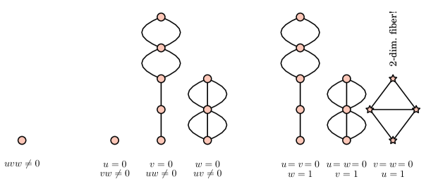
Figure 11: The fiber-divisor-graph $F(O(\sigma),-K)$ of the $2IV^{*}$-fibration over the $7$ torus-orbits $O(\sigma)$, $\sigma\in\Sigma$, in the base ${\mathop{\hbox{}{\mathbb{P}}}\nolimits}^{2}={\mathop{\hbox{}{\mathbb{P}}}\nolimits}_{\Sigma}$.

This asymmetry between the two $IV^{*}$ discriminant components is also visible from the fiber-divisor-graph, see Figure 11. The Kodaira diagram for the $IV^{*}$ degenerate fiber is the extended $\tilde{E}_{6}$ Dynkin diagram, which is folded in two different ways into the fiber-divisor graph over the $v=0$ and $w=0$ component of the discriminant. Over the intersection point $v=w=0$ of the two $IV^{*}$ components of the discriminant the elliptic fiber becomes complex two-dimensional and consists of $4$ irreducible components.

7 Classification of Gauge Groups

7.1 Kodaira Fibers

Having understood the structure of the elliptic fibration in terms of the defining polytope, we can now compute the gauge groups arising from each of the $\sepnum{{.}}{{,}}{}{102581}$ flat toric elliptic fibrations.

Starting with a fibered reflexive lattice polytope $F\subset P$ with $\dim F=2$, $\dim P=4$, that admits a flat fibration over ${\mathop{\hbox{}{\mathbb{P}}}\nolimits}^{2}$ by a toric morphism $\varphi$, we

1. Construct the face fan of $P$,

2. Subdivide the face fan to become a fibration over ${\mathop{\hbox{}{\mathbb{P}}}\nolimits}^{2}$,

3. Pick all integral points of $p\in P$ such that $\varphi(p)$ is zero or contained in a one-dimensional cone of the base ${\mathop{\hbox{}{\mathbb{P}}}\nolimits}^{2}$. In other words, all points that do not map into the interior of a two-cone of ${\mathop{\hbox{}{\mathbb{P}}}\nolimits}^{2}$.

4. Refine the fan further, using these additional rays.

Proceeding this way, we can always resolve the ambient toric variety far enough such that there are homogeneous coordinates that map to the homogeneous coordinates of the base ${\mathop{\hbox{}{\mathbb{P}}}\nolimits}^{2}$, unlike the issue we encountered in eq. (12). It is then straightforward to compute the Weierstrass form of the hypersurface equation and apply Tate’s algorithm Table 1.

Fiber	#
$I_{2}$	53272
$I_{3}$	24303
$I_{4}$	42210
$I_{5}$	18981
$I_{6}$	28782
$I_{7}$	12884
$I_{8}$	15883
$I_{9}$	7424
$I_{10}$	7551
$I_{11}$	3325
$I_{12}$	3629
$I_{13}$	1288

Fiber	#
$I_{14}$	1364
$I_{15}$	519
$I_{16}$	537
$I_{17}$	150
$I_{18}$	207
$I_{19}$	37
$I_{20}$	71
$I_{21}$	15
$I_{22}$	17
$I_{23}$	1
$I_{24}$	11
$I_{27}$	1

Fiber	#
$I^{*}_{0}$	3803
$I^{*}_{1}$	2333
$I^{*}_{2}$	1971
$I^{*}_{3}$	1250
$I^{*}_{4}$	1030
$I^{*}_{5}$	596
$I^{*}_{6}$	477
$I^{*}_{7}$	249
$I^{*}_{8}$	204
$I^{*}_{9}$	92
$I^{*}_{10}$	77
$I^{*}_{11}$	31

Fiber	#
$I^{*}_{13}$	11
$I^{*}_{14}$	13
$I^{*}_{15}$	3
$I^{*}_{16}$	6
$I^{*}_{18}$	2
$I^{*}_{20}$	1
Fiber	#
$II^{*}$	100
$III^{*}$	429
$IV^{*}$	654

Table 2: Kodaira fibers in toric elliptic fibrations and their prevalence.

7.2 Transitions Among Vacua

$h^{21}-h^{11}$	$(h^{11},h^{21})$
270	(2, 272)
228	(3, 231)
204	(4, 208)
192	(3, 195)
190	(4, 194)
184	(5, 189)
174	(6, 180)
168	(5, 173)
165	(6, 171)
162	(3, 165)
160	(7, 167)
158	(4, 162)
156	(5, 161)
153	(8, 161)
150	(4, 154), (6, 156)
147	(6, 153), (7, 154)
144	(7, 151), (9, 153)
142	(2, 144), (8, 150)
140	(4, 144), (7, 147)

$h^{21}-h^{11}$	$(h^{11},h^{21})$
138	(3, 141), (5, 143),
	(8, 146), (10, 148)
136	(6, 142)
133	(7, 140)
132	(4, 136), (13, 145), (15, 147)
130	(2, 132), (7, 137), (8, 138)
128	(5, 133), (8, 136)
126	(2, 128), (6, 132), (18, 144)
124	(5, 129), (11, 135)
122	(4, 126), (6, 128)
120	(3, 123), (5, 125), (7, 127),
	(9, 129), (10, 130), (14, 134),
	(23, 143)
117	(4, 121), (7, 124), (8, 125)
116	(3, 119)
114	(5, 119), (6, 120), (8, 122),
	(9, 123)
112	(4, 116), (5, 117), (7, 119),
	(9, 121), (11, 123)

$h^{21}-h^{11}$	$(h^{11},h^{21})$
-47	(62, 15)
-48	(54, 6), (55, 7), (56, 8),
	(57, 9), (58, 10), (59, 11),
	(60, 12), (61, 13), (62, 14),
	(63, 15), (64, 16), (65, 17)
-50	(63, 13), (65, 15), (66, 16)
-51	(60, 9), (61, 10), (62, 11),
	(63, 12), (64, 13), (66, 15)
-52	(64, 12), (67, 15)
-54	(60, 6), (61, 7), (62, 8),
	(63, 9), (64, 10), (65, 11),
	(66, 12), (67, 13), (68, 14)
-56	(67, 11), (68, 12), (69, 13),
	(71, 15)
-57	(66, 9), (67, 10), (68, 11),
	(70, 13)
-58	(68, 10), (70, 12)

$h^{21}-h^{11}$	$(h^{11},h^{21})$
-60	(67, 7), (68, 8), (69, 9),
	(70, 10), (71, 11), (72, 12),
	(73, 13)
-63	(71, 8), (72, 9), (73, 10),
	(74, 11)
-66	(72, 6), (73, 7), (74, 8),
	(75, 9), (76, 10), (77, 11),
	(78, 12)
-68	(78, 10)
-69	(78, 9), (79, 10)
-72	(79, 7), (80, 8)
-75	(84, 9)
-78	(85, 7), (86, 8), (88, 10)
-84	(90, 6), (91, 7)
-90	(97, 7)
-96	(101, 5)
-108	(112, 4)

Table 3: Hodge numbers $(h^{11},h^{21})$ of flat toric elliptic fibrations over ${\mathop{\hbox{}{\mathbb{P}}}\nolimits}^{2}$ for $h^{21}-h^{11}\geq 112$ and $\leq-47$.

The Hodge numbers of the flat toric elliptic fibrations over ${\mathop{\hbox{}{\mathbb{P}}}\nolimits}^{2}$ are shown in Figures 3 and 4. Let us quickly note some of the salient features. The largest height $h^{11}+h^{21}=2+272$ is attained by a well-known elliptic fibration, the resolution of the weighted projective space ${\mathop{\hbox{}{\mathbb{P}}}\nolimits}^{4}[1,1,1,6,9]$ [2, 32, 4, 3, 38]. The next largest Hodge numbers fall into a sequence $h^{11}=2+k$, $h^{21}=272-29k$ [39]. The factor of 29 is of course the same as in the 6-d anomaly cancellation condition

$$n_{H}-n_{V}=273-29n_{T}.$$ (44)

as any transition between vacua has to preserve the anomaly. However, increasing $n_{T}$ means that the base is blown up, so these sequences are not visible when one restricts to a fixed base. If there are any vacuum transition left after imposing the base, it should hold $h^{21}-h^{11}$ constant. In Table 3, we list the Hodge numbers for the left and right-most cases of the plot Figure 3. While there does not seem to be any pattern to the Hodge numbers with large and positive differences, the Hodge pairs for large negative difference seem to come in sequences $(h^{11}+k,h^{21}-k)$ for consecutive integers $k$. These are visible as vertical lines in Figure 4. Clearly, this is the usual Higgs mechanism giving mass to both a vector and a hyper multiplet. Moreover, large gauge groups are only on the side of large numbers of vector multiplets, $h^{11}\gg 0$. This is nicely illustrated by the fact that the vertical lines in Figure 4 are only visible on the right-hand side of the plot.

A mysterious pattern of the Hodge pairs with $h^{11}\gg h^{21}$ is that they fall into linear sequences $(h^{11}+k,h^{21}-11k)$. For example, the sequence starting with the manifold at the extreme right is

$$\big{(}(112,4),(101,5),(90,6),(79,7),(68,8),(57,9),(46,10),(35,11),(24,12)\big{)}$$ (45)

and all are realized as Hodge numbers of elliptic fibrations. This also holds true for the next right-most manifolds, for example

$$\begin{gathered}\big{(}(97,7),(86,8),(75,9),(64,10),(53,11),(42,12),(31,13),(20,14)\big{)}\\ \big{(}(91,7),(80,8),(69,9),(58,10),(47,11),(36,12),(25,13)\big{)}\\ \big{(}(85,7),(74,8),(63,9),(52,10),(41,11),(30,12),(19,13)\big{)}\end{gathered}$$ (46)

7.3 SU(27) and Anomaly Cancellation

The right-most Hodge pair $(h^{11},h^{21})=(112,4)$ is realized by a single fibered polytope and is in many ways analogous to our simple-most example in Section 4. The lattice polytope is spanned by the vertices

$$P=\operatorname{conv}\big{\{}(-7,-7,-6,-9),(0,1,0,0),(1,0,0,0),(2,2,3,0),(2,2,3,9)\big{\}}$$ (47)

and contains the fiber sub-lattice polytope

$$\operatorname{conv}\big{\{}(-2,-2,-2,-3),(1,1,1,0),(1,1,1,3)\big{\}}\subset P$$ (48)

The polytope $P$ contains 67 integral points:

• The origin,

• One point over the $\vec{u}$ and one over $\vec{v}$ in the base ${\mathop{\hbox{}{\mathbb{P}}}\nolimits}^{2}$ fan,

• 55 points over $\vec{w}$, all being contained in a single two-face $F$,

• and 10 points in the fiber sub-polytope (one of which is the origin).

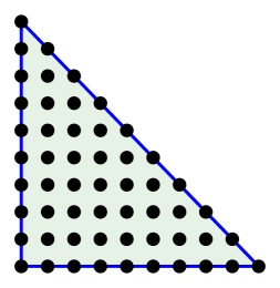
Figure 12: The two-face $F\subset P$ over $\vec{w}$ giving rise to the $I_{27}$ discriminant component.

So the fiber is a cubic in ${\mathop{\hbox{}{\mathbb{P}}}\nolimits}^{2}/(\mathbb{Z}_{3}\times\mathbb{Z}_{3})$, the mirror of a cubic in ${\mathop{\hbox{}{\mathbb{P}}}\nolimits}^{2}$. There are no issues with remaining singularities; One can completely resolve the fan into 243 smooth 4-cones while preserving the fibration structure, and the subdivided fan is a flat toric fibration over ${\mathop{\hbox{}{\mathbb{P}}}\nolimits}^{2}$ with respect to the lattice map

$$\varphi=\begin{pmatrix}0&1&-1&0\\ 1&0&-1&0\end{pmatrix}.$$ (49)

As always, we label the rays of the fan of ${\mathop{\hbox{}{\mathbb{P}}}\nolimits}^{2}$ as in Figure 5. By the arguments above, the toric divisors $u=0$ and $v=0$ do not support a component of the discriminant, only $w=0$ does. The fiber-divisor-graph over $w=0$ is the $\hat{A}_{26}$ extended Dynkin diagram, that is, $27$ nodes in a circle. Just as in Section 4, the extended Dynkin diagram can be seen as the boundary of the two-face of the polytope that sits over $\vec{w}$ in the base fan, see Figure 12. Hence the discriminant component is a split $I_{27}$, leading to a $SU(27)$ gauge theory. Alternatively, one can compute the Weierstrass form of the hypersurface equation and arrive at the same conclusion.

However, in a theory without tensor multiplets the $SU(N)$ gauge group is restricted to $N\leq 24$ by anomaly cancellation [28, 12]. The resolution to this puzzle is that there are extra tensor multiplets coming from a type of codimension-two degeneration that is very generic in toric elliptic fibrations but we have not discussed so far in this paper. In the example under consideration, the toric fiber over $\left<w\right>$ consists of 55 irreducible components, corresponding to the 55 integral points in $F$. The restriction of the anticanonical divisor class is trivial on the 28 internal points, and non-trivial on the 27 points on the boundary of $F$. As we already mentioned before, this is why the hypersurface equation will generically be 27 ${\mathop{\hbox{}{\mathbb{P}}}\nolimits}^{1}$ in complex 2-dimensional toric fiber. The anticanonical divisor class being trivial on a given irreducible toric fiber component means that the hypersurface equation is constant, because that is the only section of a trivial line bundle. But the constant may vary as one moves the fiber around. In particular, the discriminant locus $w=0$ is a ${\mathop{\hbox{}{\mathbb{P}}}\nolimits}^{1}$, so said constant varies in a one-parameter family. Unless this constant along the fiber does not vary at all as one moves in the base direction, there will be certain points of codimension two in the base where the constant vanishes. This means that the fiber of the Calabi-Yau threefold over this point includes a whole toric surface. So while the toric fibration was flat, the elliptic fibration is not because the hypersurface equation identically vanishes over some codimension-two point in the base.

Explicitly, let us divide the set of $66$ homogeneous coordinates into

• $u$ and $v$, the (unique) homogeneous coordinates whose rays map to the base $\vec{v}$ and $\vec{u}$.

• $e_{0}$, $\dots$, $e_{8}$ the homogeneous coordinates on the fiber ${\mathop{\hbox{}{\mathbb{P}}}\nolimits}^{2}/(\mathbb{Z}_{3}\times\mathbb{Z}_{3})$,

• $f_{0}$, $\dots$, $f_{26}$ the homogeneous coordinates corresponding to the points on the boundary of the two-face $F$,

• and $i_{0}$, $\dots$, $i_{27}$ the homogeneous coordinates corresponding to the points in the relative interior of the two-face $F$.

The hypersurface equation contains 13 coefficients $a_{0}$, $\dots$, $a_{12}$. To set notation and for future reference, the hypersurface equation reads in the $e_{\bullet}=f_{\bullet}=1$ patch:

$$\begin{split}p=\;&a_{0}i_{0}i_{1}^{2}i_{2}i_{3}^{3}i_{4}^{2}i_{5}i_{6}^{4}i_{7}^{3}i_{8}^{2}i_{9}i_{10}^{5}i_{11}^{4}i_{12}^{3}i_{13}^{2}i_{14}i_{15}^{6}i_{16}^{5}i_{17}^{4}i_{18}^{3}i_{19}^{2}i_{20}i_{21}^{7}i_{22}^{6}i_{23}^{5}i_{24}^{4}i_{25}^{3}i_{26}^{2}i_{27}+\\ &a_{1}i_{0}^{7}i_{1}^{6}i_{2}^{6}i_{3}^{5}i_{4}^{5}i_{5}^{5}i_{6}^{4}i_{7}^{4}i_{8}^{4}i_{9}^{4}i_{10}^{3}i_{11}^{3}i_{12}^{3}i_{13}^{3}i_{14}^{3}i_{15}^{2}i_{16}^{2}i_{17}^{2}i_{18}^{2}i_{19}^{2}i_{20}^{2}i_{21}i_{22}i_{23}i_{24}i_{25}i_{26}i_{27}+\\ &a_{2}i_{0}^{3}i_{1}^{3}i_{2}^{3}i_{3}^{3}i_{4}^{3}i_{5}^{3}i_{6}^{3}i_{7}^{3}i_{8}^{3}i_{9}^{3}i_{10}^{3}i_{11}^{3}i_{12}^{3}i_{13}^{3}i_{14}^{3}i_{15}^{3}i_{16}^{3}i_{17}^{3}i_{18}^{3}i_{19}^{3}i_{20}^{3}i_{21}^{3}i_{22}^{3}i_{23}^{3}i_{24}^{3}i_{25}^{3}i_{26}^{3}i_{27}^{3}+\\ &a_{3}vi_{0}^{2}i_{1}^{2}i_{2}^{2}i_{3}^{2}i_{4}^{2}i_{5}^{2}i_{6}^{2}i_{7}^{2}i_{8}^{2}i_{9}^{2}i_{10}^{2}i_{11}^{2}i_{12}^{2}i_{13}^{2}i_{14}^{2}i_{15}^{2}i_{16}^{2}i_{17}^{2}i_{18}^{2}i_{19}^{2}i_{20}^{2}i_{21}^{2}i_{22}^{2}i_{23}^{2}i_{24}^{2}i_{25}^{2}i_{26}^{2}i_{27}^{2}+\\ &a_{4}v^{2}i_{0}i_{1}i_{2}i_{3}i_{4}i_{5}i_{6}i_{7}i_{8}i_{9}i_{10}i_{11}i_{12}i_{13}i_{14}i_{15}i_{16}i_{17}i_{18}i_{19}i_{20}i_{21}i_{22}i_{23}i_{24}i_{25}i_{26}i_{27}+\\ &a_{5}v^{3}+\\ &a_{6}ui_{0}^{2}i_{1}^{2}i_{2}^{2}i_{3}^{2}i_{4}^{2}i_{5}^{2}i_{6}^{2}i_{7}^{2}i_{8}^{2}i_{9}^{2}i_{10}^{2}i_{11}^{2}i_{12}^{2}i_{13}^{2}i_{14}^{2}i_{15}^{2}i_{16}^{2}i_{17}^{2}i_{18}^{2}i_{19}^{2}i_{20}^{2}i_{21}^{2}i_{22}^{2}i_{23}^{2}i_{24}^{2}i_{25}^{2}i_{26}^{2}i_{27}^{2}+\\ &a_{7}uvi_{0}i_{1}i_{2}i_{3}i_{4}i_{5}i_{6}i_{7}i_{8}i_{9}i_{10}i_{11}i_{12}i_{13}i_{14}i_{15}i_{16}i_{17}i_{18}i_{19}i_{20}i_{21}i_{22}i_{23}i_{24}i_{25}i_{26}i_{27}+\\ &a_{8}uv^{2}+\\ &a_{9}u^{2}i_{0}i_{1}i_{2}i_{3}i_{4}i_{5}i_{6}i_{7}i_{8}i_{9}i_{10}i_{11}i_{12}i_{13}i_{14}i_{15}i_{16}i_{17}i_{18}i_{19}i_{20}i_{21}i_{22}i_{23}i_{24}i_{25}i_{26}i_{27}+\\ &a_{10}u^{2}v+a_{11}u^{3}+\\ &a_{12}i_{0}i_{1}i_{2}^{2}i_{3}i_{4}^{2}i_{5}^{3}i_{6}i_{7}^{2}i_{8}^{3}i_{9}^{4}i_{10}i_{11}^{2}i_{12}^{3}i_{13}^{4}i_{14}^{5}i_{15}i_{16}^{2}i_{17}^{3}i_{18}^{4}i_{19}^{5}i_{20}^{6}i_{21}i_{22}^{2}i_{23}^{3}i_{24}^{4}i_{25}^{5}i_{26}^{6}i_{27}^{7}\end{split}$$ (50)

and the toric morphism is

$$\Sigma_{P}\to{\mathop{\hbox{}{\mathbb{P}}}\nolimits}^{2},\quad[u:v:e_{\bullet}:f_{\bullet}:i_{\bullet}]\mapsto\Big{[}u:v:\prod e_{\bullet}\prod f_{\bullet}\prod i_{\bullet}\Big{]}$$ (51)

The complex 3-dimensional toric divisor $i_{j}=0$ maps onto the base toric divisor $w=0$, so its fibers are 2-dimensional. For a fixed base point $[u:v:0]$, these are the 28 irreducible components of the toric fiber that correspond to the interior points of the two-face $F\subset P$. The pull-back of the anticanonical class on these toric fiber components is trivial, so the section is constant for fixed $u$, $v$. To determine the constant, we evaluate the hypersurface equation at a generic point, that is, a point in the maximal torus orbit of the toric fiber component. In other words, set

$$i_{j}=0,\quad i_{k}=1~{}\forall k\not=j,\quad e_{\bullet}=f_{\bullet}=1.$$ (52)

Independent of the which of the $28$ $i_{j}$ we set to zero, the hypersurface equation becomes

$$p\big{(}i_{j}=0,~{}i_{k}=1~{}\forall k\not=j,~{}e_{\bullet}=f_{\bullet}=1\big{)}=a_{5}v^{3}+a_{8}uv^{2}+a_{10}u^{2}v+a_{11}u^{3}.$$ (53)

So the constant vanishes at the three solutions of the above cubic. To summarize, there is an $I_{27}$ Kodara fiber over $\{w=0\}\simeq{\mathop{\hbox{}{\mathbb{P}}}\nolimits}^{1}$. Over three points along this discriminant locus, the fiber jumps in dimension and becomes a reducible 2-dimensional toric variety with $28$ irreducible components.

Appendix A Weierstrass Forms

Consider a fibration of lattice polytopes $F\hookrightarrow P$. If the lattice polytope $P$ is reflexive, then the lattice sub-polytope $F$ is reflexive, too. For the purposes of this paper, the fiber polytope will always be $2$-dimensional, that is, one of the $16$ reflexive polygons shown in Figure 13.

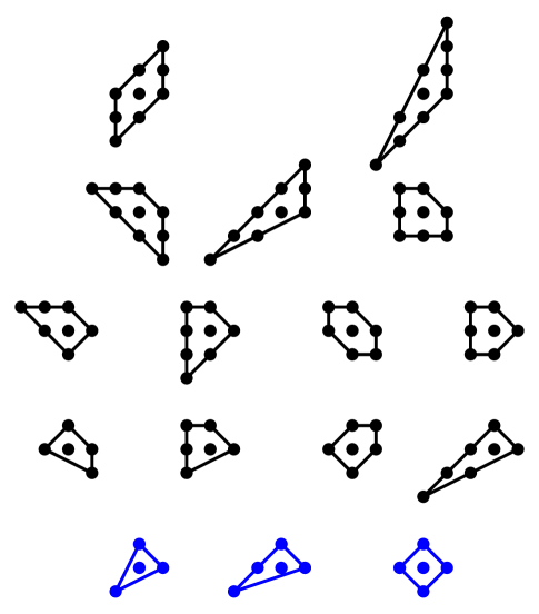
Figure 13: The $16$ reflexive lattice polygons. The $3$ blue polygons at the bottom row are the ones that do not contain a smaller reflexive polygon.

Each lattice polygon defines a face fan and therefore a 2-dimensional compact toric variety. In 2 dimensions, there is a unique maximal cepant desingularization by subdividing the fan such that all lattice points on the boundary of the polygon span a ray of the fan. A generic section of the anticanonical divisor then defines a smooth Calabi-Yau one-fold (that is, a real $2$-torus), irregardless of whether or not one resolves the point-singularities in the ambient toric variety. A smooth $2$-torus can be written as a cubic in ${\mathop{\hbox{}{\mathbb{P}}}\nolimits}^{2}$, where the cubic can be taken to be in Weierstrass from $y^{2}=x^{3}+ax+b$.

In order to identify the discriminant locus of the toric elliptic firations, we need to be able to explictly write the Calabi-Yau hypersurface equation in Weierstrass from. First, however, note that we do not need to give equations for the Weierstrass from for all $16$ reflexive lattice polygons. Since the monomials of the anticanonical hypersurface are the integral points of the dual lattice polygon, we only need to find the transformation to Weierstrass form for the minimal polygons with respect to inclusion. Any strictly larger polygon has a strictly smaller dual polygon, so its anticanonical hypersurface equation is just a specialization where some coefficients are set to zero. In fact, there are $3$ minimal reflexive lattice polytopes, which are shown in blue in Figure 13. The corresponding toric varieties are ${\mathop{\hbox{}{\mathbb{P}}}\nolimits}^{2}$, the weighted projective plane ${\mathop{\hbox{}{\mathbb{P}}}\nolimits}^{2}[1,1,2]$, and ${\mathop{\hbox{}{\mathbb{P}}}\nolimits}^{1}\times{\mathop{\hbox{}{\mathbb{P}}}\nolimits}^{1}$. In the remainder of this appendix, we will discuss these three cases:

• Transforming a cubic in ${\mathop{\hbox{}{\mathbb{P}}}\nolimits}^{2}$ into Weierstrass is well-known, and many computer algebra systems provide an implementation.

• An anticanonical hypersurface in ${\mathop{\hbox{}{\mathbb{P}}}\nolimits}^{1}\times{\mathop{\hbox{}{\mathbb{P}}}\nolimits}^{1}$ is a biquadric eq. (22). The Weierstrass form of the elliptic curve embedded as a hypersurface in ${\mathop{\hbox{}{\mathbb{P}}}\nolimits}^{2}$ is given in eq. (24) [29].

• The remaining case of an anticanonical hypersurface in weighted projective space ${\mathop{\hbox{}{\mathbb{P}}}\nolimits}^{2}[1,1,2]$ will be treated shortly.

Counting only the degrees of the homogeneous coordinates in the fiber fan, the Newton polytope of the hypersurface equation of a toric elliptic fibered Calabi-Yau is always a sub-polytope of the dual polytope of ${\mathop{\hbox{}{\mathbb{P}}}\nolimits}^{2}$ (27 sub-polytopes), the dual polytope of ${\mathop{\hbox{}{\mathbb{P}}}\nolimits}^{1}\times{\mathop{\hbox{}{\mathbb{P}}}\nolimits}^{1}$ (20 sub-polytopes), or of the dual polytope of ${\mathop{\hbox{}{\mathbb{P}}}\nolimits}^{2}[1,1,2]$ (28 sub-polytopes). By embedding the Newton polytope of the hypersurface equation we can then easily compute the Weierstrass form of the hypersurface using the same coordinate transformations as the containing (maximal) reflexive lattice polytope.

It remains to find the Weierstrass cubic representation of an anticanonical hypersurface in ${\mathop{\hbox{}{\mathbb{P}}}\nolimits}^{2}[1,1,2]$.

 
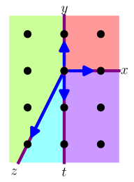
$\vbox{\hbox{\Huge$\downarrow$}}\;\varphi$

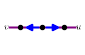
Figure 14: Toric fibration of the resolved weighted projective space $\widehat{{\mathop{\hbox{}{\mathbb{P}}}\nolimits}^{2}[1,1,2]}$ over ${\mathop{\hbox{}{\mathbb{P}}}\nolimits}^{1}$.

Note that there is a single fibration of the resolved ${\mathop{\hbox{}{\mathbb{P}}}\nolimits}^{2}[1,1,2]$ shown in Figure 14, which suggests to take first the discriminant along the fiber directions as in the ${\mathop{\hbox{}{\mathbb{P}}}\nolimits}^{1}\times{\mathop{\hbox{}{\mathbb{P}}}\nolimits}^{1}$ case. The $9$ sections of the anticanonical bundle are

$$H^{0}\left(\widehat{{\mathop{\hbox{}{\mathbb{P}}}\nolimits}^{2}[1,1,2]},-K\right)=\operatorname{span}\big{\{}y^{2},yz^{2}t,xyzt,x^{2}yt,z^{4}t^{2},xz^{3}t^{2},x^{2}z^{2}t^{2},x^{3}zt^{2},x^{4}t^{2}\big{\}}$$ (54)

For convenience, let us switch to inhomogeneous coordinates where $z=t=1$, then the hypersurface equation for an elliptic curve reads

$$C(x,y)=\alpha_{40}x^{4}+\alpha_{30}x^{3}+\alpha_{21}x^{2}y+\alpha_{20}x^{2}+\alpha_{11}xy+\alpha_{02}y^{2}+\alpha_{10}x+\alpha_{01}y+\alpha_{00}$$ (55)

It is quadratic in $y$ with the ordinary quadratic discriminant

$$\beta_{4}x^{4}+\beta_{3}x^{3}+\beta_{2}x^{2}+\beta_{1}x+\beta_{0}=\left(\sum\alpha_{i1}x^{i}\right)^{2}-4\left(\sum\alpha_{i2}x^{i}\right)\left(\sum\alpha_{i0}x^{i}\right).$$ (56)

Again, the quadratic discriminant is a plane quartic as in eq. (22). The coefficients $a$, $b$ of the Weierstrass form $y^{2}=x^{3}+ax+b$ are then again given by the quadratic and cubic projective $GL(2,{\mathbb{C}})$-invariants,

$$\begin{split}a=&-\tfrac{1}{4}\big{(}\beta_{0}\beta_{4}+3\beta_{2}^{2}-4\beta_{1}\beta_{3}\big{)}\\ b=&-\tfrac{1}{4}\big{(}\beta_{0}\beta_{3}^{2}+\beta_{1}^{2}\beta_{4}-\beta_{0}\beta_{2}\beta_{4}-2\beta_{1}\beta_{2}\beta_{3}+\beta_{2}^{3}\big{)}.\end{split}$$ (57)

Bibliography

- [1] J. Tate, “Algorithm for determining the type of a singular fiber in an elliptic pencil,” in Modular functions of one variable, IV (Proc. Internat. Summer School, Univ. Antwerp, Antwerp, 1972), pp. 33–52. Lecture Notes in Math., Vol. 476. Springer, Berlin, 1975.
- [2] C. Vafa, “Evidence for F-Theory,” Nucl. Phys. B469 (1996) 403–418, hep-th/9602022.
- [3] D. R. Morrison and C. Vafa, “Compactifications of F theory on Calabi-Yau threefolds. 1,” Nucl.Phys. B473 (1996) 74–92, hep-th/9602114.
- [4] D. R. Morrison and C. Vafa, “Compactifications of F theory on Calabi-Yau threefolds. 2.,” Nucl.Phys. B476 (1996) 437–469, hep-th/9603161.
- [5] R. Donagi and M. Wijnholt, “Higgs Bundles and UV Completion in F-Theory,” 0904.1218.
- [6] J. Marsano and S. Schafer-Nameki, “Yukawas, G-flux, and Spectral Covers from Resolved Calabi-Yau’s,” 1108.1794. * Temporary entry *.
- [7] S. Katz, D. R. Morrison, S. Schafer-Nameki, and J. Sully, “Tate’s algorithm and F-theory,” JHEP 1108 (2011) 094, 1106.3854.
- [8] R. Miranda, “Smooth models for elliptic threefolds,” in The birational geometry of degenerations (Cambridge, Mass., 1981), vol. 29 of Progr. Math., pp. 85–133. Birkhäuser Boston, Mass., 1983.
- [9] M. Esole and S.-T. Yau, “Small resolutions of SU(5)-models in F-theory,” 1107.0733.
- [10] C. Vafa, “The string landscape and the swampland,” hep-th/0509212.
- [11] V. Kumar, D. R. Morrison, and W. Taylor, “Mapping 6D N = 1 supergravities to F-theory,” JHEP 02 (2010) 099, 0911.3393.
- [12] V. Kumar, D. S. Park, and W. Taylor, “6D supergravity without tensor multiplets,” JHEP 1104 (2011) 080, 1011.0726.
- [13] V. Kumar, D. R. Morrison, and W. Taylor, “Global aspects of the space of 6D N = 1 supergravities,” JHEP 1011 (2010) 118, 1008.1062.
- [14] N. Seiberg and W. Taylor, “Charge Lattices and Consistency of 6D Supergravity,” JHEP 1106 (2011) 001, 1103.0019. * Temporary entry *.
- [15] Y. Hu, C.-H. Liu, and S.-T. Yau, “Toric morphisms and fibrations of toric Calabi-Yau hypersurfaces,” ArXiv Mathematics e-prints (Oct., 2000) arXiv:math/0010082.
- [16] D. A. Cox, “The Homogeneous Coordinate Ring of a Toric Variety, Revised Version,”.
- [17] M. Kreuzer and H. Skarke, “Complete classification of reflexive polyhedra in four dimensions,” Adv. Theor. Math. Phys. 4 (2002) 1209–1230, hep-th/0002240.
- [18] V. Braun, “The 24-Cell and Calabi-Yau Threefolds with Hodge Numbers (1,1),” 1102.4880.
- [19] M. Kreuzer and H. Skarke, “PALP: A Package for analyzing lattice polytopes with applications to toric geometry,” Comput. Phys. Commun. 157 (2004) 87–106, math.na/0204356.
- [20] W. A. Stein et al., Sage Mathematics Software (Version 4.7). The Sage Development Team, 2011. http://www.sagemath.org.
- [21] V. Braun and M. Hampton, Polyhedra module of Sage. The Sage Development Team, 2010. http://sagemath.org/doc/reference/sage/geometry/polyhedra.html.
- [22] K. Kodaira, “On compact analytic surfaces II,” Annals of Math. 77 (1963) 563–626.
- [23] K. Kodaira, “On compact analytic surfaces III,” Annals of Math. 78 (1963) 1–40.
- [24] V. Braun, B. A. Ovrut, T. Pantev, and R. Reinbacher, “Elliptic Calabi-Yau threefolds with Wilson lines,” JHEP 12 (2004) 062, hep-th/0410055.
- [25] V. Braun, M. Kreuzer, B. A. Ovrut, and E. Scheidegger, “Worldsheet Instantons and Torsion Curves, Part B: Mirror Symmetry,” JHEP 10 (2007) 023, arXiv:0704.0449 [hep-th].
- [26] V. Braun, M. Kreuzer, B. A. Ovrut, and E. Scheidegger, “Worldsheet instantons and torsion curves. Part A: Direct computation,” JHEP 10 (2007) 022, hep-th/0703182.
- [27] V. Braun, M. Kreuzer, B. A. Ovrut, and E. Scheidegger, “Worldsheet Instantons, Torsion Curves, and Non-Perturbative Superpotentials,” Phys. Lett. B649 (2007) 334–341, hep-th/0703134.
- [28] D. R. Morrison and W. Taylor, “Matter and singularities,” 1106.3563.
- [29] J. J. Duistermaat, Discrete integrable systems. QRT maps and elliptic surfaces. Springer Monographs in Mathematics. Berlin: Springer. xxii, 627 p., 2010.
- [30] M. Bershadsky et al., “Geometric singularities and enhanced gauge symmetries,” Nucl. Phys. B481 (1996) 215–252, hep-th/9605200.
- [31] A. Grassi and D. R. Morrison, “Anomalies and the Euler characteristic of elliptic Calabi-Yau threefolds,” 1109.0042.
- [32] P. Candelas, E. Perevalov, and G. Rajesh, “F theory duals of nonperturbative heterotic E(8) x E(8) vacua in six-dimensions,” Nucl.Phys. B502 (1997) 613–628, hep-th/9606133.
- [33] P. Candelas, E. Perevalov, and G. Rajesh, “Comments on A, B, C chains of heterotic and type II vacua,” Nucl. Phys. B502 (1997) 594–612, hep-th/9703148.
- [34] P. Candelas, E. Perevalov, and G. Rajesh, “Toric geometry and enhanced gauge symmetry of F theory / heterotic vacua,” Nucl.Phys. B507 (1997) 445–474, hep-th/9704097.
- [35] P. Candelas and H. Skarke, “F theory, SO(32) and toric geometry,” Phys.Lett. B413 (1997) 63–69, hep-th/9706226.
- [36] P. Candelas, E. Perevalov, and G. Rajesh, “Matter from toric geometry,” Nucl.Phys. B519 (1998) 225–238, hep-th/9707049.
- [37] V. Braun, P. Candelas, X. De La Ossa, and A. Grassi, “Toric Calabi-Yau fourfolds, duality between N = 1 theories and divisors that contribute to the superpotential,” hep-th/0001208.
- [38] A. Klemm, P. Mayr, and C. Vafa, “BPS states of exceptional non-critical strings,” hep-th/9607139.
- [39] P. Candelas and A. Font, “Duality between the webs of heterotic and type II vacua,” Nucl. Phys. B511 (1998) 295–325, hep-th/9603170.