The complex behaviour of the microquasar GRS 1915+105 in the $\rho$ class observed with BeppoSAX. II: Time-resolved spectral analysis

Abstract

Context. BeppoSAX observed GRS 1915+105 on October 2000 with a long pointing lasting about ten days. During this observation, the source was mainly in the $\rho$ class characterized by bursts with a recurrence time of between 40 and 100 s.

Aims. We identify five segments in the burst structure and accumulate the average spectra of these segments during each satellite orbit. We present a detailed spectral analysis aimed at determining variations that occur during the burst and understanding the physical process that produces them.

Methods. We compare MECS, HPGSPC, and PDS spectra with several models. Under the assumption that a single model is able to fit all spectra, we find that the combination of a multi-temperature black-body disk and a hybrid corona is able to give a consistent physical explanation of the source behaviour.

Results. Our measured variations in $KT_{el}$, $\tau$, $KT_{in}$, and $R_{in}$ appear to be either correlated or anti-correlated with the count rate in the energy range 1.6-10 keV. The strongest variations are detected along the burst segments: almost all parameters exhibit significant variations in the segments that have the highest fluxes ($pulse$) with the exception of $R_{in}$, which varies continuously and reaches a maximum just before the peak. The flux of the multi-temperature disk strongly increases in the $pulse$ and simultaneously the corona contribution is significantly reduced.

Conclusions. The disk luminosity increases in the $pulse$ and the $R_{in}-T_{in}$ correlation can be most successfully interpreted in term of the slim disk model. In addition, the reduction in the corona luminosity at the bursts might represent the condensation of the corona onto the disk.

1 Introduction

The microquasar GRS 1915+105 (Fender & Belloni 2004) was discovered in 1992 in the hard X-ray band (Castro-Tirado et al. 1992), and later identified with a binary system of an orbital period of about 33 days (Greiner et al. 2001) containing a black hole whose estimated mass is 14.0$\pm$4.4 $M_{\odot}$ (Harlaftis & Greiner 2004). Its distance, evaluated by Mirabel & Rodríguez (1994) and later revised by Fender et al. (1999), is about 12.5 kpc, and a source inclination of 66°– 70°is inferred from the apparent superluminal motion observed in the radio jet (Mirabel & Rodríguez 1994; Fender et al. 1999).

The source has been extensively observed in the X-ray band (Fender & Belloni 2004; Rodriguez et al. 2008; Ueda et al. 2010; Vierdayanti et al. 2010). The X-ray emission is characterized by strong variability with alternating bright bursts and quiet phases. Belloni et al. (2000) classified the X-ray temporal and spectral behaviour of GRS 1915+105 into 12 classes, and Klein-Wolt et al. (2002) and Hannikainen et al. (2005) identified additional sets of variability patterns. As in the case of many black hole candidates (BHC), the spectrum can generally be fitted with at least two components: a first one, dominating at soft X-ray energies ($\leq$10 keV), interpreted in terms of thermal emission, and a second one extending up to several hundreds keV that can be modeled with a power law. The thermal component, which has a higher temperature than in other BHCs, has been interpreted as emission from an accretion disk surrounding the black hole. According to the most accreditated hypothesis, the disk is a thin standard one extending up to a few tens of kilometers from the central source (Fender & Belloni 2004). However, the presence of a slim disk (Abramowicz et al. 1988) has also been advocated to describe some of the spectra observed from this source (Ueda et al. 2009; Vierdayanti et al. 2010; Yadav et al. 1999). The phenomenological power-law model is used to describe a Comptonization component from an optically thick corona above the disk with an electron population containing either thermal or non-thermal particles (Zdziarski et al. 2001) and where energy can be also gained from the gas bulk motion (Titarchuk et al. 1997). In addition to the main spectral components, lower intensity features have occasionally been detected: a Compton reflection from the disk (Zdziarski et al. 2001; Ueda et al. 2009), an iron line present only in a few observations (Feroci et al. 1999; Martocchia et al. 2002, 2006; Ueda et al. 2010).

During the bursts, the main spectral parameters of the thermal component exhibit significant variations, which have been interpreted in term of the emptying and refilling of the inner portion of the accretion disk (Belloni et al. 1997). In agreement with the phenomenology observed in other black holes, the spectral evolution of GRS 1915+105 in all classes can been described as transitions between three separate states, as suggested by Belloni et al. (2000) from the analysis of RXTE observations: a state A with a small time variability where a strong black-body like component with a temperature $>$1 keV dominates the spectrum, a state B with a disk temperature that is higher that in state A and a red-noise time variability on a timescale $>$1 s, and state C where the spectrum is dominated by a power law with a spectral index between 1.8 and 2.6 and white and red noise time variability on a timescale $>$1 s.

The BeppoSAX  satellite observed GRS 1915+105 for about ten days in October 2000. For almost the entire duration of the pointing, the source was in the $\rho$ class according to the classification of Belloni et al. (2000), characterized by quasi-regular bursts with a slow rise and a sharp decrease. We described the time evolution of the source ‘heartbeat’ activity in this period in Massaro et al. (2010, hereafter Paper I), where, on the basis of Fourier and wavelet analysis, we defined the regular and irregular modes of this class. The former mode is characterized by periodograms with one or two prominent peaks and a relatively small variance in the dominant timescale in the wavelet scalograms. In the irregular mode, periodograms exhibit several peaks and wavelet spectra have highly fluctuating timescales. Moreover, pulses of regular series have a number of peaks (multiplicity) that is generally no greater than two, whereas in the bursts of irregular series it increases even to more than four. The two modes were rather clearly separated in time: the irregular mode belongs mainly to the central part of observation (170-375 ks from the beginning), whereas the regular mode was observed in the first and the last portions.

Table 1: Log of the BeppoSAX runs used for the analysis. The columns list the observation codes, the name of the runs, the time in seconds from the starting time of the first observation (20 October 2000 at UT = 21^h 26^m 55^s), the exposure time, the rate observed in the energy range used in the analysis, and the number of run bursts.

Obs. code	Run	Tstart	Exposure	Rate			N burst
		(s)	(s)	(ct s-1)
				MECS	PDS	HP
21226001	A2b	8994.0	2191.0	203.1	39.6	80.2	43
	A3	14727.0	2509.5	203.9	39.2	82.6	53
	A4	20648.0	3152.0	198.0	36.5	80.1	66
	A5	26511.0	2809.5	193.4	35.1	79.1	57
	A6	31928.5	3108.0	191.8	35.4	77.2	64
	A7	37662.0	3156.5	199.2	38.4	79.8	63
	A8b	43402.0	2507.0	197.2	38.4	78.7	62
	A9	49296.0	2952.5	206.1	41.9	82.5	56
212260011	B2b	94999.0	2197.0	207.6	40.6	–	45
	B3	100740.0	2638.5	199.6	38.0	–	55
	B4	107594.0	2008.0	207.6	40.5	–	38
	B5	112199.0	3093.0	212.2	42.5	–	61
	B6	117933.0	3146.5	208.3	40.7	–	65
	B7	123666.5	3122.0	199.3	38.6	–	62
	B8	129400.0	3057.5	203.3	39.2	–	61
	B9b	136123.5	2130.0	205.8	41.0	–	42
	B10	141260.0	2685.0	210.1	41.6	–	52
212260012	C1	181003.0	2198.0	203.4	36.5	83.8	34
	C2	186736.5	2679.0	206.1	41.1	84.0	49
	C3	192470.0	3103.5	206.6	39.2	83.3	61
	C4	198203.5	3121.0	207.3	40.8	83.6	61
	C5	203937.0	3086.5	210.9	43.0	84.6	59
	C6	209816.5	2942.0	211.6	40.2	86.0	59
	C7	215404.0	3067.5	212.5	39.7	88.1	60
212260013	D5b	267005.0	2219.0	215.3	40.9	86.3	43
	D6	272748.0	2675.0	211.3	39.7	85.5	54
	D9	289938.0	3117.5	228.7	39.7	96.5	50
	D10	295671.0	3129.5	227.8	39.0	96.8	45
	D11	301404.5	2987.5	232.2	39.4	98.0	39
	D12	307138.5	3158.0	225.8	40.2	98.4	40
	D13	313230.0	2730.5	216.5	39.1	91.8	40
212260014	E4	358737.5	2666.5	221.3	38.9	91.5	39
	E5	364470.5	3063.0	212.9	37.5	88.7	47
	E6	370204.0	3025.5	204.7	39.6	85.3	42
	E7	375937.0	3112.5	201.9	40.8	83.1	49
	E8	381670.5	3091.0	212.3	42.7	84.8	59
	E10	393136.5	3062.0	215.8	44.2	84.9	55
	E12	405336.0	2361.5	235.1	51.2	94.7	36
212260015	F1	439021.0	2194.0	243.0	52.5	97.9	31
	F2	444735.5	2644.5	231.3	48.9	92.3	40
	F3	450468.0	3020.0	231.9	49.5	93.6	45
	F4	456201.0	3102.0	241.8	51.6	96.3	47
	F6	467752.0	2979.5	237.8	50.6	95.1	49
	F7	473400.5	3099.0	234.3	49.4	93.0	51
	F8	479133.5	2934.5	233.6	49.2	92.5	46
	F9	485200.0	2744.5	229.6	48.7	91.5	44
	F17	530768.0	2578.0	244.3	51.9	97.8	36
212260016	G3	547929.0	3070.5	243.0	52.1	–	46
	G4	553723.5	3026.0	234.1	48.4	–	50
	G5	559395.0	3072.5	235.6	48.9	–	53
	G6b	566000.5	2153.0	244.1	53.0	–	33
	G7	571145.0	2781.5	230.0	48.4	–	42

In this paper, we present a time-resolved spectral analysis of a large fraction of the data series of Paper I with the principal aim of obtaining more information on the spectral changes associated with the bursts. We included, in addition, results from a short simultaneous RXTE observation. A spectral analysis of the $\rho$ mode was presented by Taam et al. (1997) and Vilhu & Nevalainen (1998) using data from RXTE. Nevertheless, a complete study of the burst processes, which is typical of the $\rho$ class, is not yet available (while this paper was under the referee process Neilsen et al. (2011) published their results on the analysis of $\rho$ mode spectra observed with RXTE).

In our analysis, we applied to the data set several spectral models that have been found to closely fit the energy spectral distributions of GRS 1915+105 in various variability classes; we identified those able to provide a satisfactory general description of the spectra, and then studied the variations in their main properties. Moreover, we present the results of a much shorter simultaneous RXTE observation.

Data and selection procedures are illustrated in Sects. 2 and 3, the spectral analysis is presented in Sect. 4, and the time evolution of the spectral parameters is given in Sect. 5. The analysis of RXTE data is described in Sect. 6 and the physical discussion of the results is provided in Sect. 7.

2 Observation and data reduction

BeppoSAX observed the GRS 1915+105 in 2000 from October 20 (MJD 51837.894) to October 29. As in Paper I, we used the data obtained with the Medium Energy Concentrator Spectrometer (MECS), operating in the 1.3–10 keV energy band (Boella et al. 1997), and the Phoswich Detector System (PDS) operating in the 15–300 keV energy band (Frontera et al. 1997). Furthermore, we considered the data obtained with the High Pressure Gas Scintillation Proportional Counter (HPGSPC; Manzo et al. 1997), which worked in the nominal energy band 4–120 keV, and covers the gap between the two other instruments.

Data retrieved from BeppoSAX archive at the ASI Science Data Center are organized into observations containing several satellite orbits with a period of $\sim$96 m. In Paper I, we divided the observations into runs, each corresponding to a continuous observing period, and named the runs with capital letters and sequential numbers. In this paper, we present the spectral analysis performed over runs having exposure times greater than 2000 s in order to have, in all instruments, a number of counts sufficient to confine the spectral parameters. Table 1 lists these 52 runs, together with the code of the observation from where they were extracted, the time in seconds from the starting time of the first observation (20 October 2000 at UT = 21^h 26^m 55^s), the exposure, the rate of each instrument in the energy range considered for the spectral analysis (1.6–10 keV for the MECS, 8–30 keV for the HPGSPC and 15–150 keV for the PDS), and the number of bursts detected in each series.

The extraction and reduction procedures for the MECS and PDS data were already described in Paper I; for HPGSPC, we used the latest distributed version of SAXDAS (v2.3.1) and applied the standard selection criteria. The tool used to extract HPGSPC spectra (hpproducts v3.1.1) produces some failure in the gain correction of data from observations 212260011 and 212260016, which were consequently excluded from the analysis.

The MECS background, estimated from high Galactic latitude ‘blank’ fields accumulated in the same region of the detectors, is neglected, as it has a count rate of a level 2.6$\times$10^-2 c s^-1, which is much lower than the typical source flux, even in the faintest states. Both the PDS and HPGSPC background were obtained from simultaneous measurements thanks to the standard operational rocking mode.

Our spectral analysis was performed with XSPEC v.11 using the response matrices, that are available from the BeppoSAX archive. We restricted the spectral analysis of HPGSPC data to the energy range 8–30 keV where the response matrix is more accurate. The MECS-PDS intercalibration factor was fixed to 0.85, which is its average value in the range 0.83-0.89 for point sources of high count rate, and the MECS-HPGSPC factor was limited to vary within the range 0.9-1.1 to take into account the discrepancy in the flux measured by the two instruments. We found that HPGSPC measured a flux $\sim$7% higher than the MECS.

The errors in the values of the best-fit parameters reported throughout the paper and in the tables correspond to a 1 $\sigma$ confidence level for a single parameter, unless explicitly stated.

3 Burst “anatomy” and count rate variations

In Paper I, we distinguished three main phase intervals or segments of the burst profile and investigated the time evolution of the count rates for each of them. The most prominent feature is the pulse, which generally consist of several short peaks. Prior to the pulse, there is the slow leading trail (hereafter SLT), which is also called the ‘shoulder’ in the literature, during which the count rate increases much slower than in the pulse. There is no clear separation between these two components, and we took it at the time where the count rate reached the level of the FWHM of the pulse, which was evaluated by means of a Gaussian best-fit. Between the end of the pulse and the beginning of the SLT, the count rate reaches its lowest level that can be considered as a baseline upon which bursts are superposed. We defined a time interval of three seconds where it is possible to estimate this baseline level (hereafter BL corresponding to the first three seconds of the red segment of the light curve shown in Fig. 1) and found that BL remained remarkably stable in each individual time series (see Paper I for more details). In the spectral analysis, we essentially followed this division and introduced a finer partition.

The analysis of the BL spectra gave parameters in agreement, within the errors, with those of the SLT ones, and owing to the lower quality statistics, we did not consider BL as a separate segment. The signal in the entire SLT is strong enough to divide this component into two parts of equal length, hereafter called SLT-1 and SLT-2, respectively, which are plotted using data points of different colors in Fig. 1, where a short segment of the series A3 is reported as an example. The same colors are also used in the other figures to permit an easier identification of the various time segments. We also divided the pulse into two equal time intervals, namely P-1 and P-2, which are indicated in Fig. 1 and in subsequent figures by blue and cyan data points, respectively. An even finer segmentation to enable us to analyze individual peaks was not possible because the peak shape and duration is highly variable from burst to burst. Finally, the ending part of the pulse to the initial minimum of SLT was taken as a fifth segment, marked in Fig. 1 with light grey points, and labeled FDT corresponding to Final Decaying Trail. The starting and ending times of these parts in each burst were evaluated by means of the same procedure described in Paper I. For each data series of MECS, HPGSPC (whenever available), and PDS, we accumulated five spectra, each of them corresponding to the integral of a selected part of the burst.

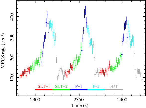
Figure 1: A snap shot of the light curve in the entire MECS energy range of the series A3. Red and green data points indicate the SLT-1 andSLT-2 intervals, blue and cyan points are for P-1 and P-2, and grey points indicate the ending part of the burst (FDT).

The variations in the count rates of the various components in the course of this long pointing were analysed in detail in Paper I. However, to take into account the finer segmentation of the bursts’ profile introduced during the spectral analysis, we again tracked the behaviour of each part to highlight any possible differences from the results presented in Paper I. We considered the same time segmentation of the whole dataset in three intervals introduced in Paper I: interval I from the start time to 1.7$\times$10⁵ s, interval II from this time to 3.8$\times$10⁵ s, and the last interval III is from 4.0$\times$10⁵ s to 6.0$\times$10⁵ s. In particular, the second interval is characterized by the presence of the irregular mode detected in the timing analysis (Paper I), and the last interval corresponds to the final high state after the rapid increase in count rate detected between 3.8$\times$10⁵ s and 4.0$\times$10⁵ s. Figures  2 and  3 show the average rate for the five portions of the bursts for each series in the 1.6–10 keV (MECS) and 15–100 keV (PDS) energy ranges, respectively.

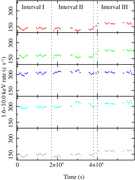
Figure 2: Time history of MECS (1.6–10 keV) count rates for the five segments identified along the bursts. Top to bottom: SLT-1 (red), SLT-2 (green), P-1 (blue), P-2 (cyan), and FDT (grey). Vertical dashed lines mark the main intervals of the observation.

As already discussed in Paper I, the evolution of the count rates is not the same for the different parts of the bursts. The behaviours of SLT-1, SLT-2, and FDT are similar in the MECS and PDS data sets, and their count rates undergo a significant increase between 380 ks and 400 ks with nearly stable levels before and after this transition, as was also found for the BL level (see the lower panel of Fig.15 in Paper I).

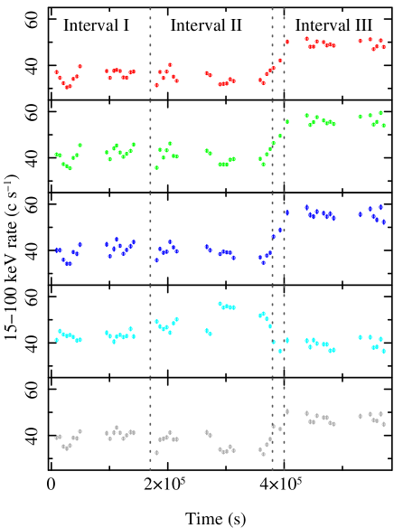
Figure 3: Time history of PDS (15–100 keV) count rates for the five segments identified along the bursts. Top to bottom: SLT-1 (red), SLT-2 (green), P-1 (blue), P-2 (cyan), and FDT (grey). Vertical dashed lines mark the main intervals of the observation.

In the MECS data, the count rates of P-1 and P-2 remain quite stable during the entire length of the observation, without any indication of a step increase. We note that the relative pulse contribution in the MECS range is higher in the first 400 ks of observation (before the step increase) as shown in Fig. 15 of Paper I, where we present the difference of the rate with respect to the BL level. In the PDS data, the rate variation among the five segments is lower than in the MECS (the largest difference is 1.7 compared to 2.5 in the MECS), and the presence of the peak contribution is only evident in P-2, for which there is a strong increase in the rate during the first 400 ks with a bump in the central part of the pointing where the source was in an irregular mode. The hardening of P-2 during the irregular mode was already reported in Paper I, where we noted that PDS peaks were clearly apparent only in the final part of the pulse, while in the regular series they were not so high. In summary, there is a strong correlation between the MECS and the PDS rate, which weakens at the $pulse$, where the MECS rate is almost constant.

The spectral variations within the five segments correspond to cyclical changes in the state defined by Belloni et al. (2000): the source is mainly in state C in the SLT, moves to A in P-1, then to B in P-2, and, finally, returns to C in the FDT section.

4 Spectral analysis

As simple spectral models had been shown not to give acceptable fits over an energy range from a fraction of a keV to about one hundred keV, we considered composite models. The majority of the models that we studied had indeed been previously used to investigate this source, although for different brightness states and variability classes. These models include the emission from a standard optically thick accretion disk to reproduce the spectrum up to about 15 keV (diskbb in XSPEC Mitsuda et al. 1984), and, at higher energies, they consider other spectral functions that generally have a significant contribution also at lower energies. We tried several models (listed in Appendix A) that interpret the expected spectral shape either with a combination of phenomenological functions or with laws based on theoretical descriptions of a corona-accretion disk system.

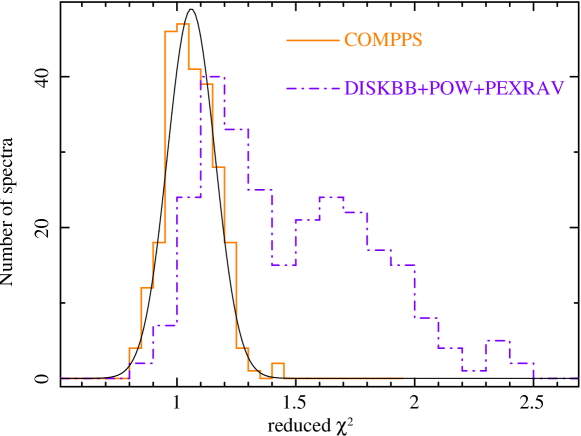
Figure 4: Frequency histograms of the reduced $\chi^{2}$ for all spectra of the “good model” (continuous orange line) and of model $iv$ described in Appendix A (dashed line) compared with the expected distribution evaluated by a MonteCarlo simulation (black line).

We required that the same spectral model was able to fit all the 52 spectra of each segment by changing only the values of the parameters. To test the consistency of the model with the data, we compared the frequency distribution of the reduced $\chi^{2}$ with the expected parent distribution. This was evaluated from 10000 simulated distributions each generated by randomizing a set of 52 values from the $\chi^{2}$ functions corresponding to the degree of freedom of each observed spectrum. We found that a model closely fitting all spectra has an expected distribution of the reduced $\chi^{2}$ given by a Gaussian-like function centered on 1.00$\pm$0.02 that has a standard deviation of $\sigma$=0.10$\pm$0.01. As a result of our fits, we found that the reduced $\chi^{2}$ distribution has the expected width (0.10$\pm$0.01), but the mean (1.05$\pm$0.01) is shifted even if compatible with the expected one to within two standard deviations. This shift is mainly caused by the highest quality data statistics (such as those of the $pulse$) and may be produced by residual systematics originating either from local detector features at the maximum level of 5% (such as the 4.78 keV residual in the MECS spectra) or from the uncertainty in the intercalibration factors ($\sim$3%) fixed for the PDS to 0.85 (see Sect. 2). This effect cannot be properly treated within XSPEC, where systematics are introduced as a single factor over the entire fitting range. To take this effect into account, we compared our $\chi^{2}$ distribution with a Gaussian centered on 1.06 and the compatibility of the resulting distributions with the expected one was confirmed by means of a Kolmologov-Smirnov test.

                                                                                         

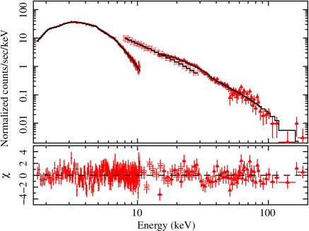
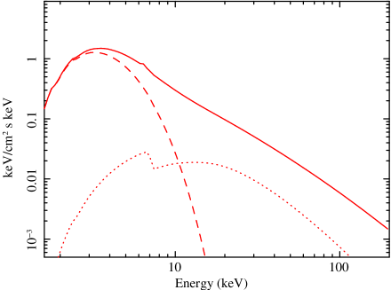
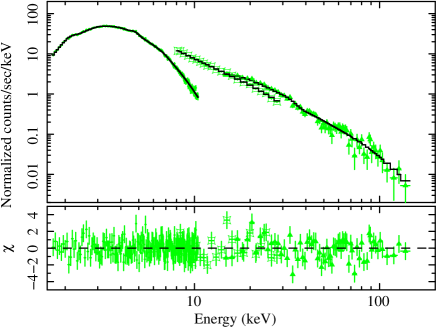
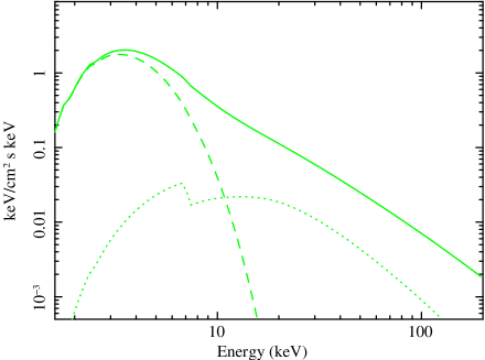
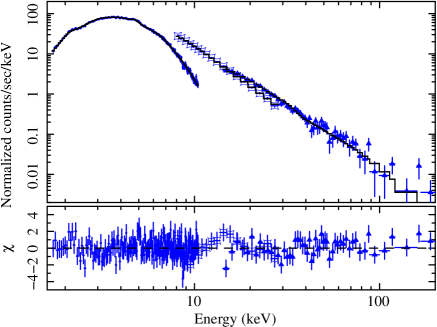
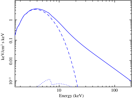
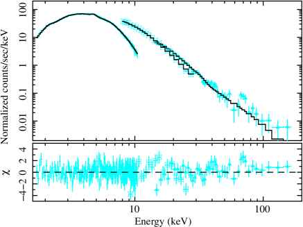
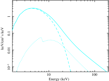
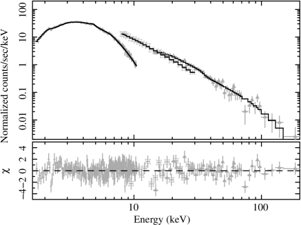
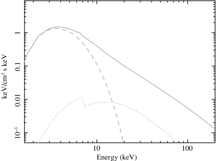
Figure 5: Left panels: Data and fitting model plus residuals for spectra in run E7. Right panels: Best-fit models (continuous line) with the relative spectral components: disk (dashed line) and Compton reflection (dotted line).

We found that the “good model” that most closely describes the source behaviour during the burst and provides a consistent physical interpretation is the standard disk plus a corona that contains an hybrid population of electrons including both thermal and non-thermal distributions (Poutanen & Svensson 1996). The code relative to this model implemented in XSPEC (compps) includes, together with emission from the multi-temperature disk and corona, the Compton reflection from gas whose temperature and ionization status can be set as fitting parameters. It provides acceptable best-fits to the spectra of all data sets and the reduced $\chi^{2}$ distribution is compatible with the expected one within only one standard deviation as shown in Fig. 4, where the compps $\chi^{2}$ distribution is compared with the one relative to the model $iv$ (top panel) described in Appendix A. The model $v$ in Appendix A (diskbb+pow+bbody) also provides fully acceptable best-fits, without any prominent features in the residuals, for the spectra of all data sets. However, as explained in Appendix A, no simple physical interpretation can be given for the black-body component, and therefore it was not considered in the subsequent analysis.

In the compps fits, the electron distribution is assumed to be thermal below a Lorenz factor $\gamma_{min}$ above which energies are distributed with a power law spectrum of index $\Gamma$ up to a Lorenz factor $\gamma_{max}$ fixed at 10³ (Zdziarski et al. 2005). The values of $\gamma_{min}$ and $\Gamma$, which were free to vary during first sets of fitting, were found to maintain almost constant values ($\gamma_{min}$: mean 1.3, rms 0.7; $\Gamma$: mean 4.6, rms 1.6) in all the observations and in the various segments and were then fixed to their average values. The $\gamma_{min}$ closely agrees with the results obtained by Zdziarski et al. (2005) for the analysis of RXTE$+$OSSE observations, while, $\Gamma$ is fixed to a value slightly larger or marginally compatible with those from previous measurements (Zdziarski et al. 2005; Ueda et al. 2010).

The disk, surrounded by a spherical corona (param $geom$=0 in XSPEC), extends to between 10 and 1000 Schwarzschild radii with an inclination of $\theta$=70°. Compton reflection from a non-rotating disk (param Betor10=-10 in XSPEC) with a gas temperature of 10⁶ K and a low level of ionization (param $\xi$=0) is also taken into account.

A reduction in the free parameters led to a broader $\chi^{2}$ distribution that was still compatible with the expected one (see Fig. 4). The free-fitting parameters were thus: the absorbing column density ($N_{\rm H}$), the temperature ($kT_{el}$), and the optical depth ($\tau$) of the corona, then the temperature ($kT_{in}$) and the apparent inner radius ($R_{in}$) of the accretion disk, and the solid angle of the cold reflecting matter to the illuminating source ($\Omega$) expressed in units of 2$\pi$. The values of $R_{in}$ are computed from the normalization of the model, $K$, using the relation $K=(R_{in}[{\rm km}]/D[10\,{\rm kpc}])^{2}\times cos(\theta)$, where $D$ is the distance (12.5 kpc). They are practically equivalent (to within a few percent) to the ones computed using the formula given by Kubota & Makishima (2004) that, assuming isotropic radiation, takes into account the conservation of the photon number in the Comptonization process.

The spectral fittings and residuals for the five segments of the series E7 are shown in the left panels of Fig. 5; their relative models plus components are plotted in the right panels of the same figure.

4.1 The iron line

The detection of a fluorescence K$\alpha$ iron line from GRS 1915+105 has been reported on several occasions (Martocchia et al. 2002; Zdziarski et al. 2005; Martocchia et al. 2006; Ueda et al. 2010) and, more recently, by Titarchuk & Seifina (2009). In particular, Martocchia et al. (2002) from the detection of a strong line found evidence of relativistic effects in a black hole environment.

We searched for the presence of the K$\alpha$ iron line by including in the adopted model a Gaussian profile, whose central energy was allowed to vary across the range between 6.3 keV and 7.1 keV and whose width was fixed to 0.1 keV. No significant line was observed in any of the analyzed spectra with a maximum detection of 2.5 $\sigma$ only in a few spectra and a 3$\sigma$ upper limit of $\sim$50 eV to the EW.

4.2 The low energy absorption

The low energy absorption of GRS 1915+105 is complex and variable (Belloni et al. 2000; Lee et al. 2002; Martocchia et al. 2006; Yadav 2006; Ueda et al. 2009, 2010; van Oers et al. 2010). The values of the equivalent column density $N_{\rm H}$ obtained from the analysis of X-ray data ranges between 2$\times 10^{22}$ and 16$\times 10^{22}$ cm^-2 (Greiner et al. 1996; Taam et al. 1997; Trudolyubov 2001; Martocchia et al. 2002; Lee et al. 2002; Yadav 2006; van Oers et al. 2010) and are generally higher than the values derived from the 21 cm hydrogen line emission along the line of sight (4.7$\pm$0.2$\times 10^{22}$ cm^-2; Chaty et al. 1996) ($\geq 1.8\times 10^{22}$ cm^-2; Dickey & Lockman 1990). These results indicate that there is a composite local absorber containing materials in grains whose characteristics have been derived with Chandra observations (Lee et al. 2002; Ueda et al. 2009).

Since our data are relative to an instrument of moderate energy resolution, and a low energy boundary at $\sim$2 keV, we adopted the XSPEC wabs function assuming standard solar abundance from Anders & Grevesse (1989). No significant variation in the absorbing column was discerned during the ten days of observations. However, we found a rather weak increase in the column density at the peak: the $N_{\rm H}$ varied between 4.3$\times 10^{22}$ cm^-2 in the $SLT$ and 5.4$\times 10^{22}$ cm^-2 in the pulse (see Table 2). Fixing the $N_{\rm H}$ to an intermediate value resulted only in a small worsening of the $\chi^{2}$ distribution without affecting the values of the other parameters. In particular, fixing to 5.0$\times 10^{22}$ cm^-2 the $N_{\rm H}$ of the P-2 spectra, differences smaller than 10% were measured for the disk parameters and values that were compatible to within 2$\sigma$ for the corona ones.

Following Ueda et al. (2010), we evaluated the contribution of the halo produced by dust scattering to the MECS spectra below 3 keV. We found that it produces about 10% of the emission assuming the fractional intensity derived for GX 13$+$1 (Smith et al. 2002). This could account for the apparent variability of $N_{\rm H}$ on a long timescale, but the scattered flux is not expected to vary during the period 40-100 s coherently with the burst, where the time delay respect to the source emission is about 100 hours (Ueda et al. 2010).

We also fitted our spectra with a more complex absorption model (tbvarabs in XSPEC) by fixing the abundances to the values obtained by Lee et al. (2002) and Ueda et al. (2009), and in both cases a broader $\chi^{2}$ distribution centered at $\sim$1.2 was obtained. Leaving the abundances free to vary produced poorly constrained values. No clear explanation can be found for this result that may also be due to the time variability of the absorber.

5 Evolution of the spectral parameters

We analyzed the variations in the best-fit spectral parameters in the course of the observation to search for possible correlations between them and with the changes in the mean source luminosity. We present our results in term of the two main components of the model: the disk and the corona.

For the three intervals we evaluated the average values of the parameters of each component and their rms, as given in Table 2, to take into account the variability, which is also listed in the table as uncertainties. The time evolution of the parameters for the corona and the disk component are shown in Figs. 6 and  7, respectively. Moreover, at the end of the fitting procedure, we derived the disk contribution to the total flux by setting $\tau$ and $\Omega$ to zero, and equated the contribution of the corona to the difference. Non-thermal electrons are responsible for $\sim$30% in SLTs and 15% in the pulse of the coronal emission as evaluated by setting the parameter $gmin$ to a negative value (i.e., purely thermal case).

The reflection component was detected with a significance higher than 3$\sigma$, in the SLT, while no reflection is observed in the pulse. Its contribution to the total flux is always lower than 10%. The solid angle has almost no significant variations either with time or segment. In particular, we obtained $\Omega$=1.2$\pm$0.3 and $\Omega$=1.6$\pm$0.3 for SLT-1 and SLT-2, respectively, for the average and rms value during the ten days of observations. These values are higher than expected based on the upper limit to the equivalent width of the narrow iron-K line ($\Omega\leq$0.5), but, when this parameter is constrained to values lower then the upper limit, the maximum ($\Omega$=0.5) for all spectra is found. Several different values are given in the literature for the reflecting solid angle, ranging from 0.1 to 2 (Feroci et al. 1999; Zdziarski et al. 2005; Martocchia et al. 2006; Ueda et al. 2009; van Oers et al. 2010), that could be related to the spectral state of the source (Sobolewska & Życki 2003). Results obtained from our analysis are compatible with the ones presented by Sobolewska & Życki (2003) and Zdziarski et al. (2005) for other variability classes. However, the low iron abundance that we used for our fitting could lead to an overestimate of the intensity of the reflection component.

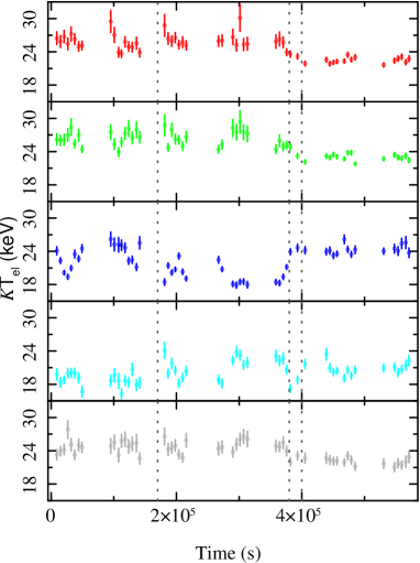
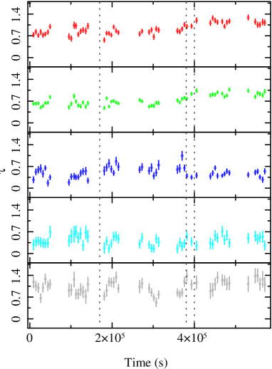
Figure 6: Corona: Temperature (top figure) and optical depth (bottom figure) of the thermal component of the electron population in the corona vs time in the five segments.

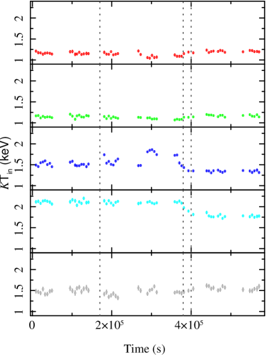
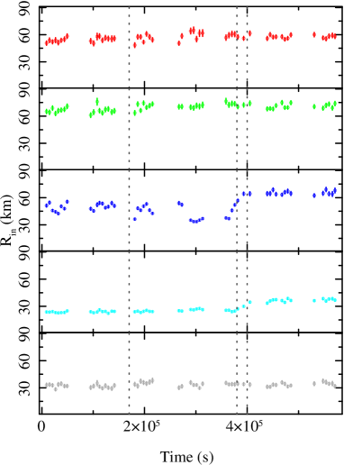
Figure 7: Multi-temperature black-body disk: Disk temperature (top figure) and apparent inner radius (bottom figure) vs time in the five segments.

The variations in $kT_{el}$, $\tau$, $kT_{in}$, and $R_{in}$ were found to be either correlated or anti-correlated with the 1.6-10 keV MECS and 15-100 keV PDS rates for the majority of the segments. These parameters have almost constant values in the intervals I and III ($regular$ mode) with a significant change in the mean values occurring in correspondence with the increase in the count rate. During interval II ($irregular$ mode), the values are remarkably similar to those of interval I, but have a larger variance.

The strongest variations are detected for the segments, as shown in Figs. 8 and  9, where the averages for the three intervals are plotted with different line styles (a solid line for interval I, a dashed line for II, and a dotted line for III). The figures also show the 0.01–200 keV flux in units of 10^-9 erg cm^-2 s^-1 in the bottom panels computed by extrapolating to lower energy the best-fit model. The parameters have very similar values in SLT-1 and SLT-2, while they exhibit significant variations in the pulse with the exception of $R_{in}$, which varies throughout all segments and reaches a maximum in SLT-2 as previously observed by Vilhu & Nevalainen (1998). The flux of the multi-temperature disk strongly increases during the pulse, and simultaneously the corona contribution reduces significantly with respect to the values detected in SLT. Moreover, the corona increases its emission by 40-50% from interval II to interval III, while smaller variations (20-30%) are observed in the disk flux during the three intervals, suggesting that the increase in the rate after 4.0$\times$10⁵ s is caused mainly by this component.

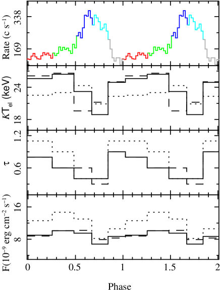
Figure 8: Corona: Variability of the spectral parameters along the segments. The electron temperature is shown in the second panel, the optical depth in the third, and the 0.01-100 keV flux in the bottom one. Interval I is represented with a solid line, II with a dashed line, and III with a dotted line. The top panel shows the MECS rate for comparison; two bursts are shown for clarity.

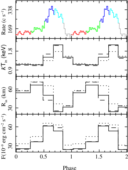
Figure 9: Multi-temperature black-body disk: Variability of the spectral parameters along the segments. The temperature is shown in the second panel, the apparent inner radius in the third and the the 0.01-100 keV flux calculated by setting $\tau$ and $\Omega$ to 0 in the bottom one. Interval I is represented with a solid line, II with a dashed line and III with a dotted line. The top panel shows the MECS rate for comparison; two bursts are shown for clarity.

The total luminosity of the source, for a distance of 12.5 kpc, was also computed in the 0.01–200 keV range as $L_{tot}=L_{disk}+L_{corona}$, assuming isotropic emission for both components and deriving $L_{disk}$ by setting both $\tau$ and $\Omega$ to 0. The source luminosity changes from $\sim$50% of the Eddington luminosity (for a black hole mass of 14 $M_{odot}$) to 100% (or slightly above it) in the pulse as shown in the second panel of Fig. 10. In the third and fourth panels of the same figure, the fraction of the total luminosity versus (vs) segment for the disk and the corona are also shown. It is evident that the increase in the pulse flux is due to the disk contribution, and that a higher percentage of photons is Comptonized by the corona after 400 ks.

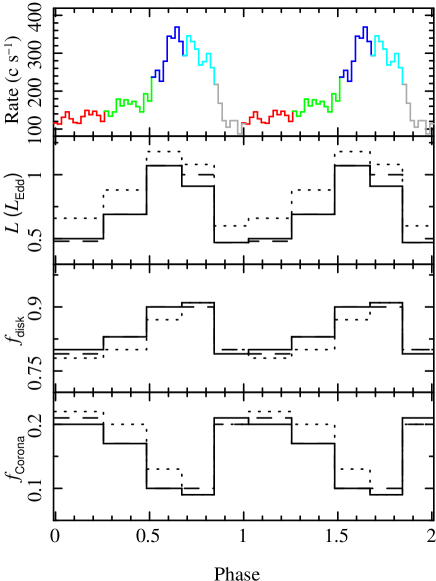
Figure 10: Evolution of the total luminosity in units of Eddington luminosity (second panel) for the considered burst segments. The fraction of the total luminosity for the disk and the corona are shown in the third and fourth panels, respectively. Interval I is represented with a solid line, II with a dashed line, and III with a dotted line. The top panel shows the MECS rate for comparison; two bursts are shown for clarity.

Table 2: Average best-fit parameters for the BeppoSAX spectra fit with the “good model” in the three intervals I (0-170 ks), II (170-380 ks), and III (400-600 ks). The last section of the table shows the results relative to the two RXTE spectra.

	Disk			Corona
	$kT_{in}$	$R_{in}$	F∗	$kT_{el}$	$\tau$	F∗	N${}_{\rm H}^{**}$
	(keV)	(km)		(keV)
Interval I
SLT-1	1.17$\pm$0.02	54.0$\pm$2.1	25.7$\pm$1.3	25.6$\pm$1.3	0.8$\pm$0.1	9.0$\pm$0.9	4.64$\pm$0.06
SLT-2	1.15$\pm$0.02	66.2$\pm$2.5	36.8$\pm$1.5	26.4$\pm$1.1	0.6$\pm$0.1	10.1$\pm$1.3	4.98$\pm$0.04
P-1	1.51$\pm$0.04	50.0$\pm$3.7	62.0$\pm$3.3	23.2$\pm$1.9	0.4$\pm$0.1	9.5$\pm$0.7	5.27$\pm$0.08
P-2	2.10$\pm$0.07	24.0$\pm$1.4	53.6$\pm$1.5	18.9$\pm$1.1	0.4$\pm$0.1	6.8$\pm$0.8	4.86$\pm$0.08
FDT	1.51$\pm$0.05	31.3$\pm$1.8	24.0$\pm$1.6	24.9$\pm$1.2	0.9$\pm$0.2	8.7$\pm$0.6	4.31$\pm$0.10
Interval II
SLT-1	1.13$\pm$0.05	57.0$\pm$4.2	24.7$\pm$1.7	26.1$\pm$1.2	0.8$\pm$0.1	8.8$\pm$0.8	4.6$\pm$0.1
SLT-2	1.11$\pm$0.02	70.9$\pm$3.1	36.7$\pm$1.9	26.6$\pm$1.4	0.6$\pm$0.1	10.1$\pm$0.8	5.0$\pm$0.1
P-1	1.66$\pm$0.13	42.2$\pm$7.1	61.5$\pm$2.8	19.6$\pm$1.6	0.6$\pm$0.1	10.2$\pm$0.7	5.2$\pm$0.1
P-2	2.07$\pm$0.07	25.3$\pm$1.1	58.4$\pm$4.8	21.2$\pm$1.8	0.3$\pm$0.1	7.9$\pm$0.5	5.0$\pm$0.1
FDT	1.46$\pm$0.07	33.5$\pm$2.3	24.2$\pm$2.0	25.0$\pm$1.0	0.9$\pm$0.2	8.3$\pm$0.8	4.4$\pm$0.1
Interval III
SLT-1	1.21$\pm$0.02	57.5$\pm$2.1	33.6$\pm$0.8	22.5$\pm$0.5	1.1$\pm$0.1	12.6$\pm$0.5	4.83$\pm$0.07
SLT-2	1.17$\pm$0.02	71.2$\pm$2.4	45.3$\pm$0.9	23.0$\pm$0.5	0.9$\pm$0.1	14.7$\pm$0.8	5.10$\pm$0.05
P-1	1.35$\pm$0.02	65.2$\pm$2.0	67.1$\pm$1.3	24.3$\pm$0.8	0.4$\pm$0.1	13.0$\pm$0.7	5.39$\pm$0.05
P-2	1.78$\pm$0.03	36.4$\pm$1.5	63.3$\pm$2.1	20.9$\pm$1.0	0.4$\pm$0.1	8.2$\pm$0.8	5.15$\pm$0.05
FDT	1.56$\pm$0.04	33.3$\pm$1.9	31.0$\pm$0.8	22.3$\pm$0.7	1.1$\pm$0.1	10.6$\pm$0.6	4.53$\pm$0.09
RXTE
SLT	1.34$\pm$0.02	60$\pm$3	56.2$\pm$1.0	20.5$\pm$0.3	1.06$\pm$0.06	15.9$\pm$0.3	5.7$\pm$0.3
P	1.50$\pm$0.03	56$\pm$1	74.6$\pm$3.1	21.2$\pm$0.4	0.60$\pm$0.09	15.4$\pm$0.1	5.3$\pm$0.3
∗Flux in the range 0.01-200 keV in unit of 10-9 erg cm-2 s-1
∗∗in unit of 1022 cm-2

6 RXTE simultaneous observation

RXTE observed GRS 1915+105 a few times during the BeppoSAX long observation. We extracted the data from observation 50405-01-04-00, made on 2000 October 27 06:28-09:25 UT. The starting time of this data series was 550830.0 s after the beginning of the BeppoSAX pointing. The exposure times and count rates were 2480 s and 3033.7 ct s^-1 for the PCA, and 805 s and 28.3 ct s^-1 for HEXTE, respectively. Spectral data were available only with time resolution of 16 seconds, we then defined from the PCA light curve (see bottom panel of Fig. 11) two intervals, SLT (9000-15000 ct s^-1 ) and P ($>$15000 ct s^-1), where were as close as possible to the BeppoSAX finer selection. Two spectra were extracted from both the PCA (PCU2 only) and HEXTE instruments, following standard RXTE procedures and a 1.6% systematic error was added to the PCA data. Table 2 shows the best-fit parameters relative to the “good model” that are in good agreement with the BeppoSAX ones. We note that the high-resolution light curve, plotted in the top panel of Fig. 11 shows a deep “dent” in the bursts (see Belloni et al. 2000). This is true for all RXTE bursts observed during the BeppoSAX interval, but since no spectral information was available for these data, it was impossible to perform a more time-resolved analysis.

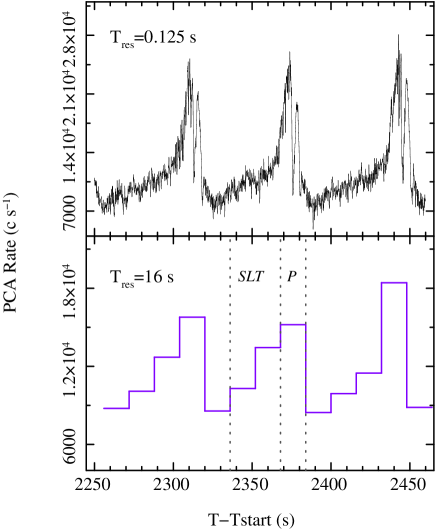
Figure 11: Three bursts as observed by the RXTE/PCA on 2000 October 27 vs time in s from Tstart. The top panel shows the light curve with 0.125 s time resolution and the bottom panel the 16 s one. Spectral data were only available for the 16 s resolution, and the vertical dashed lines in the bottom panel indicate the two selection intervals ($SLT$ and $P$) adopted for the spectral accumulations, as explained in the text.

7 Discussion

The phenomenological model used to fit all spectra, has allowed us to derive some physical information about the characteristics of the source emission in a $\rho$ mode. The scenario that we adopt in the following discussion is that of an accretion disk plus a surrounding high temperature corona. These two components and their strong interaction with each other have been proposed by several authors (Taam et al. 1997; Zdziarski et al. 2001; Done et al. 2004; Ueda et al. 2009) in describing the complex behaviour of GRS 1915+105.

7.1 The multi-temperature disk parameters

The apparent inner radius and temperature are the two most important parameters of the disk component when attempting to interpret the emission of GRS 1915+105 . The values of $kT_{in}$ found in our analysis vary within the range 1 – 2 keV and those of $R_{in}$ are in the range 20–70 km. These results compare quite well with other results for $\rho$ (Vilhu & Nevalainen 1998) and other classes (Belloni et al. 1997), although temperatures as low as 0.7 keV have also been reported (Fender & Belloni 2004).

According to the Shakura-Sunyaev thin disk model, $R_{in}$ depends only on the mass and spin of the black hole. Our results are compatible with the gravitational radius ($R_{g}=GM/c^{2}$) of a 14 $M_{\odot}$ black hole, which is equal to $\sim$21 km. As pointed out by Vierdayanti et al. (2010), to evaluate the $true$ inner radius $R_{in}^{*}$ we must consider the relativistic and spectral hardening corrections, which can be factorized as (Kubota et al. 1998)

$$R_{in}^{*}=\kappa^{2}\zeta R_{in}$$ (1)

adopting their values ($\kappa=1.7$, $\zeta=0.412$), we obtain values larger than $R_{g}$ within the reported uncertainties.

In any case, our lower values of $R_{in}^{*}$ are smaller than the Schwarzschild radius $R_{S}=2R_{g}$. This might be an indication of either a rapidly rotating black hole or a slim accretion disk at about the Eddington luminosity. Indications of a spinning black hole in GRS 1915+105 have been presented by several authors (Middleton et al. 2006, and references therein), who estimated a dimensionless spin parameter $a=Jc/GM^{2}$, where $J$ is the angular momentum of the black hole, equal to about $\sim$0.7. With this value, a minimum distance of $\sim$36 km is acceptable, and considering the large uncertainty in the mass, which might be slightly overestimated, our results are not in conflict with the general scenario adopted for this peculiar source. On the other hand, the calculations of Watarai et al. (2000) for the emission from a slim disk, demonstrated that radiation can be produced at distances much smaller than the last stable orbit, i.e. in the region between $R_{S}$ and $3R_{S}$.

The plot of $T_{in}$ vs $R_{in}$ for the multi-temperature disk obtained for all the fitted spectra is shown in the top panel of Fig. 12. The points of SLT-1 and SLT-2 form two clusters with the same temperature range but clearly separated in terms of $R_{in}$, because of the different flux levels: both clusters exhibit an anticorrelation between the two parameters. The tight correlation is clearly evident between P-1 and P-2, and appears to behave coherently during the entire observation. We fitted the parameter values for these two sets with a single power-law

$$T_{in}=CR^{-q}_{in},$$ (2)

leaving the exponent $q$ as a free parameter and obtained $q=$0.46$\pm$0.01; the fitting relation is shown in Fig. 12 with a solid line. This result translates into an almost constant flux at the peak, as shown in the bottom panel of Fig. 12, where the disk luminosity for all the spectra is plotted vs $kT_{in}$.

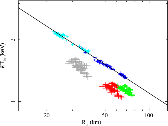
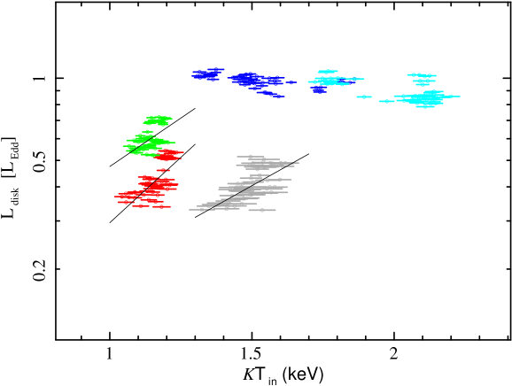
Figure 12: Upper panel: temperature of the multi-color disk vs apparent inner radius. Lower panel: disk luminosity, in units of Eddington luminosity, vs the inner temperature. The continuous black lines are the best-fit models (see text).

Observations of several BHCs have shown that whenever changes have been detected, the luminosity of the disk varies in proportion to $T^{4}$ (Done et al. 2007, and reference within). However, deviations from this relation of the form $L\propto T^{2}$ have been observed in some objects, as in the case of XTE J1550-564, which has an inclination angle of $\sim$70^∘ and a mass 8–11 $M_{\odot}$, and exhibits superluminal jets (Kubota & Done 2004; Kubota & Makishima 2004), similar to GRS 1915+105. Fitting points from all segments, except for that containing the pulse, with a power-law, the resulting values for the temperature exponent are 2.7$\pm$0.4 for SLT-1, 2.0$\pm$0.5 for SLT-2, and 1.9$\pm$0.2 for FDT, respectively. Several models have been proposed to explain the relation $L\propto T^{2}$ for a slim disk where advection dominates the energy transfer in the inner region and reduces the radiation efficiency (Watarai et al. 2000). Moreover, the effects of the large inclination angle cannot be neglected since deviations from the $L\propto T^{4}$ relation are mainly observed in highly inclined sources (Done et al. 2007).

7.2 The corona

The emission of the corona has been detected up to 600 keV without any break and can be interpreted in terms of both a thermal and a non-thermal electron population (Zdziarski et al. 2001). The output spectrum of the thermal component, which is mainly responsible for the spectrum in the BeppoSAX band, depends on the Comptonization parameter $y$, defined as (Rybicki & Lightman 1979)

$$y=4\frac{kT_{el}}{m_{e}c^{2}}{\rm Max}(\tau,\tau^{2}),$$ (3)

where $m_{e}$ is the electron mass and $c$ the speed of light. The values of $y$ vs segment are plotted in Fig. 13; no large variations are observed between the time intervals I and II (continuous and dashed lines), while interval III is characterized by higher values, in agreement with the results for the absolute flux emitted by the corona. Significant variations in $y$ are observed for the segments with higher values in both $SLT$ and $FDT$, while these variations are smaller than 0.1 in the $pulse$, in accordance with the trend in the flux.

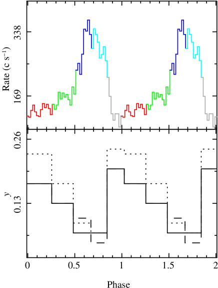
Figure 13: Corona: Variability of the Comptonization parameters $y$ with the burst segments. Interval I is represented with a solid line, II with a dashed line, and III with a dotted line. The top panel shows the MECS rate for comparison; two bursts are shown for clarity.

As shown by Sunyaev & Titarchuk (1980), the ratio of the luminosity of the Comptonizing corona $L_{c}$ to the luminosity of the source of the seed photons ($L_{0}$) for $kT_{e}>h\nu$ is a function of the spectral index, thus for two different segments we have

$$\frac{L_{cj}}{L_{ci}}=\frac{L_{0j}}{L_{0i}}\times f(\Gamma_{j},\Gamma_{i}),$$ (4)

where $i$ and $j$ indicate different segments and $\Gamma$ is the energy index. The spectral index values obtained for the model $v$, are practically constant with $\Gamma\simeq$1.6 (see model $v$ in Appendix A), hence the function $f(\Gamma_{j},\Gamma_{i})$ is close to unity. The decrease in the corona luminosity observed at the peak section could then be attributed to a reduction in the size of the corona itself. Models of disk+corona systems have shown that strong interactions between the two components are able to explain the constant spectral index in term of a tight interaction between the temperature and the optical depth of the corona (Haardt & Maraschi 1991). Moreover, the thermal coupling of the disk and the corona would result in either the evaporation of the disk or the condensation of the corona depending on the accretion rate (Liu et al. 2011; Meyer et al. 2007; Haardt 1993).

8 Summary and conclusion

The spectra of GRS1915+105 that we have accumulated in five segments of the burst of the $\rho$ class have been modeled with several combinations of spectral laws. Only two models were found to provide acceptable fits to all spectra: a multi-color disk with both a black-body and power law, and a disk plus an hybrid corona. Since the former does not have a consistent physical interpretation, we studied the spectral changes in the source based on the basis of the latter.

The following conclusions can be inferred from the analysis of the best-fit values of the parameters:

• The total 0.01-200 keV luminosity of the source in all segments, although the pulse displays a small variation with time in the first 300 ks and sharply increases to a second almost constant level in the last 200 ks. This step-like behaviour is found for most of the spectral parameters, with opposite trends. The luminosity of the pulse remains remarkably stable with time, in the MECS range (1.6-10 keV) despite the variation in the relative best-fit parameters.

• The disk luminosity increases in the pulse and the $R_{in}-T_{in}$ correlation can be more accurately interpreted using the slim disk model.

• The luminosity of the corona is lower at the bursts, possibly because the corona condenses onto the disk.

We stress that some of these results are model-independent being mainly related to the observed rate. All models that we have investigated show that the luminosity below 10 keV reaches the same level in all runs at the peak, whereas at the same time the flux above 20 keV decreases respect to the $SLT$. This behaviour should be taken into account in any more detailed modelings of the complex emission of this source.

Appendix A: Spectral models

We summarize the results obtained with several combinations of spectral functions in XSPEC, which did not provide acceptable results for all segments.

$i$) – Multi-temperature black-body disk + power law: this is one of the simplest models frequently adopted in the spectral analysis of GRS 1915+105 observations (Belloni et al. 1997; Taam et al. 1997). We obtained acceptable reduced $\chi^{2}$ only for a few spectra and, in all data series, large residuals were found to be apparent above 10 keV, which cannot be due to instrumental errors because they were not eliminated by a change in the intercalibration factors within the acceptable range. Adding an exponential cut-off to the power law improves the fits giving narrower reduced $\chi^{2}$ distributions, which are marginally compatible ($\sim$2.5 Gaussian $\sigma$ far) with the expected one for the spectra in the SLT-1, SLT-2, and FDT segments where an average spectral index of 2.4 and a cut-off at 60 keV are measured. However, large residuals above 30 keV in the P-1 and P-2 spectra, caused by the underestimation of the flux, produce distributions of the reduced $\chi^{2}$ of negligible probability of being equivalent to the expected one.

$ii$) – Multi-temperature black-body disk + Comptonised spectrum: the change in the cut-off power law with a comptonization spectrum (Sunyaev & Titarchuk 1980) from high temperature electrons (compst) provides the same results as the previous model.

$iii$) –Multi-temperature black-body disk + power law + reflection from accretion disk: according to previous results (Feroci et al. 1999; Martocchia et al. 2002), we added the Compton reflection from an accretion disk that is either cold (pexrav) or ionized (pexriv) (Magdziarz & Zdziarski 1995) to the multi-temperature black-body disk plus power-law model. These models did not originally include any iron emission line which was added with a Gaussian of fixed width (0.1 keV). Acceptable fits were obtained for the FDT interval, where the spectral statistics are the lowest, and in the SLT-1 spectra before the flux increase at 380 ks; the $\chi^{2}$ distribution in these cases is compatible to within 2$\sigma$ with the expected one. The two models pexriv and pexrav provide compatible best-fit parameters, and in particular the ionization parameter in pexriv assumes values compatible with zero. In the other segments, the model is unable to describe the data above 15 keV, where the highest residuals are observed.

$iv$) – Comptonization from bulk-motion matter: the model (BMC in XSPEC) was developed by Titarchuk et al. (1997) to describe the emission of accreting matter onto a black hole and takes into account the Comptonization of soft photons by a hot gas and the gain in energy originating from the dynamic bulk motion. The combination of two BMC components, which was used by Titarchuk & Seifina (2009) to fit many RXTE spectra of GRS 1915+105, is characterized by the black-body temperature of the soft photon source, a spectral (energy) index, and an illumination parameter related to the fraction of the bulk-motion flow irradiated by the thermal photon source. We left the temperatures of the two BMC as free parameters, because fixing them to the value used by Titarchuk & Seifina (2009) for the RXTE data (1 keV) did not provide acceptable fits to all spectra. An iron line with a Gaussian shape was added to the model, together with an high energy cut-off for one of the two BMC components. Once again, we found that the best-fit spectral distributions, particularly those of the P-1 and P-2 intervals, were not acceptable, in term of either the $\chi^{2}$ values or the large residuals.

The use of an equivalent column density, $N_{H}$ = 5$\times$10²² cm^-2, as the one already considered by Titarchuk & Seifina (2009), provided only a marginal improvement to the fits. The spectra from the SLT-1 and FDT intervals could be modeled by a combination of two BMCs, the $\chi^{2}$ distribution of the spectra were compatible at the 2$\sigma$ level with the expected ones, and the spectral parameters of the first BMC are well-defined with an approximately stable temperature ($kT\simeq$ 1 keV), photon index ($\Gamma$ = 2.8), and Comptonised fraction ($f$ = 0.5). The second BMC has a flux about 60% fainter than the first and a lower temperature ($kT\simeq$ 0.5 keV), but the photon index and the Comptonised fraction are not confined for almost all spectra. Spectra for the SLT-2 intervals are marginally compatible with the model, their distribution $\sim$2.5 Gaussian $\sigma$ being far from that expected, while large residuals above 20–30 keV are present in the pulse spectra (see Fig. 5). Moreover, the $\chi^{2}$ distribution is not compatible with the expected one.

$v$) –Multi-temperature black-body disk + power law + black body: To reduce the large deviations in the residuals between 10 and 30 keV obtained with the other composite phenomenological models, we added to the multi-temperature black-body disk plus power law a third spectral component whose emission is mainly concentrated in this limited band. This model cannot be rejected based on statistical arguments giving acceptable reduced $\chi^{2}$ and flat residuals for all spectra in all segments. The results for the disk are in close agreement with those relative to the “good model”. The power law shows a flux that decreases at the peak coherently with the results of the disk+hybrid corona model and the spectral index displays small variations ($<$10%) with both time and segment, having a mean value of $\alpha$=2.6. The black-body temperature ranges between 3 and 6 keV with the highest values being observed during the $SLT$; its contribution to the source luminosity is always very low, but becomes significant at energies higher than $\sim$ 10 kev, particularly in the pulse, when the power law is faint. No correlation with the power-law luminosity is observed during the bursts, and we note moreover that during these periods it subtends a different spectral range, across which the temperature decreases to 3 keV. However, a consistent scenario to explain the nature and the changes in this component cannot be easily envisaged. Titarchuk & Seifina (2009) also found a similar component with a temperature of 4–5 keV in some of the spectra observed with RXTE and proposed an interpretation in terms of a highly gravitationally redshifted annihilation line. Such a high redshift can be reached only if the emission region is at an extremely short distance from the Schwarzschild radius, and therefore it seems quite unlikely that the flux would exhibit the same modulation of the disk.

References

- Abramowicz et al. (1988) Abramowicz, M. A., Czerny, B., Lasota, J. P., & Szuszkiewicz, E. 1988, ApJ, 332, 646
- Anders & Grevesse (1989) Anders, E. & Grevesse, N. 1989, Geochim. Cosmochim. Acta., 53, 197
- Belloni et al. (2000) Belloni, T., Klein-Wolt, M., Méndez, M., van der Klis, M., & van Paradijs, J. 2000, A&A, 355, 271
- Belloni et al. (1997) Belloni, T., Mendez, M., King, A. R., van der Klis, M., & van Paradijs, J. 1997, ApJ, 488, L109+
- Boella et al. (1997) Boella, G., Chiappetti, L., Conti, G., et al. 1997, A&AS, 122, 327
- Castro-Tirado et al. (1992) Castro-Tirado, A. J., Brandt, S., & Lund, N. 1992, IAUC, 5590, 2
- Chaty et al. (1996) Chaty, S., Mirabel, I. F., Duc, P. A., Wink, J. E., & Rodriguez, L. F. 1996, A&A, 310, 825
- Dickey & Lockman (1990) Dickey, J. M. & Lockman, F. J. 1990, ARA&A, 28, 215
- Done et al. (2007) Done, C., Gierliński, M., & Kubota, A. 2007, A&A Rev., 15, 1
- Done et al. (2004) Done, C., Wardziński, G., & Gierliński, M. 2004, MNRAS, 349, 393
- Fender & Belloni (2004) Fender, R. & Belloni, T. 2004, ARA&A, 42, 317
- Fender et al. (1999) Fender, R. P., Garrington, S. T., McKay, D. J., et al. 1999, MNRAS, 304, 865
- Feroci et al. (1999) Feroci, M., Matt, G., Pooley, G., et al. 1999, A&A, 351, 985
- Frontera et al. (1997) Frontera, F., Costa, E., dal Fiume, D., et al. 1997, A&AS, 122, 357
- Greiner et al. (2001) Greiner, J., Cuby, J. G., & McCaughrean, M. J. 2001, Nature, 414, 522
- Greiner et al. (1996) Greiner, J., Morgan, E. H., & Remillard, R. A. 1996, ApJ, 473, L107+
- Haardt (1993) Haardt, F. 1993, ApJ, 413, 680
- Haardt & Maraschi (1991) Haardt, F. & Maraschi, L. 1991, ApJ, 380, L51
- Hannikainen et al. (2005) Hannikainen, D. C., Rodriguez, J., Vilhu, O., et al. 2005, A&A, 435, 995
- Harlaftis & Greiner (2004) Harlaftis, E. T. & Greiner, J. 2004, A&A, 414, L13
- Klein-Wolt et al. (2002) Klein-Wolt, M., Fender, R. P., Pooley, G. G., et al. 2002, MNRAS, 331, 745
- Kubota & Done (2004) Kubota, A. & Done, C. 2004, MNRAS, 353, 980
- Kubota & Makishima (2004) Kubota, A. & Makishima, K. 2004, ApJ, 601, 428
- Kubota et al. (1998) Kubota, A., Tanaka, Y., Makishima, K., et al. 1998, PASJ, 50, 667
- Lee et al. (2002) Lee, J. C., Reynolds, C. S., Remillard, R., et al. 2002, ApJ, 567, 1102
- Liu et al. (2011) Liu, B. F., Done, C., & Taam, R. E. 2011, ApJ, 726, 10
- Magdziarz & Zdziarski (1995) Magdziarz, P. & Zdziarski, A. A. 1995, MNRAS, 273, 837
- Manzo et al. (1997) Manzo, G., Giarrusso, S., Santangelo, A., et al. 1997, A&AS, 122, 341
- Martocchia et al. (2006) Martocchia, A., Matt, G., Belloni, T., et al. 2006, A&A, 448, 677
- Martocchia et al. (2002) Martocchia, A., Matt, G., Karas, V., Belloni, T., & Feroci, M. 2002, A&A, 387, 215
- Massaro et al. (2010) Massaro, E., Ventura, G., Massa, F., et al. 2010, A&A, 513, A21+
- Meyer et al. (2007) Meyer, F., Liu, B. F., & Meyer-Hofmeister, E. 2007, A&A, 463, 1
- Middleton et al. (2006) Middleton, M., Done, C., Gierliński, M., & Davis, S. W. 2006, MNRAS, 373, 1004
- Mirabel & Rodríguez (1994) Mirabel, I. F. & Rodríguez, L. F. 1994, Nature, 371, 46
- Mitsuda et al. (1984) Mitsuda, K., Inoue, H., Koyama, K., et al. 1984, PASJ, 36, 741
- Neilsen et al. (2011) Neilsen, J., Remillard, R. A., & Lee, J. C. 2011, ApJ, 737, 69
- Poutanen & Svensson (1996) Poutanen, J. & Svensson, R. 1996, ApJ, 470, 249
- Rodriguez et al. (2008) Rodriguez, J., Shaw, S. E., Hannikainen, D. C., et al. 2008, ApJ, 675, 1449
- Rybicki & Lightman (1979) Rybicki, G. B. & Lightman, A. P. 1979, Radiative processes in astrophysics, ed. Rybicki, G. B. & Lightman, A. P.
- Smith et al. (2002) Smith, R. K., Edgar, R. J., & Shafer, R. A. 2002, ApJ, 581, 562
- Sobolewska & Życki (2003) Sobolewska, M. A. & Życki, P. T. 2003, A&A, 400, 553
- Sunyaev & Titarchuk (1980) Sunyaev, R. A. & Titarchuk, L. G. 1980, A&A, 86, 121
- Taam et al. (1997) Taam, R. E., Chen, X., & Swank, J. H. 1997, ApJ, 485, L83+
- Titarchuk et al. (1997) Titarchuk, L., Mastichiadis, A., & Kylafis, N. D. 1997, ApJ, 487, 834
- Titarchuk & Seifina (2009) Titarchuk, L. & Seifina, E. 2009, ApJ, 706, 1463
- Trudolyubov (2001) Trudolyubov, S. P. 2001, ApJ, 558, 276
- Ueda et al. (2010) Ueda, Y., Honda, K., Takahashi, H., et al. 2010, ApJ, 713, 257
- Ueda et al. (2009) Ueda, Y., Yamaoka, K., & Remillard, R. 2009, ApJ, 695, 888
- van Oers et al. (2010) van Oers, P., Markoff, S., Rahoui, F., et al. 2010, MNRAS, 409, 763
- Vierdayanti et al. (2010) Vierdayanti, K., Mineshige, S., & Ueda, Y. 2010, PASJ, 62, 239
- Vilhu & Nevalainen (1998) Vilhu, O. & Nevalainen, J. 1998, ApJ, 508, L85
- Watarai et al. (2000) Watarai, K., Fukue, J., Takeuchi, M., & Mineshige, S. 2000, PASJ, 52, 133
- Yadav (2006) Yadav, J. S. 2006, ApJ, 646, 385
- Yadav et al. (1999) Yadav, J. S., Rao, A. R., Agrawal, P. C., et al. 1999, ApJ, 517, 935
- Zdziarski et al. (2005) Zdziarski, A. A., Gierliński, M., Rao, A. R., Vadawale, S. V., & Mikołajewska, J. 2005, MNRAS, 360, 825
- Zdziarski et al. (2001) Zdziarski, A. A., Grove, J. E., Poutanen, J., Rao, A. R., & Vadawale, S. V. 2001, ApJ, 554, L45