Annihilation of vortex dipoles in an Oblate Bose-Einstein Condensate

Abstract

We theoretically explore the annihilation of vortex dipoles, generated when an obstacle moves through an oblate Bose-Einstein condensate, and examine the energetics of the annihilation event. We show that the gray soliton, which results from the vortex dipole annihilation, is lower in energy than the vortex dipole. We also investigate the annihilation events numerically and observe that the annihilation occurs only when the vortex dipole overtakes the obstacle and comes closer than the coherence length. Furthermore, we find that the noise reduces the probability of annihilation events. This may explain the lack of annihilation events in experimental realizations.

I Introduction

One of the important developments in recent experiments on atomic Bose-Einstein condensates (BECs) is the creation of vortices and the study of their dynamics Anglin2002 ; PRL.83.2498 . Equally important is the recent experimental observation of a vortex dipole, which consists of a vortex-antivortex pair, when an obstacle moves through a BEC PRL.104.160401 and observation of vortex dipoles produced through phase imprinting F03092010 ; PRA.64.043601 . In superfluids, the vortices carry quantized angular momenta and are the topological defects, which often serve as the conclusive evidence of superfluidity. In a vortex dipole, vortices of opposite circulation cancel each other’s angular momentum and thus carry only linear momentum. This is the cause of several exotic phenomena like leap frogging, snake instability PRA.65.043612 , orbital motion PRA.84 , trapping PRX.1 , and others. The effects of vortices are widespread in classical fluid flow CJ:392656 and optical manipulation Grier2003 . A good description of vortices in superfluids is given in Ref. pethick and review articles rmp.81.647 ; rmp.59.87 . More detailed discussion of vortices is given in Ref. okulov .

Among the important phenomena associated with the Bose-Einstein condensate (BEC), the creation, dynamics, and annihilation of vortex dipoles carry useful information associated with the system. Several methods have been suggested to nucleate vortices and recently, nucleation of the vortices have been observed experimentally by passing a Gaussian obstacle through the BEC with a speed greater than some critical speed PRL.104.160401 . The trajectories of these vortex dipoles are ring-structured as described in Refs. PRA.61.013604 ; PRA.77.053610 . The annihilation of vortices in the BEC has been mentioned in a number of theoretical studies JLTP.146.31 ; PRA.84.023637 ; PRB.84.020506 . However, there is a lack of extensive study on this topic. Moreover, the questions related to thermodynamic stability, resulting state after annihilation and its dynamics has not been examined. The study of vortex dipole annihilation will shed light on the process that leads to minimum separation between vortex-antivortex and conditions for annihilation along with other phenomena arising from the dynamics of vortex dipoles.

In this work, we present analytical as well as numerical results related to vortex dipole annihilation for an oblate BEC at zero temperature. The results are obtained using Gross-Pitaevskii (GP) equation. In Section II of this article, we provide a brief description of the two-dimensional (2D) GP equation and vortex dipole solutions. Condensate with diametric vortex dipole and gray soltion are studied and this is described in section III. Section III contains studies done in the strong as well as weak interacting systems. Annihilation of vortex dipoles is analysed from the energies obtained from the analytical calculations. The numerical results, confirming the analytic results, are discussed in Section IV, and we then conclude.

II Superfluid vortex dipole and its generation

In the mean-field approximation, the dynamics of a dilute BEC is very well described by the GP equation

$$i\hbar\partial_{t}\Psi(\textbf{r},t)=[{\cal H}+U|\Psi(\textbf{r},t)|^{2}]\Psi(\textbf{r},t),$$ (1)

where ${\cal H}$, $U$ and $\Psi$ are the single-particle Hamiltonian, interaction strength and order parameter of the condensate respectively. The order parameter, $\Psi$, is normalized to $N$, the total number of atoms in the condensate. In the present case, the single-particle Hamiltonian ${\cal H}$ consists of the kinetic-energy operator, an axis-symmetric harmonic trapping potential, and a gaussian obstacle potential, that is,

$${\cal H}=-\frac{\hbar^{2}}{2m}\nabla^{2}+\frac{m\omega^{2}}{2}(x^{2}+\alpha^{2}y^{2}+\beta^{2}z^{2})+V_{\rm obs}(x,y,t),$$ (2)

where $\alpha$ and $\beta$ are the anisotropies along $y$ and $z$ axis respectively, and $V_{\rm obs}(x,y,t)$ is the repulsive Gaussian obstacle potential. Experimentally, a blue-detuned laser beam is used to generate the $V_{\rm obs}(x,y,t)$ and it can be written as

$$V_{\rm obs}(x,y,t)=V_{0}(t)\exp\left[-2\frac{(x-vt)^{2}+y^{2}}{w_{0}^{2}}\right],$$ (3)

where $V_{0}(t)$ is the potential at the center of the Gaussian obstacle at time $t$, $v$ is the velocity of the obstacle along $x$-axis, and $w_{0}$ is the radius of repulsive obstacle potential. In the present work, we consider the motion of obstacle along $x$-axis only. Defining the oscillator length of the trapping potential as $a_{\rm osc}=\sqrt{\hbar/(m\omega)}$, and considering $\hbar\omega$ as the unit of energy, we can then rewrite the equations in dimensionless form with transformations $\tilde{\mathbf{r}}=\mathbf{r}/a_{\rm osc}$, $\tilde{t}=t\omega$, and the transformed order parameter assumes the form

$$\phi(\tilde{\mathbf{r}},\tilde{t})=\sqrt{\frac{a_{\rm osc}^{3}}{N}}\Psi(\mathbf{r},t).$$ (4)

For the sake of notational simplicity, hereafter we denote the scaled quantities without tilde in the rest of the manuscript. In a pancake-shaped trap $\alpha=1$ and $\beta\gg 1$ and the order parameter can then be written as

$$\phi(\mathbf{r},t)=\psi(x,y,t)\zeta(z)\exp(-i\beta t/2),$$ (5)

where $\zeta(z)=(\beta/(2\pi))^{1/4}\exp(-\beta z^{2}/4)$. The Eq. (1) is then reduced to the two dimensional form

$$\left[-\frac{1}{2}\left(\frac{\partial^{2}}{\partial x^{2}}+\frac{\partial^{2}}{\partial y^{2}}\right)+\frac{x^{2}+y^{2}}{2}+\frac{V_{\rm obs}(x,y,t)}{\hbar\omega}\right.$$

$$\left.+u|\psi({\mathbf{r}},t)|^{2}-i\frac{\partial}{\partial t}\right]\psi({\mathbf{r}},t)=0,$$ (6)

where $u=2aN\sqrt{2\pi\beta}/a_{\rm osc}$, with $a$ as the $s$-wave scattering length, is the modified interaction strength. In the present work, we consider condensate consisting of ⁸⁷Rb atoms in $F=1$, $m_{F}=-1$ state with $s=99a_{0}$ prl88 . We have neglected a constant term corresponding to the energy along axial direction as it only shifts the energies and chemical potentials by a constant without affecting the dynamics. We solve this equation numerically using the Crank-Nicholson method Muruganandam20091888 .

There are several theoretical and experimental proposals to generate vortices in non-rotating traps. These include stirring of the condensate using blue-detuned laser or several laser beams PRL.104.160401 ; PRA.61.013604 , adiabatic passage PRL.80.2972 , Raman transitions in binary condensate systems PRL.79.4728 , laser beam vortex guiding s003400000337 , and phase imprinting PRA.64.043601 . Among these methods, the easiest one to nucleate vortex dipoles is by stirring a BEC with a blue-detuned laser beam. When the velocity of the laser beam exceeds a critical velocity, vortex-antivortex pairs are released from the localized dip in the number density created due to the laser beam. These vortex dipoles then move through the BEC and exhibit various interesting dynamics F03092010 ; PRA.61.013604 ; PRA.83.011603 . The critical velocity depends on the number density, width and intensity of the laser beam, and the frequency of the trapping potential. This nucleation process exhibits a high degree of coherence and stability, allowing us to map out the annihilation of the dipoles. In an axis-symmetric trap, a vortex dipole is a metastable state of superfluid flow with long lifetime.

III Condensates with vortex dipole or gray soliton

To analyse the vortex dipole annihilation, we consider a model system where the vortex-antivortex dipole pair and gray soliton, which may be generated when annihilation of vortex dipole occures, are static. However, we vary the distance of separation and examine the energy of the total system. The present system can be studied under two regims: strongly interactly system, and weakly interacting system. The strongly interacting system is studied considering $\phi$ with Thomas-Fermi (TF) approximation and the weakly interacting system is studied considering the Gaussian form of $\phi$.

III.1 Strongly interacting system with TF approximation

For the $Na/a_{\rm osc}\gg 1$ case, we use TF approximation to determine the steady state density profile and energy of the condensate. To begin with, we consider a condensate with vortex dipole and later, with gray soliton.

III.1.1 Diametric vortex dipole

We consider a condensate consisting of $N$ atoms in a purely harmonic potential

$$V(x,y)=\frac{x^{2}+y^{2}}{2}.$$ (7)

Consider that the condensate has a vortex dipole, consisting of a vortex and an antivortex located at $(0,v_{2})$ and $(0,-v_{2})$, respectively. The cores of the vortex and antivortes can be approximated as cicular regions centered around $(0,v_{2})$ and $(0,-v_{2})$ and with radii equal to the coherence lenght $\xi$. At the cores, we consider the density to be equal to zero. Hence, we use the TF approximation and adopt the following piecewise ansatz for the density of the condensate

$$n(x,y) = \left\{\begin{aligned} &0\!&&\text{ for }x^{2}+y^{2}>R^{2}\\ &0\!&&\text{ for }[x^{2}+(y\pm v_{2})^{2}]\leqslant\xi^{2}\\ &\left[\frac{\mu-V(x,y)}{u}\right]&&\text{ for }\left\{\begin{aligned} &x^{2}+y^{2}\leqslant R^{2}~{}\&\\ &~{}[x^{2}+(y\pm v_{2})^{2}]>\xi^{2},\end{aligned}\right.\end{aligned}\right.$$ (8)

where $R=\sqrt{2\mu}$ is the spatial extent of the condensate in TF approximation, and $\xi=1/R$ is the coherence length at the center of the trap. Normalizing this ansatz yields

$$\frac{\pi\left(2-4R^{4}+R^{8}+4R^{2}v_{2}^{2}\right)}{4R^{4}u}=1.$$ (9)

This equation defines the radius of the condensate. The TF ansatz can be used to calculate the total potential energy arising from the regions outside the cores of the vortices and is given as

$$E_{0}=\frac{\pi\left[1-3R^{8}+R^{12}+3R^{2}v_{2}^{2}\left(2+R^{2}v_{2}^{2}\right)\right]}{12R^{6}u}.$$ (10)

The main energy contribution from the vortex dipole is the kinetic energy due the velocity field associated with it. This energy can be approximated as Zhou

$$E_{\rm KE}=\frac{R^{2}}{u}\text{Log}\left(\frac{2v_{2}}{\xi}\right).$$ (11)

This relation is valid when $\xi\ll v_{2}\ll R$ and in the present work, $\xi\sim 0.06$, $R=15.5~{}a_{\rm osc}$. In order to estimate the energy contributions from the cores of the vortices we approximate the density within the cores as

$$n(x,y)=\left\{\begin{aligned} \frac{2n_{0}[x^{2}+(y-v_{2})^{2}]}{x^{2}+(y-v_{2})^{2}+\xi^{2}}&\text{ for }[x^{2}+(y-v_{2})^{2}]<\xi^{2}\\ \frac{2n_{0}[x^{2}+(y+v_{2})^{2}]}{x^{2}+(y+v_{2})^{2}+\xi^{2}}&\text{ for }[x^{2}+(y+v_{2})^{2}]<\xi^{2},\end{aligned}\right.$$ (12)

where $n_{0}$ is the average TF density on the circle $x^{2}+(y\pm v_{2})^{2}=\xi^{2}$. Assuming that the normalization is still defined by equation Eq. (9), Eq. (12) can be used to calculate energy contribution from the core region. The energy within the consist of

$$E^{\rm q}_{\rm c} = \frac{6\pi n_{0}}{8},$$ (13)

$$E^{\rm tr}_{\rm c} = \pi\xi^{4}(\text{Log}[4]-1)n_{0},$$ (14)

$$E^{\rm int}_{\rm c} = 2\pi u\xi^{2}(3-\text{Log}[16])n_{0}^{2},$$ (15)

where, $E^{\rm q}_{\rm c}$, $E^{\rm tr}_{\rm c}$ and $E^{\rm int}_{\rm c}$ are the energies arising from the quantum pressure, trapping potential and interaction within the core region, respectively. Thus, the total energy of the condensate with a vortex dipole is

$$E_{\rm vd}=E_{0}+E_{\rm KE}+E^{\rm q}_{\rm c}+E^{\rm tr}_{\rm c}+E^{\rm int}_{\rm c}.$$ (16)

The variation of $E_{\rm vd}$ as a function of $v_{2}$ is plotted in Fig. 1.

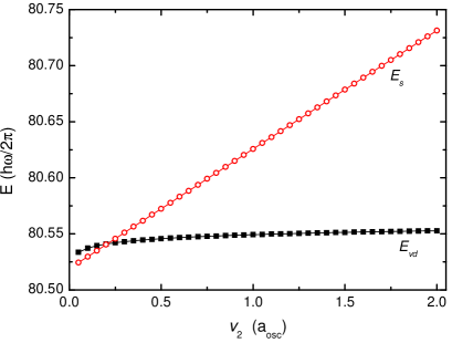
Figure 1: Comparing the energy of vortex dipole and band soliton under TF approximations. The crossover in energy can be seen through ansartz choosen and the analytical expressions obtained.

III.1.2 Gray soliton

For gray soliton extending from (0, $-v_{2}$) to (0, $v_{2}$) along $y$-axis, we use the following piecewise ansatz in the TF approximation

$$n(x,y)=\left\{\begin{aligned} &0&&\text{ for }x^{2}+y^{2}>R^{2},\\ &\left[\frac{\mu-V(x,y)}{u}\right]&&\text{ for }\left\{\begin{aligned} x^{2}+y^{2}\leq R^{2},\\ |x|>\xi,\\ |y|>v_{2},\end{aligned}\right.\\ &\left[\frac{\mu-V(x,y)}{u}\right]\frac{2x^{2}}{x^{2}+\xi^{2}}&&\text{ for }|x|\leq\xi~{}\&~{}|y|\leq v_{2}.\end{aligned}\right.$$ (17)

And, the normalization condition leads to following constraint on the radius of the condensate

$$\frac{1}{12R^{3}u} \left[3\pi R^{7}+4v_{2}\left(10+6R^{4}-3\pi\left(1+R^{4}\right)\right.\right.$$ (18)

$$+\left.\left.(-2+\pi)R^{2}v_{2}^{2}\right)\right]=1.$$

For the gray soliton, other than the quantum pressure, there is no need to separate out the energy associated with the trapping and interaction potential within the soliton. So, the total energy of the system is

$$E_{\rm s}=E_{0}+E^{\rm q}_{\rm c},$$ (19)

where, $E_{0}$ is the potential energy associated with the system and $E^{\rm q}_{\rm c}$ is the energy arising from the quantum pressure. These are given as

$$E_{0} = \int\int\left[V(x,y)n(x,y)+\frac{u}{2}n(x,y)^{2}\right]\mathrm{d}x\mathrm{d}y,$$

$$E^{\rm q}_{\rm c} = \frac{1}{2}\int_{-\xi}^{\xi}\left[\int_{-v_{2}}^{v_{2}}|\nabla_{xy}\sqrt{n(x,y)}|^{2}\mathrm{d}y\right]\mathrm{d}x.$$ (20)

From the expression of the $n(x,y)$ in Eq. (17), we get

$$E_{0} = \frac{1}{180R^{5}u}\left\{15\pi R^{11}+3\left[236-75\pi\right.\right.$$ (21)

$$\left.+20(19-6\pi)R^{4}+15(8-3\pi)R^{8}\right]v_{2}$$

$$\left.+10R^{2}\left[-28+9\pi+6(-3+\pi)R^{4}\right]v_{2}^{3}\right.$$

$$\left.-9(-4+\pi)R^{4}v_{2}^{5}\right\}$$

$$E^{\rm q}_{\rm c} = -\frac{(8+3\pi)v_{2}\left(-3R^{2}+3\xi^{2}+v_{2}^{2}\right)}{48u\xi}.$$ (22)

Interestingly, the $E^{\rm q}_{\rm c}$ has a $1/\xi$ dependence, which is to be expected as smaller $\xi$ implies larger density variation and translates to higher quantum pressure.

For illustration, the vortex dipole and gray soliton inside the condensate is shown in Fig. 2. The vortex dipole is located at ($1$, 0) and ($-1$, 0) while the gray soliton extends from ($-1$, 0) to ($1$, 0) along the $x$-axis. In the case of vortex dipoles, the phase varies from 0 to $2\pi$, if one goes around the point of singularity. While in the case of gray soliton, there is a phase discontinuity of $\pi$ along the line forming the soliton. The number density at the point of singularities are zero.

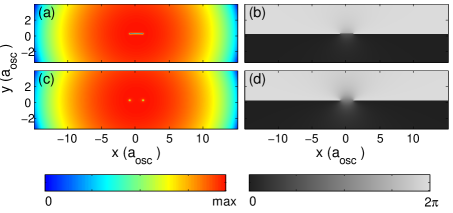
Figure 2: Band soliton (top) and vortex dipole (bottom) with density profile (left) and phase profile (right) obtained numerically.

In Fig. 1, $E_{s}$ is plotted as a function of $v_{2}$ and the values varies from 0.05 $a_{\rm osc}$ to 2.0 $a_{\rm osc}$. From the figure it is evident that for $v_{2}\leqslant 0.2$, the value of $E_{\rm vd}$ is higher than $E_{\rm s}$ and hence, the gray soliton is the energetically favoured state of the system. However, when $v_{2}>0.2$ the vortex dipole state is the energetically favorable. This analytical result is a compelling reason to study the annihilation of vortex dipoles and formation of gray solitons.

III.2 Weakly interacting system with gaussian approximation

In $Na/a_{\rm osc}\ll 1$ regime, a simplistic model of a vortex dipoles in the BEC of trapped dilute atomic gases can be considered as the superposition of harmonic oscillator eigenstates. The minimalist wave function which supports a vortex and antivortex at cordinates $(-a/c,-\sqrt{b/d})$ and $(-a/c,\sqrt{b/d})$ is

$$\psi(x,y)=e^{-i\mu t}\left(ia-b+ixc+dy^{2}\right)e^{-(x^{2}+y^{2})/f},$$ (23)

where $a$, $b$, $c$, $d$, and $f$ are positive variational parameters and $\mu$ is the chemical potential of the system. The wave function is a superposition of the scaled ground state and the first and the second excited states of harmonic oscillator along the $x$ and $y$-axes, respectively. The wave function is ideal for weakly interacting condensates.

Consider that the vortex and antivortex are located on the diameter of the condensate. Without loss of generality, we consider the diameter as coinciding with the $y$-axis, which is equivalent to $a=0$ in Eq. 23. Such an assumption does not modify the qualitative descriptions, but expressions are far less complicated. The wave function is then

$$\psi(x,y,t)=e^{-i\mu t}\left[-b+icx+dy^{2}\right]e^{-(x^{2}+y^{2})/f}.$$ (24)

The nontrivial phase of the wave function $\theta$ is discontinuous along $x=0$ line for $-\sqrt{b/d}\leqslant y\leqslant\sqrt{b/d}$. Across the discontinuity, there is a phase change from $-\pi$ to $\pi$ as we traverse along $x$-axis from $0^{-}$ to $0^{+}$ and this phase variation is shown in Fig. 3. So, there is a discontinuity across the $y$-axis and this is the typical phase pattern associated with vortex dipoles. For the present case, the ground state wave function is

$$\psi_{\rm g}(x,y,t)=-be^{-i\mu t}e^{-(x^{2}+y^{2})/f},$$ (25)

and from the normalization condition $\int_{-\infty}^{\infty}\int_{-\infty}^{\infty}|\psi_{\rm g}|^{2}\mathrm{d}x\mathrm{d}y=1$, we get the constraint equation

$$b^{2}=\frac{2}{f\pi}.$$ (26)

For general considerations, rewrite the additional term as

$$\delta\psi(x,y,t)=e^{-i\mu t}\left(icx+dy^{2}\right)e^{-(x^{2}+y^{2})/f}.$$ (27)

So that the total wave function $\psi=\psi_{\rm g}+\delta\psi$, where $\delta\psi$ represents an elementary excitation of the condensate. We can calculate the total energy of the system, without the obstacle potential, as

$$E_{\rm vd} = \int_{-\infty}^{\infty}\int_{\infty}^{\infty}\bigg{[}\frac{1}{2}|\nabla_{\perp}\psi(x,y)|^{2}+\frac{x^{2}+y^{2}}{2}|\psi(x,y)|^{2}$$ (28)

$$+u|\psi(x,y)|^{4}\bigg{]}\mathrm{d}x\mathrm{d}y.$$

This is the energy of the condensate with a vortex dipole with the assumption that it is a weakly interacting system. Energy without the vortex may be calculated trivially pethick . In general, the energy added to the system due to the vortex dipole is not large compared to the total and for obvious reason, the angular momentum of the condensate is still zero.

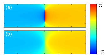
Figure 3: Phase pattern resulting due to a vortex-dipole (a) and gray-soliton (b).

A slight modification to the wave function can describe a solitonic solution along $y$-axis. The form of the modifed wave function is

$$\psi(x,y)=\left[b+icx+dy^{2}\right]e^{-(x^{2}+y^{2})/f},$$ (29)

where except for the change in the sign of $b$, all the terms remain unaltered as in Eq. (23). It is a gray soliton as the density $n\propto(b+dy^{2})^{2}+(a+cx)^{2}$ has a dip but is different from zero. The phase varies smoothly from $-\pi/2$ to $\pi/2$ along the normal to the line which connects $(0,-\sqrt{b/d})$ and $(0,\sqrt{b/d})$. This phase variation is shown in Fig. 3(b).

Using the wave function in Eq. (29), we can then evaluate the total energy of the system $E_{\rm gs}$ and calculate the energy difference between two possible states of the system

$$\Delta E=E_{\rm vd}-E_{\rm gs},$$ (30)

which after evaluation is

$$\Delta E=\frac{bdf^{2}\pi}{256}\left[64b^{2}u+15d^{2}f^{2}u+8f(8+c^{2}u)\right].$$ (31)

The most general solution is when all the constants are positive, then $\Delta E>0$ and the gray soliton is lower in energy. This shows that when the vortex-antivortex collides, it is energetically favourable for them to decay into gray soliton. As discussed in the results section, this is confirmed in the numerical calculations.

The analysis so far is for an ideal system at zero temperature, where we have neglected the thermal fluctuations and perturbations from imperfections. In addition, there is dissipation from three body collision losses in the condensates of dilute atomic gases.

IV Numerical Results

For the numerical computation,w e choose ⁸⁷Rb with $N=2\times 10^{6}$ atoms. The trapping potential and obstacle laser potential parameters are similar as those considered in Ref. PRL.104.160401 , i.e., $\omega/(2\pi)=8$ Hz, $\beta=11.25$, $V_{0}(0)=93.0~{}\hbar\omega$ and $w_{0}=10~{}\mu$m. To nucleate the vortices on the edges of the condensate, the obstacle potential $V_{\rm obs}$ is initially located at $-12.5~{}a_{\rm osc}$ and moves along the $x$ direction at a constant velocity with decreasing intensity until $V_{\rm obs}$ vanishes at $5.18~{}a_{\rm osc}$.

IV.1 Vortex dipole nucleation

We study the nucleation of vortices by $V_{\rm obs}$ with the translation speed $v$ ranging from $80~{}\mu$m/s to $200~{}\mu$m/s. Vortices are not nucleated when the speed is $80~{}\mu$m/s. However, a vortex-antivortex or a vortex dipole is nucleated when the speed is in the range $90~{}\mu$m/s $<v<140~{}\mu$m/s. Increasing the speed of obstacle generates two pairs of vortex dipoles when $140~{}\mu$m/s $\leqslant v<160~{}\mu$m/s and more than two when $v\geqslant 160~{}\mu$m/s. In other words, the number of vortex dipoles created can be controlled with the speed of the obstacle. Creation of vortex dipoles above a critical speed $v_{c}$ is natural as the vortex nucleation must satisfy the Landau criterion Lifshitz . The density and phase of the condensate after the nucleation of vortex dipole for $v=120~{}\mu$m/s is shown in Fig. 4. The figure clearly shows nucleation dynamics of the vortex dipoles.

From numerical calculations, we have determined $v_{c}\approx 90~{}\mu$m/s. This is, however, less than the local acoustic velocity of the medium $s=\sqrt{nU/m}$, which depends on the local condensate density. This also explains the reason for the predominant vortex dipole nucleation around the edge of the condensate where $n$ is lower and $s$ is accordingly lower.

IV.2 Vortex dipole annihilation

It is observed that the vortex dipole annihilation is critically dependent on the initial conditions of the nucleation. For this reason, the annihilation events are observed only for specific range of $v$. As an example, the annihilation event when $v$ is $120~{}\mu$m/s is shown in Fig. 4. In Fig. 4, we can notice the density minima arising from the annihilation and propagating away from the obstacle potential.

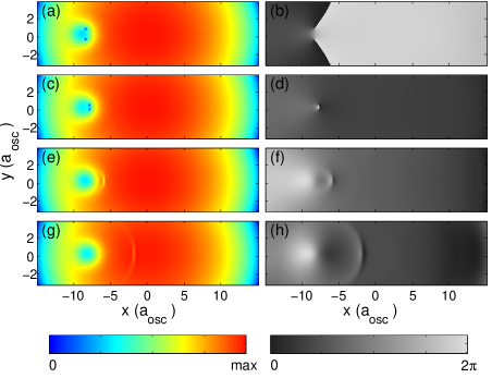
Figure 4: A vortex dipole is nucleated when the obstacle potential traverses the condensate at a speed of $120~{}\mu$m/s. The vortex dipole, however, passes through and overtakes the obstacle. Later, as seen in (e), the vortex dipole annihilates and generates a gray soliton. The figures in the left panel show the density distribution and those on the right show the phase pattern of the condensate. From top to bottom, $t$ = 2.9, 3.1, 3.3, and 3.5 respectively.

A reliable and qualitative way to describe occurrence of annihilation could be achieved by observing the density at the cores of vortex and antivortex which form the dipole. For the vortex, the matter density at the core when $v$ is $120~{}\mu$m/s is shown in Fig 5. In the plot, at time $\approx 3.1868$ (scaled unit), the core density starts increasing. This is because the core starts to fill in with the atoms from around the vortex after the annihilation. This filling process may not complete till it reaches the edge of the condensate and gets reflected inside the condensate.

Figure 5: Density variation at the core of the vortex with time. After the vortex dipole annihilation, density increases till it reaches the bulk value. The values correspond to the obstacle speed of $120~{}\mu$m/s. After annihilation, the number density has been considered from the location of minimum density. X-axis denotes the time elapsed from the starting of obstacle at $-12.5a_{\rm osc}$.

After the annihilation of vortex-antivortex dipole pair, a gray soliton gets generated. We can clearly observe the propagation of this soliton in Fig. 6. The speed of propagation is 1999.6495 $\mu$m/s which is similar to the speed of sound in condensate. During the propagation, the number density on the location of the soliton increases which is clearly visible from Fig. 6 as well as from Fig. 5. To estimate the energy of gray soliton, we have obtained the stationary state with the same positon of vortex dipoles and obstacle potential. The energy difference between stationary state and dynamic state will provide us with the energy of gray soliton as discussed in ref adams . The energy released due to the annihilation is 0.003995 $\hbar\omega$ and is similar to the energy difference observed in Fig. 1, obtained from the TF approximation. We have also observed that this soliton gets reflected back-and-forth from the edge of the condensate. This reflection is similar to the reflection of any pulse from the circular edges.

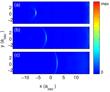
Figure 6: The propagation of the gray soliton after the annihilation of vortex dipole. The higher the value, higher the number density dip at that point. From (a)-(c), $t$ = 3.2, 3.4 and 3.6 respectively.

As discussed in Section. III, annihilation can occur only when it is energetically favorable. In other words, the state with the gray soliton must have lower energy than the vortex dipole. This is clearly seen in the change of total energy of the system, which is shown in Fig. 7. After the annihilation, the energy of the system decreases and continues to do so at a steady rate. Although not shown in the plot, before the annihilation the energy is on an average constant.

Figure 7: Variation in the energy of the system with time (in scaled units). There is a decrease in energy after the vortex dipole annihilation, and the plot is based on the results of calculations in which a vortex dipole is imprinted at ($-2.0~{}a_{\rm osc}$, $\pm 0.1~{}a_{\rm osc}$). It is then allowed to annihilate and evolve in time.

It is to be mentioned that for the parameters considered in the present work, the speed of sound is $2190~{}\mu$m/s and the coherence length of the system is $\sim 0.229~{}\mu$m. These are in agreement with the minimum separation between the vortex and antivortex observed in the analytical work. The energy gap for vortex dipole and gray soliton for the same size matches with the estimates from the ansatz based on TF approximation. The vortex dipole annihilation is not only observed for $V_{\rm obs}=120~{}\mu$m/s, it also occures for other obstacle velocities as well. Once such case, for $V_{\rm obs}=160~{}\mu$m/s, is shown in Fig. 8. In this case, the difference in energy of vortex dipole and gray soliton is 0.002481 $\hbar\omega$.

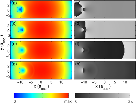
Figure 8: A vortex dipole is nucleated as the obstacle potential traverses the BEC with a speed of $160~{}\mu$m/s. The figures in the left panel shows the density with time, where time progresses from top to bottom. Figures on the right panel show the phase pattern of the condensate. From top to bottom, $t$ = 1.6, 1.8, 2.0, and 4.2 respectively.

One observation, which is common to all the vortex dipoles getting annihilated is the nature of their trajectories. All of them traverse through $V_{\rm obs}$, whereas the ones which do not get annihilated avoid $V_{\rm obs}$. The vortex dipoles are generally nucleated at the aft region of the $V_{\rm obs}$ where there is a trailling superflow. When nucleated very close to each other and with high velocity, the mutual force further increases the velocity of the vortex dipoles. At the same time, it decreases the distance separating vortex and antivortex. So, the kinetic energy is high enough to surpass $V_{\rm obs}$. Later, at some point vortex and antivortex separation is less than $\xi$, and they annihilate.

IV.3 Effect of noise and dissipation

In the numerical studies, the annihilation events are not rare. But, this is in contradiction with the experimental results of Neely and collaborators PRL.104.160401 , they observed no signatures of annihilation events. One possible reason is that our numerical calculations are too ideal, and one immediate remedy is to include fluctuations. For this we introduce white noise during the real time evolution. One immediate outcome is, the symmetry in the trajectory of the vortex and antivortex is lost. The superflow around the vortex is no longer a mirror reflection of the antivortex, which was nearly the case without the white noise. The deviations are shown for an example case in the Fig. 9, where $V_{\rm obs}=180~{}\mu$m/sec. The change in path leads to the suppression of annihilation of vortex dipoles.

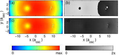
Figure 9: The trajectory of a vortex dipole in the presence of white noise. There is a lack of symmetry in the trajectory of the vortex and antivortex. This reduces the possibility of an annihilation event significantly. The figures in the left (right) panel show the density (phase) of the condensate and time increases from top to bottom figures of each panel. The speed of the obstacle is $180~{}\mu$m/s, and the white noise is at the level of 0.01%. Top and bottom correspond to $t=$ 4.1 and 4.2 respectively from the starting of obstacle at $x=-12.5a_{\rm osc}$.

The other important effect is the loss of atoms from the trap. We have examined the effect of loss terms, which arise from inelastic collisions in the condensate. There are two types of inelastic collisions that lead to the loss of atoms from the trap: two body inelastic collision loss and the three body loss. To model the effect of loss of atoms from the trap, we add the loss terms

$$\frac{-i\hbar}{2}\left[K_{2}|\Psi(\mathbf{r},t)|^{2}+K_{3}|\Psi(\mathbf{r},t)|^{4}\right],$$ (32)

to the Hamiltonian ${\cal H}$. Based on the previous work PRL.80.2097 for ⁸⁷Rb, the inelastic two-body loss rate coefficient $K_{2}=4.5\times 10^{-17}~{}{\rm cm}^{3}~{}{\rm s}^{-1}$, and inelastic three-body loss rate coefficient $K_{3}=3.8\times 10^{-29}~{}{\rm cm}^{6}~{}{\rm s}^{-1}$. With trap loss, the annihilation events continue to occur. However, during the destructive time of flight observations in the experiments, the decreased atom numbers may lower the contrast and reduce the possibility of observing an annihilation event.

V Conclusions

When an obstacle moves through a condensate above a critical speed, it nucleates vortex dipoles and the number of dipoles seeded depends on the obstacle velocity. Depending on the initial condition of nucleation, vortex and antivortex annihilation events occur under ideal conditions: at zero temperature, no loss, and without noise. These events are found to be thermodynamically favourable theoretically and observed numerically. In the case of weakly interacting condensates, the energy of gray soliton is always less than that of vortex dipole and provides higher possibility for annihilation events. Similary, in the case of strongly interacting condensates, we use TF approximation to study the system and find that if the separation between the vortex anti-vortex pair is less then the coherence length, the energy of vortex dipole is more than that of gray soltion and this leads to annihilation. The gray soliton propagates through the condensate and shows the phenomena of reflection from the circular edge of the condensate. The speed of propagation is found to be similar to the speed of sound in BEC. However, noise, thermal fluctuations and dissipation destroy superflow reflection symmetry around the vortex and antivortex. Breaking the symmetry reduces the possibility of annihilation events and may explain the lack of annihilation events in experimental observations.

- (1) J. R. Anglin, and W. Ketterle, Nature 416, 211 (2002).
- (2) M. R. Matthews, B. P. Anderson, P. C. Haljan, D. S. Hall, C. E. Wieman, and E. A. Cornell, Phys. Rev. Lett. 83, 2498 (1999).
- (3) T. W. Neely, E. C. Samson, A. S. Bradley, M. J. Davis, and B. P. Anderson, Phys. Rev. Lett. 104, 160401 (2010).
- (4) D. V. Freilich, D. M. Bianchi, A. M. Kaufman, T. K. Langin, and D. S. Hall, Science 329, 1182 (2010).
- (5) G. Andrelczyk, M. Brewczyk, Ł. Dobrek, M. Gajda, and M. Lewenstein, Phys. Rev. A 64, 043601 (2001).
- (6) J. Brand, and W. P. Reinhardt, Phys. Rev. A 65, 043612 (2002).
- (7) S. Middelkamp, P. J. Torres, P. G. Kevrekidis, D. J. Frantzeskakis, R. Carretero-González, P. Schmelcher, D. V. Freilich, and D. S. Hall, Phys. Rev. A 84, 011605(R) (2011).
- (8) T. Aioi, T. Kadokura, T. Kishimoto, and H. Saito, Phys. Rev. X 1, 021003 (2011).
- (9) Y. Couder, and C. Basdevant, J. Fluid. Mech. 173, 225 (1986).
- (10) D. G. Grier, Nature 424, 810 (2003).
- (11) C. Pethick, and H. Smith, Bose-Einstein Condensation in Dilute Gases (Cambridge University Press, 2002).
- (12) A. L. Fetter, Rev. Mod. Phys. 81, 647 (2009).
- (13) E. B. Sonin, Rev. Mod. Phys. 59, 87 (1987).
- (14) S. Alekseenko, P. Kuibin, and V. Okulov, Theory of Concentrated Vortices (Cambridge University Press, 2002).
- (15) B. Jackson, J. F. McCann, and C. S. Adams, Phys. Rev. A 61, 013604 (1999).
- (16) W. Li, M. Haque, and S. Komineas, Phys. Rev. A 77, 053610 (2008).
- (17) S. Nazarenko, and M. Onorato, J. Low. Temp. Phys. 146, 146 (2007).
- (18) S. J. Rooney, P. B. Blakie, B. P. Anderson, and A. S. Bradley, Phys. Rev. A 84, 023637 (2011).
- (19) B. Nowak, D. Sexty, and T. Gasenzer, Phys. Rev. B 84, 020506(R) (2011).
- (20) E. G. M. van Kempen, S. J. J. M. F. Kokkelmans, D. J. Heinzen, and B. J. Verhaar, Phys. Rev. Lett. 88, 093201 (2002).
- (21) P. Muruganandam, and S. Adhikari, Comput. Phys. Commun. 180, 1888 (2009).
- (22) R. Dum, J. I. Cirac, M. Lewenstein, and P. Zoller, Phys. Rev. Lett. 80, 2972 (1998).
- (23) K. P. Marzlin, W. Zhang, and E. M. Wright, Phys. Rev. Lett. 79, 4728 (1997).
- (24) K. Staliunas, Applied Physics B: Lasers and Optics 71, 555 (2000).
- (25) P. Kuopanportti, J. A. M. Huhtamäki, and M. Möttönen, Phys. Rev. A 83, 011603 (2011).
- (26) Q. Zhou, and H. Zhai, Phys. Rev. A 70, 043619 (2004).
- (27) E. M. Lifshitz, and L. P. Pitaevskii, Statistical Physics, Part 2 (Pergamon Press, Oxford, 1980).
- (28) N. G. Parker, and C. S. Adams, Phys. Rev. Lett. 95, 145301 (2005).
- (29) J. P. Burke, J. L. Bohn, E. D. Esry, and C. H. Greene, Phy. Rev. Lett. 80, 2097 (1998).